A UAV Path Planning Method for Building Surface Information Acquisition Utilizing Opposition-Based Learning Artificial Bee Colony Algorithm

Abstract

To obtain more building surface information with fewer images, an unmanned aerial vehicle (UAV) path planning method utilizing an opposition-based learning artificial bee colony (OABC) algorithm is proposed. To evaluate the obtained information, a target information entropy ratio model based on observation angles is proposed, considering the observation angle constraints under two conditions: whether there is an obstacle around the target or not. To efficiently find the optimal observation angles, half of the population that is lower-quality generates bit points through opposition-based learning. The algorithm searches for better individuals near the bit points when generating new solutions. Furthermore, to prevent individuals from observing targets repeatedly from similar angles, the concept of individual abandonment probability is proposed. The algorithm can adaptively abandon similar solutions based on the relative position between the individual and the population. To verify the effectiveness of the proposed method, information acquisition experiments were conducted on real residential buildings, and the results of 3D reconstruction were analyzed. The experiment results show that while model accuracy is comparable to that of the comparison method, the number of images obtained is reduced to one-fourth of the comparison method. The operation time is significantly reduced, and 3D reconstruction efficiency is remarkably improved.

1. Introduction

Unmanned aerial vehicles (UAVs) possess various advantages such as high flexibility and maneuverability, and have gradually become an important emerging equipment for earth observation [1,2,3,4]. The absence of planned flight paths may result in low field work efficiency and poor performance. Therefore, it is necessary to perform UAV path planning when utilizing UAVs to obtain surface information of target buildings. Traditional UAV path planning methods mainly focus on applications such as searching or tracking of ground targets [5,6,7], and shortest path planning under certain conditions [8,9], while there is a lack of research on how to efficiently obtain the surface information of targets. Efficient information acquisition can obtain a variety of attribute information of the target building, such as appearance texture, geographical location, and height; additionally, it is considerably beneficial to obtain surface information for 3D reconstruction and object detection.

To collect information from the surface of target buildings as much as possible with fewer images, a UAV path planning method utilizing an opposition-based learning artificial bee colony algorithm is proposed.

Firstly, we discuss the observation angle constraints of UAV flight. Then, a target information entropy ratio model based on observation angles is established to evaluate images captured by UAVs. To optimize the UAV flight route, heuristic algorithms, which are widely used in UAV path planning [10,11,12,13], are considered. Among those heuristic algorithms [14,15,16,17,18], the artificial bee colony (ABC) algorithm is characterized by simple parameter settings and a strong global search ability, making it particularly suitable for UAV path planning [19,20,21,22,23]. However, the ABC algorithm has certain drawbacks, such as susceptibility to local optima, and extremely simple scout bee activation mechanism. Researchers have made many improvements to the ABC algorithm. Li introduced a balanced evolution strategy (BES) that utilized convergence information in the iterative process to improve the algorithm’s search accuracy [24]. Li et al. introduced inertia weight and acceleration coefficients based on particle swarm optimization, which improved the convergence speed of the algorithm [25]. Chang Lu et al. combined bidirectional planning mechanisms, random search algorithms, and swarm intelligence algorithms to achieve coordinated path planning for UAVs, shortening the search time [26]. Zhu and Kwong [27] proposed a globally guided ABC algorithm inspired by the particle swarm optimization (PSO) algorithm. The algorithm incorporates global best solution information into the search equation to improve convergence performance and development efficiency. Hu and Deng [28] presented an optimal local-guided solution search strategy to balance exploration and exploitation during the search process of the new algorithm. Meanwhile, the global local search replaces the original random method with the scout bee phase to preserve performance. Guo and Cheng [29] introduced a globally artificial bee colony search algorithm that improves convergence performance and solution quality by merging the position information of the historical optimal food sources of all employed bees into the search equation of the solution. Xiang and Meng [30] introduced Newton’s universal law of gravitation into the selection and search equations of onlooker bees to compensate for the insufficient exploitation ability. Zhao et al. [31] proposed a chaotic search algorithm that combines taboo search and the artificial bee colony algorithm.

These algorithms have improved the convergence speed of the algorithm to some extent, but their solution space is usually independent of observation angles, and the observation of building surfaces is not considered. Therefore, vague opposition-based learning is introduced into the ABC algorithm. The population is divided into two groups according to the quality of the solutions. The group of lower quality generates vague bit points based on the geometric center of the target, and then the algorithm searches for better solutions near the bit points. The introduction of the vague opposition-based learning mechanism extends the search area in multidimensional space, improving the convergence speed. The algorithm now has more chances to escape from local optima. Furthermore, in order to prevent the population from observing the target building from similar angles repeatedly, an adaptive individual abandonment probability is proposed. The probability evaluates the impact of each individual on population diversity. Instead of a simple constant, the probability varies according to the relative position between the individual and the population. With this, the algorithm is able to determine whether to abandon the individual and search for new individuals adaptively.

The main contributions of this paper are as follows:

• A target information entropy ratio (IER) model based on observation angles is established. Considering the constraints on flight, IER is an index of information loss, which is a function of observation angles.
• An opposition-based learning ABC algorithm is proposed. By introducing the concept of vague opposition-based learning into the ABC algorithm, the algorithm is able to search a larger solution space with high-quality solutions preserved.
• The activation mechanism of the scout bees has been upgraded. The novel mechanism is based on the individual’s relative position to the population, allowing the scout bees to adaptively abandon the individual.

The rest of this paper is organized as follows: the multi-angle target information acquisition and analysis model is constructed in Section 2. A detailed description of the proposed algorithm is presented in Section 3. The comparison and analysis of the results with other algorithms are presented in Section 4. Finally, the conclusions are drawn in Section 5.

2. Problem Definition

In order to obtain information of building surfaces efficiently, several observation waypoints are utilized to set flight routes. Waypoints can be described by three parameters: distances from the target, the relative azimuth angles (RAA), and the relative depression angles (RDA). RAA and RDA are defined in Section 2.1. On the other hand, distance from the target is less important than RAA and RDA, as the only requirement is that the waypoints should not be too far or too close to the target building. In other words, the distance of a waypoint can have a wide range of choices. Therefore, observation angles are the primary factor to consider.

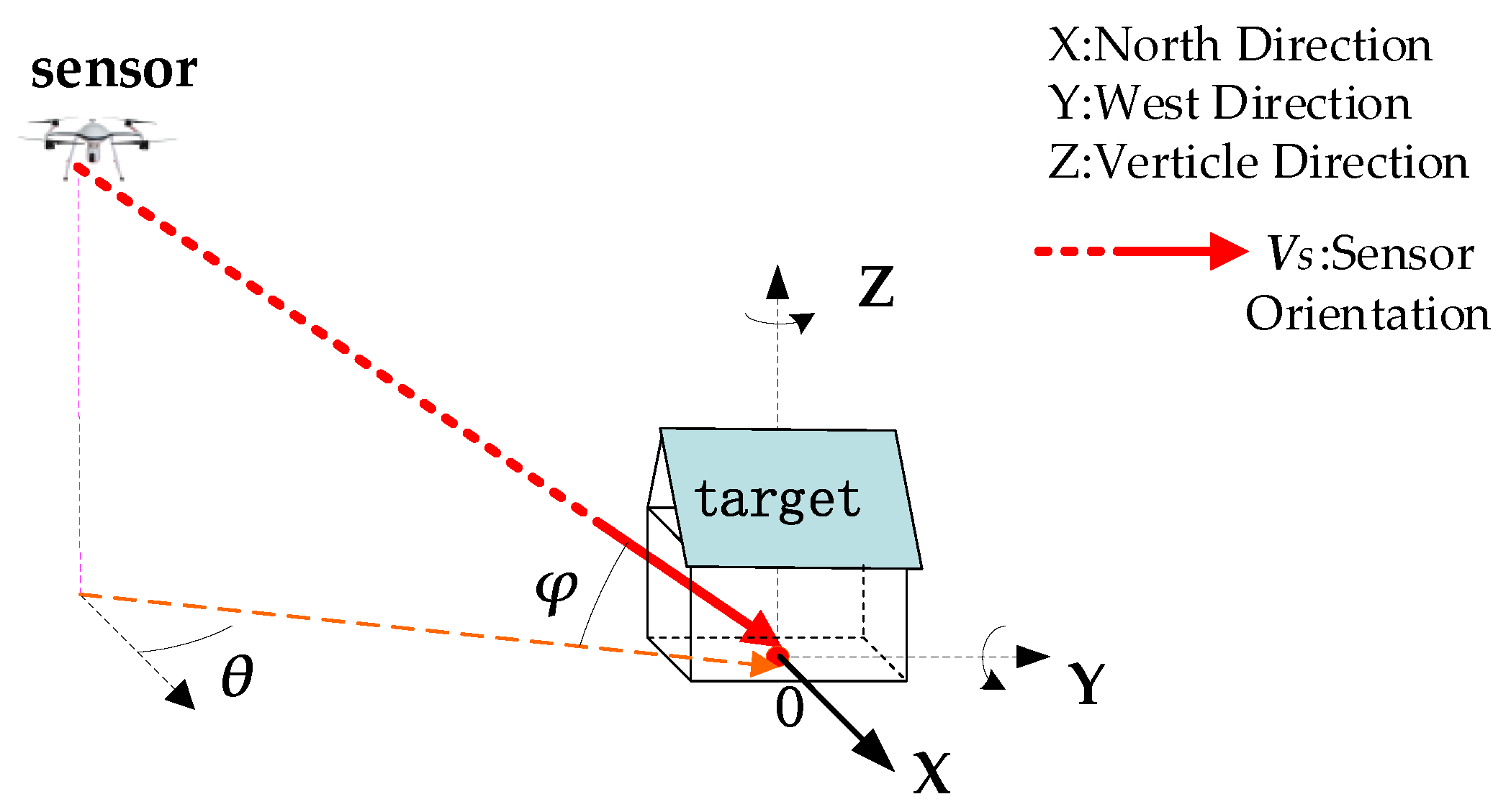
2.1. Definition of Drone Observation Angles

The definitions of UAV observation angles are as follows: establish a three-dimensional Cartesian coordinate system with the ground center of the target building as the coordinate origin, the north direction as the X-axis, the horizontal direction perpendicular to it as the Y-axis, and the vertical direction as the Z-axis. Assume that the observation direction vector of the UAV sensor is V_S, which points from the imaging center of the sensor to the ground center of the target all the time. The ground center position of the target can be determined by previous positioning and detection. Since the ground center position of the target is known, the position of each waypoint can be determined by RAA and RDA. The definition and schematic diagram of RAA and RDA are shown in Figure 1.

The relative azimuth angle θ is defined as the angle between the projection vector of V_S on the horizontal plane and the positive direction of the X-axis. The value range is [0, 90] with a unit of degrees (°). When viewed from the positive half-axis of the Z-axis to the XOY plane, the angle increases counterclockwise.

The relative depression angle φ is defined as the angle between V_S and its projection vector on the horizontal plane. The value range is [0, 90] with a unit of degree (°). When viewed from the positive Y-axis of the XOZ plane, the angle increases counterclockwise.

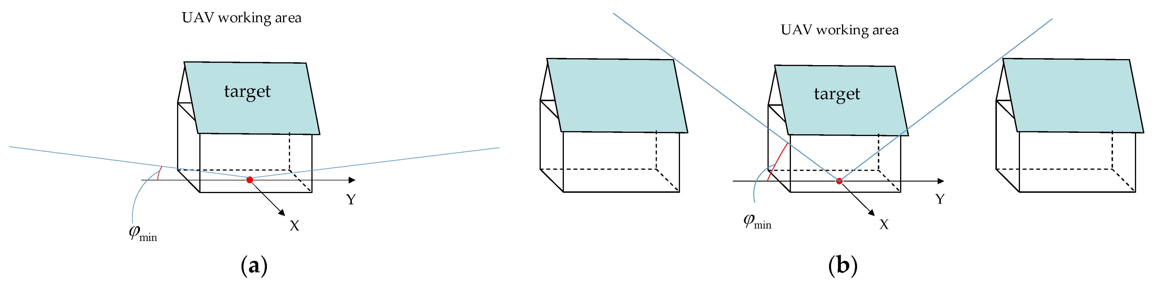
2.2. Analysis of Constraints for UAV Observations

2.2.1. Constraints on RDA

The RDA is a key parameter in the acquisition of information for target buildings. According to the definition in Section 2.1, an angle of 90° is a vertical observation. When considering the UAV’s RDA, environmental factors also need to be taken into account. The UAV’s RDA is considered in two cases. They are discussed below and the schematic diagram of each case is shown in Figure 2.

(a) When the surroundings of the target building are spacious without other tall buildings or obstructions, the UAV can perform multi-altitude circumnavigation flights around the target building. The range of values for RDA is:

$${\phi }_{\min }\le \phi \le {90}^{°}$$

(1)

For safety reasons, the UAV will not fly too close to the ground. To avoid collisions with obstacles such as trees on the ground, the minimum value of the RDA φ_min should be limited to a small value.

(b) When there are other tall buildings or facilities around the target building, the UAV cannot perform multi-altitude circumnavigation flights. The minimum flight height of the UAV should not be less than the height of the target building itself or the highest surrounding buildings. In this case, the range of values for the RDA is: ${\phi }_{\min }\le \phi \le {90}^{°}$.

2.2.2. Constraints on RAA

The constraints on RAA are usually caused by environmental factors. In case a, the UAV can fly around the target buildings without obstructions, and therefore the range of values for RAA is: 0° ≤ θ ≤ 360°. In the other case, the RDA is no less than 45°,which means that the UAV should fly above the highest building around. In other words, the range of values for RAA is still: 0° ≤ θ ≤ 360°.

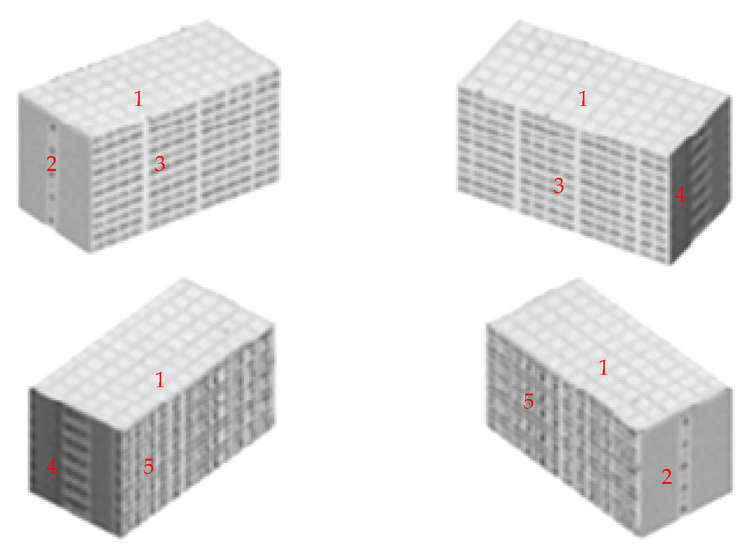
2.3. A Multi-Angle Target Information Acquisition Model

In order to reasonably evaluate the quality of the surface information, assume that the sensor observes the target A at the angle (θ, φ), which can be described by a vector G(θ, φ, T_S) composed of all N surfaces (m top surfaces, n side surfaces, N = n + m). G is shown in the following equation:

$$G(\theta ,\phi )=[I_{F_1}(\theta ,\phi ,T_{S\_1}),I_{F_2}(\theta ,\phi ,T_{S\_2}),\cdots ,I_{F_{N-1}}(\theta ,\phi ,T_{S\_N-1}),I_{F_N}(\theta ,\phi ,T_{S\_N})]$$

(2)

where $I_{F_i}\left(\theta ,\phi ,T_{S\_i}\right)$ (i = 1, 2,…, N) represents information acquired of the ith surface by the sensor. $I_{F_i}\left(\theta ,\phi ,T_{S\_i}\right)$ is considered as a function of the sensor’s RAA, RDA, and the orientation of the target face. Based on the analysis of the angle constraints factors in the previous text, the orientation of the target surface can be represented as (θ_{s_i}, φ_{s_i}), where θ_{s_i} ∈ [0°, 360°], φ_{s_i} ∈ [−90°, 0°]. The information acquisition situation of the current surface can be expressed as follows:

$$I_{F_i}(\theta ,\phi ,T_{S\_i})=\left\{\begin{array}{l}{I}_{F_i}(\theta -{\theta }_{S\_i},\phi -{\phi }_{S\_i}), \theta -{\theta }_{S\_i}\in (-{270}^{°},-{90}^{°})\cup ({90}^{°},{270}^{°})\\ 0, otherwise\end{array}\right.$$

(3)

The equation means that information can only be obtained when the sensor observes the target surface within a 180-degree range. Otherwise, no information can be obtained.

Considering the information acquisition of a single surface from different observation angles, a statistical model based on the image entropy ratio (IER) is proposed to evaluate the information quantity. The IER of a certain surface of the target is defined as follows:

$$IER(\alpha ,\beta )=\left|\frac{E(\alpha ,\beta )-E_{ort}}{E_{ort}}\right|=\left|\frac{-{\displaystyle \sum _{i=1}^k{P}_{\alpha \beta \_i}{\log }_2(P_{\alpha \beta \_i})}+{\displaystyle \sum _{i=1}^k{P}_{ort\_i}{\log }_2(P_{ort\_i})}}{-{\displaystyle \sum _{i=1}^k{P}_{ort\_i}{\log }_2(P_{ort\_i})}}\right|$$

(4)

where α and β respectively refer to the horizontal deviation angle and the vertical deviation angle between the observation direction and the observed surface. α = |θ − θ_s|, β = |φ − φ_s|. $E_{ort}$ represents the entropy of the frontal view of the observed surface, and $E(\alpha ,\beta )$ represents the entropy of the tilted view at the corresponding viewing angle. $P_{\alpha \beta \_i}$ and $P_{ort\_i}$ represent the distribution probabilities of each gray level in the two images. Obviously, IER is a dimensionless ratio that measures the difference between the information obtained at different viewing angles and the information of the frontal view image. The value range of IER is [0, 1]. The closer IER is to 0, the less information is lost. When IER = 1, there is no information acquired. Let IER(α,β) = 1 − $I_{F_i}\left(\theta ,\phi ,T_{S\_i}\right)$, which can be used to describe the information loss rate of the observed surface at the viewing angle (θ, φ). Due to the existence of occlusion, only when α is between 90° and 270°, IER(α, β) ≠ 1. The goal function is to find the minimum IER of all surfaces; therefore, all solutions that make IER = 1 are abandoned in the process of iteration. The trend of IER is that the observation angle is closer to the front view, the corresponding IER(α, β) value is smaller.

Furthermore, if a multi-angle observation method based on K points is used to observe the target, the information acquired of each observation point can be represented by a matrix P_K×N:

$$P=\left[\begin{array}{c}{G}_{R{S}_1}({\theta }_1,{\phi }_1,T_{S\_i})\\ G_{R{S}_2}({\theta }_2,{\phi }_2,T_{S\_i})\\ ⋮\\ G_{R{S}_{K-1}}({\theta }_{K-1},{\phi }_{K-1},T_{S\_i})\\ G_{R{S}_K}({\theta }_K,{\phi }_K,T_{S\_i})\end{array}\right]=\left[\begin{array}{c}{I}_{S_1}\left({\theta }_1,{\phi }_1,T_{S\_1}\right),I_{S_2}\left({\theta }_1,{\phi }_1,T_{S\_2}\right),\dots ,I_{S_{N-1}}\left({\theta }_1,{\phi }_1,T_{S\_N-1}\right),I_{S_N}\left({\theta }_1,{\phi }_1,T_{S\_N}\right)\\ I_{S_1}\left({\theta }_2,{\phi }_2,T_{S\_1}\right),I_{S_2}\left({\theta }_2,{\phi }_2,T_{S\_2}\right),\dots ,I_{S_{N-1}}\left({\theta }_2,{\phi }_2,T_{S\_N-1}\right),I_{S_N}\left({\theta }_2,{\phi }_2,T_{S\_N}\right)\\ ⋮\\ I_{S_1}\left({\theta }_{K-1},{\phi }_{K-1},T_{S\_1}\right),I_{S_2}\left({\theta }_{K-1},{\phi }_{K-1},T_{S\_2}\right),\dots ,I_{S_{N-1}}\left({\theta }_{K-1},{\phi }_{K-1},T_{S\_N-1}\right),I_{S_N}\left({\theta }_{K-1},{\phi }_{K-1},T_{S\_N}\right)\\ I_{S_1}\left({\theta }_K,{\phi }_K,T_{S\_1}\right),I_{S_2}\left({\theta }_K,{\phi }_K,T_{S\_2}\right),\dots ,I_{S_{N-1}}\left({\theta }_K,{\phi }_K,T_{S\_N-1}\right),I_{S_N}\left({\theta }_K,{\phi }_K,T_{S\_N}\right)\end{array}\right]$$

(5)

Normally, multiple points may simultaneously observe a certain surface, and the  $I_{F_i}\left(\theta ,\phi ,T_{S\_i}\right)$ quality of each observation point corresponding to that surface may not be the same. Therefore, the minimum IER is selected to evaluate the information loss. The information loss $\Delta$ of the target observed by the K observation point method is:

$$\Delta ={\displaystyle \sum \min IER(\alpha ,\beta )}={\displaystyle \sum _{i=1}^N\min [1-I_{F_i}(\theta -{\theta }_{S\_i},\phi -{\phi }_{S\_i})}]$$

(6)

which is the Adequacy Evaluation Model for Multi-angle-based Stereo Information Acquisition (AE-MSIA model).

To obtain IER, a UAV remote sensing observation target simulation system is built. Firstly, images of the simulation target at different angles are obtained. The resolution of the simulation image is 0.5 m/pixel. In the simulation system, RAA θ is sampled every 3° within 1°~360° (124 angles), and RDA φ is sampled every 3° within 0°~90° (30 angles). The images at 3720 angles are obtained. The IER values of the corresponding angles are calculated, and then we use polynomial curve fitting to acquire the relationship between IER and RAA and RDA. The mean square error of fitting is 0.01. Figure 3 gives examples of simulated images at four different viewing angles. As the figure shows, there are five surfaces of a target. At different viewing angles, the surfaces that can be seen are different, and the IER obtained is different.

3. Proposed Method

3.1. Artificial Bee Colony Algorithm

The ABC algorithm is an algorithm that simulates the foraging behavior of bees, which was proposed by Dervis Karaboga et al. in 2005 [32]. When performing the foraging task, bee colonies are divided into three roles: employed bee, onlooker bee, and scout bee (abbreviated as E-bee, O-bee, and S-bee). E-bees are mainly responsible for global optimization; O-bees are mainly responsible for fine-grained local search in the neighborhood of the various solutions found by E-bees; and S-bees are used for initialization and to generate new solutions to prevent the algorithm from getting stuck in local optima after an individual has not been updated for multiple iterations. While the bee colony seeks to obtain the maximum amount of nectar, the ABC algorithm searches for the variable vector corresponding to the minimum value of the objective function.

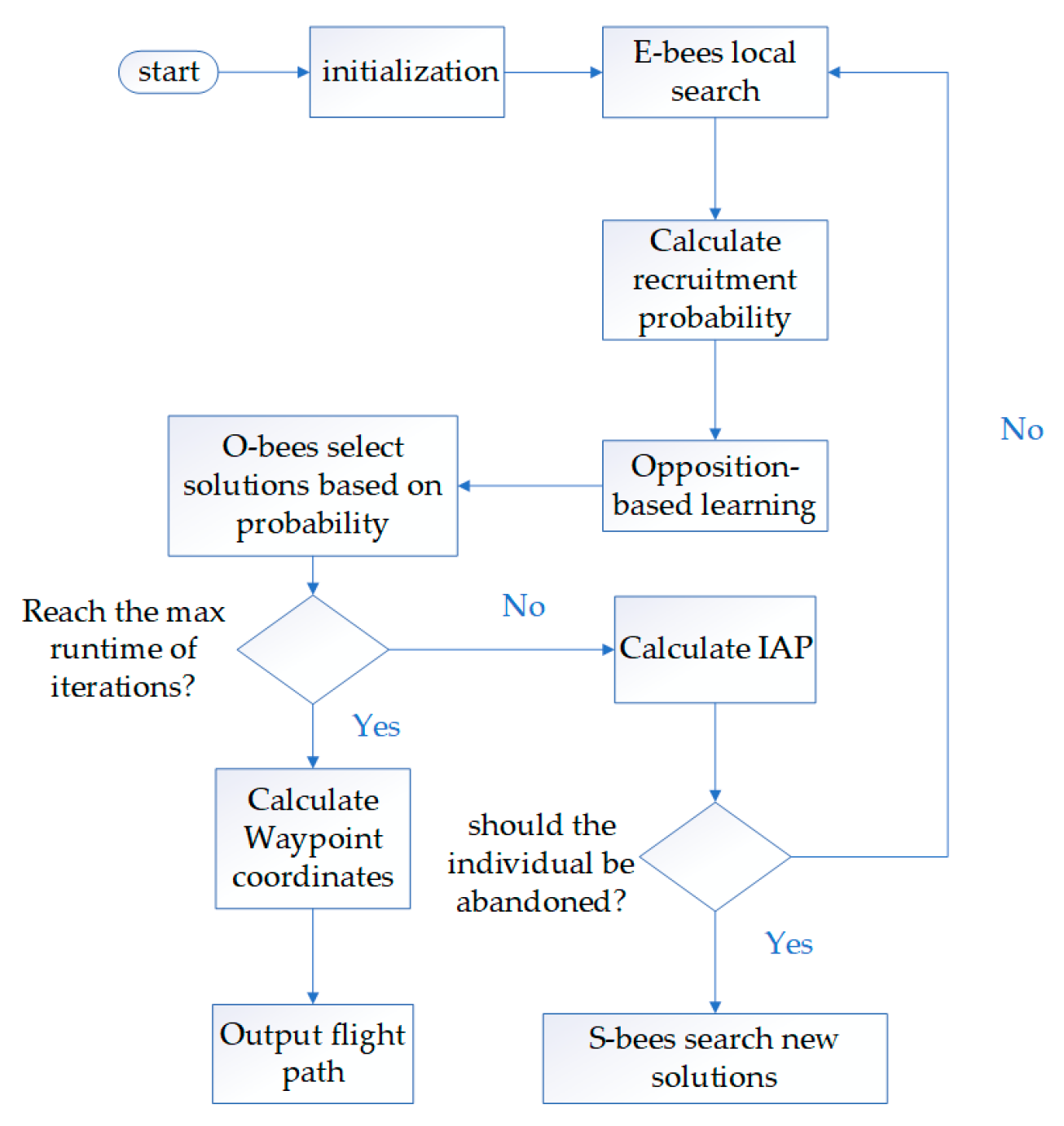
3.2. Opposition-Based Learning Artificial Bee Colony Algorithm

The ABC algorithm excels due to its simple parameter settings and fast convergence speed. However, it is still easy for the algorithm to fall into local optimal solutions. In order to solve this problem, this paper proposes an improved ABC algorithm utilizing an opposition-based learning mechanism.

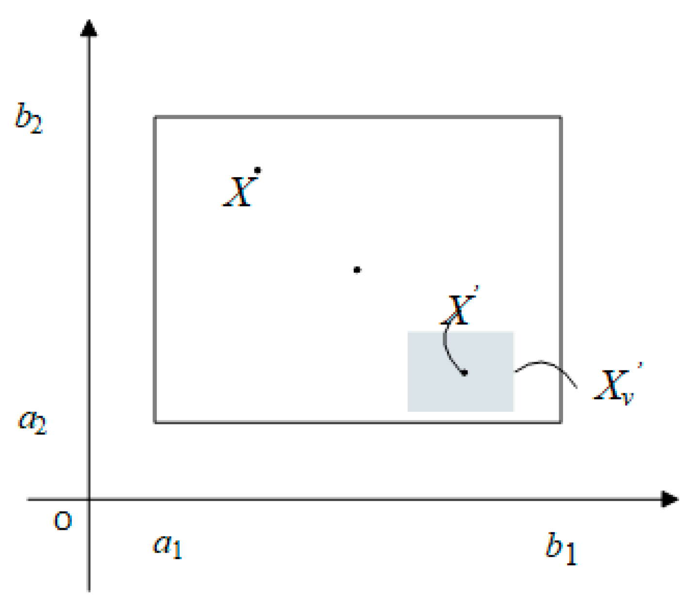
3.2.1. Opposition-Based Learning Mechanism

Rahnamayan and colleagues [33] first proposed the concept of opposition-based learning; here are some of the basic concepts:

For a given $x\in [a,b]$, its bit point $x^{\prime }$ is defined as:

$$x^{\prime }=a+b-x$$

(7)

Similarly, there are bit points for points in multidimensional spaces as well:

Assume $X=(x_1,x_2,\cdots ,x_D)$ is a point in a D-dimensional space, where $x_i\in [a_i,b_i]$; then, for the bit point $X^{\prime }=(x_1^{\prime },x_2^{\prime },\cdots ,x_D^{\prime })$, its components are $x_i^{\prime }=a_i+b_i-x_i$.

Assume $X=(x_1,x_2,\cdots ,x_D)$ is a point in a D-dimensional space, where $x_i\in [a_i,b_i]$; then, for the vague bit point $X_v^{\prime }=(x_{v1}^{\prime },x_{v2}^{\prime },\cdots ,x_{vD}^{\prime })$, its components are $x_{vi}^{\prime }=\mathrm{rand}(0,1)(a_i+b_i)-x_i$.

As Figure 4 shows, the traditional opposition-based learning mechanism generates bit point $X^{\prime }$, which can be seen as a point symmetrical about the geometric center of the space in a multidimensional space. Instead of a certain location, vague opposition-based learning introduces randomness. The new vague bit point is generated within a random range (the shaded part of Figure 4). The advantage of the new mechanism is expanding the selection range in the multidimensional space.

Introducing vague bit points to the ABC algorithm optimizes the E-bees’ search for new solutions. In the traditional ABC algorithm, after completing the current iteration, the offspring bees conduct a local search to generate new solutions. After introducing the opposition-based learning mechanism, the algorithm evaluates the quality of all individuals in the current population—which means all solutions found in the current search—in terms of their profits. It selects SN/2 individuals with lower profits to perform vague bit point operations and calculates their profits. The algorithm selects the next generation with higher quality. The introduction of bit points improves the quality of the initial solutions in the next generation, and only half of the population with lower profits undergoes bit point operations. This retains the algorithm’s complexity with higher-quality solutions, without requiring more resources. The opposition-based learning generally used to generate bit points is:

$$x_{vij}^{\prime }={\min }_j+{\max }_j-x_{vij}+\mathrm{rand}(-R,R)({\min }_j+{\max }_j)$$

(8)

where $x_{ij}$ represents the jth dimension of the ith individual in the population, and ${\min }_j$ and ${\max }_j$ represent the minimum and maximum values of the search range for the jth dimension. R is a parameter used to control the range of vague opposition-based learning. To keep the individual within the search area as much as possible, R = 0.125.

3.2.2. Improved S-Bee Search Mechanism

During the S-bee search phase, it is meant to discard a solution after it has remained unchanged for a predetermined constant limited number of consecutive generations. This is to enhance the algorithm’s global search capabilities to ensure that the algorithm does not prematurely converge to a local optimum. However, setting the limit as a constant can lead to many drawbacks:

(1) It is difficult to find a unified standard for the parameter limit for different optimization problems. An improper setting of the limit may affect the algorithm’s global search capabilities.

(2) Discarding solutions directly may also discard some high-quality solutions.

Therefore, it is unreasonable to only consider the number of times a solution has not been updated without considering its fitness value. Based on these reasons, the following improved method is used for the search and judgment of the S-bee:

For a population of N individuals, each individual is represented by a D-dimensional vector: $x_{ij}=\left\{x_{i1},x_{i2},\cdots \cdots , x_{ij},\cdots \cdots x_{iD}\right\}$, $j=1,2,\cdots \cdots ,D$, $i=1,2,\cdots \cdots ,N$.

In order to measure population diversity, the center of the jth dimension of the solutions is defined as:

$${\overline{x}}_j=\frac{1}{N}{\displaystyle \sum _{i=1}^N{x}_{ij}}$$

(9)

The individual abandonment criterion is defined as follows:

$$E\mathrm{s}{p}_i=\frac{tria{l}_i}{di{s}_i}$$

(10)

where $tria{l}_i$ represents the number of unchanged times of individual $X_i$, and $di{s}_i$ represents the impact of the individual on population diversity, and is calculated by the following equation:

$$di{s}_i=\frac{1}{D}{\displaystyle \sum _{j=1}^D\Vert x_{ij}-\overline{x_j}\Vert }$$

(11)

As the equation shows, $di{s}_i$ measures the individual’s impact on population diversity.

The larger $di{s}_i$ is, the larger the distance that the individual is from the center of the population, and the more unique the individual is. On the other hand, $E\mathrm{s}{p}_i$ takes both the number of times a solution has not been updated and the individual’s impact on population diversity into account. A larger $E\mathrm{s}{p}_i$ means a higher probability that the individual will be discarded.

The individual abandonment probability (IAP) is defined as follows:

$$P_{\mathrm{i}}=\frac{Es{p}_i-\mathrm{Min}(Es{p}_i)}{\mathrm{Max}(Es{p}_i)-\mathrm{Min}(Es{p}_i)}$$

(12)

When abandoning solutions, a comparison is made between $P_{\mathrm{i}}$ and rand (0, 1). If $P_{\mathrm{i}}$ is greater, it means that the solution should be abandoned and the S-bees will search for a new solution. Through the individual abandonment probability, individuals that contribute highly to the diversity of the population are preserved, enhancing the population diversity. With it, individuals do not gather in large numbers on some particular locations. In other words, it can prevent a large number of waypoints from observing the target from similar angles. This also makes the activation mechanism of the scout bees adaptive.

The process of OABC is shown in Figure 5.

4. Experiment

4.1. Controlled Experiment

4.1.1. Experiment Design

Given the significant difference in the range of RDAs in the presence and absence of obstructions around the target buildings, the controlled experiment was divided into two scenes for discussion.

Scene 1: There are obstructions around the target building.

The RDA range for flight is: ${30}^{°}\le \phi \le {90}^{°}$

Scene 2: There are no obstructions around the target building.

The RDA range for flight is: $5^{°}\le \phi \le {90}^{°}$

To demonstrate the superior performance of the OABC algorithm, it was compared with the ABC algorithm, ant colony optimization (ACO) algorithm, evolutionary algorithm (EA), and two enhanced ABC algorithms. The first one is from reference [28], abbreviated as ABC1, and the second one is from reference [34], abbreviated as ABC2. These two algorithms are relatively new and have been proven to have good performance. The algorithms were tested in two scenes with the same population size, run for 1000 iterations each, and repeated 50 times. The mean, standard deviation, and average runtime of iteration results were calculated for each algorithm.

4.1.2. Experiment Results

Scene 1: There are obstructions around the target building.

In a certain iteration, 25 waypoints were generated, and the route set by them is shown in the following Figure 6. The statistical results of 50 experiments are shown in

Table 1. Comparison of algorithms performance as the population size varied in Scene 1.

Population Size	Algorithm	Mean	Std	Time (s)
10	EA	3.6854	0.1352	56.17
	ACO	1.9787	0.0368	53.18
	ABC	1.5870	0.0358	51.33
	ABC1	1.3406	0.0271	53.01
	ABC2	1.2696	0.0289	48.62
	OABC	1.2313	0.0154	46.98
20	EA	3.425	0.1277	87.59
	ACO	1.8390	0.0423	71.63
	ABC	1.4135	0.0312	73.88
	ABC1	1.3048	0.0229	73.94
	ABC2	1.2501	0.0247	79.16
	OABC	1.2309	0.0124	66.51
30	EA	3.1183	0.1049	123.88
	ACO	1.7581	0.0364	121.68
	ABC	1.3537	0.0291	127.80
	ABC1	1.2425	0.0119	126.36
	ABC2	1.2310	0.0202	124.97
	OABC	1.2309	0.0103	104.32
50	EA	2.8609	0.1124	348.98
	ACO	1.6872	0.0387	215.08
	ABC	1.3431	0.0272	226.95
	ABC1	1.2356	0.0119	209.64
	ABC2	1.2309	0.0182	199.02
	OABC	1.2310	0.0112	175.94
100	EA	2.5439	0.0847	580.61
	ACO	1.4598	0.0301	422.50
	ABC	1.2315	0.0243	450.13
	ABC1	1.2310	0.0089	426.98
	ABC2	1.2309	0.0104	412.52
	OABC	1.2308	0.0092	384.39

Bold numbers represent the best result in the corresponding section. So are the rest of the tables.

.

As can be seen from Figure 7, when the population size was small (less than 20), the OABC algorithm outperformed the other algorithms. The mean and standard deviation of OABC were lower than any other algorithm. The mean of ABC2 was very close to that of OABC, which was only 0.7% higher. However, the standard deviation of ABC2 was 40% larger than that of OABC. It is demonstrated that OABC algorithm can converge to the optimal solution stably with less sources. When the population size was large, the performances of OABC, ABC1, and ABC2 were very similar. However, OABC algorithm took 7% less time than ABC2 and 11% less time than ABC1. In conclusion, the OABC algorithm is able to converge to the optimal solution more quickly and stably than the other algorithms.

Scene 2: There are no obstructions around the target building.

In a certain iteration, 23 waypoints were generated, and their distribution is shown in Figure 8. The statistical results of 50 experiments are shown in

Table 2. Comparison of different algorithms as the population size varied in Scene 2.

Population Size	Algorithm	Mean	Std	Time (s)
10	EA	2.1192	0.1488	59.64
	ACO	0.9463	0.0618	53.49
	ABC	0.7732	0.0472	52.97
	ABC1	0.7763	0.0366	49.32
	ABC2	0.6289	0.0291	47.40
	OABC	0.6051	0.0209	47.96
20	EA	1.8970	0.1358	89.84
	ACO	0.9234	0.0589	81.06
	ABC	0.7156	0.0433	82.58
	ABC1	0.6949	0.0315	77.20
	ABC2	0.6593	0.0256	75.98
	OABC	0.6050	0.0182	73.44
30	EA	1.2312	0.1586	178.48
	ACO	0.8865	0.0378	137.29
	ABC	0.6954	0.0395	142.65
	ABC1	0.6617	0.0292	126.89
	ABC2	0.6201	0.0226	102.76
	OABC	0.6049	0.0136	102.88
50	EA	0.9873	0.0973	354.36
	ACO	0.7839	0.0423	229.10
	ABC	0.6723	0.0250	262.16
	ABC1	0.6130	0.0217	218.22
	ABC2	0.6050	0.0127	194.61
	OABC	0.6049	0.0129	173.20
100	EA	0.9857	0.0925	572.65
	ACO	0.6982	0.0247	461.60
	ABC	0.6154	0.0187	484.73
	ABC1	0.6050	0.0151	462.53
	ABC2	0.6049	0.0130	377.52
	OABC	0.6048	0.0127	343.85

.

The situation in Scene 2 has many similarities to Scene 1. When the population size was small, the mean and standard deviation of OABC were lower than any other algorithm, which is indicated in Figure 9a,b. As Figure 9c shows, although OABC and ABC2 consumed almost the same amount of time, the mean of ABC2 was 9.8% higher than that of OABC, and the standard deviation was 40.6% higher. When the population size was large, all enhanced ABC algorithms could converge to the optimal solution, but OABC was still 10% faster than the fastest algorithm of the others. In conclusion, in both Scene 1 and Scene 2, the OABC algorithm was able to converge to the optimal solution more quickly and stably than the other algorithms.

4.2. 3D Reconstruction Experiment

4.2.1. Experiment Design

To demonstrate that the OABC algorithm obtains more comprehensive building target information for path planning, 3D reconstruction was carried out on images obtained from actual buildings and the results were compared. We compared the performances of OABC, ABC, ABC1, ABC2, and five-direction flight. The five-direction flight is a built-in algorithm that is commonly used for oblique photography. The drone observes the target from five directions: front, back, left, right, and orthophoto photography of the building. A schematic diagram of five-direction flight is shown in Figure 10. Referring to reference [35], we set the parameters of five-direction flight. The forward overlap was 90%, the side overlap was 85%, and the oblique photogrammetry relative altitude was 140 m. The distance from the side of the building to the UAV camera was about 50 m according to the actual flight conditions.

During field work, it was found that the majority of buildings belonged to Scene 1, which means there are other high obstructions around them, so only Scene 1 was compared. It is worth mentioning that in order to meet the requirement of overlap for 3D reconstruction, all waypoints of the OABC and ABC algorithms were checked after being generated. If the requirement was not met, new waypoints were inserted equidistantly between adjacent waypoints until the overlap requirement was satisfied.

Drone platform: DJI M300 RTK

Sensor: Zenmuse P1

3D reconstruction platform: Context Capture

4.2.2. Visual Comparison of Models

Table 3. Comparison of 3D reconstruction models captured by different algorithms.

	Surface 1	Surface 2	Surface 3	Surface 4
OABC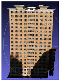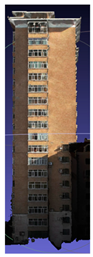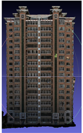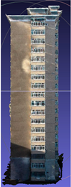
ABC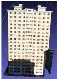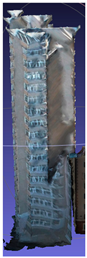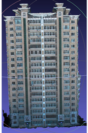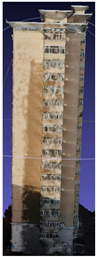
ABC1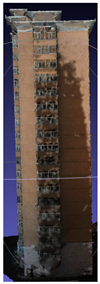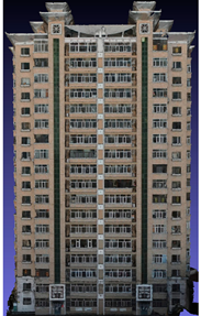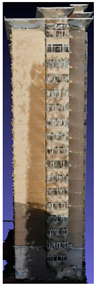
ABC2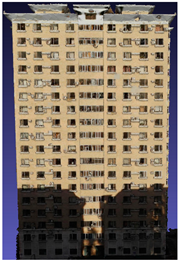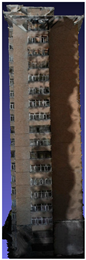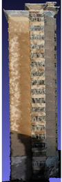
Five-directional flight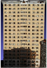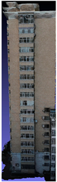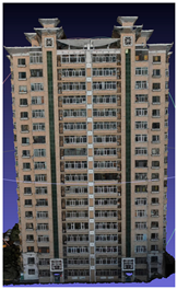

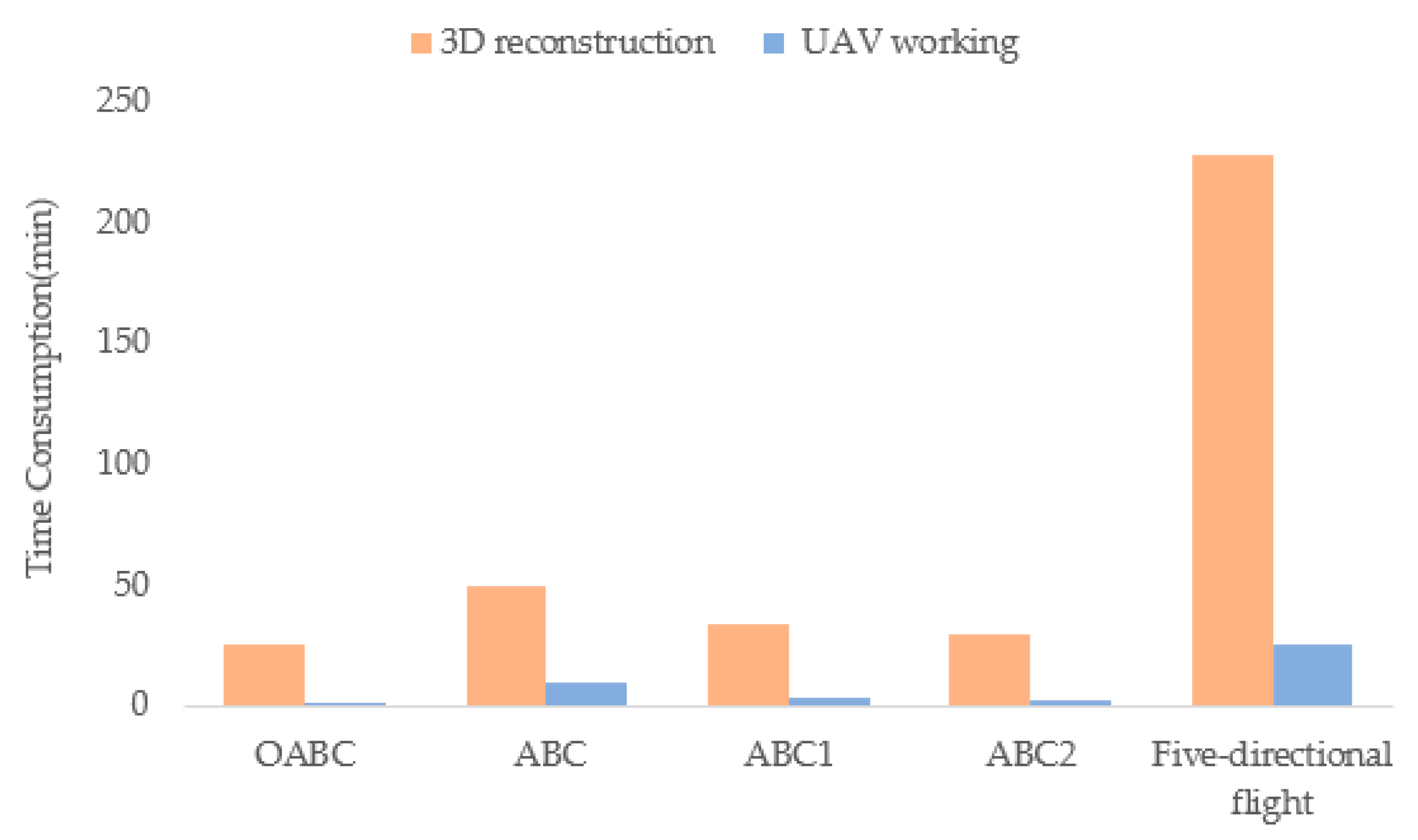
shows that all data acquisition methods reconstructed the target’s 3D model with complete models and basically correct spatial topology relationships between objects. The building’s important elements, such as roofs and eaves, are complete, which have some degree of detailed representation. Meanwhile, the comparison shows that the 3D model captured by five-direction flight has the best performance, with the fewest surface irregularities and protrusions. It is followed by the 3D model captured by the OABC algorithm. It has a few burrs and protrusions, which is slightly inferior to that of five-direction flight. The models captured by ABC1 and ABC2 have some distortions at the edges of the building, especially on the top of surface 2. The model from ABC2 has more serious distortions than that of ABC1. The model from ABC performs the worst, and its surface 2 is almost completely distorted. In conclusion, the order of visual comparison from best to worst is: five-directional flight, OABC, ABC1, ABC2, ABC. Additionally, the UAV working efficiency and 3D reconstruction efficiency of different algorithms are shown in

Table 4. Number of images and time consumption of UAV working and 3D reconstruction.

	Number of Images	Time Consumption of UAV Working	Time Consumption of 3D Reconstruction
OABC	25	2 min 10 s	25 min 46 s
ABC	52	10 min 13 s	50 min 20 s
ABC1	30	3 min 21 s	34 min 02 s
ABC2	28	2 min 43 s	30 min 27 s
Five-Directional Flight	89	25 min 46 s	3 h 48 min

. It is indicated that although the performance of five-direction flight surpassed the others, it took much more time. OABC had similar performance and took the least time for both drone operations and 3D reconstruction. That is the result of the visual comparison; quantitative comparison is as follows.

4.2.3. Quantitative Comparison

To further evaluate the accuracy of the algorithms for 3D building reconstruction, the geometric accuracy of the 3D models is compared below. The geometric accuracy of the model includes two measurements: planar accuracy and height accuracy. Planar accuracy can be obtained by calculating the root mean square error (RMSE) in the X direction and Y direction. Height accuracy is obtained by calculating the RMSE in the Z direction. The calculation method for RMSE is to capture the coordinates of ground feature points as the true values, and then measure the coordinates of the corresponding check points on the model. Finally, the RMSE is calculated [35,36,37].

In total, 30 points were measured on the target building for each algorithm, including but not limited to the corners and protrusions of the building’s roof. The results of geometric accuracy are shown in

Table 5. Geometric accuracy of all models.

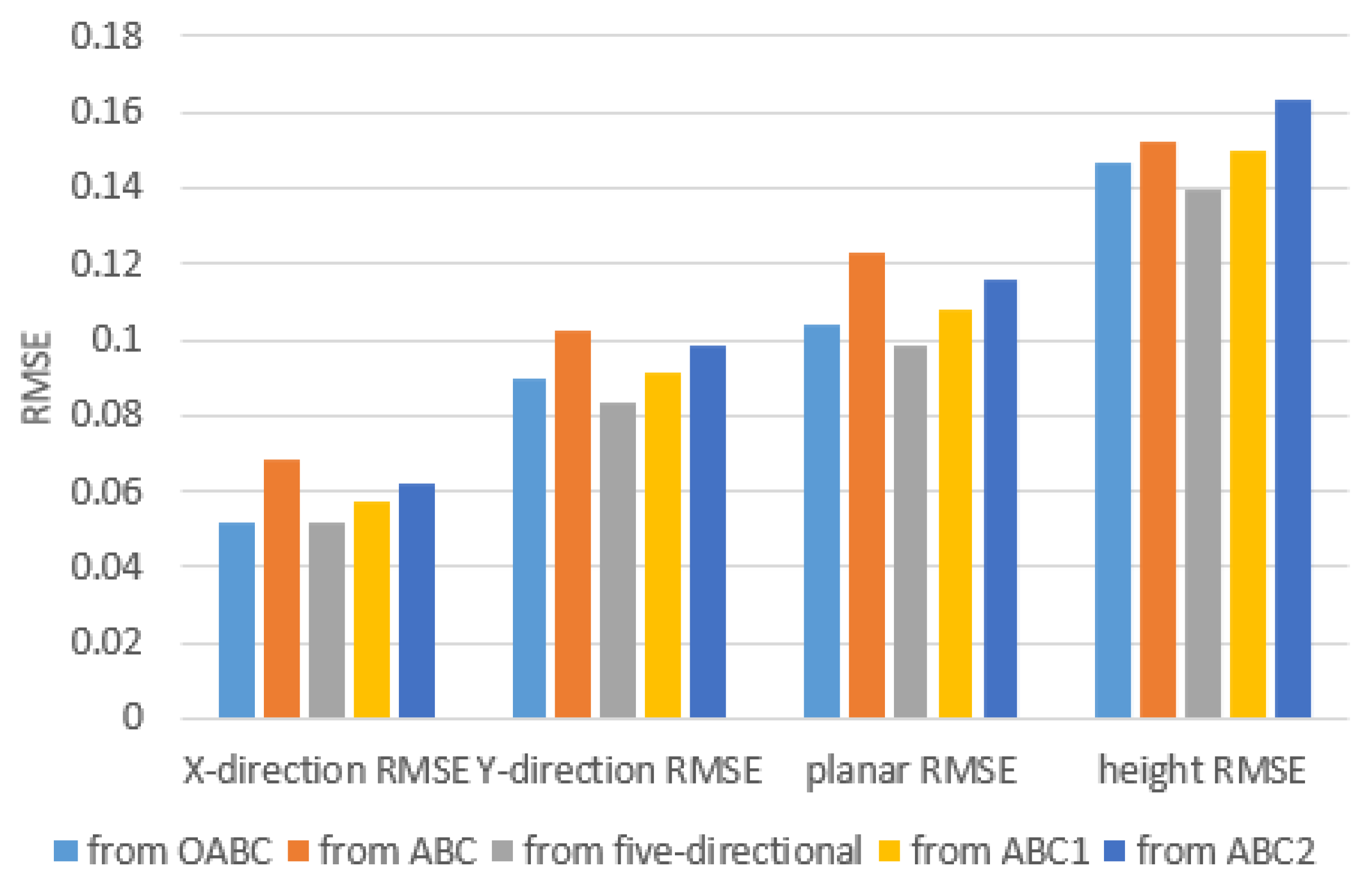
3D Models	X-Direction RMSE	Y-Direction RMSE	Planar RMSE	Height RMSE
From OABC	0.0515	0.0898	0.1036	0.1470
From ABC	0.0683	0.1023	0.1230	0.1522
From ABC1	0.0576	0.0917	0.1083	0.1497
From ABC2	0.0618	0.0984	0.1162	0.1633
From Five-Directional Flight	0.0521	0.0835	0.0984	0.1395

.

Figure 11 shows that the 3D reconstruction results from images captured by the OABC method are better than those captured by ABC1 and ABC2, with a reduction of at least 4.5% in the planar RMSE and at least 2% in the height RMSE. Figure 12 shows that although the planar and height RMSE were slightly higher than those captured by the five-directional flight, which are about 5% higher, the drone work efficiency and 3D reconstruction efficiency were greatly improved. This proves that the OABC algorithm optimizes UAV path planning by obtaining basically the same amount of information in a much shorter time.

5. Conclusions

This paper proposes an opposition-based learning ABC algorithm for UAV information acquisition. By introducing an opposition-based learning mechanism, the E-bees can search a wider area in a single iteration, which enhances the global search capability and increases the convergence speed. Moreover, the S-bees activation mechanism is improved by proposing a new mechanism that can adaptively adjust the individual abandon probability based on both the number of times an individual has not been updated and the relative position of the population. The diversity of the population and the robustness of the algorithm are enhanced. In Section 4, the proposed OABC algorithm is compared with other path planning algorithms. The experiment results show that when the population size is small (≤20), while the OABC algorithm can converge to the optimal solution, other algorithms cannot. The mean of OABC is lower than any other algorithm, and the standard deviation is at least 40% lower, proving that the algorithm is more stable and can escape from local optima. When the population size is large (100), other enhanced ABC algorithms can converge to the optimal solution too, but they take 7% more time. This proves that the OABC algorithm can find the optima more quickly and stably with fewer resources.

To verify the performance of the algorithm, actual target building images were obtained through UAV for 3D reconstruction. The proposed method was compared with other methods in terms of the accuracy of the 3D models, the time required, and the UAV operation time. The results show that the proposed method can greatly improve the efficiency of UAV operations and accelerate the speed of 3D reconstruction while ensuring the accuracy of 3D reconstruction. The planar error of the proposed method is 4.5% smaller than those of the other ABC algorithms, and the height error is 2% smaller. Although the error is increased by about 5% compared with the five-directional flight algorithm, UAV operation time and 3D reconstruction time are significantly reduced. This proves that the proposed method can obtain more information in less time, which is of great contribution for subsequent processing.

In the end, we would like to discuss a problem affecting the application of drones: they lack suitable security mechanisms that protect them from various attacks. A drone’s flight controller and ground control station both have security vulnerabilities that could lead to cyber or physical attacks [38]. Reference [39] shows that a vulnerability has been discovered in the DJI UAVs that an attacker is able to exploit to gain user account information, which then leads to UAV hijacking. Considering that UAVs are increasingly used in urban situations, it is a growing challenge for UAV manufacturers and researchers to improve the security of UAV communication.

References

- Jin, P.; Mou, L.; Xia, G.-S.; Zhu, X.X. Anomaly Detection in Aerial Videos with Transformers. IEEE Trans. Geosci. Remote Sens. 2022, 60, 5628213. [Google Scholar] [CrossRef]
- Triantafyllia-Maria, P.; Antonios, M.; Dimitrios, T.; Georgios, M. Water Surface Level Monitoring of the Axios River Wetlands, Greece, Using Airborne and Space-Borne Earth Observation Data. In Proceedings of the IGARSS 2022–2022 IEEE International Geoscience and Remote Sensing Symposium, Kuala Lumpur, Malaysia, 17–22 July 2022; IEEE: Toulouse, France, 2022; pp. 6205–6208. [Google Scholar]
- Jhan, J.-P.; Kerle, N.; Rau, J.-Y. Integrating UAV and ground panoramic images for point cloud analysis of damaged building. IEEE Geosci. Remote Sens. Lett. 2021, 19, 6500805. [Google Scholar] [CrossRef]
- Zhan, P.; Song, C.; Luo, S.; Liu, K.; Ke, L.; Chen, T. Lake level reconstructed from DEM-based virtual station: Comparison of multisource DEMs with laser altimetry and UAV-LiDAR measurements. IEEE Geosci. Remote Sens. Lett. 2021, 19, 6502005. [Google Scholar] [CrossRef]
- Chen, H.; Li, Y. Dynamic view planning by effective particles for three-dimensional tracking. IEEE Trans. Syst. Man Cybern. (Cybern.) 2008, 39, 242–253. [Google Scholar] [CrossRef]
- Xia, Z.; Du, J.; Wang, J.; Jiang, C.; Ren, Y.; Li, G.; Han, Z. Multi-agent reinforcement learning aided intelligent UAV swarm for target tracking. IEEE Trans. Veh. Technol. 2021, 71, 931–945. [Google Scholar] [CrossRef]
- Yao, A.; Huang, M.; Qi, J.; Zhong, P. Attention mask-based network with simple color annotation for UAV vehicle re-identification. IEEE Geosci. Remote Sens. Lett. 2021, 19, 8014705. [Google Scholar] [CrossRef]
- Chang, J.; Dong, N.; Li, D.; Ip, W.H.; Yung, K.L. Skeleton Extraction and Greedy-Algorithm-Based Path Planning and its Application in UAV Trajectory Tracking. IEEE Trans. Aerosp. Electron. Syst. 2022, 58, 4953–4964. [Google Scholar] [CrossRef]
- Ding, Y.; Xin, B.; Dou, L.; Chen, J.; Chen, B.M. A memetic algorithm for curvature-constrained path planning of messenger UAV in air-ground coordination. IEEE Trans. Autom. Sci. Eng. 2021, 19, 3735–3749. [Google Scholar] [CrossRef]
- Yu, Z.; Sun, F.; Lu, X.; Song, Y. Overview of research on 3d path planning methods for rotor uav. In Proceedings of the 2021 International Conference on Electronics, Circuits and Information Engineering (ECIE), Zhengzhou, China, 22–24 January 2021; IEEE: Toulouse, France, 2021; pp. 368–371. [Google Scholar]
- Liu, H. A Novel Path Planning Method for Aerial UAV based on Improved Genetic Algorithm. In Proceedings of the 2023 Third International Conference on Artificial Intelligence and Smart Energy (ICAIS), Coimbatore, India, 2–4 February 2023; IEEE: Toulouse, France, 2023; pp. 1126–1130. [Google Scholar]
- Zhu, Z.; Qian, Y.; Zhang, W. Research on UAV Searching Path Planning Based on Improved Ant Colony Optimization Algorithm. In Proceedings of the 2021 IEEE 3rd International Conference on Civil Aviation Safety and Information Technology (ICCASIT), Changsha, China, 20–22 October 2021; IEEE: Toulouse, France, 2021; pp. 1319–1323. [Google Scholar]
- Luo, Q.; Wang, H.; Zheng, Y.; He, J. Research on path planning of mobile robot based on improved ant colony algorithm. Neural Comput. Appl. 2020, 32, 1555–1566. [Google Scholar] [CrossRef]
- Zhao, H.; Zhao, J. Improved ant colony algorithm for path planning of fixed wing unmanned aerial vehicle. In Proceedings of the 2021 International Conference on Physics, Computing and Mathematical (ICPCM2021), MATEC Web of Conferences, Xiamen, China, 29–30 December 2021; EDP Sciences: Les Ulis, France, 2022; p. 03002. [Google Scholar]
- Bao, S.; Lu, Y.; Li, K.; Xu, P. Research on path planning of UAV based on ant colony algorithm with angle factor. J. Phys. Conf. Ser. 2020, 1627, 012008. [Google Scholar] [CrossRef]
- Shao, S.; Peng, Y.; He, C.; Du, Y. Efficient path planning for UAV formation via comprehensively improved particle swarm optimization. ISA Trans. 2020, 97, 415–430. [Google Scholar] [CrossRef]
- Panda, M.; Das, B.; Pati, B.B. Grey wolf optimization for global path planning of autonomous underwater vehicle. In Proceedings of the Proceedings of the Third International Conference on Advanced Informatics for Computing Research, Shimla, India, 15–16 June 2019; ACM: New York, NY, USA, 2019; pp. 1–6. [Google Scholar]
- Mishra, M.; An, W.; Sidoti, D.; Han, X.; Ayala, D.F.M.; Hansen, J.A.; Pattipati, K.R.; Kleinman, D.L. Context-aware decision support for anti-submarine warfare mission planning within a dynamic environment. IEEE Trans. Syst. Man Cybern. Syst. 2017, 50, 318–335. [Google Scholar] [CrossRef]
- Hong, K.R.; O, S.I.; Kim, R.H.; Kim, T.S.; Kim, J.S. Minimum dose path planning for facility inspection based on the discrete Rao-combined ABC algorithm in radioactive environments with obstacles. Nucl. Sci. Tech. 2023, 34, 50. [Google Scholar] [CrossRef]
- Tan, L.; Shi, J.; Gao, J.; Wang, H.; Zhang, H.; Zhang, Y. Multi-UAV path planning based on IB-ABC with restricted planned arrival sequence. Robotica 2023, 41, 1244–1257. [Google Scholar] [CrossRef]
- Han, Z.; Chen, M.; Zhu, H.; Wu, Q. Ground threat prediction-based path planning of unmanned autonomous helicopter using hybrid enhanced artificial bee colony algorithm. Def. Technol. 2023. [Google Scholar] [CrossRef]
- Saeed, R.A.; Omri, M.; Abdel-Khalek, S.; Ali, E.S.; Alotaibi, M.F. Optimal path planning for drones based on swarm intelligence algorithm. Neural Comput. Appl. 2022, 34, 10133–10155. [Google Scholar] [CrossRef]
- Shen, L.; Hou, Y.; Yang, Q.; Lv, M.; Dong, J.-X.; Yang, Z.; Li, D. Synergistic path planning for ship-deployed multiple UAVs to monitor vessel pollution in ports. Transp. Res. Transp. Environ. 2022, 110, 103415. [Google Scholar] [CrossRef]
- Li, B.; Gong, L.-G.; Yang, W.-L. An improved artificial bee colony algorithm based on balance-evolution strategy for unmanned combat aerial vehicle path planning. Sci. World J. 2014, 2014, 232704. [Google Scholar] [CrossRef]
- Li, G.; Niu, P.; Xiao, X. Development and investigation of efficient artificial bee colony algorithm for numerical function optimization. Appl. Soft Comput. 2012, 12, 320–332. [Google Scholar] [CrossRef]
- Lu, C.; Lv, Y.; Su, Y.; Liu, L. UAV Swarm Collaborative Path Planning Based on RB-ABC. In Proceedings of the 2022 9th International Forum on Electrical Engineering and Automation (IFEEA), Zhuhai, China, 4–6 November 2022; IEEE: Toulouse, France, 2022; pp. 627–632. [Google Scholar]
- Zhu, G.; Kwong, S. Gbest-guided artificial bee colony algorithm for numerical function optimization. Appl. Math. Comput. 2010, 217, 3166–3173. [Google Scholar] [CrossRef]
- Peng, H.; Deng, C.; Wu, Z. Best neighbor-guided artificial bee colony algorithm for continuous optimization problems. Soft Comput. 2019, 23, 8723–8740. [Google Scholar] [CrossRef]
- Guo, P.; Cheng, W.; Liang, J. Global artificial bee colony search algorithm for numerical function optimization. In Proceedings of the 2011 Seventh International Conference on Natural Computation, Shanghai, China, 26–28 July 2011; IEEE: Toulouse, France, 2011; pp. 1280–1283. [Google Scholar]
- Xiang, W.-L.; Meng, X.-L.; Li, Y.-Z.; He, R.-C.; An, M.-Q. An improved artificial bee colony algorithm based on the gravity model. Inf. Sci. 2018, 429, 49–71. [Google Scholar] [CrossRef]
- Zhao, Y.; Yan, Q.; Yang, Z.; Yu, X.; Jia, B. A novel artificial bee colony algorithm for structural damage detection. Adv. Civ. Eng. 2020, 2020, 3743089. [Google Scholar] [CrossRef]
- Karaboga, D. An Idea Based on Honey Bee Swarm for Numerical Optimization; Technical Report-tr06; Erciyes University, Engineering Faculty, Computer Engineering Department: Kayseri, Turkey, 2005. [Google Scholar]
- Rahnamayan, S.; Tizhoosh, H.R.; Salama, M.M. Opposition-based differential evolution. IEEE Trans. Evol. Comput. 2008, 12, 64–79. [Google Scholar] [CrossRef]
- Zhou, X.; Wu, Z.; Deng, C.; Peng, H. Enhancing artificial bee colony algorithm with generalized opposition-based learning. Int. J. Comput. Sci. Math. 2015, 6, 297–309. [Google Scholar] [CrossRef]
- Han, Y.; Zhou, S.; Xia, P.; Zhao, Q. Research on fine 3D modeling technology of tall buildings based on UAV Photogrammetry. In Proceedings of the 2022 3rd International Conference on Geology, Mapping and Remote Sensing (ICGMRS), Zhoushan, China, 22–24 April 2022; IEEE: Toulouse, France, 2022; pp. 349–353. [Google Scholar]
- Marichal-Hernandez, J.G.; Nava, F.P.; Rosa, F.; Restrepo, R.; Rodriguez-Ramos, J.M. An Integrated System for Virtual Scene Rendering, Stereo Reconstruction and Accuracy Estimation. In Proceedings of the Geometric Modeling and Imaging—New Trends (GMAI’06), London, UK, 5–7 July 2006; IEEE: Toulouse, France, 2006; pp. 121–126. [Google Scholar]
- Hwang, J.-T.; Weng, J.-S.; Tsai, Y.-T. 3D modeling and accuracy assessment-a case study of photosynth. In Proceedings of the 2012 20th International Conference on Geoinformatics, Hong Kong, China, 15–17 June 2012; IEEE: Toulouse, France, 2012; pp. 1–6. [Google Scholar]
- Krichen, M.; Adoni, W.Y.H.; Mihoub, A.; Alzahrani, M.Y.; Nahhal, T. Security challenges for drone communications: Possible threats, attacks and countermeasures. In Proceedings of the 2022 2nd International Conference of Smart Systems and Emerging Technologies (SMARTTECH), Riyadh, Saudi Arabia, 9–11 May 2022; IEEE: Toulouse, France, 2022; pp. 184–189. [Google Scholar]
- Ko, Y.; Kim, J.; Duguma, D.G.; Astillo, P.V.; You, I.; Pau, G. Drone secure communication protocol for future sensitive applications in military zone. Sensors 2021, 21, 2057. [Google Scholar] [CrossRef] [PubMed]