
Hierarchical Edge-Preserving Dense Matching by Exploiting Reliably Matched Line Segments

 , and
, and
Abstract
:
1. Introduction
2. Related Work
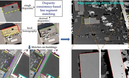
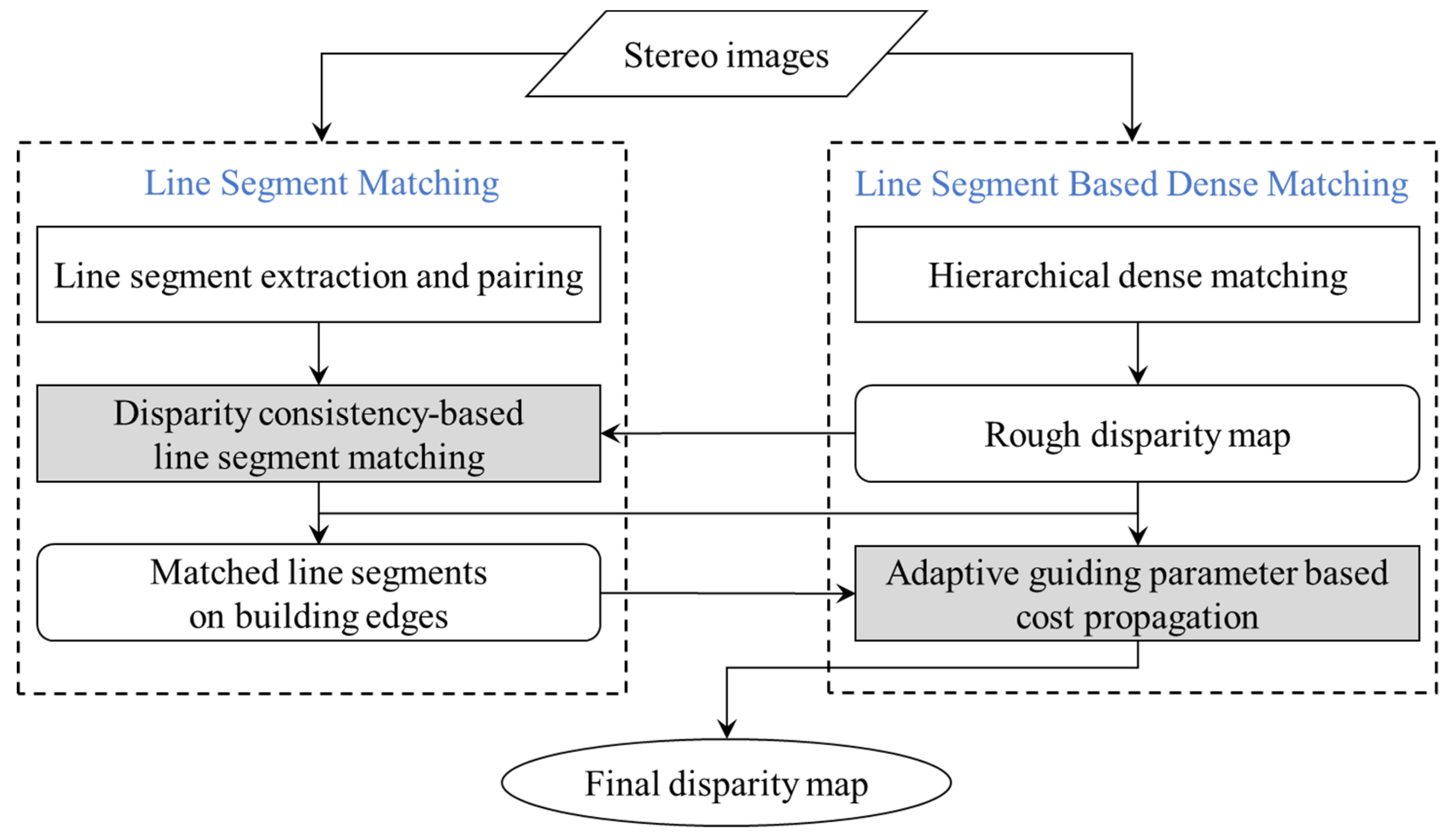
3. Methodology
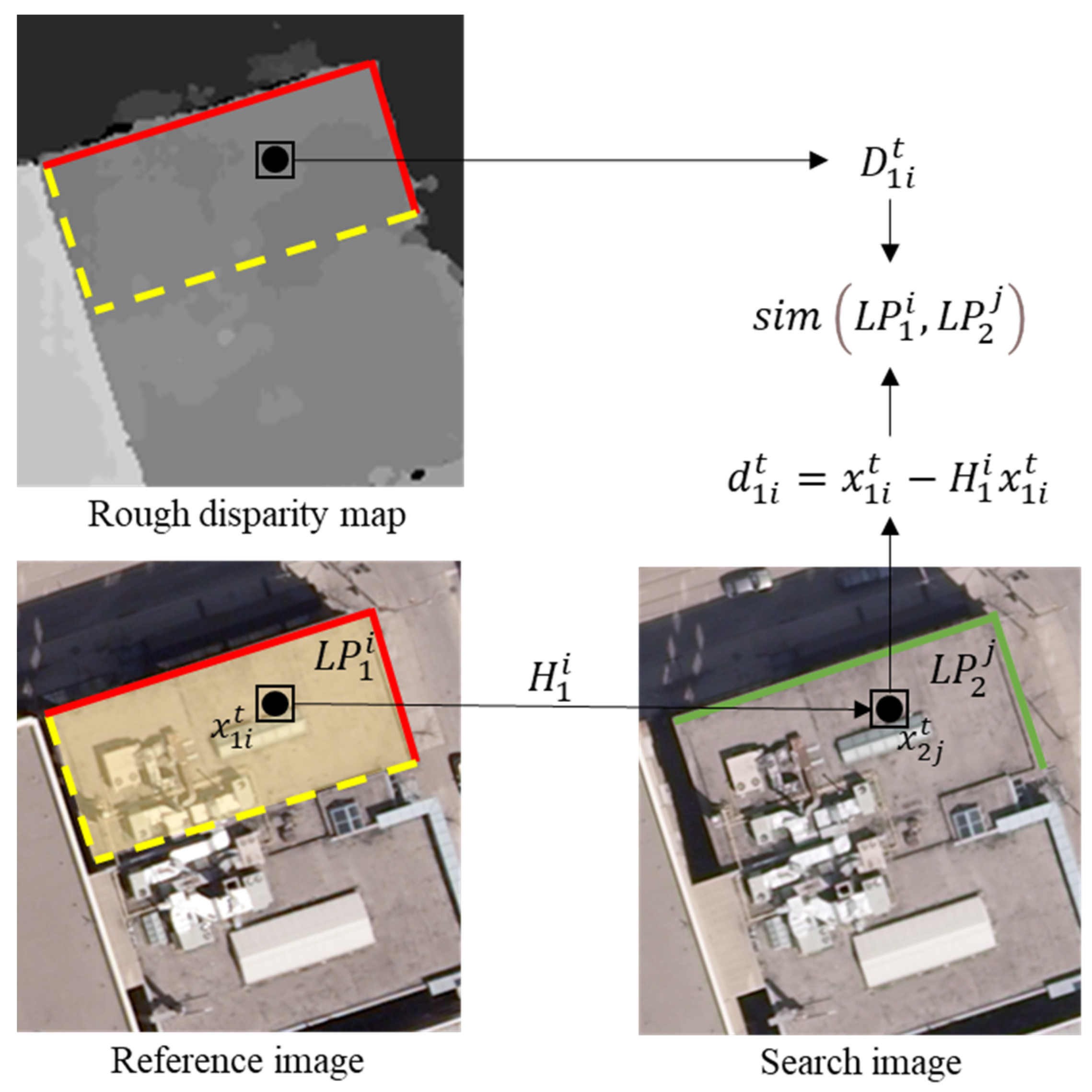
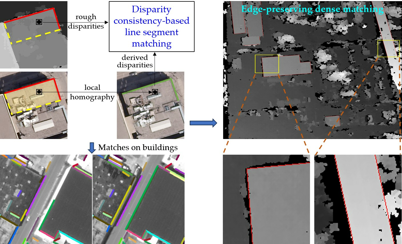
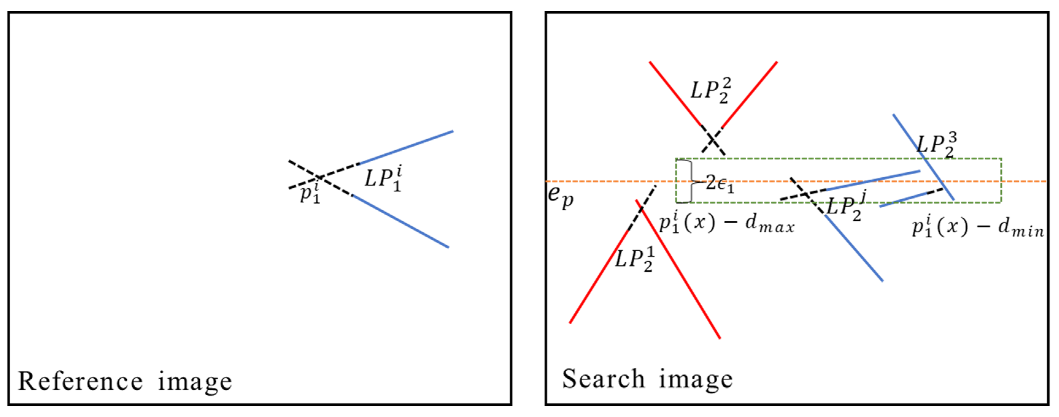
3.1. Disparity Consistency-Based Line Segment Matching
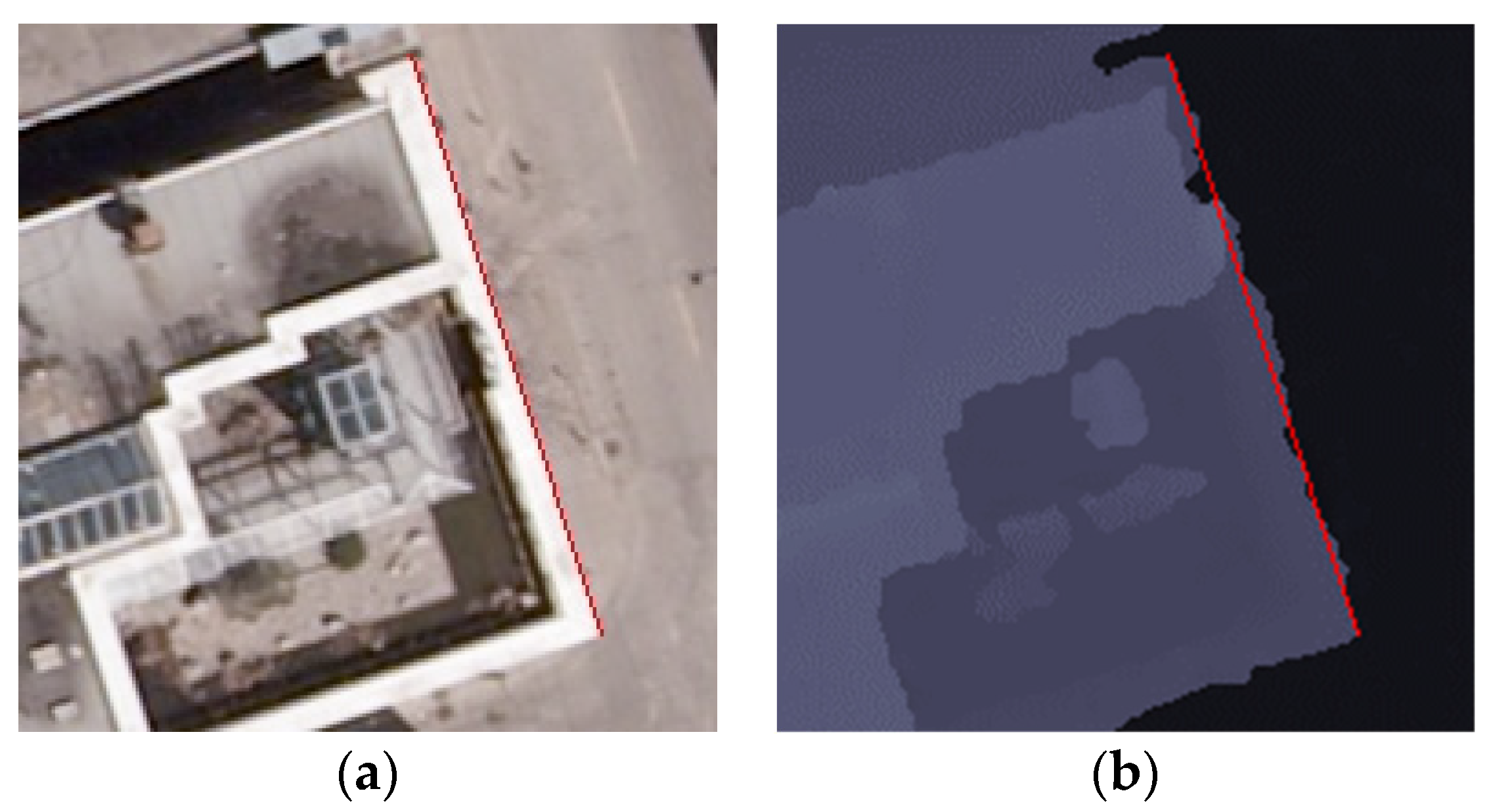
3.2. Line Segment Constrained Dense Matching
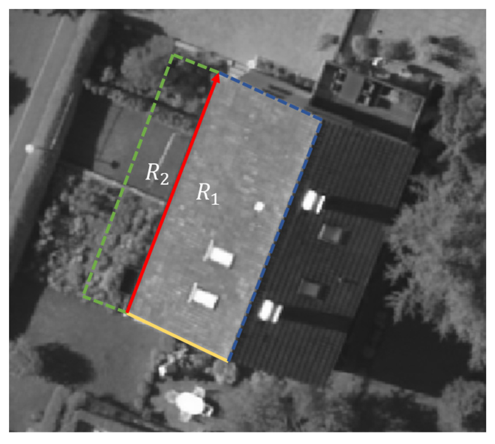
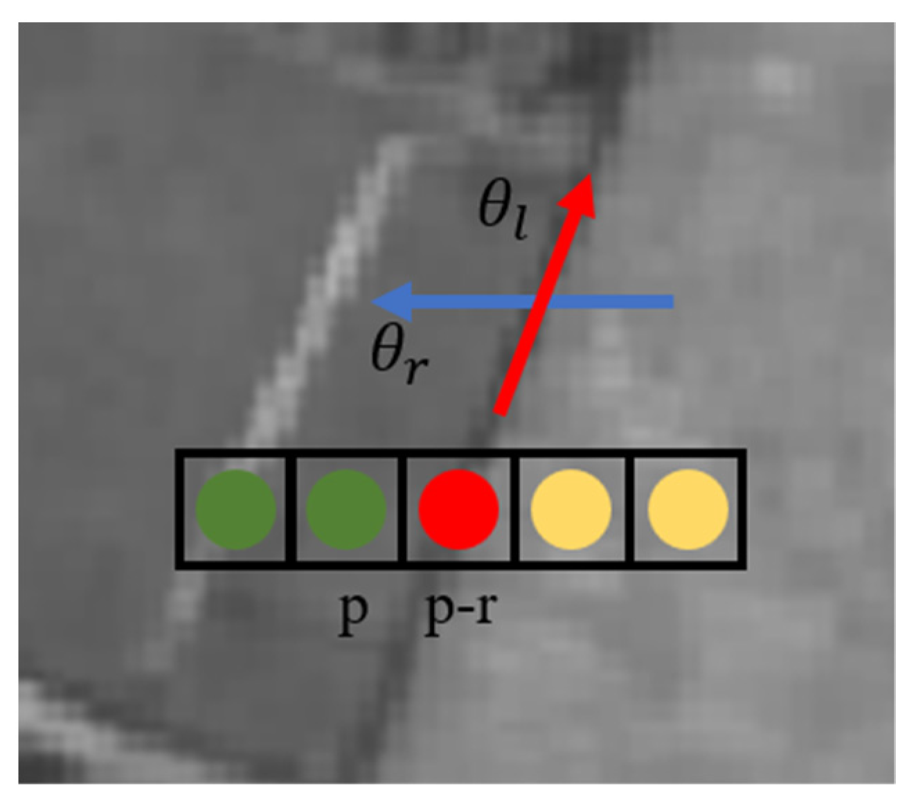
3.2.1. Direction of Line Segments in Discontinuous Areas
3.2.2. Adaptive Guiding Parameter for Cost Propagation
4. Experimental Results and Analysis
4.1. Experimental Datasets
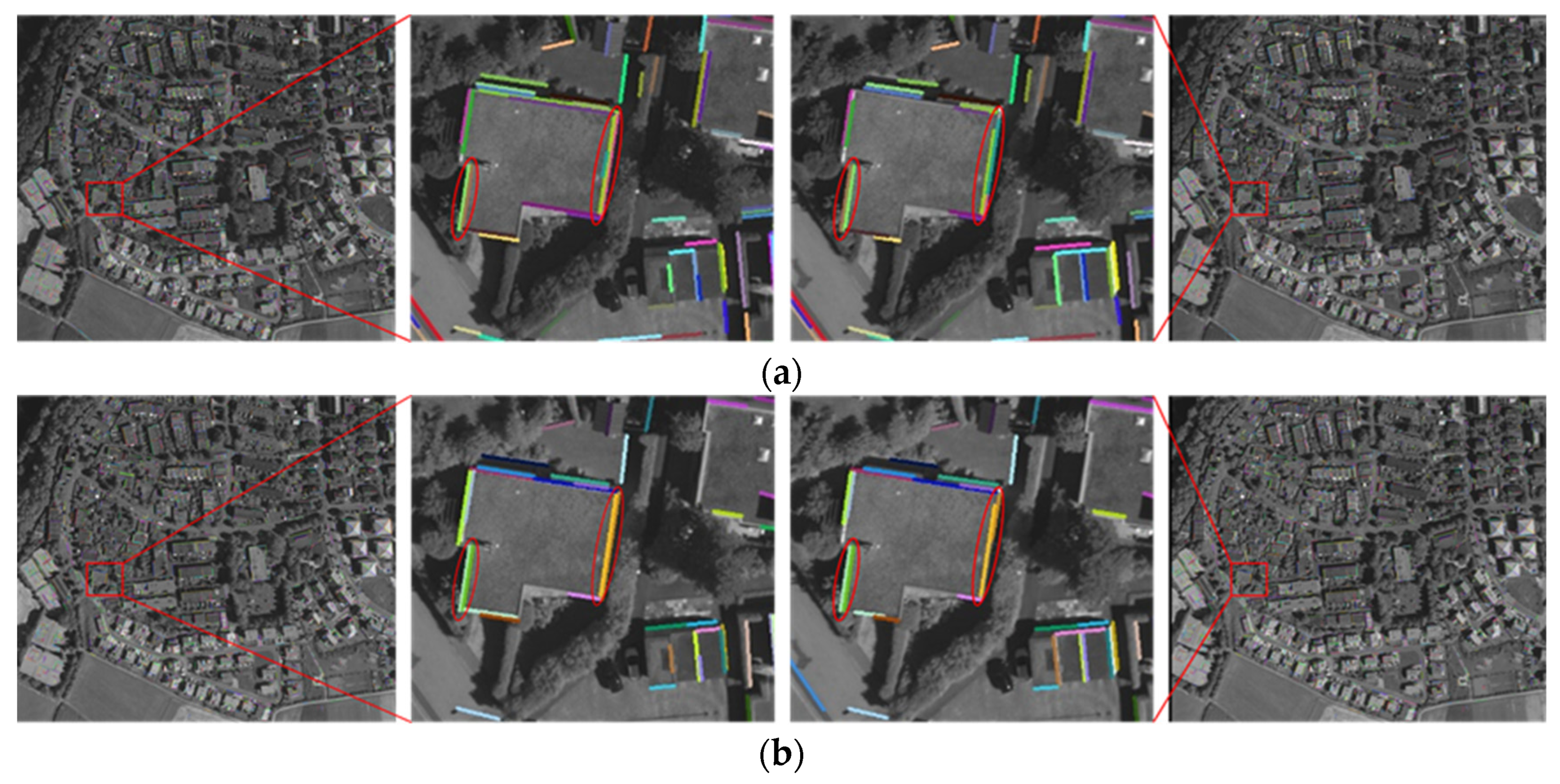
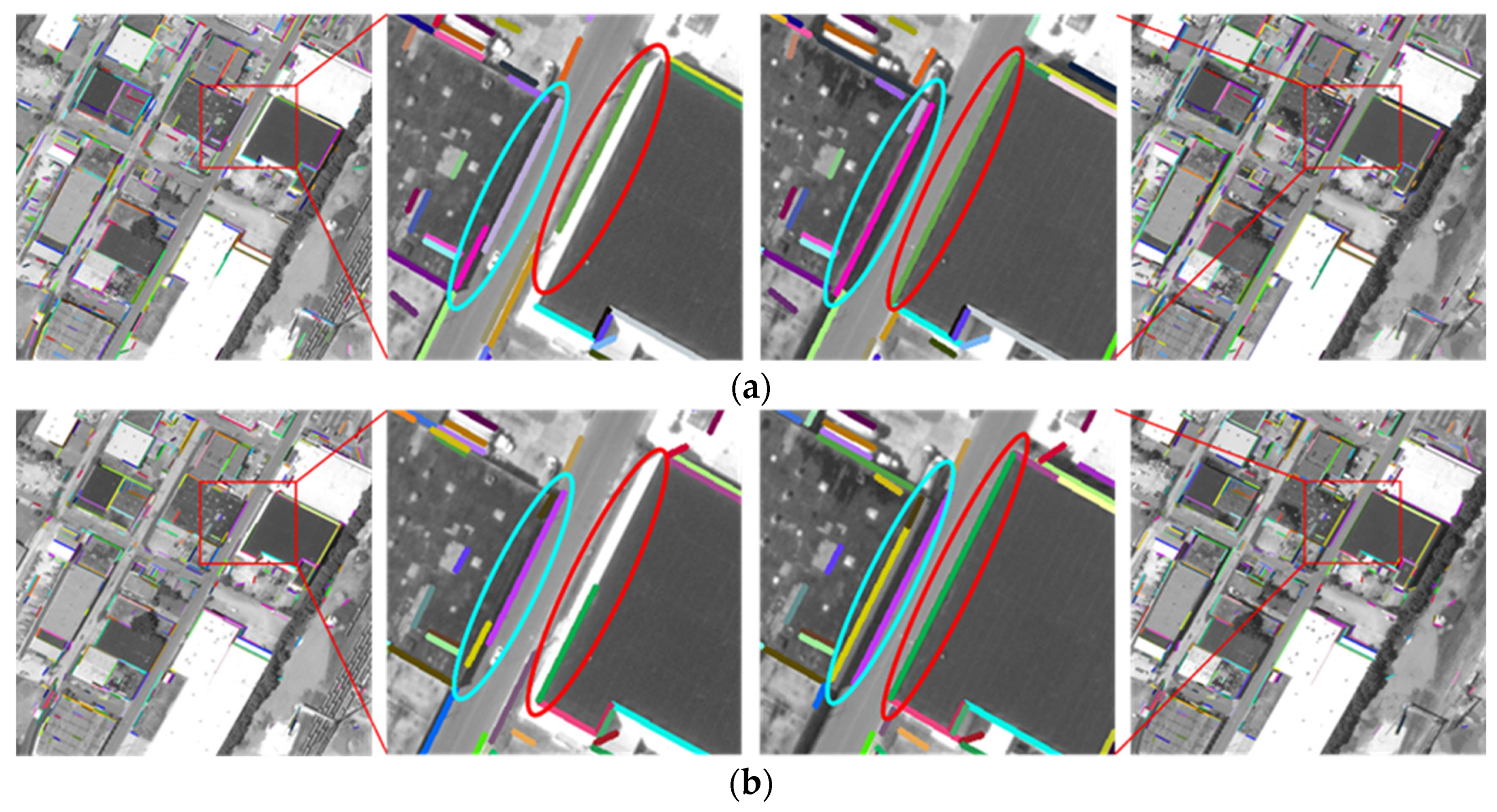
4.2. Evaluation of Line Segment Matching
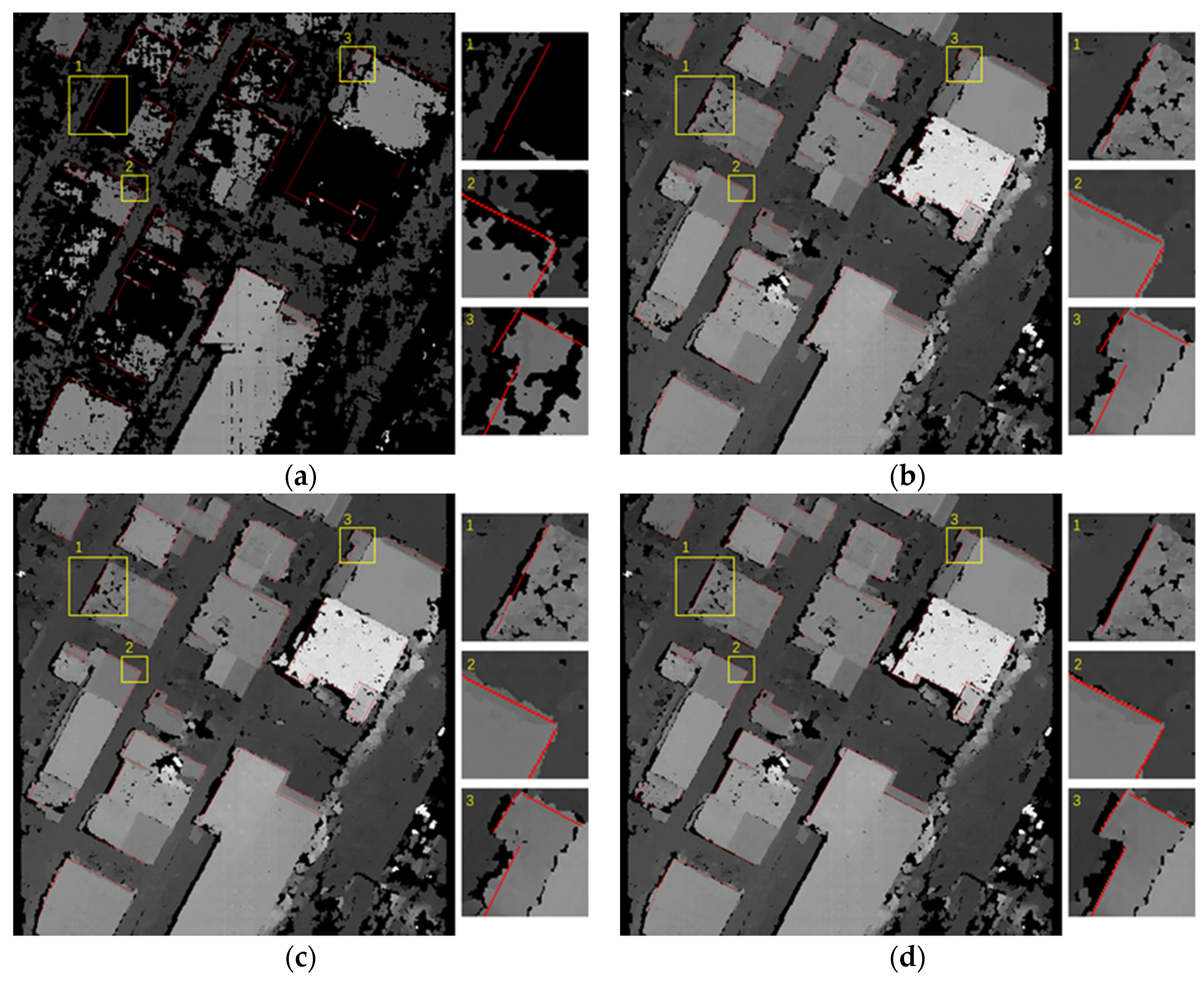
4.3. Evaluation of Line Segment Constrained Dense Matching
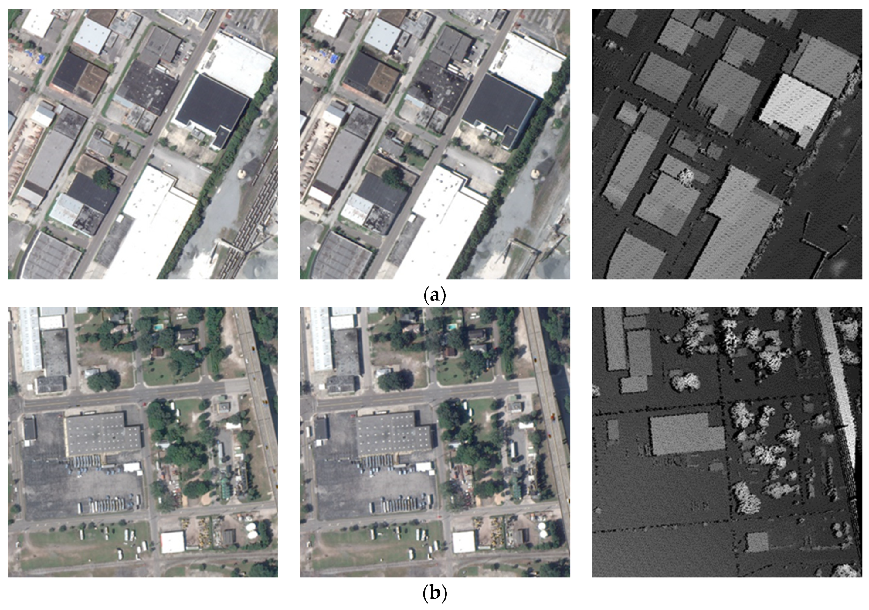
4.3.1. Performance on Satellite Imagery
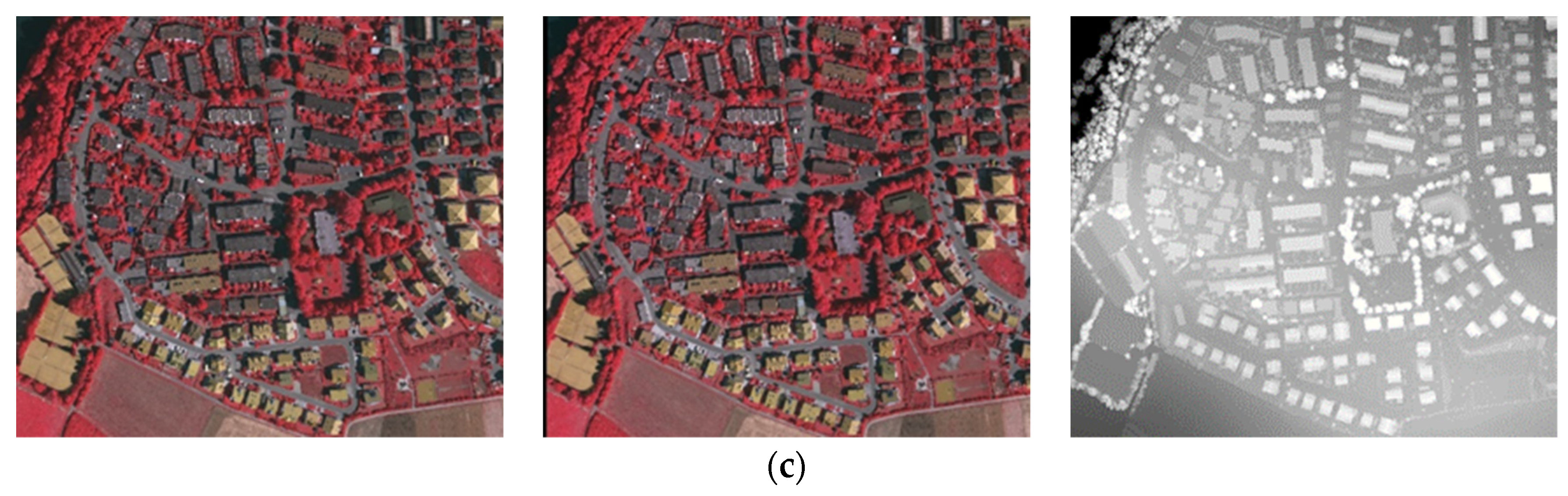
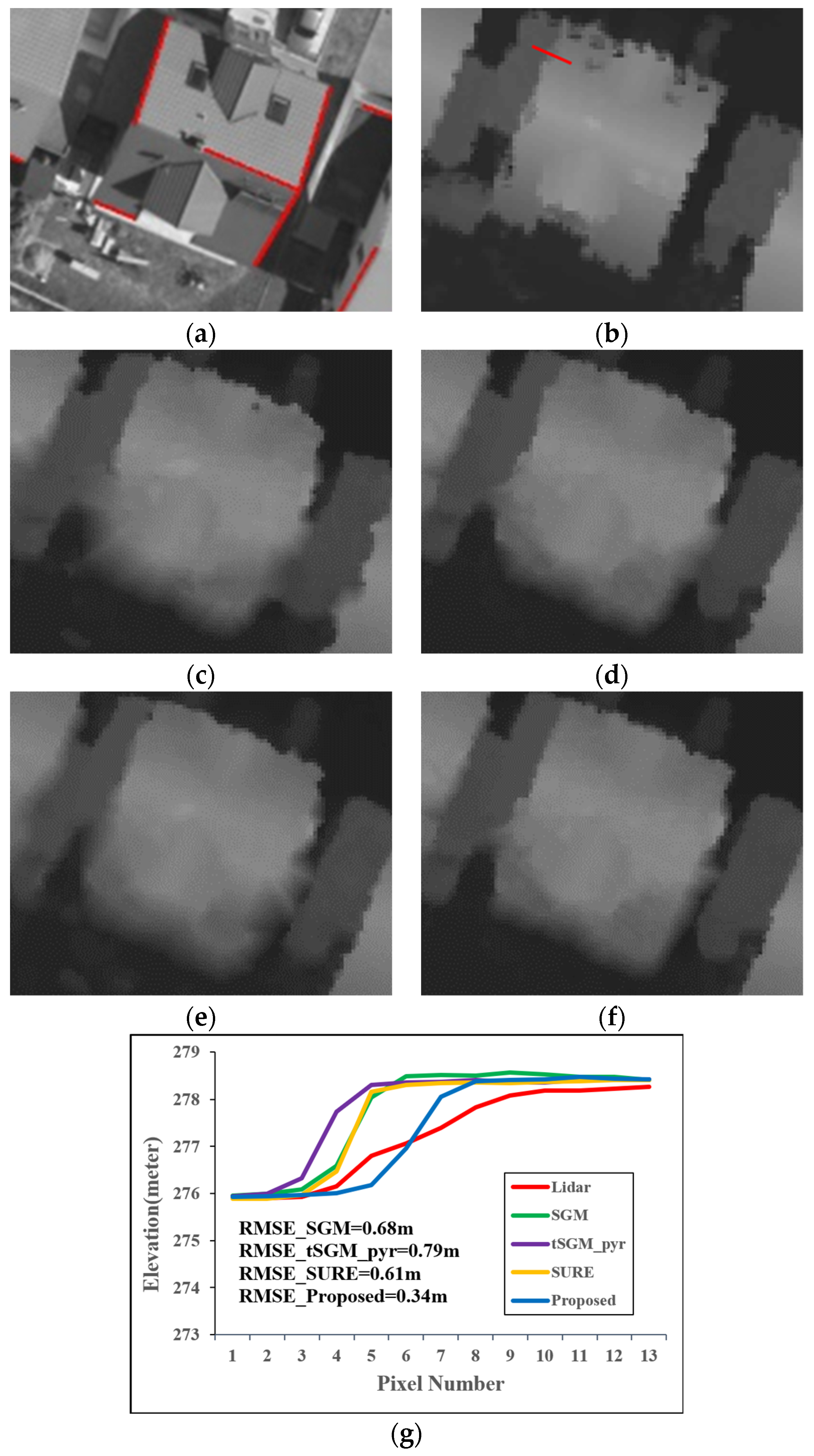
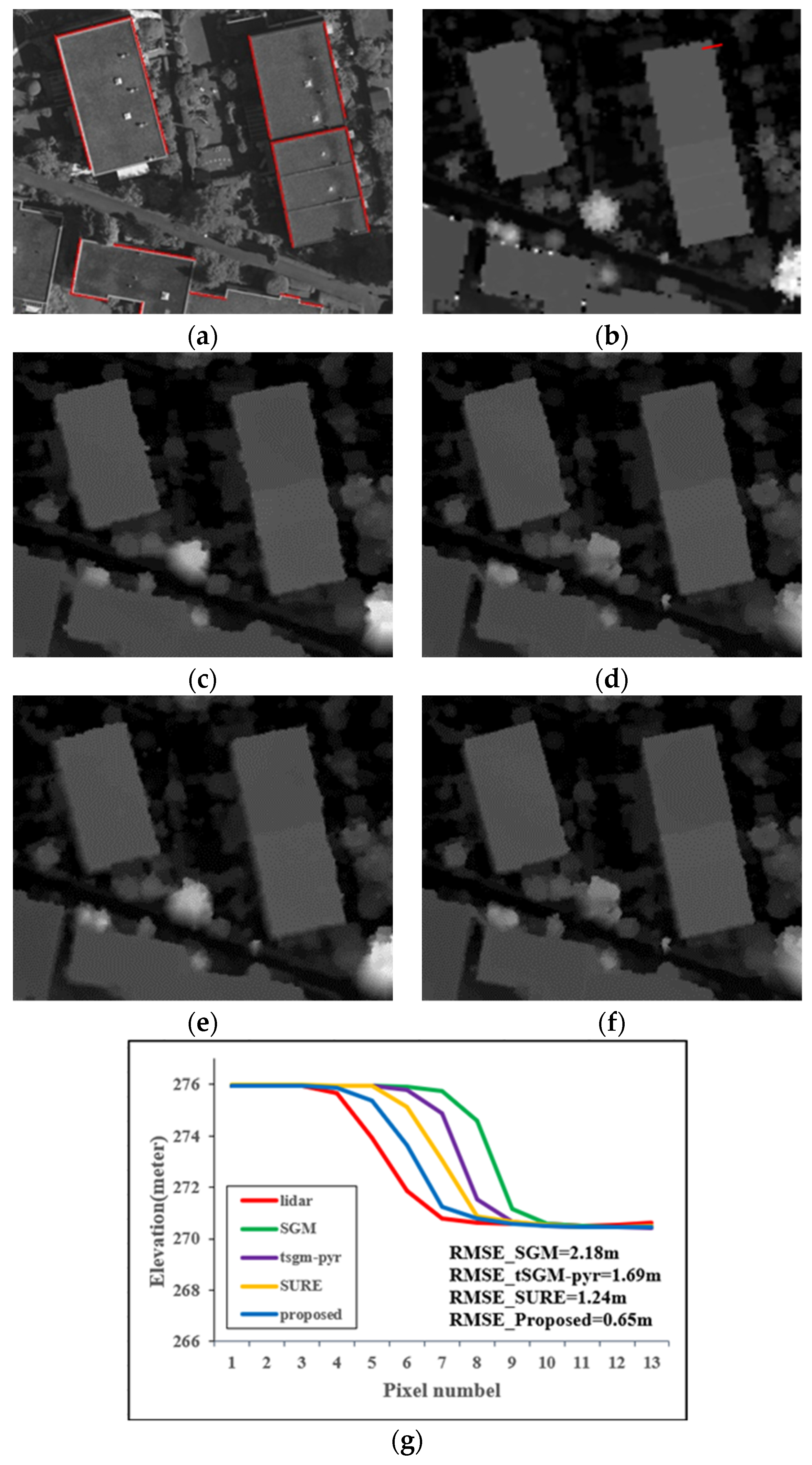
4.3.2. Performance on Aerial Imagery
5. Conclusions
Author Contributions
Funding
Data Availability Statement
Conflicts of Interest
References
- Braun, C.; Kolbe, T.H.; Lang, F.; Schickler, W.; Steinhage, V.; Cremers, A.B.; Förstner, W.; Plümer, L. Models for photogrammetric building reconstruction. Comput. Graph. 1995, 19, 109–118. [Google Scholar] [CrossRef]
- Brenner, C. Building reconstruction from images and laser scanning. Int. J. Appl. Earth Obs. Geoinf. 2005, 6, 187–198. [Google Scholar] [CrossRef]
- Haala, N.; Kada, M. An update on automatic 3D building reconstruction. ISPRS J. Photogramm. Remote Sens. 2010, 65, 570–580. [Google Scholar] [CrossRef]
- Yu, D.; Ji, S.; Liu, J.; Wei, S. Automatic 3D building reconstruction from multi-view aerial images with deep learning. ISPRS J. Photogramm. Remote Sens. 2021, 171, 155–170. [Google Scholar] [CrossRef]
- Gupta, G.; Balasubramanian, R.; Rawat, M.; Bhargava, R.; Gopala Krishna, B. Stereo matching for 3d building reconstruction. In Proceedings of the Advances in Computing, Communication and Control: International Conference, ICAC3 2011, Mumbai, India, 28–29 January 2011; pp. 522–529. [Google Scholar]
- Hamzah, R.A.; Kadmin, A.F.; Hamid, M.S.; Ghani, S.F.A.; Ibrahim, H. Improvement of stereo matching algorithm for 3D surface reconstruction. Signal Process. Image Commun. 2018, 65, 165–172. [Google Scholar] [CrossRef]
- Kendall, A.; Martirosyan, H.; Dasgupta, S.; Henry, P.; Kennedy, R.; Bachrach, A.; Bry, A. End-to-end learning of geometry and context for deep stereo regression. In Proceedings of the IEEE International Conference on Computer Vision, Venice, Italy, 22–29 October 2017; pp. 66–75. [Google Scholar]
- Scharstein, D.; Szeliski, R. A taxonomy and evaluation of dense two-frame stereo correspondence algorithms. Int. J. Comput. Vis. 2002, 47, 7–42. [Google Scholar] [CrossRef]
- Hirschmuller, H. Accurate and efficient stereo processing by semi-global matching and mutual information. In Proceedings of the 2005 IEEE Computer Society Conference on Computer Vision and Pattern Recognition (CVPR’05), San Diego, CA, USA, 20–25 June 2005; pp. 807–814. [Google Scholar]
- Hirschmuller, H. Stereo processing by semiglobal matching and mutual information. IEEE Trans. Pattern Anal. Mach. Intell. 2007, 30, 328–341. [Google Scholar] [CrossRef] [PubMed]
- Facciolo, G.; De Franchis, C.; Meinhardt, E. MGM: A significantly more global matching for stereovision. In Proceedings of the BMVC 2015, Swansea, UK, 7–10 September 2015. [Google Scholar]
- Patil, S.; Prakash, T.; Comandur, B.; Kak, A. A comparative evaluation of SGM variants (including a new variant, tMGM) for dense stereo matching. arXiv 2019, arXiv:1911.09800. [Google Scholar]
- Scharstein, D.; Taniai, T.; Sinha, S.N. Semi-global stereo matching with surface orientation priors. In Proceedings of the 2017 International Conference on 3D Vision (3DV), Qingdao, China, 10–12 October 2017; pp. 215–224. [Google Scholar]
- Rothermel, M.; Wenzel, K.; Fritsch, D.; Haala, N. SURE: Photogrammetric surface reconstruction from imagery. In Proceedings of the LC3D Workshop, Berlin, Germany, 4–5 December 2012. [Google Scholar]
- Chuang, T.-Y.; Ting, H.-W.; Jaw, J.-J. Dense stereo matching with edge-constrained penalty tuning. IEEE Geosci. Remote Sens. Lett. 2018, 15, 664–668. [Google Scholar] [CrossRef]
- Kim, K.-R.; Kim, C.-S. Adaptive smoothness constraints for efficient stereo matching using texture and edge information. In Proceedings of the 2016 IEEE International Conference on Image Processing (ICIP), Phoenix, AZ, USA, 25–28 September 2016; pp. 3429–3433. [Google Scholar]
- Kim, G.-B.; Chung, S.-C. An accurate and robust stereo matching algorithm with variable windows for 3D measurements. Mechatronics 2004, 14, 715–735. [Google Scholar] [CrossRef]
- Xu, Y.; Zhao, Y.; Ji, M. Local stereo matching with adaptive shape support window based cost aggregation. Appl. Opt. 2014, 53, 6885–6892. [Google Scholar] [CrossRef] [PubMed]
- Zhu, S.; Yan, L. Local stereo matching algorithm with efficient matching cost and adaptive guided image filter. Vis. Comput. 2017, 33, 1087–1102. [Google Scholar] [CrossRef]
- Chen, D.; Ardabilian, M.; Chen, L. A Novel Trilateral Filter based Adaptive Support Weight Method for Stereo Matching. In Proceedings of the BMVC, Bristol, UK, 9–13 September 2013. [Google Scholar]
- Hosni, A.; Rhemann, C.; Bleyer, M.; Rother, C.; Gelautz, M. Fast cost-volume filtering for visual correspondence and beyond. IEEE Trans. Pattern Anal. Mach. Intell. 2012, 35, 504–511. [Google Scholar] [CrossRef] [PubMed]
- Tatar, N.; Arefi, H.; Hahn, M. High-resolution satellite stereo matching by object-based semiglobal matching and iterative guided edge-preserving filter. IEEE Geosci. Remote Sens. Lett. 2020, 18, 1841–1845. [Google Scholar] [CrossRef]
- Cheng, F.; Zhang, H.; Yuan, D.; Sun, M. Stereo matching by using the global edge constraint. Neurocomputing 2014, 131, 217–226. [Google Scholar] [CrossRef]
- Huang, X.; Zhang, Y.; Yue, Z. Image-Guided Non-Local Dense Matching with Three-Steps Optimization. ISPRS Ann. Photogramm. Remote Sens. Spat. Inf. Sci. 2016, 3, 67–74. [Google Scholar] [CrossRef]
- Jiao, J.; Wang, R.; Wang, W.; Li, D.; Gao, W. Color image-guided boundary-inconsistent region refinement for stereo matching. IEEE Trans. Circuits Syst. Video Technol. 2015, 27, 1155–1159. [Google Scholar] [CrossRef]
- Qin, R.; Chen, M.; Huang, X.; Hu, K. Disparity refinement in depth discontinuity using robustly matched straight lines for digital surface model generation. IEEE J. Sel. Top. Appl. Earth Obs. Remote Sens. 2018, 12, 174–185. [Google Scholar] [CrossRef]
- Schmid, C.; Zisserman, A. Automatic line matching across views. In Proceedings of the IEEE Computer Society Conference on Computer Vision and Pattern Recognition, San Juan, PR, USA, 17–19 June 1997; pp. 666–671. [Google Scholar]
- Wang, Z.; Wu, F.; Hu, Z. MSLD: A robust descriptor for line matching. Pattern Recognit. 2009, 42, 941–953. [Google Scholar] [CrossRef]
- Chen, M.; Li, W.; Fang, T.; Zhu, Q.; Xu, B.; Hu, H.; Ge, X. An adaptive feature region-based line segment matching method for viewpoint-changed images with discontinuous parallax and poor textures. Int. J. Appl. Earth Obs. Geoinf. 2023, 117, 103209. [Google Scholar] [CrossRef]
- Chen, M.; Yan, S.; Qin, R.; Zhao, X.; Fang, T.; Zhu, Q.; Ge, X. Hierarchical line segment matching for wide-baseline images via exploiting viewpoint robust local structure and geometric constraints. ISPRS J. Photogramm. Remote Sens. 2021, 181, 48–66. [Google Scholar] [CrossRef]
- Li, K.; Yao, J. Line segment matching and reconstruction via exploiting coplanar cues. ISPRS J. Photogramm. Remote Sens. 2017, 125, 33–49. [Google Scholar] [CrossRef]
- Von Gioi, R.G.; Jakubowicz, J.; Morel, J.-M.; Randall, G. LSD: A fast line segment detector with a false detection control. IEEE Trans. Pattern Anal. Mach. Intell. 2010, 32, 722–732. [Google Scholar] [CrossRef] [PubMed]
- Hartley, R.; Zisserman, A. Multiple View Geometry in Computer Vision; Cambridge University Press: Cambridge, UK, 2003. [Google Scholar]
- Bosch, M.; Foster, K.; Christie, G.; Wang, S.; Hager, G.D.; Brown, M. Semantic stereo for incidental satellite images. In Proceedings of the 2019 IEEE Winter Conference on Applications of Computer Vision (WACV), Waikoloa Village, HI, USA, 7–11 January 2019; pp. 1524–1532. [Google Scholar]
- Available online: https://www.isprs.org/education/benchmarks/UrbanSemLab/detection-and-reconstruction.aspx (accessed on 11 August 2022).
- Canny, J. A computational approach to edge detection. IEEE Trans. Pattern Anal. Mach. Intell. 1986, 6, 679–698. [Google Scholar] [CrossRef]
- Scharstein, D.; Szeliski, R. Middlebury Online Sstereo Evaluation. 2023. Available online: https://vision.middlebury.edu/stereo/ (accessed on 22 August 2022).


| Dataset | NCM | MP (%) | ET (s) | ||||||
|---|---|---|---|---|---|---|---|---|---|
| MSLD | LJL | Proposed | MSLD | LJL | Proposed | MSLD | LJL | Proposed | |
| Pair 1 | 97 | 380 | 362 | 83.5 | 83.5 | 97.5 | 0.7 | 225 | 3 |
| Pair 3 | 1814 | 2536 | 2528 | 94.6 | 93.3 | 99.4 | 11.5 | 3910 | 52 |
| Method | IPE (%) | OPE (%) | BPE (%) | TE (%) |
|---|---|---|---|---|
| SGM | 57.80 | 2.49 | 3.91 | 64.20 |
| tSGM-pyr | 7.67 | 12.77 | 19.16 | 39.60 |
| tSGM | 6.87 | 12.64 | 18.71 | 38.22 |
| Proposed | 8.14 | 10.17 | 15.96 | 34.26 |
| Method | RMSE (m) | BPE (%) |
|---|---|---|
| SGM | 1.91 | 25.80 |
| tSGM-pyr | 1.88 | 25.10 |
| tSGM | 1.73 | 22.24 |
| Proposed | 1.65 | 20.51 |
Disclaimer/Publisher’s Note: The statements, opinions and data contained in all publications are solely those of the individual author(s) and contributor(s) and not of MDPI and/or the editor(s). MDPI and/or the editor(s) disclaim responsibility for any injury to people or property resulting from any ideas, methods, instructions or products referred to in the content. |
© 2023 by the authors. Licensee MDPI, Basel, Switzerland. This article is an open access article distributed under the terms and conditions of the Creative Commons Attribution (CC BY) license (https://creativecommons.org/licenses/by/4.0/).
Share and Cite
Yue, Y.; Fang, T.; Li, W.; Chen, M.; Xu, B.; Ge, X.; Hu, H.; Zhang, Z. Hierarchical Edge-Preserving Dense Matching by Exploiting Reliably Matched Line Segments. Remote Sens. 2023, 15, 4311. https://doi.org/10.3390/rs15174311
Yue Y, Fang T, Li W, Chen M, Xu B, Ge X, Hu H, Zhang Z. Hierarchical Edge-Preserving Dense Matching by Exploiting Reliably Matched Line Segments. Remote Sensing. 2023; 15(17):4311. https://doi.org/10.3390/rs15174311
Chicago/Turabian StyleYue, Yi, Tong Fang, Wen Li, Min Chen, Bo Xu, Xuming Ge, Han Hu, and Zhanhao Zhang. 2023. "Hierarchical Edge-Preserving Dense Matching by Exploiting Reliably Matched Line Segments" Remote Sensing 15, no. 17: 4311. https://doi.org/10.3390/rs15174311
APA StyleYue, Y., Fang, T., Li, W., Chen, M., Xu, B., Ge, X., Hu, H., & Zhang, Z. (2023). Hierarchical Edge-Preserving Dense Matching by Exploiting Reliably Matched Line Segments. Remote Sensing, 15(17), 4311. https://doi.org/10.3390/rs15174311