


Assimilation of ASCAT Radar Backscatter Coefficients over Southwestern France
 ,
,  ,
, 
Abstract
:
1. Introduction
2. Materials and Methods
2.1. The ISBA LSM
- 14 layers for soil temperature, down to 12 m (0–0.01 m, 0.01–0.04 m, 0.04–0.10 m, 0.1–0.2 m, 0.2–0.4 m), 0.4–0.6 m, 0.6–0.8 m, 0.8–1.0 m, 1.0–1.5 m, 1.5–2.0 m, 2–3 m, 3–5 m, 5–8 m and 8–12 m)
- 8 to 10 layers for soil moisture (same depths as for soil temperature), down to 1 m and 2 m depending on vegetation characteristics.
2.2. LDAS-Monde
2.3. ASCAT Data
2.4. LAI Data
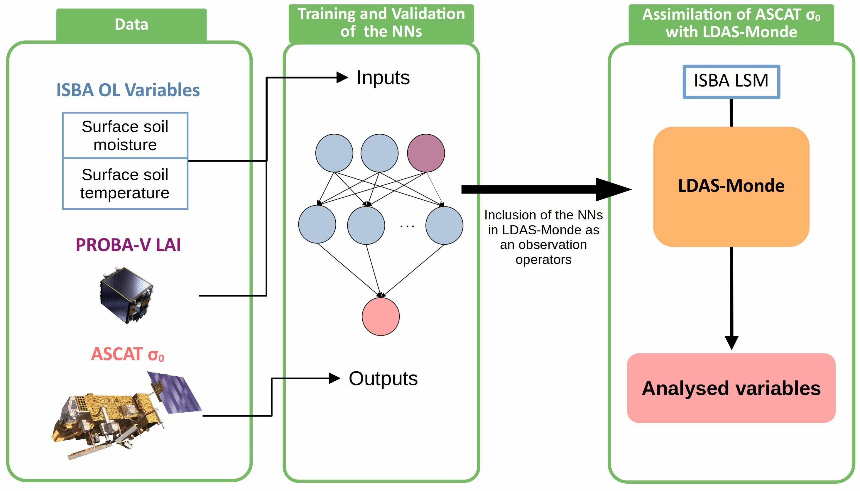
2.5. Observation Operator Based on Neural Networks
- Model soil moisture for the 0.01–0.04 m layer (WG2).
- Model soil temperature for the same layer.
- PROBA-V LAI provided by CGLS.
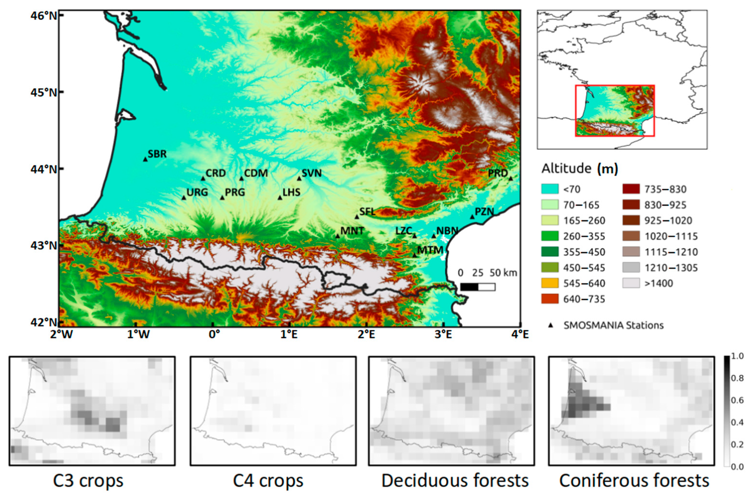
2.6. In Situ Soil Moisture Observations
2.7. Experimental Setup and Assessment
- Open loop (OL), a 12-year ISBA run without assimilation performed after a 20-fold spin-up of the initial year—2007.
- A 4-year conventional simplified extended Kalman filter analysis based on the assimilation of the ASCAT SWI-001 product and LAI (EKF_SWI_LAI).
- A novel configuration based on the assimilation of σ040 (EKF).
3. Results
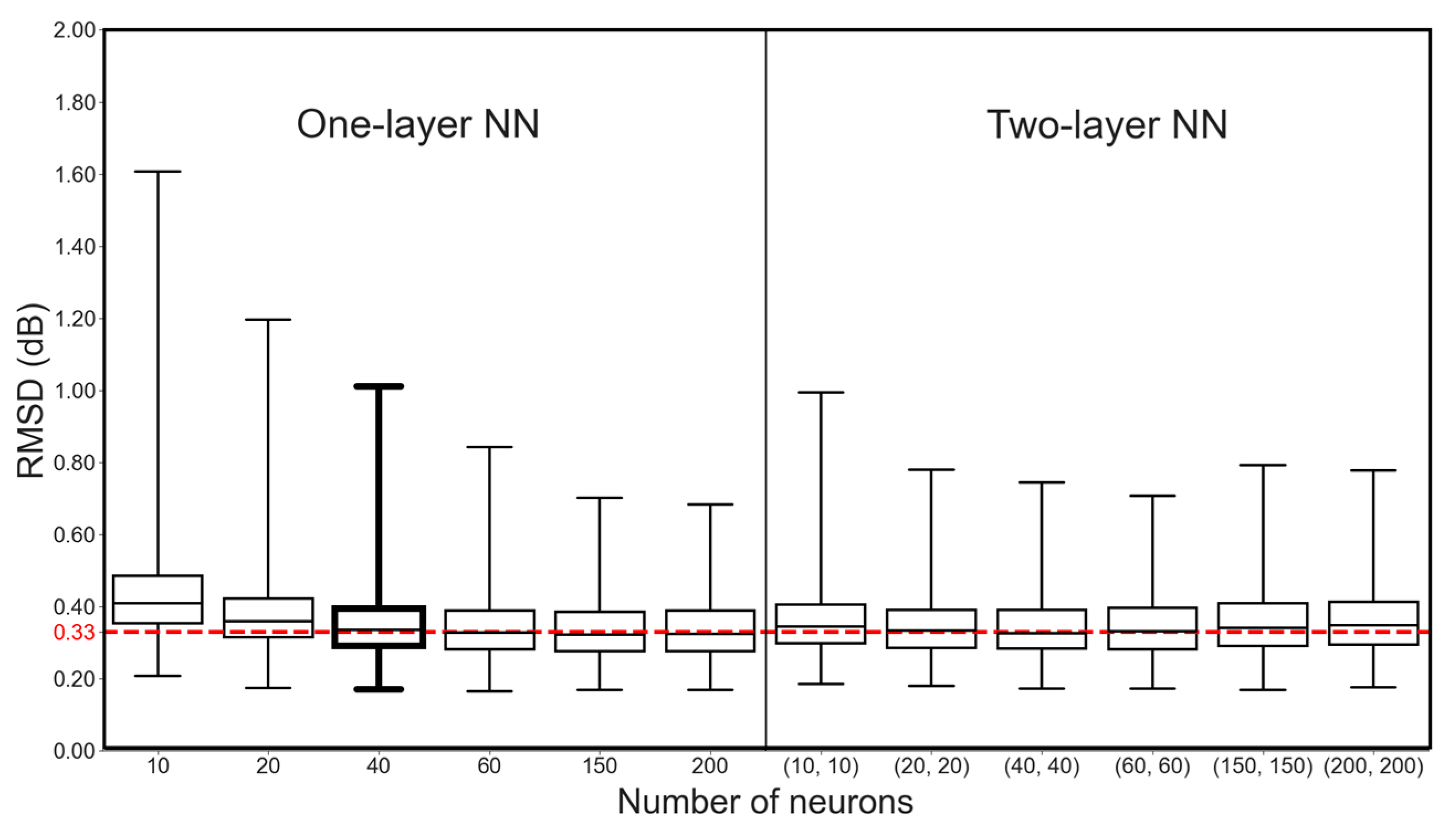
3.1. NN Training and Architecture Selection
3.2. NN Predictor Sensitivity
3.3. NN Validation
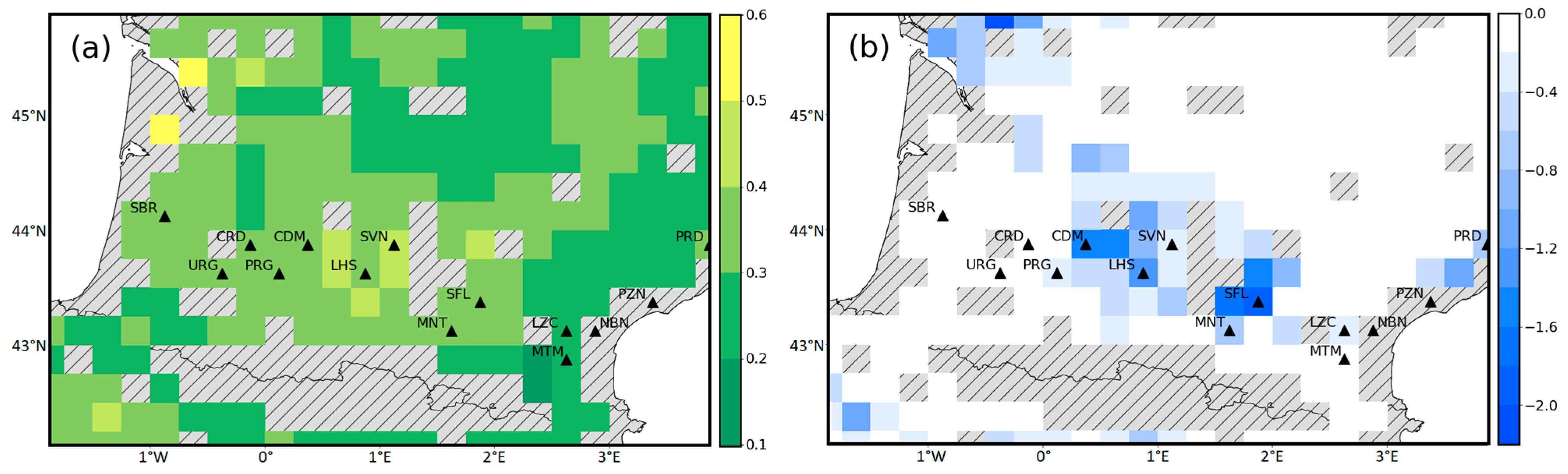
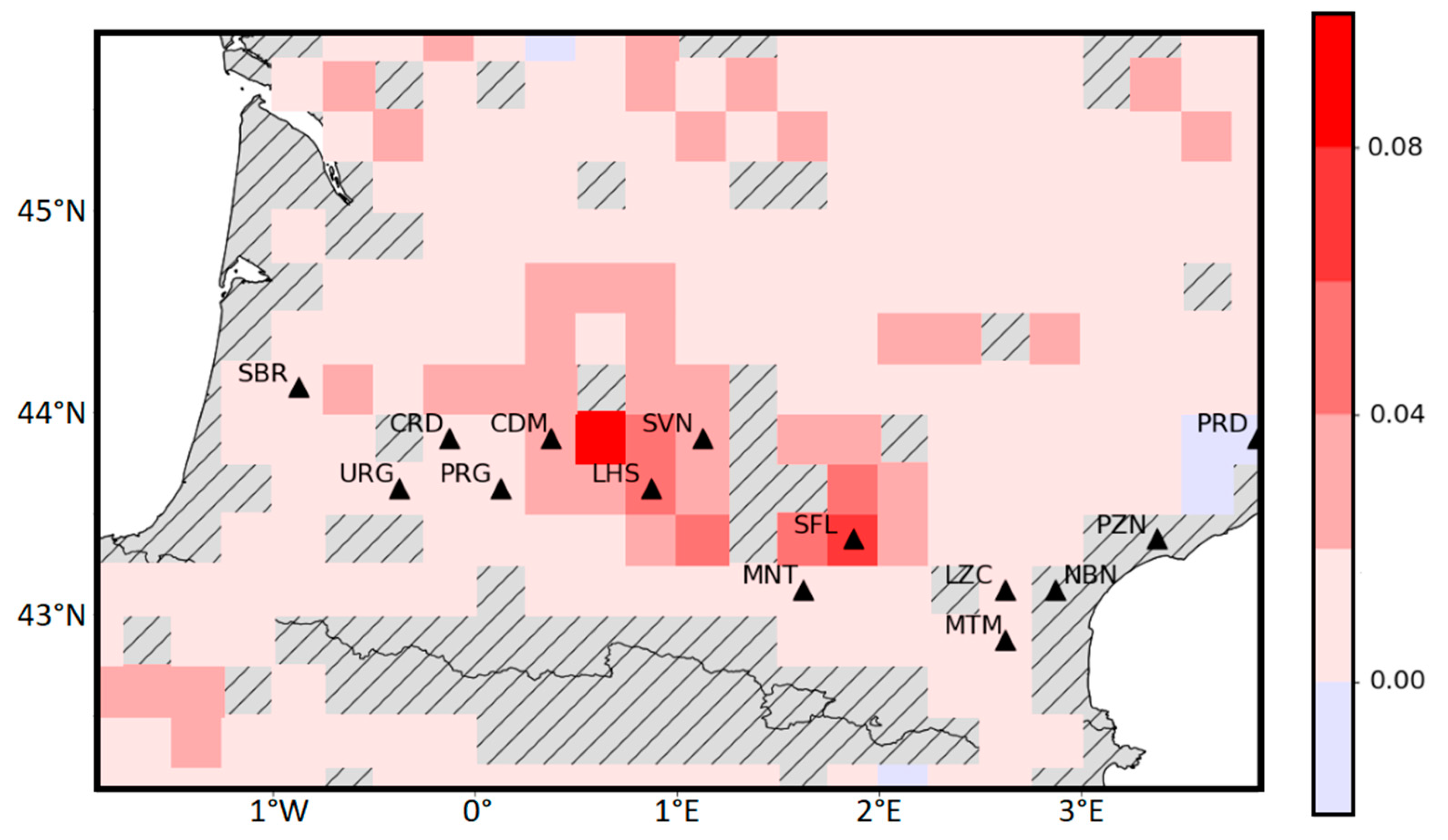
3.4. Impact of Assimilating σ040 Observations
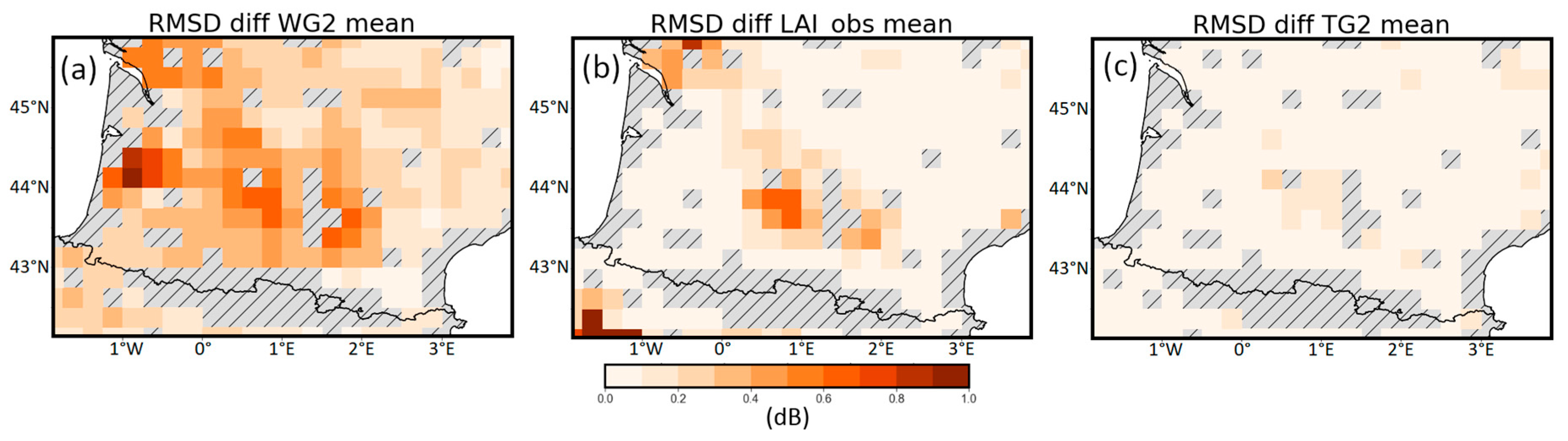
3.4.1. Simulated σ040
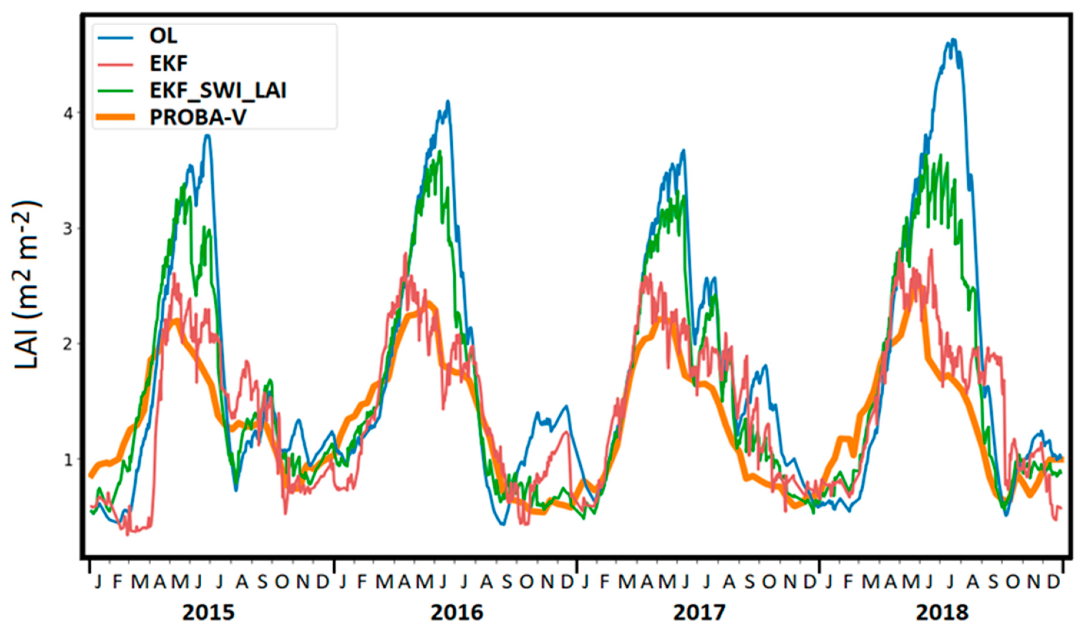
3.4.2. Simulated LAI
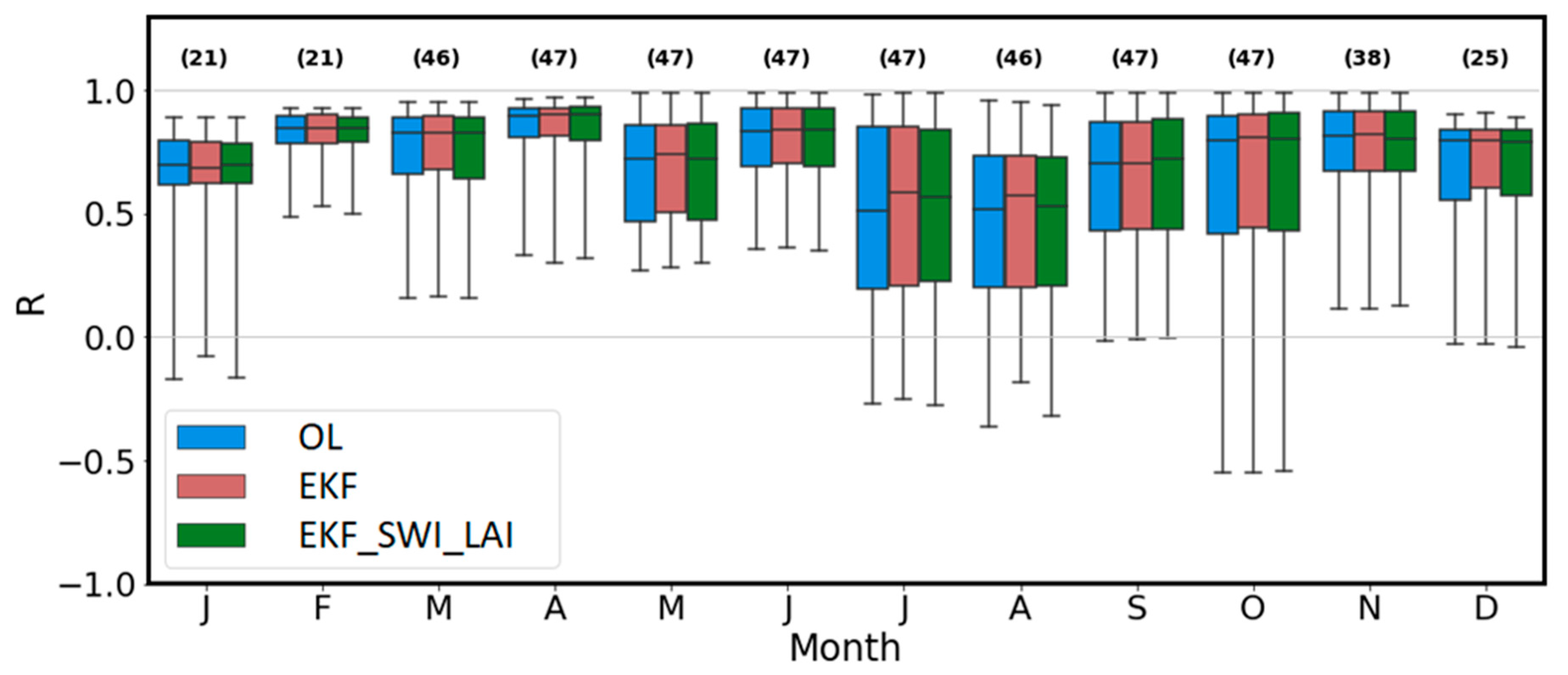
3.4.3. Simulated SSM
4. Discussion
4.1. Assimilating Microwave Retrievals or Radiance?
4.2. What Are the Biophysical Drivers of ASCAT σ040?
4.3. Assimilating Microwave Radiance or LAI?
5. Conclusions
Author Contributions
Funding
Data Availability Statement
Acknowledgments
Conflicts of Interest
References
- Samaniego, L.; Thober, S.; Kumar, R.; Wanders, N.; Rakovec, O.; Pan, M.; Zink, M.; Sheffield, J.; Wood, E.F.; Marx, A. Anthropogenic Warming Exacerbates European Soil Moisture Droughts. Nat. Clim. Chang. 2018, 8, 421–426. [Google Scholar] [CrossRef]
- Grillakis, M.G. Increase in severe and extreme soil moisture droughts for Europe under climate change. Sci. Total Environ. 2019, 660, 1245–1255. [Google Scholar] [CrossRef] [PubMed]
- Spinoni, J.; Naumann, G.; Carrao, H.; Barbosa, P.; Vogt, J. World drought frequency, duration, and severity for 1951–2010. Int. J. Climatol. 2014, 34, 2792–2804. [Google Scholar] [CrossRef]
- Di Napoli, C.; Pappenberger, F.; Cloke, H.L. Verification of heat stress thresholds for a health-based heatwave definition. J. Appl. Meteorol. Climatol. 2019, 58, 1177–1194. [Google Scholar] [CrossRef]
- Beillouin, D.; Schauberger, B.; Bastos, A.; Ciais, P.; Makowski, D. Impact of extreme weather conditions on European crop production in 2018. Philos. Trans. R. Soc. B 2020, 375, 20190510. [Google Scholar] [CrossRef] [PubMed]
- Wagner, W.; Lemoine, G.; Rott, H. A method for estimating soil moisture from ERS scatterometer and soil data. Remote Sens. Environ. 1999, 70, 191–207. [Google Scholar] [CrossRef]
- Muñoz-Sabater, J.; Dutra, E.; Agustí-Panareda, A.; Albergel, C.; Arduini, G.; Balsamo, G.; Boussetta, S.; Choulga, M.; Harrigan, S.; Hersbach, H.; et al. ERA5-Land: A state-of-the-art global reanalysis dataset for land applications. Earth Syst. Sci. Data 2021, 13, 4349–4383. [Google Scholar] [CrossRef]
- Balsamo, G.; Albergel, C.; Beljaars, A.; Boussetta, S.; Brun, E.; Cloke, H.; Dee, D.; Dutra, E. ERA-Interim/Land: A global land surface reanalysis data set. Hydrol. Earth Syst. Sci. 2015, 19, 389–407. [Google Scholar] [CrossRef]
- Balsamo, G.; Agustì-parareda, A.; Albergel, C.; Arduini, G.; Beljaars, A.; Bidlot, J.; Blyth, E.; Bousserez, N.; Boussetta, S.; Brown, A.; et al. Satellite and in situ observations for advancing global Earth surface modelling: A review. Remote Sens. 2018, 10, 2038. [Google Scholar] [CrossRef]
- Mucia, A.; Bonan, B.; Zheng, Y.; Albergel, C.; Calvet, J.-C. From monitoring to forecasting land surface conditions using a land data assimilation system: Application over the Contiguous United States. Remote Sens. 2020, 12, 2020. [Google Scholar] [CrossRef]
- Rodríguez-Fernández, N.; de Rosnay, P.; Albergel, C.; Richaume, P.; Aires, F.; Prigent, C.; Kerr, Y. SMOS neural network soil moisture data assimilation in a land surface model and atmospheric impact. Remote Sens. 2019, 11, 1334. [Google Scholar] [CrossRef]
- Séférian, R.; Nabat, P.; Michou, M.; Saint-Martin, D.; Voldoire, A.; Colin, J.; Decharme, B.; Delire, C.; Berthet, S.; Chevallier, M.; et al. Evaluation of CNRM Earth system model, CNRM-ESM2-1: Role of Earth system processes in present-day and future climate. J. Adv. Model. Earth Syst. 2019, 11, 4182–4227. [Google Scholar] [CrossRef]
- Kumar, S.; Kolassa, J.; Reichle, R.; Crow, W.; de Lannoy, G.; de Rosnay, P.; MacBean, N.; Girotto, M.; Fox, A.; Quaife, T.; et al. An agenda for land data assimilation priorities: Realizing the promise of terrestrial water, energy, and vegetation observations from space. J. Adv. Model. Earth Syst. 2022, 14, e2022MS003259. [Google Scholar] [CrossRef]
- De Lannoy, G.J.M.; Bechtold, M.; Albergel, C.; Brocca, L.; Calvet, J.-C.; Carrassi, A.; Crow, W.T.; de Rosnay, P.; Durand, M.; Forman, B.; et al. Perspective on satellite-based land data assimilation to estimate water cycle components in an era of advanced data availability and model sophistication. Front. Water 2022, 4, 981745. [Google Scholar] [CrossRef]
- Albergel, C.; Munier, S.; Jennifer Leroux, D.; Dewaele, H.; Fairbairn, D.; Lavinia Barbu, A.; Gelati, E.; Dorigo, W.; Faroux, S.; Meurey, C.; et al. Sequential assimilation of satellite-derived vegetation and soil moisture products using SURFEX-v8.0: LDAS-Monde assessment over the Euro-Mediterranean area. Geosci. Model Dev. 2017, 10, 3889–3912. [Google Scholar] [CrossRef]
- Albergel, C.; Dutra, E.; Munier, S.; Calvet, J.C.; Munoz-Sabater, J.; De Rosnay, P.; Balsamo, G. ERA-5 and ERA-Interim driven ISBA land surface model simulations: Which one performs better? Hydrol. Earth Syst. Sci. 2018, 22, 3515–3532. [Google Scholar] [CrossRef]
- Albergel, C.; Dutra, E.; Bonan, B.; Zheng, Y.; Munier, S.; Balsamo, G.; de Rosnay, P.; Muñoz-Sabater, J.; Calvet, J.C. Monitoring and forecasting the impact of the 2018 summer heatwave on vegetation. Remote Sens. 2019, 11, 520. [Google Scholar] [CrossRef]
- Bonan, B.; Albergel, C.; Zheng, Y.; Lavinia Barbu, A.; Fairbairn, D.; Munier, S.; Calvet, J.C. An ensemble square root filter for the joint assimilation of surface soil moisture and leaf area index within the land data assimilation system LDAS-Monde: Application over the Euro-Mediterranean region. Hydrol. Earth Syst. Sci. 2020, 24, 325–347. [Google Scholar] [CrossRef]
- Noilhan, J.; Mahfouf, J.F. The ISBA land surface parameterisation scheme. Glob. Planet. Chang. 1996, 13, 145–159. [Google Scholar] [CrossRef]
- Calvet, J.C.; Noilhan, J.; Roujean, J.L.; Bessemoulin, P.; Cabelguenne, M.; Olioso, A.; Wigneron, J.P. An interactive vegetation SVAT model tested against data from six contrasting sites. Agric. For. Meteorol. 1998, 92, 73–95. [Google Scholar] [CrossRef]
- Draper, C.S.; Mahfouf, J.F.; Walker, J.P. An EKF assimilation of AMSR-E soil moisture into the ISBA land surface scheme. J. Geophys. Res. Atmos. 2009, 114, 1–13. [Google Scholar] [CrossRef]
- Draper, C.; Mahfouf, J.F.; Calvet, J.C.; Martin, E.; Wagner, W. Assimilation of ASCAT near-surface soil moisture into the SIM hydrological model over France. Hydrol. Earth Syst. Sci. 2011, 15, 3829–3841. [Google Scholar] [CrossRef]
- Draper, C.S.; Reichle, R.H.; De Lannoy, G.J.M.; Liu, Q. Assimilation of passive and active microwave soil moisture retrievals. Geophys. Res. Lett. 2012, 39, 1–5. [Google Scholar] [CrossRef]
- Drusch, M.; Wood, E.F.; Gao, H. Observation operators for the direct assimilation of TRMM microwave imager retrieved soil moisture. Geophys. Res. Lett. 2005, 32, 32–35. [Google Scholar] [CrossRef]
- Mucia, A.; Bonan, B.; Albergel, C.; Zheng, Y.; Calvet, J.C. Assimilation of passive microwave vegetation optical depth in LDAS-Monde: A case study over the continental USA. Biogeosciences 2022, 19, 2557–2581. [Google Scholar] [CrossRef]
- Barbu, A.L.; Calvet, J.C.; Mahfouf, J.F.; Lafont, S. Integrating ASCAT surface soil moisture and GEOV1 leaf area index into the SURFEX modelling platform: A land data assimilation application over France. Hydrol. Earth Syst. Sci. 2014, 18, 173–192. [Google Scholar] [CrossRef]
- Kumar, S.V.; Holmes, T.R.; Bindlish, R.; de Jeu, R.; Peters-Lidard, C. Assimilation of vegetation optical depth retrievals from passive microwave radiometry. Hydrol. Earth Syst. Sci. 2020, 24, 3431–3450. [Google Scholar] [CrossRef]
- Vreugdenhil, M.; Hahn, S.; Melzer, T.; Bauer-Marschallinger, B.; Reimer, C.; Dorigo, W.; Wagner, W. Characteristing vegetation dynamics over Australia with ASCAT. IEEE J. Sel. Top. Appl. Earth Obs. Remote Sens. 2017, 10, 2240–2248. [Google Scholar] [CrossRef]
- Pfeil, I.; Vreugdenhil, M.; Hahn, S.; Wagner, W.; Strauss, P.; Blöschl, G. Improving the seasonal representation of ASCAT soil moisture and vegetation dynamics in a temperate climate. Remote Sens. 2018, 10, 1788. [Google Scholar] [CrossRef]
- Liu, X.; Wigneron, J.-P.; Fan, L.; Frappart, F.; Ciais, P.; Baghdadi, N.; Moisy, C. ASCAT IB: A radar-based vegetation optical depth retrieved from the ASCAT scatterometer satellite. Remote Sens. Environ. 2021, 264, 112587. [Google Scholar] [CrossRef]
- Lievens, H.; Martens, B.; Verhoest, N.E.C.; Hahn, S.; Reichle, R.H.; Miralles, D.G. Assimilation of global radar backscatter and radiometer brightness temperature observations to improve soil moisture and land evaporation estimates. Remote Sens. Environ. 2017, 189, 194–210. [Google Scholar] [CrossRef]
- Rains, D.; Lievens, H.; De Lannoy, G.J.M.; McCabe, M.F.; de Jeu, R.A.M.; Miralles, D.G. Sentinel-1 backscatter assimilation using support vector regression or the water cloud model at European soil moisture sites. IEEE Geosci. Remote Sens. Lett. 2021, 19, 1–5. [Google Scholar] [CrossRef]
- Shamambo, D.C. Assimilation of Satellite Data for Water Resources Monitoring over the Euro-Mediterranean Area. Ph.D. Thesis, Université de Toulouse, Toulouse, France, 2020. Available online: http://thesesups.ups-tlse.fr/4766/1/2020TOU30143.pdf (accessed on 2 August 2023).
- Rodríguez-Fernández, N.J.; Aires, F.; Richaume, P.; Kerr, Y.H.; Prigent, C.; Kolassa, J.; Cabot, F.; Jiménez, C.; Mahmoodi, A.; Drusch, M. Soil moisture retrieval using neural networks: Application to SMOS. IEEE Trans. Geosci. Remote Sens. 2015, 53, 5991–6007. [Google Scholar] [CrossRef]
- Rodríguez-Fernández, N.J.; Kerr, Y.H.; van der Schalie, R.; Al-Yaari, A.; Wigneron, J.P.; de Jeu, R.; Richaume, P.; Dutra, E.; Mialon, A.; Drusch, M. Long term global surface soil moisture fields using an SMOS-trained neural network applied to AMSR-E data. Remote Sens. 2016, 8, 959. [Google Scholar] [CrossRef]
- Aires, F.; Weston, P.; de Rosnay, P.; Fairbairn, D. Statistical approaches to assimilate ASCAT soil moisture information—I. Methodologies and first assessment. Q. J. R. Meteorol. Soc. 2021, 147, 1823–1852. [Google Scholar] [CrossRef]
- Masson, V.; Le Moigne, P.; Martin, E.; Faroux, S.; Alias, A.; Alkama, R.; Belamari, S.; Barbu, A.; Boone, A.; Bouyssel, F.; et al. The SURFEXv7.2 land and ocean surface platform for coupled or offline simulation of Earth surface variables and fluxes. Geosci. Model Dev. 2013, 6, 929–960. [Google Scholar] [CrossRef]
- Seity, Y.; Brousseau, P.; Malardel, S.; Hello, G.; Bénard, P.; Bouttier, F.; Lac, C.; Masson, V. The AROME-France Convective-Scale Operational Model. Mon. Weather Rev. 2011, 139, 976–991. [Google Scholar] [CrossRef]
- Bouyssel, F.; Berre, L.; Bénichou, H.; Chambon, P.; Girardot, N.; Guidard, V.; Loo, C.; Mahfouf, J.-F.; Moll, P.; Payan, C.; et al. The 2020 Global Operational NWP Data Assimilation System at Météo-France. In Data Assimilation for Atmospheric, Oceanic and Hydrologic Applications (Vol. IV); Park, S.K., Xu, L., Eds.; Springer: Cham, Switzerland, 2022; pp. 645–664. [Google Scholar] [CrossRef]
- Decharme, B.; Delire, C.; Minvielle, M.; Colin, J.; Vergnes, J.P.; Alias, A.; Saint-Martin, D.; Séférian, R.; Sénési, S.; Voldoire, A. Recent changes in the ISBA-CTRIP land surface system for use in the CNRM-CM6 climate model and in global off-line hydrological applications. J. Adv. Model. Earth Syst. 2019, 11, 1207–1252. [Google Scholar] [CrossRef]
- Delire, C.; Séférian, R.; Decharme, B.; Alkama, R.; Calvet, J.C.; Carrer, D.; Gibelin, A.L.; Joetzjer, E.; Morel, X.; Rocher, M.; et al. The global land carbon cycle simulated with ISBA-CTRIP: Improvements over the last decade. J. Adv. Model. Earth Syst. 2020, 12, 1–31. [Google Scholar] [CrossRef]
- Jacobs, C.M.J.; Van Den Hurk, B.J.J.M.; De Bruin, H.A.R. Stomatal behaviour and photosynthetic rate of unstressed grapevines in semi-arid conditions. Agric. For. Meteorol. 1996, 80, 111–134. [Google Scholar] [CrossRef]
- Calvet, J.C.; Noilhan, J. From near-surface to root-zone soil moisture using year-round data. J. Hydrometeorol. 2000, 1, 393–411. [Google Scholar] [CrossRef]
- Calvet, J.C.; Rivalland, V.; Picon-Cochard, C.; Guehl, J.M. Modelling forest transpiration and CO2 fluxes—Response to soil moisture stress. Agric. For. Meteorol. 2004, 124, 143–156. [Google Scholar] [CrossRef]
- Boone, A.; Masson, V.; Meyers, T.; Noilhan, J. The influence of the inclusion of soil freezing on simulations by a soil-vegetation-atmosphere transfer scheme. J. Appl. Meteorol. 2000, 39, 1544–1569. [Google Scholar] [CrossRef]
- Decharme, B.; Boone, A.; Delire, C.; Noilhan, J. Local evaluation of the Interaction between Soil Biosphere Atmosphere soil multilayer diffusion scheme using four pedotransfer functions. J. Geophys. Res. 2011, 116, D20126. [Google Scholar] [CrossRef]
- Faroux, S.; Kaptué Tchuenté, A.T.; Roujean, J.-L.; Masson, V.; Martin, E.; Le Moigne, P. ECOCLIMAP-II/Europe: A twofold database of ecosystems and surface parameters at 1 km resolution based on satellite information for use in land surface, meteorological and climate models. Geosci. Model Dev. 2013, 6, 563–582. [Google Scholar] [CrossRef]
- Mahfouf, J.-F.; Bergaoui, K.; Draper, C.; Bouyssel, C.; Taillefer, F.; Taseva, L. A comparison of two offline soil analysis schemes for assimilation of screen-level observations. J. Geophys. Res. 2009, 114, D08105. [Google Scholar] [CrossRef]
- Albergel, C.; Rüdiger, C.; Pellarin, T.; Calvet, J.C.; Fritz, N.; Froissard, F.; Suquia, D.; Petitpa, A.; Piguet, B.; Martin, E. From near-surface to root-zone soil moisture using an exponential filter: An assessment of the method based on in-situ observations and model simulations. Hydrol. Earth Syst. Sci. 2008, 12, 1323–1337. [Google Scholar] [CrossRef]
- Scipal, K.; Drusch, M.; Wagner, W. Assimilation of a ERS scatterometer derived soil moisture index in the ECMWF numerical weather prediction system. Adv. Water Resour. 2008, 31, 1101–1112. [Google Scholar] [CrossRef]
- Reichle, R.H.; Koster, R.D. Bias reduction in short records of satellite soil moisture. Geophys. Res. Lett. 2004, 31, 2–5. [Google Scholar] [CrossRef]
- Albergel, C.; Zheng, Y.; Bonan, B.; Dutra, E.; Rodríguez-Fernández, N.; Munier, S.; Draper, C.; De Rosnay, P.; Muñoz-Sabater, J.; Balsamo, G.; et al. Data assimilation for continuous global assessment of severe conditions over terrestrial surfaces. Hydrol. Earth Syst. Sci. 2020, 24, 4291–4316. [Google Scholar] [CrossRef]
- Baret, F.; Weiss, M.; Lacaze, R.; Camacho, F.; Makhmara, H.; Pacholcyzk, P.; Smets, B. GEOV1: LAI and FAPAR essential climate variables and FCOVER global time series capitalizing over existing products. Part1: Principles of development and droduction. Remote Sens. Environ. 2013, 137, 299–309. [Google Scholar] [CrossRef]
- Hornik, K.; Stinchcombe, M.; White, H. Multilayer Feedforward networks are universal approximators. Neural Netw. 1989, 2, 359–366. [Google Scholar] [CrossRef]
- Calvet, J.; Roujean, J.; Zhang, S.; Maurel, W.; Piguet, B.; Barrié, J.; Bouhours, G.; Couzinier, J.; Garrouste, O.; Girres, S.; et al. METEOPOLE-FLUX: An observatory of terrestrial water, energy, and CO2 fluxes in Toulouse. Geophys. Res. Abstr. 2016, 18, 2264. [Google Scholar]
- Hersbach, H.; Rosnay, P.; Bell, B.; Schepers, D.; Simmons, A.; Soci, C.; Abdalla, S.; Alonso-Balmaseda, M.; Balsamo, G.; Bechtold, P.; et al. Operational global reanalysis: Progress, future directions and synergies with NWP. ERA Rep. Ser. 2018, 27, 1–63. [Google Scholar]
- Hersbach, H.; Bell, B.; Berrisford, P.; Hirahara, S.; Horányi, A.; Muñoz-Sabater, J.; Nicolas, J.; Peubey, C.; Radu, R.; Schepers, D.; et al. The ERA5 global reanalysis. Q. J. R. Meteorol. Soc. 2020, 146, 1999–2049. [Google Scholar] [CrossRef]
- Kingma, D.P.; Ba, J. Adam: A method for stochastic optimization. In Proceedings of the 3rd International Conference for Learning Representations, San Diego, CA, USA, 7–9 May 2015. [Google Scholar] [CrossRef]
- Shan, X.; Steele-Dunne, S.; Huber, M.; Hahn, S.; Wagner, W.; Bonan, B.; Albergel, C.; Calvet, J.-C.; Ku, O.; Georgievska, S. Towards constraining soil and vegetation dynamics in land surface models: Modeling ASCAT backscatter incidence-angle dependence with a Deep Neural Network. Remote Sens. Environ. 2022, 279, 113116. [Google Scholar] [CrossRef]
- Ameglio, T.; Morizet, J.; Cruiziat, P.; Martignac, M.; Bodet, C.; Raynaud, H. The effects of root temperature on water flux, potential and root resistance in sunflower. Agronomie 1990, 10, 331–340. [Google Scholar] [CrossRef]
- Lintunen, A.; Paljakka, T.; Salmon, Y.; Dewar, R.; Riikonen, A.; Hölttä, T. The influence of soil temperature and water content on belowground hydraulic conductance and leaf gas exchange in mature trees of three boreal species. Plant Cell Environ. 2020, 43, 532–547. [Google Scholar] [CrossRef]
- Ma, Y.; Liu, H.; Yu, Y.; Guo, L.; Zhao, W.; Yetemen, O. Revisiting soil water potential: Towards a better understanding of soil and plant interactions. Water 2022, 14, 3721. [Google Scholar] [CrossRef]
- Wagner, W.; Lindorfer, R.; Melzer, T.; Hahn, S.; Bauer-Marschallinger, B.; Morrison, K.; Calvet, J.C.; Hobbs, S.; Quast, R.; Greimeister-Pfeil, I.; et al. Widespread occurrence of anomalous C-band backscatter signals in arid environments caused by subsurface scattering. Remote Sens. Environ. 2022, 276, 113025. [Google Scholar] [CrossRef]
- Druel, A.; Munier, S.; Mucia, A.; Albergel, C.; Calvet, J.-C. Implementation of a new crop phenology and irrigation scheme in the ISBA land surface model using SURFEX_v8.1. Geosci. Model Dev. 2022, 15, 8453–8471. [Google Scholar] [CrossRef]
- Seo, E.; Lee, M.-I.; Reichle, R.H. Assimilation of SMAP and ASCAT soil moisture retrievals into the JULES land surface model using the Local Ensemble Transform Kalman Filter. Remote Sens. Environ. 2021, 253, 112222. [Google Scholar] [CrossRef]


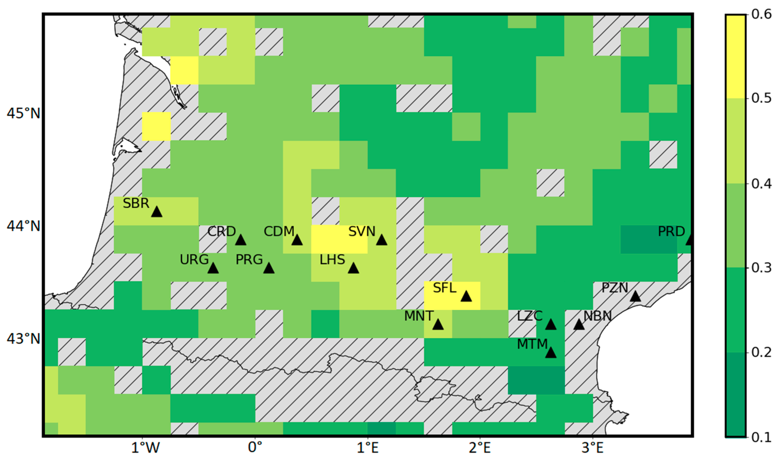
| Experiment (Time Period) | Assimilated Observations | Model Equivalent | Model Control Variables | ISBA Model Version | Atmospheric Forcing |
|---|---|---|---|---|---|
| OL (2007–2018) | n/a | n/a | n/a | Multi-layer soil, photosynthesis, interactive vegetation | ERA5 re-interpolated at 0.25° |
| EKF (2015–2018) | ASCAT σ040 | σ040 | LAI, WG2 to WG8 (0.01–1 m) | Multi-layer soil, photosynthesis, interactive vegetation | ERA5 re-interpolated at 0.25° |
| EKF_SWI_LAI (2015–2018) | ASCAT SWI-001 (rescaled) and PROBA-V LAI | WG2 (0.01–0.04 m), LAI | LAI, WG2 to WG8 (0.01–1 m) | Multi-layer soil, photosynthesis, interactive vegetation | ERA5 re-interpolated at 0.25° |
| Hyperparameter | Hidden Layers | Number of Neurons | Learning Rate | Epoch Number | Activation Function | Preprocessing of Predictors |
|---|---|---|---|---|---|---|
| Value | 1 | 40 | 0.001 | 250 | Relu | Z-score normalization |
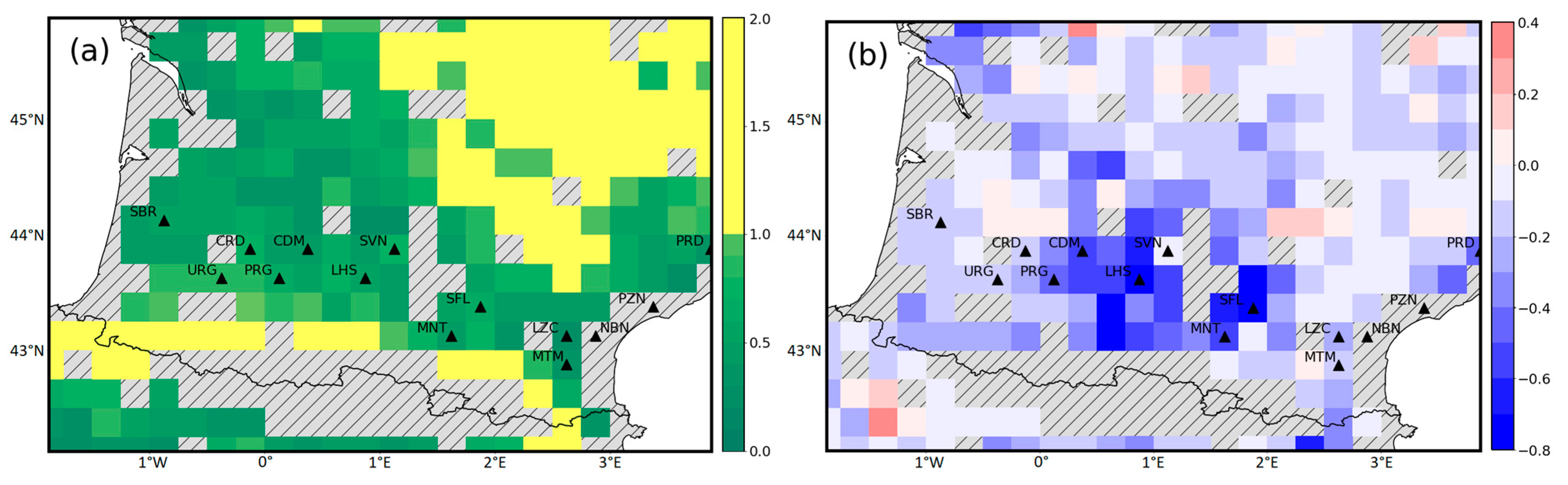
| Station Name | OL RMSD (dB) | EKF RSMD (dB) | OL R | EKF R | Number | RMSD Difference (dB) | R Difference |
|---|---|---|---|---|---|---|---|
| SBR | 0.45 | 0.37 | 0.76 | 0.86 | 1296 | −0.09 | 0.10 |
| URG | 0.37 | 0.34 | 0.74 | 0.79 | 1219 | −0.03 | 0.05 |
| CRD | 0.34 | 0.31 | 0.77 | 0.82 | 1220 | −0.03 | 0.05 |
| PRG | 0.70 | 0.34 | 0.55 | 0.82 | 1207 | −0.36 | 0.27 |
| CDM | 1.78 | 0.34 | 0.47 | 0.90 | 1209 | −1.44 | 0.43 |
| LHS | 1.62 | 0.33 | 0.53 | 0.93 | 1204 | −1.29 | 0.40 |
| SVN | 0.66 | 0.45 | 0.72 | 0.83 | 1228 | −0.22 | 0.11 |
| MNT | 0.97 | 0.35 | 0.39 | 0.81 | 1185 | −0.62 | 0.42 |
| SFL | 2.30 | 0.34 | 0.40 | 0.92 | 1227 | −1.96 | 0.52 |
| LZC | 0.54 | 0.25 | 0.30 | 0.69 | 1256 | −0.29 | 0.39 |
| MTM | 0.26 | 0.21 | 0.52 | 0.63 | 1191 | −0.05 | 0.11 |
| PRD | 0.98 | 0.31 | 0.04 | 0.58 | 1117 | −0.67 | 0.54 |
| Station Name | OL RMSD (m2m−2) | EKF RSMD (m2m−2) | OL R | EKF R | Number | RMSD Difference (m2m−2) | R Difference |
|---|---|---|---|---|---|---|---|
| SBR | 0.67 | 0.51 | 0.75 | 0.73 | 127 | −0.16 | −0.02 |
| URG | 0.97 | 0.83 | 0.67 | 0.71 | 120 | −0.14 | 0.05 |
| CRD | 0.85 | 0.73 | 0.76 | 0.81 | 121 | −0.12 | 0.06 |
| PRG | 1.11 | 0.69 | 0.65 | 0.70 | 119 | −0.42 | 0.05 |
| CDM | 0.96 | 0.41 | 0.74 | 0.78 | 118 | −0.55 | 0.04 |
| LHS | 1.30 | 0.53 | 0.65 | 0.82 | 114 | −0.77 | 0.17 |
| SVN | 0.84 | 0.76 | 0.66 | 0.44 | 114 | −0.08 | −0.23 |
| MNT | 0.99 | 0.48 | 0.77 | 0.85 | 115 | −0.51 | 0.08 |
| SFL | 1.41 | 0.65 | 0.70 | 0.60 | 119 | −0.76 | −0.10 |
| LZC | 0.51 | 0.29 | 0.85 | 0.88 | 119 | −0.22 | 0.03 |
| MTM | 0.49 | 0.37 | 0.80 | 0.84 | 114 | −0.12 | 0.04 |
| PRD | 0.84 | 0.38 | 0.75 | 0.78 | 110 | −0.46 | 0.02 |
Disclaimer/Publisher’s Note: The statements, opinions and data contained in all publications are solely those of the individual author(s) and contributor(s) and not of MDPI and/or the editor(s). MDPI and/or the editor(s) disclaim responsibility for any injury to people or property resulting from any ideas, methods, instructions or products referred to in the content. |
© 2023 by the authors. Licensee MDPI, Basel, Switzerland. This article is an open access article distributed under the terms and conditions of the Creative Commons Attribution (CC BY) license (https://creativecommons.org/licenses/by/4.0/).
Share and Cite
Corchia, T.; Bonan, B.; Rodríguez-Fernández, N.; Colas, G.; Calvet, J.-C. Assimilation of ASCAT Radar Backscatter Coefficients over Southwestern France. Remote Sens. 2023, 15, 4258. https://doi.org/10.3390/rs15174258
Corchia T, Bonan B, Rodríguez-Fernández N, Colas G, Calvet J-C. Assimilation of ASCAT Radar Backscatter Coefficients over Southwestern France. Remote Sensing. 2023; 15(17):4258. https://doi.org/10.3390/rs15174258
Chicago/Turabian StyleCorchia, Timothée, Bertrand Bonan, Nemesio Rodríguez-Fernández, Gabriel Colas, and Jean-Christophe Calvet. 2023. "Assimilation of ASCAT Radar Backscatter Coefficients over Southwestern France" Remote Sensing 15, no. 17: 4258. https://doi.org/10.3390/rs15174258
APA StyleCorchia, T., Bonan, B., Rodríguez-Fernández, N., Colas, G., & Calvet, J.-C. (2023). Assimilation of ASCAT Radar Backscatter Coefficients over Southwestern France. Remote Sensing, 15(17), 4258. https://doi.org/10.3390/rs15174258