1. Introduction
In forests, wood productivity is of interest in commercial forestry to determine economic value and to support the planning of silvicultural treatments. Mapping of forest productivity and age can also be useful in monitoring and modeling forest biomass (carbon stock) and changes in this over time. Forest productivity can be expressed in terms of site index (SI), a variable expressing the expected height of dominant trees at a reference age, given the local conditions. In addition to being a useful tool in economic assessments, forecasting, and planning in the commercial management of forests, large-scale mapping of SI can be used to quantify the effects of environmental changes, such as mean temperature changes or droughts, on the productivity of forests [
1]. Such mappings can be used to make predictions about the geographically distinct consequences of climate change.
SI can be determined based on climatic and field conditions such as precipitation, temperature, and classification of soil strata, which is useful when no trees are present on the site. Another way to estimate SI uses age and dominant- or top-height measurements and is generally favored over the previous method due to its practicality, low cost, and higher accuracy. It requires the location to have an established even-aged forest and relies on a strong correlation between volume growth and height growth [
2]. The definitions of top height vary, where some are based on the mean height of dominant trees, and others on the maximum tree height, or the mean height of a certain percentage of the highest trees in an area. In Sweden, the SI estimated from top height describes the site productivity for the dominant species in terms of the achievable height in meters of the largest diameter trees at a specific reference age (
ASI). The top height is defined as the mean height of the 100 trees with the largest diameter at breast height per hectare. This definition of top height is sometimes called H100, and is meant to represent the upper height of tree crowns in the forest. Top height has successfully been estimated using different remote sensors. Examples include estimating top height with the maximum airborne laser scanning (ALS) canopy model height in a 10 m × 10 m window, or the maximum height in 500 m
2 plots of an aerial stereo-image-based canopy height model (CHM) [
3,
4].
While SI is not the most commonly estimated forest variable, it has been successfully predicted, often together with the related variable stand age, using a few different approaches, sensors, and sensor combinations. Commonly stand or tree heights are estimated by some remote sensing techniques and compared to known height–age curves to determine SI and age [
5,
6,
7,
8,
9,
10,
11]. Véga and Onge [
5] used CHMs based on historical aerial photographs and ALS from four time points spanning a period of 58 years to predict SI and age. Their models were estimated by minimizing mean absolute residuals to age-height curves, where the heights were extracted from CHMs calibrated with individual tree growth reconstruction. This method required counting tree rings on the cross-sections of felled trees to derive correction equations between tree heights from manual CMH interpretation and the field reconstructed heights. The procedure resulted in 2.4 m RMSE for SI and seven years RMSE for age predictions on 400 m
2 plots. Kandare et al. [
6] used an individual tree crown (ITC) approach for predicting SI in boreal forests using airborne laser scanning (ALS) and hyperspectral data. They estimated the age, height, and diameter at breast height of the dominant trees from ALS and hyperspectral metrics. These were then used in age-height curves to predict SI. When predicting both SI and age, the method by Kandare et al. achieved RMSEs of 4.3 m and 34 years, respectively. When the age from field data was used in the prediction, the RMSE of SI predictions dropped to 1.18 m [
6]. Solberg et al. used age-independent equations of top height growth and single tree ALS data to predict SI by matching single dominant trees in repeated ALS measurements six years apart [
7]. They estimated SI values very close to field-based values for individual sample trees (bias 0.27 m, RMSE about 2.8 m, as interpreted from a figure). Penner et al. [
8] used two successive ALS collections, acquired 13 years apart, to estimate SI with an RMSE of 2.5 m and a bias of 0.3 m on 400 m
2 field plots.
Many of the reported results are good but require access to long time series, as in the case of [
5], rely on relatively costly ALS data, usually from several years, or on local calibration of remote sensing data or predicted attributes. Synthetic Aperture Radar (SAR) provides a cost-efficient alternative to ALS and aerial photography that is independent of sunlight and relatively unhindered by clouds and precipitation, thereby providing reliable year-round coverage of large parts of the world from different spaceborne systems. These operate in different parts of the microwave spectrum, called bands, corresponding to different wavelengths. Shorter wavelengths, such as the X and C bands, have significant contributions from the top part of the canopy and are, therefore, well suited for canopy height estimation using single-pass SAR interferometry (InSAR). Sentinel-1, a C band SAR system that provides open access data over large parts of the world, does, however, not have single-pass capability. TanDEM-X (TerraSAR-X add-on for Digital Elevation Measurement) is a two-satellite constellation that captures single-pass interferometric InSAR images at X-band (wavelength 3.1 cm). It provides data over a large part of the world and has proven itself valuable in forest variable retrieval [
12,
13]. Several studies have used TanDEM-X for the retrieval of forest variables [
3,
14,
15,
16,
17]. Many of these have estimated forest heights from TanDEM-X data [
3,
14,
17,
18,
19,
20,
21], and a few have investigated height development due to deforestation, silvicultural treatments, or growth [
22,
23,
24], or used phase height development to estimate biomass and volume changes [
25,
26,
27].
The use of TanDEM-X data for SI prediction has so far been limited to Persson and Fransson [
9], Wallerman et al. [
10], and Persson and Fransson [
11]. In these studies, simple linear models relating TanDEM-X phase heights to ALS percentiles or Lorey’s heights (i.e., basal area weighted mean heights) from field data were used as calibration. Wallerman et al. [
10] estimated SI when the age was provided, with an RMSE of 18.6% (corresponding to around 6–7 m, as interpreted from a figure) on 314 m
2 plots. They used TanDEM-X image pairs from three growth seasons calibrated using ALS data. Persson and Fransson [
11] used four TanDEM-X acquisitions covering three growth seasons, calibrated using ALS data or Lorey’s height from field data. They predicted SI with 4.4 m RMSE and age with 17.8 years RMSE on 0.5 ha plots. The need for calibration, however, hampers the scalability of the methods, as it relies on local high-resolution ALS data or field data. Furthermore, the usefulness of calibration data decreases with the time between data collection and the TanDEM-X acquisition date due to forest growth and other changes. Because of this, longer time series may often need calibration data from multiple time points.
In this study, we wanted to use a longer and denser time series of TanDEM-X acquisitions than in the previous studies and simultaneously avoid the use of calibration of the TanDEM-based heights via ancillary remote sensing or field data. Additionally, all remote sensing studies predicting SI that we are aware of use only plots, which appear to be unaffected by silvicultural treatments during the observation period. This study included plots subject to different silvicultural treatments during the study period to assess the potential effects on the predictions.
The remainder of the paper is structured as follows:
Section 2 starts with a description of the test site and field data, after which the TanDEM-X data and its processing into TanDEM-X-based top heights are detailed. After this, established height development curves (HDC) and how they are used to calculate SI from field-measured top height and age are described. This is followed by a description of the method by which the SI and age are predicted by fitting an HDC to the time series of TanDEM-X-based top heights and how the results were evaluated.
Section 3 presents the results of SI and age predictions.
Section 4 contains a discussion of the results, and finally,
Section 5 concludes the paper.
2. Materials and Methods
2.1. Test Site and Field Data
The study was conducted in Remningstorp, a forest test site located in southern Sweden (Lat. 58°30′N, Long. 13°40′E), consisting of about 1200 ha of commercially managed hemi-boreal forest. About two-thirds of the forest grows on till, a mixture of glacial debris, with, except in old spruce stands, a field layer of herbs, blueberry (Vaccinium myrtillus L.), and narrow-leaf grass (e.g., Deschampsia flexuosa (L.) Trin.). The main tree species are Norway spruce (Picea abies (L.) H. Karst.), Scots pine (Pinus sylvestris L.), and birch (Betula spp.). The rest of the forest grows on peatland, dominated by Scots pine. The landscape is mainly flat, with mild slopes, located 120 m to 145 m above sea level.
SI was determined for 91 circular field plots with a 10 m radius in a survey carried out in the fall of 2021. The age and height of two dominant trees per plot were measured, and the dominant species recorded. SI was calculated from the mean age and height for each plot. Using forest treatment records and inspection of biannual aerial orthophotos, the plots were classified into 2 clear-cut plots, 45 thinned plots, 7 pre-commercially thinned plots, and 26 untreated plots. Among the 91 plots, 11 plots were not covered by the available treatment records nor determined clear-cut in the inspection of orthophotos and, therefore, referred to as “undocumented”. While clear-cuts were evident in the available orthophotos, thinnings were difficult to detect, and it is likely that a significant portion of these undocumented plots were, in fact, thinned or pre-commercially thinned.
Table 1. shows the mean and range of SI and the field-measured variables for each treatment group.
SI values based on a previous field survey in 2014 were also available for 51 of the plots. Since the inherent productive potential of a specific site is not expected to change significantly in seven years, this dataset provided a means to characterize the uncertainty in the reference data. For these 51 plots, the variation in terms of Root Mean Square Deviation (RMSD) and bias, calculated according to Equations (1) and (2), between the 2021 and 2014 surveys of SI was 3.3 m and 2.0 m, respectively.
2.2. SAR Data
Thirty TanDEM-X scenes were acquired in a bi-static configuration over Remningstorp between 11 August 2013 and 24 September 2018. The scenes were acquired in strip-map mode and included a vertical transmit/receive (VV) polarization, acquired either as a single polarization or as a single channel from a dual-polarization scene. The bandwidths were 100 MHz or 150 MHz, respectively. A single polarization was chosen to avoid polarization-dependent systematic differences in phase heights, and the VV polarization specifically was chosen because it provided the best temporal coverage of the time period under study. Furthermore, using meteorological records, only acquisitions from dates preceded by a three-day average temperature of above 5 °C were included since freezing temperatures severely affect the observed radar phase heights from vegetation. The height of ambiguity, HoA, ranged between 43 m and 100 m, but most scenes were acquired with a HoA between 50 m and 65 m. The incidence angles ranged from 19° to 40°.
The data were delivered in the Coregistered Single look Slant range Complex (CoSSC) format. A complex interferogram was computed with 5 × 5 spatial averaging in range and azimuth. The interferogram was flattened with respect to earth curvature, and Goldstein filtered [
28]. The flattened phase was unwrapped and converted to phase height by scaling with the wavenumber, and the interferometric coherence was estimated from the flattened interferogram using a coherence window of 3 × 3 pixels. Finally, the scenes were interpolated to a ground resolution of 10 m × 10 m. The estimated coherence was corrected for decreasing signal-to-noise ratio [
3,
15,
17].
The radar signal penetrates significantly into the canopy, and for boreal coniferous forests, this leads to a negative elevation bias of the canopy heights that can sometimes be as large as 10–20 m [
3]. In [
29], a correction of this bias was proposed, which has successfully been evaluated on TanDEM-X data over temperate and hemi-boreal forests [
24,
30]. According to [
29], the canopy height bias is given by
where γ is the volume coherence, and
HoA is the height of ambiguity. The InSAR phase center heights in the time series were corrected for elevation bias by calculating
Δℎ on pixel level and correcting the height values to produce InSAR-based canopy heights. A thorough derivation of (3) is given in [
29]. As the bias correction assumes penetration into an infinite volume, it is not theoretically valid when the signal has significant ground contributions, and as a rule of thumb, the canopy height should be at least twice the bias correction. The correction was applied to all plots, although some field plots with low canopy heights or sparse forests could potentially violate this criterion. The ground contributions to the pixels with the highest phase heights on each plot are generally assumed to be small, and as described in
Section 2.3, only the highest InSAR canopy heights on each plot influence the estimated top height in the method applied. However, ground contributions are likely dominant in clear-cut plots after treatment, but these were nevertheless corrected using Equation (3).
Each acquisition was assigned an integer representing its growth period based on the date of acquisition. A growth period was defined to start on 15 June, approximating the halfway point of the actual growth period, and last for one year. The earliest acquisition date was assigned to growth period 0, and the latest acquisitions were assigned to growth period 5.
2.3. Top Height Estimation
For each date, the corrected phase height values of pixels covered or intersected by a polygon defining the field plot region were extracted. In order to estimate the top height from these pixels, the 90th height percentile was calculated for each plot and date. Different percentiles were investigated, and generally, the higher percentiles correlated better with field-measured top heights. The 90th height percentile will hereafter be referred to simply as TanDEM-X top height.
2.4. Site Index
Established HDCs for common Swedish tree species, as developed in [
31,
32] and summarized in [
33], describe the expected top height
H2 at stand age
A2, given a measured top height
H1 at stand age
A1:
where
β and
b2 are previously determined tree species-specific fixed parameters, and
ASI is the reference age. Equation (4) is commonly used to calculate SI given field measurements of top height and age, as was done with the field data in this study. By setting
A2 to the preferred SI reference age and
H1 and
A1 to the measured height and age,
H2 equals the SI. The HDCs were developed from multiple measurements on sets of field plots in even-aged forests, the predominant forest type in Sweden, and are therefore valid in such forests.
If
H1 is set to a specific SI value instead of a measured height and
A1 is set to the corresponding reference age,
H2 gives the expected top height at any age
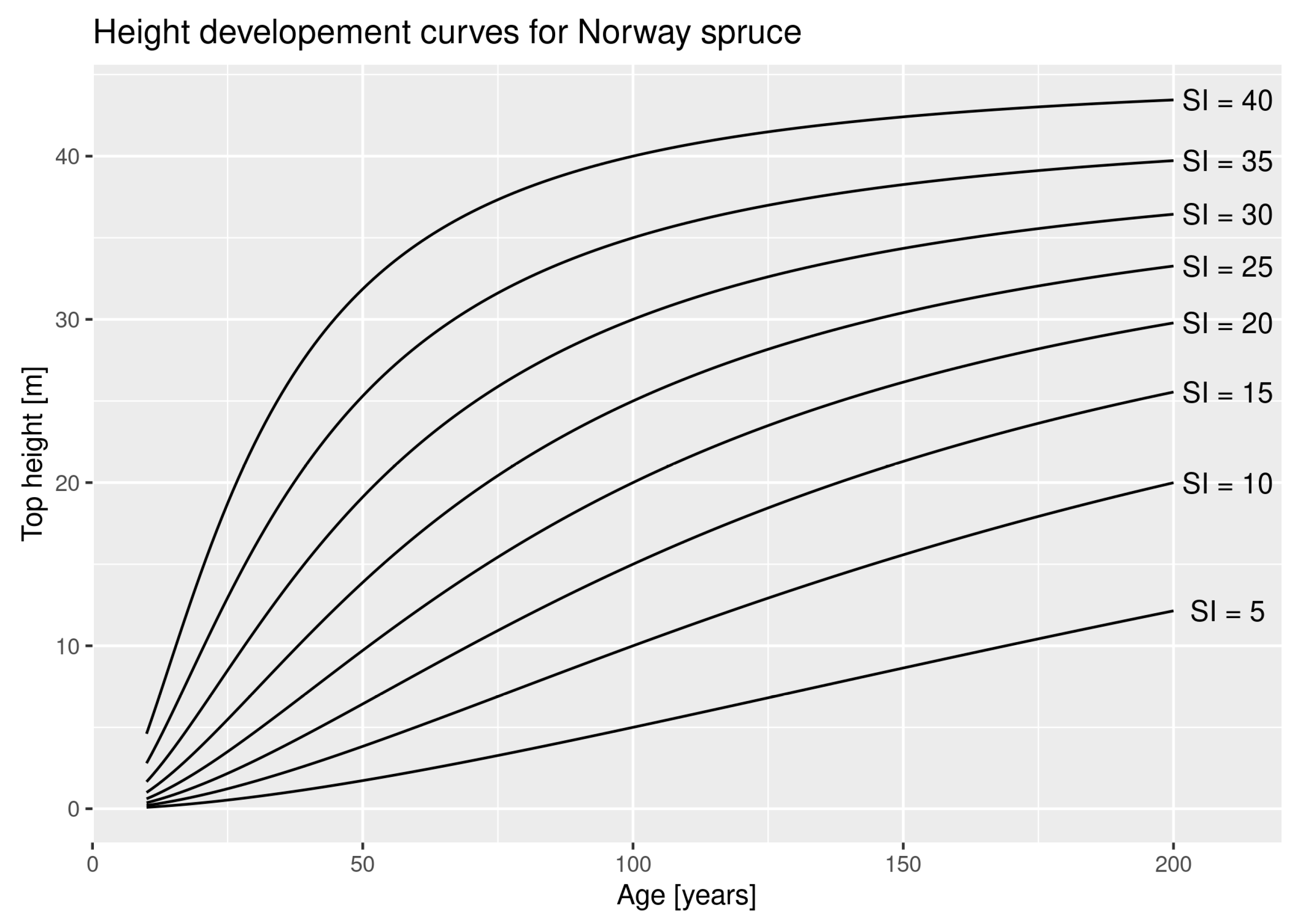
A2. For illustration, the resulting HDCs of Norway spruce for a few values of SI are shown in
Figure 1.
2.5. Site Index Estimation
Setting
H1 and
A1 in Equation (4) to SI and the corresponding reference age, respectively, and substituting
A0 +
GP (growth period) for
A1, allows us to express TanDEM-X top height
H as a function of SI and
GP, explicitly
SI and
A0 were determined by applying a weighted non-linear least squares regression of Equation (7) to the time series of TanDEM-X top heights, leaving initial age (age at the time of the first TanDEM-X measurement,
A0) and/or SI as parameters. The function was fit to each field plot using dominant species information from the field data to select the correct fixed parameters, and two different prediction cases were applied; (a) estimates of both SI and
A0 for each plot, and (b) estimates of only SI, assuming that the initial age is known. In case (b),
A0 in the fitting was supplied from the field data.
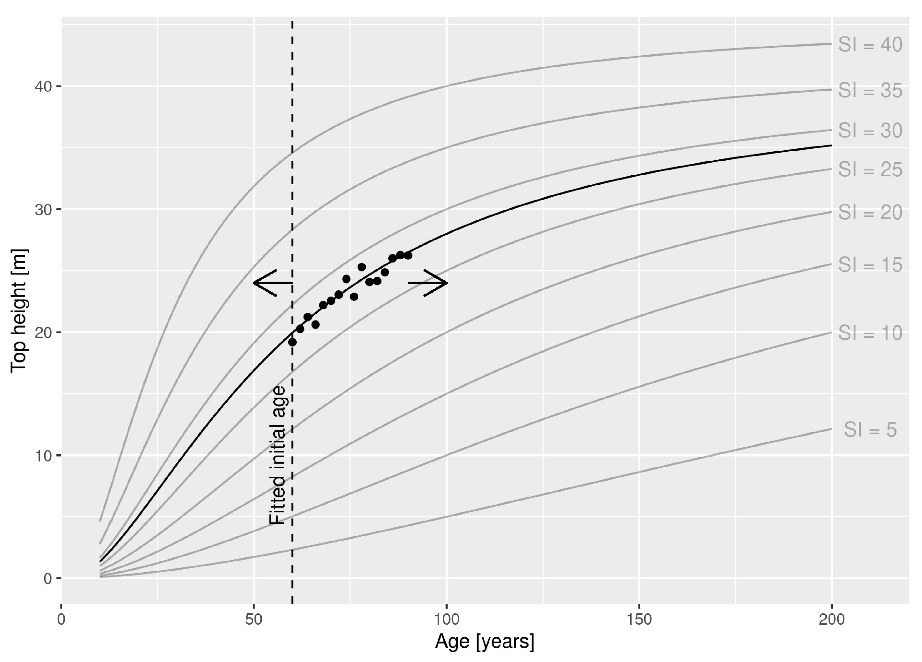
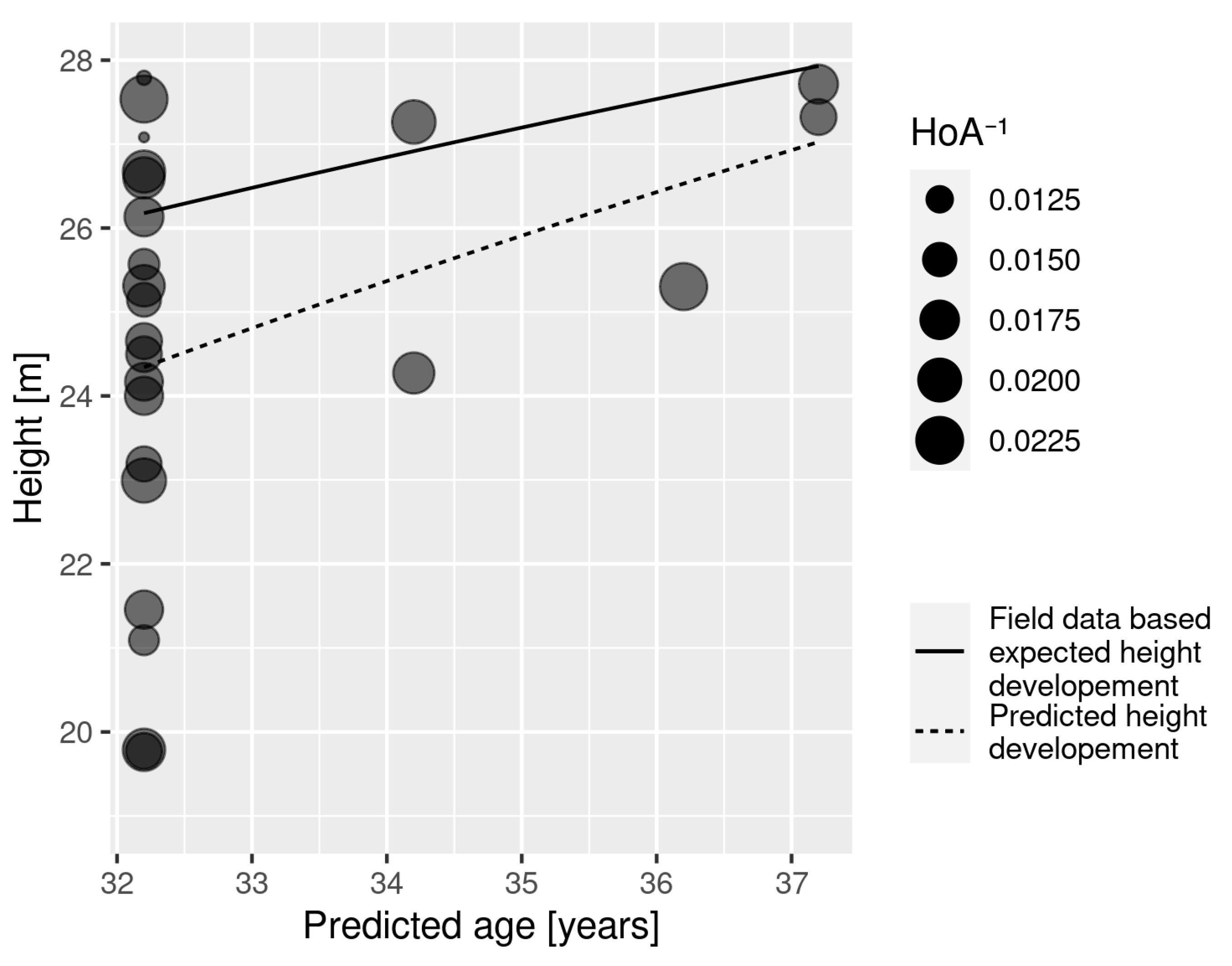
Figure 2 illustrates prediction case (a). In this figure, the process of fitting
A0, can be considered as a translation in time of the time series of TanDEM-X top heights to find the optimal fit, while the fitting of SI corresponds to the choice of optimal curve out of the family defined by Equation (7).
The least squares regression was performed using the
nls function from the
stats package of the open-source
R programming language [
34]. By using the
port algorithm, the solver utilized an implementation of the
nl2sol algorithm [
35]. The SI and
A0 (in prediction case (a)) were initialized to 25 and 75 and constrained to the intervals [4, 60] and [4, 200], respectively. This algorithm was chosen because of the possibility of setting bounds for the parameters. Otherwise, the algorithm tended to diverge or produce implausible parameter values for plots where TanDEM-X phase heights decreased over time. In case the fitting did not converge, it was restarted and initialized using the parameter values obtained in the non-converging fit.
The uncertainty of the InSAR phase height is, up to a critical value, roughly inversely proportional to the interferometric baseline [
36] and hence proportional to
HoA. Because of this, scenes with a baseline below, or equally an
HoA above, some threshold value are often omitted in pursuit of high precision. In order to account for the
HoA-related uncertainty without sacrificing temporal resolution, each observation was weighted in the fitting procedure with the reciprocal of
HoA.
The SI and
A0 predicted by parameter estimation were visually inspected via plots of the fitted HDC alongside the TanDEM-X top heights and the HDC expected from the field-data-based SI and age. The quality of predictions of
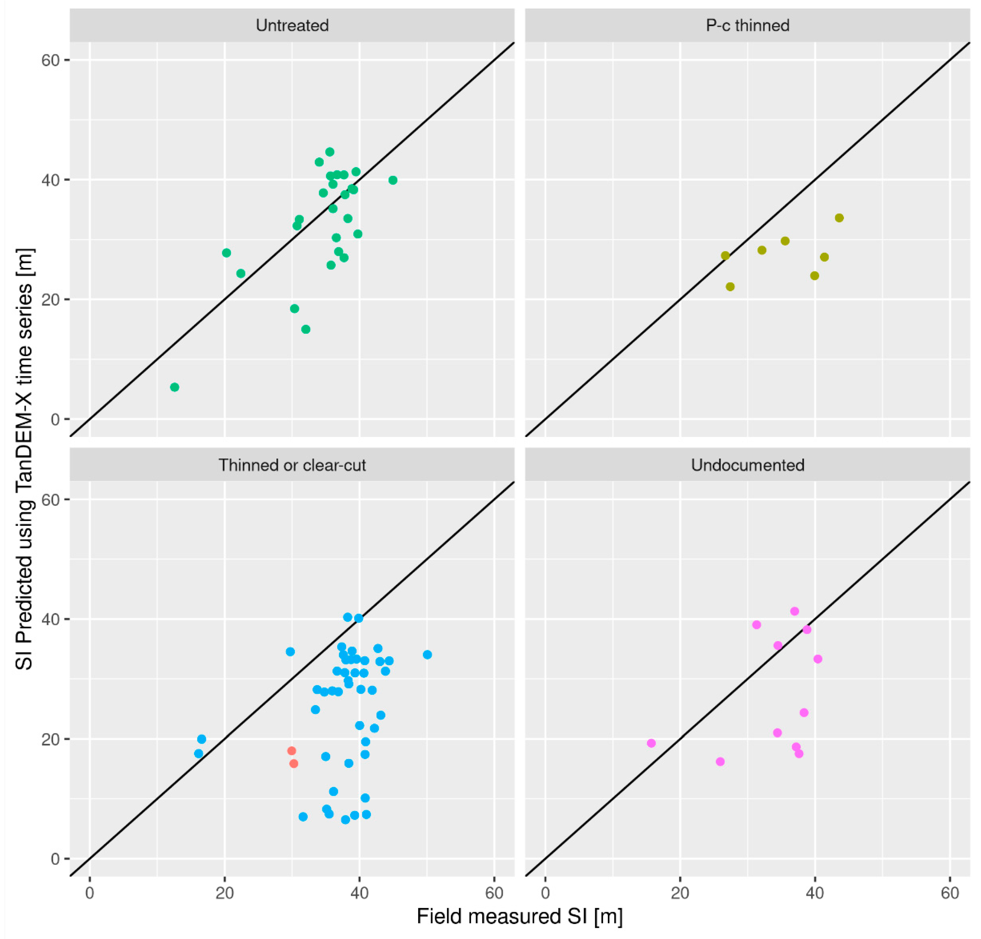
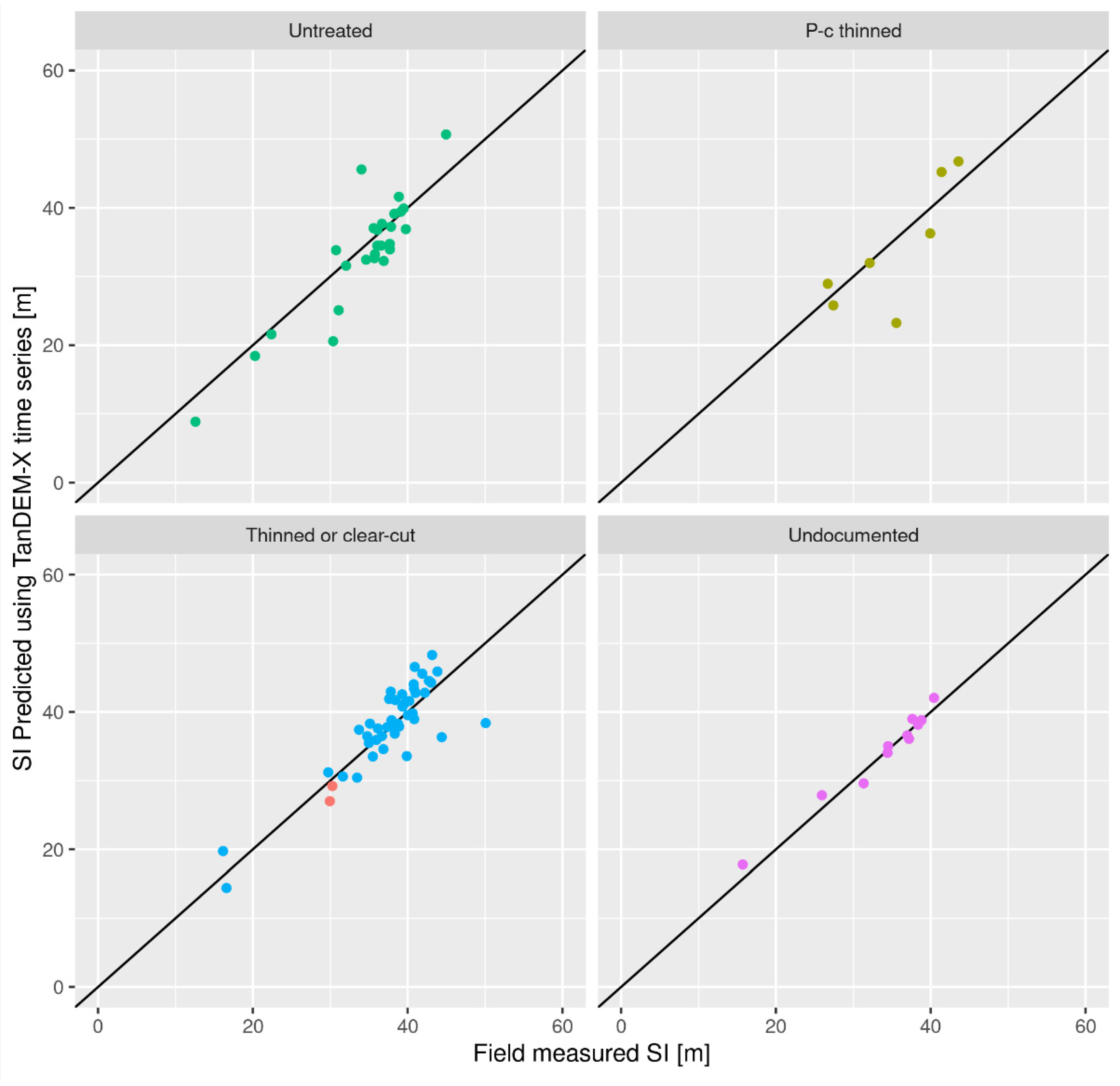
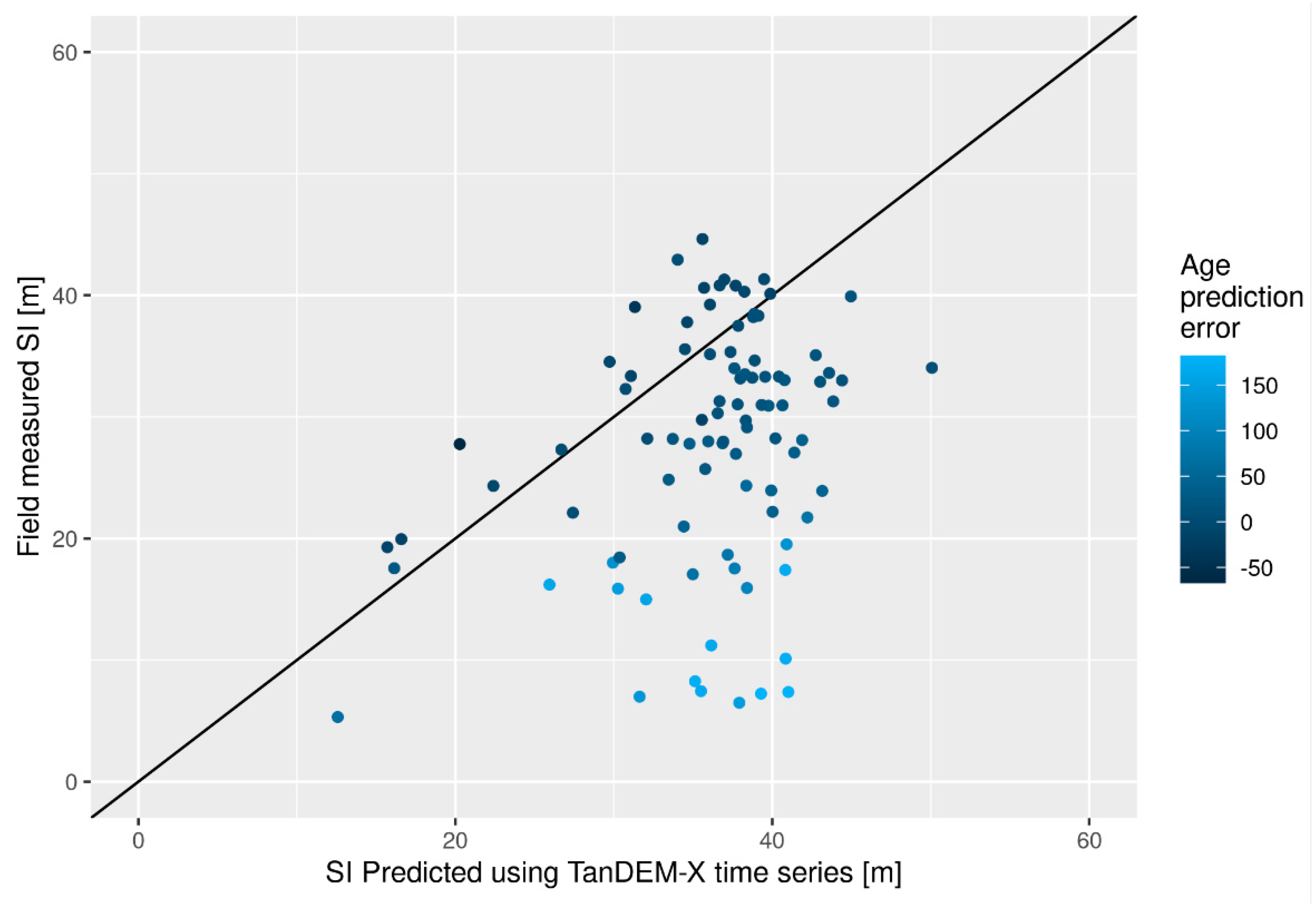
A0 and SI were evaluated by comparisons with the corresponding field-data-based values, and prediction results were further visually evaluated through plots to investigate possible correlations between prediction errors and SI, stand age, species, or treatment groups. The Root Mean Square Error (RMSE) and bias were calculated for each treatment group
k as
where
is the
ith prediction,
the corresponding field data value, and
nk is the number of field plots in group
k. Additionally, the coefficient of determination between predictions and reference values was calculated.
4. Discussion
The TanDEM-X top height, i.e., the 90th height percentile of bias-corrected phase heights, captured the canopy top height reasonably well. This was evidenced by (1) the relatively small and statistically insignificant prediction biases on untreated plots in case (a), when predicting both SI and age, and (2) the very low RMSE and bias of the predictions of SI in case (b), when age was provided from field data.
The RMSE of 4.0 m for prediction case (b) is significantly lower than the RMSE of 6–7 m in [
10], which used ALS-calibrated TanDEM-X heights and similarly predicted only SI on 10 m radius plots. In [
10], the prediction of both SI and age using TanDEM-X data (corresponding to case (a) in this paper) was unsuccessful due to divergent solutions.
The RMSE for untreated plots in prediction case (a), 6.9 m, is larger than some previous studies [
5,
7,
8,
9,
11], but they cannot be directly compared, as they differ in SI reference ages and/or the area of evaluation units. For example, this study used 10 m radius plots, while in [
11], reporting 4.4 m and 17.8-year RMSEs, the plots were 16 times larger. In other studies, such as [
5] (2.4 m RMSE) and [
7] (about 2.8 m RMSE), the reported SI predictions differed in species and the reference age (50 years in [
5], 40 years in [
7]) at which the SI height is defined, due to local functions and practices.
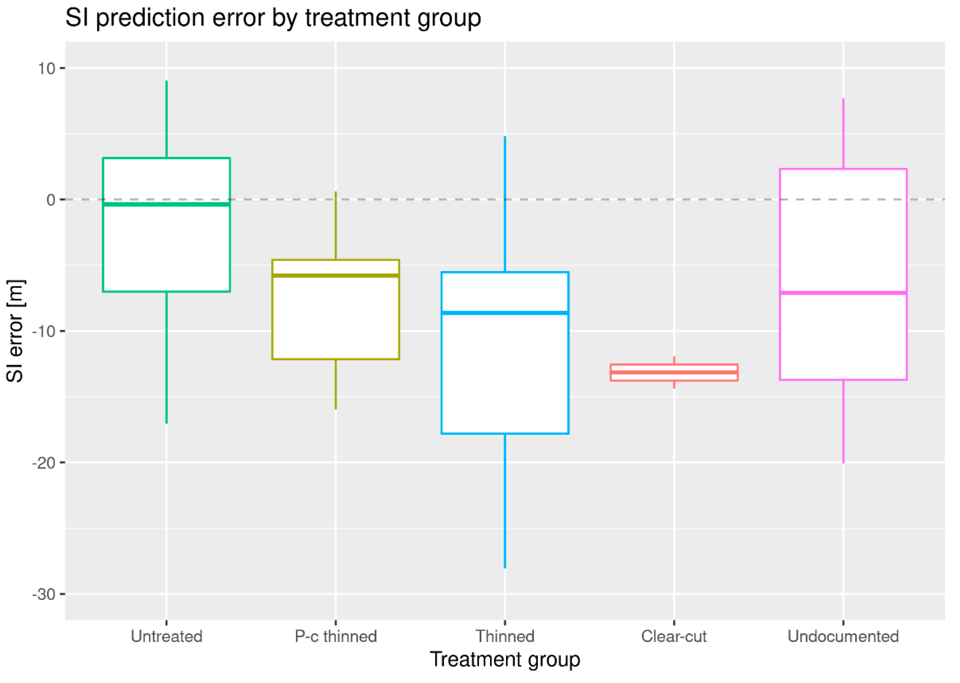
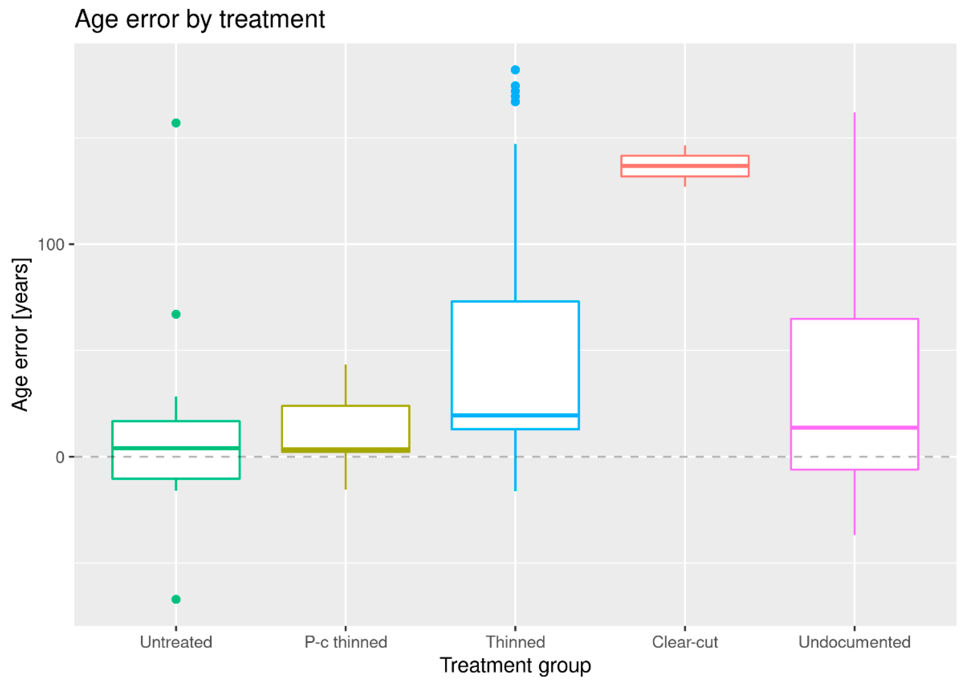
Silvicultural treatments, from pre-commercial thinning to clear-cutting, lead to underestimation of the slope of the HDC, which in turn leads to underestimation of SI and overestimation of age. This tendency increased with the intensity of treatment.
We did not observe systematically larger prediction errors for mature stands, as observed in, for example, [
5], where predictions based on measurement periods capturing later stand development stages with lower height growth rates produced more uncertain estimates of both SI and age. As the growth rate decreases with age, the importance of absolute height estimates increases (
Figure 2). The absence of increased prediction uncertainty for older untreated plots further indicates that the absolute top height is estimated well by the TanDEM-X top height.
Some of the uncertainty in predictions is explained by edge effects. From inspection of orthophotos, we found that plots with large deviations between predictions and reference values were often located close to, or even across, stand boundaries or roads since the plot locations in the field surveys were distributed in a systematic grid. During the analyses, it was found that for such plots, the measured phase heights could be drastically different depending on look direction, which caused us to use only acquisitions from a descending orbit. This maximized the duration and resolution of the time series. Removal of such edge plots would likely have led to lower RMSEs in the predictions, but they were nevertheless kept in order to better reflect realistic results with a minimum amount of manual intervention. Because of this, it is also reasonable to expect higher precision for larger prediction units, where boundary effects have a smaller impact on the prediction or can be dealt with, for example, by using buffer zones.
Given the small prediction biases observed for untreated plots in case (a) and the apparent overall precision of top height estimates, we expect even longer time series to increase the quality of predictions of both SI and age significantly from the results for prediction case (a) in untreated plots. Longer time series may also mitigate the underestimation of slope resulting from treatments if the influence of such treatments on the TanDEM-X top height is transient in nature. Future studies should investigate the inclusion of multiple polarizations as a way to further increase usable observations.
Further, the prediction of SI and age via weighted non-linear regression readily accommodates the inclusion of other height data sources since top heights based on any source could simply be added to the time series and weighted according to the uncertainty of the source. Alternatively, since the SI prediction quality was shown to be much better assuming known age, the method could also be combined with other data sources by supplying age from field data or predictions from photogrammetric time series, as in [
37]. In this study, the dominant species was assumed to be known, but in a practical application, the dominant species could also be predicted based on other data sources.
It should be noted that although the method proposed does not use any ancillary field data or remote sensing data such as ALS for calibration of the TanDEM-X data, it does require an accurate DTM in order to obtain reliable canopy heights from phase heights. This requirement is fulfilled in a rapidly increasing part of the world. Additionally, the HDCs used are developed using data from even-aged stands, and their applicability in other types of forest should be further investigated.
As the method presented does not rely on local calibration and easily accommodates and benefits from additional TanDEM-X scenes that extend or increase the temporal resolution of the prediction period, it is suited for producing wall-to-wall estimates over large areas of forest.
5. Conclusions
SI, the expected top height at some reference age, and stand age are important variables in forest management and forecasting. This study presented and evaluated a method of predicting SI and age using only time series of TanDEM-X data and a DTM.
The method consists of fitting established HDC to the time series, using the 90th height percentile of canopy penetration corrected phase heights as a surrogate for forest top heights. Predicted SI and age were retrieved as parameter values minimizing the squared top height residuals.
SI and age could be unbiasedly predicted for untreated plots, and the RMSE of predictions is likely to decrease with the length and temporal resolution of the time series available. When the stand age was known, the SI was predicted with an RMSE comparable to that of field-based measurements.
The results for treated plots indicate that the RMSE and bias of predictions increase with the intensity of silvicultural treatments, with a larger relative decrease in stem volume on average leading to a larger underestimation of SI and an overestimation of stand age and a higher RMSE for both variables.
In general, the results demonstrate viability for large-scale wall-to-wall mapping of SI using time series of TanDEM-X data without the need for ancillary data for height calibration. Further studies should investigate the use of multiple polarizations and both orbit directions to increase the length and temporal density of useful time series in an effort to further increase the obtained prediction quality.
