Article

Comparison of Machine Learning Models to Predict Lake Area in an Arid Area

1
Center for Agricultural Water Research in China, China Agricultural University, Beijing 100083, China
2
Ordos City River and Lake Protection Centre, Ordos 017010, China
3
Ordos Water and Drought Disaster Prevention Technology Centre, Ordos 017010, China
*
Author to whom correspondence should be addressed.
Remote Sens. 2023, 15(17), 4153; https://doi.org/10.3390/rs15174153
Submission received: 26 June 2023 / Revised: 10 August 2023 / Accepted: 14 August 2023 / Published: 24 August 2023
(This article belongs to the Special Issue Advances in Remote Sensing of Ecohydrology)

Abstract

:
Machine learning (ML)-based models are popular for complex physical system simulation and prediction. Lake is the important indicator in arid and semi-arid areas, and to achieve the proper management of the water resources in a lake basin, it is crucial to estimate and predict the lake dynamics, based on hydro-meteorological variations and anthropogenic disturbances. This task is particularly challenging in arid and semi-arid regions, where water scarcity poses a significant threat to human life. In this study, a typical arid area of China was selected as the study area, and the performances of eight widely used ML models (i.e., Bayesian Ridge (BR), K-Nearest Neighbor (KNN), Gradient Boosting Decision Tree (GBDT), Extra Trees (ET), Random Forest (RF), Adaptive Boosting (AB), Bootstrap aggregating (Bagging), eXtreme Gradient Boosting (XGB)) were evaluated in predicting lake area. Monthly lake area was determined by meteorological (precipitation, air temperature, Standardised Precipitation Evapotranspiration Index (SPEI)) and anthropogenic factors (ETc, NDVI, LUCC). Lake area determined by Landsat satellite image classification for 2000–2020 was analysed side-by-side with the Standardised Precipitation Evapotranspiration Index (SPEI) on 9 and 12-month time scales. With the evaluation of six input variables and eight ML algorithms, it was found that the RF models performed best when using the SPEI-9 index, with R2 = 0.88, RMSE = 1.37, LCCC = 0.95, and PRD = 1331.4 for the test samples. Furthermore, the performance of the ML model constructed with the 9-month time scale SPEI (SPEI-9) as an input variable (MLSPEI-9) depended on seasonal variations, with the average relative errors of up to 0.62 in spring and a minimum of 0.12 in summer. Overall, this study provides valuable insights into the effectiveness of different ML models for predicting lake area by demonstrating that the right inputs can lead to a remarkable increase in performance of up to 13.89%. These findings have important implications for future research on lake area prediction in arid zones and demonstrate the power of ML models in advancing scientific understanding of complex natural systems.

1. Introduction

In arid and semi-arid areas, lakes are important freshwater resources to maintain the local ecology [1]. Furthermore, lake area is an important indicator of arid accident and local water resources. However, lakes have changed significantly over the past decades owing to the synergistic effects of climate change and human activities [2,3,4]. Lakes are the most specific factors in surface water bodies and global climate change, and land-use and land-cover changes are leading to profound changes in lakes. Arid and semi-arid regions are particularly susceptible to hydrological changes, making lakes in these areas especially sensitive and vulnerable to human activities, climate change, and their interplay [5,6]. Intensive irrigation practices, particularly in arid regions, have resulted in negative environmental impacts including drought, desertification, dust storms, and soil salinisation [7].
Therefore, monitoring vulnerable lakes in arid and semi-arid regions is crucial for effective government decision making. Lakes are very sensitive to climatic and weather conditions, posing considerable challenges to the study of their dynamic nature. Traditional monitoring methods, which are time-consuming, labour-intensive, and often unable to accurately measure the actual lake area, result in insufficient surveying and monitoring of lakes, particularly in remote regions like the Mu Us Sandy Land.
Fortunately, satellite-based observations offer a promising solution to this dilemma [8]. By leveraging satellite image analysis, we gain a valuable tool to estimate changes in the physical and biological properties of aquatic and terrestrial ecosystems. Studies based on satellite imagery have determined the dynamics, variability [9,10], morphology [11], and surface area of lakes [2,12]. A low-to-medium resolution of 30 m is preferred for longer time series, given the spatial and temporal resolution of satellite sensors. The Google Earth Engine (GEE) platform, with its remarkable advantages in handling vast remote sensing data and providing abundant computing resources and storage space, has been widely used in various research fields in recent years.
Because of the influence of water cycle processes, lake area changes seasonally and reaches its maximum during the rainy season. Many models have been used to predict changes in lake area. For example, Guo et al. (2022) proposed a time series model based on the ARIMA (autoregressive integrated moving average) to predict the area of Qinghai Lake for the next three years [13]. Harris et al. (1989) used remote sensing data to conduct a remote sensing survey of the watershed area of the Northern Ireland Lake, and the relationship between watershed area change and water level was also discussed in detail [14]. Zeng et al. (2008) found that lake shrinkage was linked to urban construction, road traffic planning, policy orientation, and other factors in the area [15]. In addition to the use of 3S techniques for estimating the lake areas reviewed above, studies using data-driven models for lake area prediction are increasingly being developed. In water resources, phenomena are governed by the laws of physics and involve relationships with amorphous boundaries and complex underlying variables [16]. Most of the processes are studied through simulations using physically based mathematical models running on computers. Running such physics-based models for large real-world systems is computationally intensive and difficult to generalise for a number of reasons. The primary data sources for water resources modelling come from observations of relationships simulated in terrestrial, spatial, and water bodies, along with surveys, laboratory experiments, and multi-year systematic studies. The data collected include a large number of potential variables from multiple sources, at multiple resolutions in space and time, with varying degrees of skewness and uncertainty. To overcome these challenges, several research communities, including hydroinformatics, climate informatics, the American Geophysical Union, and earth and space science informatics, have been focusing on the application of machine learning techniques that have shown promising performance in hydrologic and water resource applications [17]. Simple data-driven models outperform theory-driven models in terms of prediction accuracy in many hydrological applications [18].
With the continuous development of computer science and Deep Learning Algorithms (DLAs), data-driven hydrologic modelling appears to be a reliable alternative to traditional process-based hydrologic models [19].
In the past decades, data-driven models have been used as powerful tools for general-purpose computational modelling; related applications have rapidly developed in different areas of hydrology, and their performance has been widely recognised [20]. For example, attempts to predict lake area using supervised learning based on available information are increasing and have accelerated significantly since 2019. A wide range of ML algorithms providing supervised, semi-supervised, and unsupervised models enable the prediction of geographic elements and provide a fresh perspective on the estimation of the area of water bodies such as lakes. In view of this, based on existing studies, integrated learning algorithms have been introduced to combine time series for multi-factor analysis affecting lake area change, revealing the correlation and importance of lake area change from multiple scales such as climate and drought conditions in the study area and laying a solid data foundation for research on spatial pattern evolution and driving mechanisms. Table 1 reports the main references summarising the characteristics of previous studies on regression prediction using ML algorithms [21,22,23,24,25,26,27,28]. In this study, we tested ML methods for predicting lake area, with a particular focus on RF, ET, and GDBT, and, considering the choice of predictors and the characteristics of ML algorithms, investigated how we can improve the performance of ML models. For example, does the choice of different time scales of the input variables also contribute to better results? This study aims to fill the research gap by providing a systematic analysis of the choice of predictors and the performance of different ML algorithms.

2. Materials and Methods

2.1. Study Area

The Mu Us Sandy Land is located in the northern part of the Loess Plateau and the southern part of the Ordos Plateau, specifically at the junction of Inner Mongolia, Shanxi provinces, and Ningxia Hui Autonomous Region. This region represents a transitional zone between the Loess Plateau and the Ordos Plateau, making it one of the four major sandy areas in China. In this study, the Mu Us Sandy Land (107°29′~109°56′E, 37°37′~39°33′N, 27,800 km2) in Ordos City, Inner Mongolia, was selected for the study, and the administrative areas were mainly distributed in five banners and counties, namely, Uxin Banner, Otog Front Banner, Otog Banner, Ejin Horo Banner, and Hangjin Banner, accounting for about 60% of the whole Mu Us Sandy Land area (Figure 1). The Mu Us Sandy Land experiences a unique climate as it straddles the arid and semi-arid climate zone. It is characterised by a temperate continental monsoon climate with four distinct seasons and varying wet and dry conditions. The average annual temperature in the area ranges from 6 °C to 8.5 °C. Moreover, the region sees an annual accumulation of at least 3000 °C of temperature above 10 °C, indicating a significant heat resource. The average annual precipitation is in an increasing gradient from northwest to southeast, with the most abundant precipitation in the southeast, about 440 mm, and only about 250 mm in the northwest, with precipitation mostly concentrated in July–September, accounting for about 70% of the total annual precipitation [29]. The average evaporation over the years reached 2300 mm, which is about 5–10 times the precipitation, and the dryness was 1.0–2.5. The northwest wind prevails in the area, with an annual average wind speed of 4.5 ms−1. The overall climatic characteristics are dry climate, high evaporation, uneven precipitation distribution, strong sunshine, and high wind and sand. The terrain of the Mu Us Sandy Land is generally high in the northwest and low in the southeast, with an altitude of 1000–1600 m. The landscape is typical of wind and sandy terrain, with gentle undulations, showing a landscape of beams (sand dunes) and beaches (lowlands between dunes), with fixed and semi-fixed sand dunes being the main features. Although the Mu Us Sandy Land is a grassland zone, the local vegetation is dominated by sandy vegetation owing to the extensive distribution of sand dunes. In recent years, the vegetation cover of the study area has been greatly enhanced by the national policy of sand control and artificial afforestation. The overall nutrient content of the soils in the area is relatively low, with a loose structure and poor water and fertiliser retention capacity, making them susceptible to wind and sand. Because of the characteristics of the sandy soils and the cover of the dry sand layer on the surface, which facilitates the infiltration of water and its accumulation in the deeper layers and prevents and reduces evaporation, the Mu Us Sandy Land has richer surface and groundwater resources than the surrounding zonal vegetation areas [30]. There is basically no input from external water systems within the Mu Us Sandy Land, relying mainly on natural precipitation. The special soil matrix of the sands makes the inter-dune depressions within the sands often form lake bubbles and rivers and streams, with hundreds of lakes and several rivers of various sizes. The lake area of the sands is unstable, and because of the dry climate combined with strong evaporation, many lakes mineralise and become saline lakes. The lakes cover an area of 0.8~38 km2, and most of the lakes are larger than 2 km2 (Table 2). The highest lake density was found in the northern region, followed by the central and southwestern regions. In recent decades, especially after 2000, the number and area of lakes in the Mu Us Sandy Land have experienced a significant decline. This decline can be attributed to the combined effects of climate change and human activities [31].

2.2. Acquisition and Processing of Remote Sensing Data

2.2.1. Lake Extraction

The Mu Us Sandy Land, located in northern China, is an arid and semi-arid region characterised by extensive sand dunes and limited water resources. Understanding the dynamics of lakes in this region is crucial for assessing water availability and managing water resources effectively. Therefore, this study aimed to investigate the changes in the lake area within the Mu Us Sandy Land from February to October between 2000 and 2020. To achieve this objective, the researchers utilised the JRC Monthly Water History, v1.3 water reservoir of the GEE platform. The dataset consisted of 4,716,475 scenes obtained from Landsat 5, 7, and 8 satellites between March 1984 and December 2021. Each pixel was meticulously classified into water or non-water using an expert system, enabling the creation of a monthly history of the region’s lakes. In order to detect changes over time, the study divided the dataset into two epochs: 1984–1999 and 2000–2021. A total of 442 images were generated, corresponding to each month from March 1984 to December 2020. However, to ensure accurate analysis, additional data were included for images affected by factors like cloud occlusion. This was done using a water body index extraction method, enhancing the reliability of the lake area measurements. In this study, the monthly and annual distribution of the 3941 images covering the study area (Path 127, Row 33; Path 127, Row 34; Path 128, Row 32; Path 127, Row 34; Path 128, Row 33; Path 128, Row 34; Path 129, Row 32; Path 129, Row 33; Path 129, Row 34) (Figure 2) showed a heterogeneous distribution.
Combined with fieldwork and the relevant literature to establish lake interpretation markers [32] and we established the following rules: 1. The beach and saline land distributed around the lake are not counted as lake area if the saline land and beach are distributed in the centre of the lake surrounded by water bodies, whereby they will be counted as lake area; 2. The area of the salt field is not counted as lake area when there is no water in the salt field; if there is water in the salt field, then the area of the salt field will be counted as lake area. The 51 lakes in the Mu Us Sandy Land with an area ≥ 0.5 km2 in 2014 were finally selected for the study. This minimum surface area is the key to achieving a more accurate representation of lakes each year, considering that the Landsat satellite imagery has a minimum pixel size of 30 m.

2.2.2. NDVI Data

This study utilised MOD13Q1.006 Terra Vegetation Indices 16-Day Global 250 m data from the Google Earth Engine (GEE) platform. The dataset comprises two vegetation layers: the Normalised Difference Vegetation Index (NDVI) and the Enhanced Vegetation Index (EVI). The NDVI is derived from NOAA-AVHRR, while the EVI is designed to minimise variations caused by the background canopy while maintaining sensitivity to dense vegetation conditions. To ensure data accuracy and reliability, both indices were computed from atmospherically corrected bi-directional surface reflectances. Additionally, the dataset was carefully masked to exclude areas affected by water, clouds, aerosols, and shadows. This masking process helps to eliminate potential sources of interference and ensure that the analysis focuses solely on valid vegetation data. To facilitate further analysis, a monthly mean synthesis of the 16-day NDVI products was performed within the GEE platform. This synthesis process aggregates the data over each month, providing a comprehensive overview of the vegetation conditions. The resulting NDVI values ranged from −0.2 to 1, with higher values indicating denser conditions.

2.2.3. LUCC Data

The LUCC data used for this study were obtained from the Land Cover 300 m year-by-year dataset provided by ESA for 2000–2015 from Land Cover Maps v2.0.7 and for 2015–2020 from Land Cover Maps v2.1.1, comprising a total of 22 land-use/cover types, where attribute values of 10, 11, 12, and 20 were reclassified as agricultural cropland. It is important to note that owing to the gradual nature of land-use changes, the cultivated land area of farmland remains largely stable over the course of a given year. Thus, for the purpose of this study, the cultivated land area for each year was considered to be consistent throughout that year, allowing for a more accurate and comprehensive analysis of the data.

2.3. Acquisition and Processing of Meteorological Data

Precipitation and air temperature are daily values at the site, these measurements were provided by seven meteorological stations located near the study area. The rain gauges used to collect precipitation data included siphon rain gauges and tipping bucket telemetric rain gauges, which have a measuring range of ≤4 mm/min, a maximum permissible error of ±0.4 mm (for measurements ≤ 10 mm), and ±4% (for measurements > 10 mm), in addition to a travel time error of 24 h ± 5 min.
Where precipitation is summed cumulatively to monthly values and air temperature is averaged to obtain monthly averages. Field evapotranspiration was calculated for the study’s main crop, maize, based on the single crop coefficient method recommended by FAO-56:
E T c = K c · E T 0
where E T C is the evapotranspiration of the crop under standard conditions (mm·d−1), K C is the crop coefficient, and based on previous studies on the crop coefficient of maize, the main crop in the study area, the final value of K C for maize during the whole fertility period was determined to be 0.82; E T 0 is the evapotranspiration of the reference crop (mm·d−1).
The Penman–Monteith formula recommended by the Food and Agriculture Organization of the United Nations (FAO) was used in this study to calculate evapotranspiration from a reference crop. The PM-ET0 method involves estimating the evapotranspiration rate of a hypothetical reference crop with specific characteristics. The reference crop in the PM-ET0 method is considered a standard crop that represents ideal conditions for evapotranspiration calculations. It has a fixed height of 12 cm, a surface resistance of 70 sm−1, and an albedo (reflectivity) of 0.23, which approximates the evapotranspiration rate of a crop that is free of disease infection and is of uniform and vigorous growth, has complete coverage of the soil surface, adequate water and nutrient supply, and an expansive surface for the crop evapotranspiration process [33]. The specific formula is as follows:
E T 0 = 0.408 Δ ( R n G ) + γ 900 T + 273 u 2 ( e s e a ) Δ + γ ( 1 + 0.34 u 2 )
where E T 0 : grass reference transpiration (mm/d); R n : net crop surface radiation (MJ/(m2·d)); G : soil heat flux (MJ/(m2·d)); T : mean daily air temperature at 2 m height (°C); u 2 : wind speed at 2 m height (m/s); e a : saturation water vapour pressure (kPa); e s : actual water vapour pressure (kPa); e s e a : water vapour pressure deficit (kPa); ∆: slope of water vapour pressure curve (kPa/°C); γ: stoichiometric constant (kPa/°C).
The Thornthwaite method [34] was used in this study to calculate PET with the modified formula as follows:
P E T = { 0       T < 0 16 ( N 12 ) ( N D M 30 ) ( 10 T I ) m       0 T < 26.5 415.85 + 32.24 T 0.43 T 2       T 26.5
where T is the average temperature month by month, N is the maximum amount of sunshine, N D M is the number of days per month, and I is the annual heat index, which is obtained by summing the monthly heat indices for each of the 12 months of the year. The annual heat index is calculated as:
I = i = 1 12 ( T 5 ) 1.514       T > 0
M is the coefficient related to I . Using Equation (3), it is obtained that:
m = 6.75 × 10 7 I 3 7.71 × 10 5 I 2 + 1.79 × 10 2 I + 0.492
P E T is calculated using the Thornthwaite method, which requires fewer computational variables and is a simple and easily implemented method.

2.4. SPEI Calculation

Based on the concept of water supply and demand, the Standardised Precipitation Evaporation Index (SPEI) is a widely used drought index calculated on a scale of 1, 3, 6, 9, and 12 months. It incorporates precipitation, temperature, and potential evapotranspiration to estimate drought severity. Drought values less than −1 indicate moderate to severe drought. As the lakes in this study area are mainly recharged by precipitation, the SPEI index can better respond to changes in the lakes compared to other drought indices such as the PDSI.
(1)
The calculation process of the SPEI involves four steps, as outlined by [35]. First, the climate level measure ( D i ) is determined, representing the difference between precipitation ( P i ) and potential evapotranspiration ( P E T i ).
D i = P i P E T i
where P E T is calculated using the Thornthwaite method in Section 2.3.
(2)
Next, a cumulative climate water balance series is established for different time scales ( k ), typically in months, and n is the number of calculations, using Equation (7). This series considers the accumulated deviations from normal conditions over the specified time scale.
D n k = i = 0 k 1 ( P n i P E T n i ) , n k
(3)
To create the data series, a log-logistic probability density function is fitted using Equation (8), with parameters α, β, and γ estimated through the L-moment parameter estimation method. The resulting cumulative probability (Equation (9)) represents the likelihood of exceeding the determined moisture gain or loss.
f ( x ) = β α ( χ γ α ) β 1 [ 1 + ( χ γ α ) β ] 2
F ( x ) = [ 1 + ( α χ γ ) β ] 1
(4)
Finally, the cumulative probability densities are transformed to a standard normal distribution using Equation (10) to obtain the SPEI time series of change. The parameter W in the equation has a value of 2 ln ( P ) , while the other constant terms ( C 0 , C 1 , C 2 , d 1 , d 2 , d 3 ) are assigned values of 2.515517.
S P E I = W C 0 + C 1 W + C 2 W 2 1 + d 1 W + d 2 W 2 + d 3 W 3

2.5. Development of ML Model to Predict Lake Area

2.5.1. Input Variables of ML Model

The performance of ML algorithms depends heavily on the choice of prediction set. To identify the most influential predictors of lake area, it is crucial to choose the appropriate temporal and spatial scale for each predictor [36,37]. Statistical analysis is often used to identify influential predictors, such as in Shrestha et al.’s (2021) study on the relationship between PDSI and lake area at different time scales [21]. It is important to consider the correlations between predictors and lake area. In this study, SPEI, precipitation, temperature, ETc, NDVI, and LUCC were selected as model predictors. In fact, adding more variables to the prediction set would only produce a small improvement, but at the cost of more information used in the model. However, it is undeniable that the other variables are also important in modelling the lake area regression.
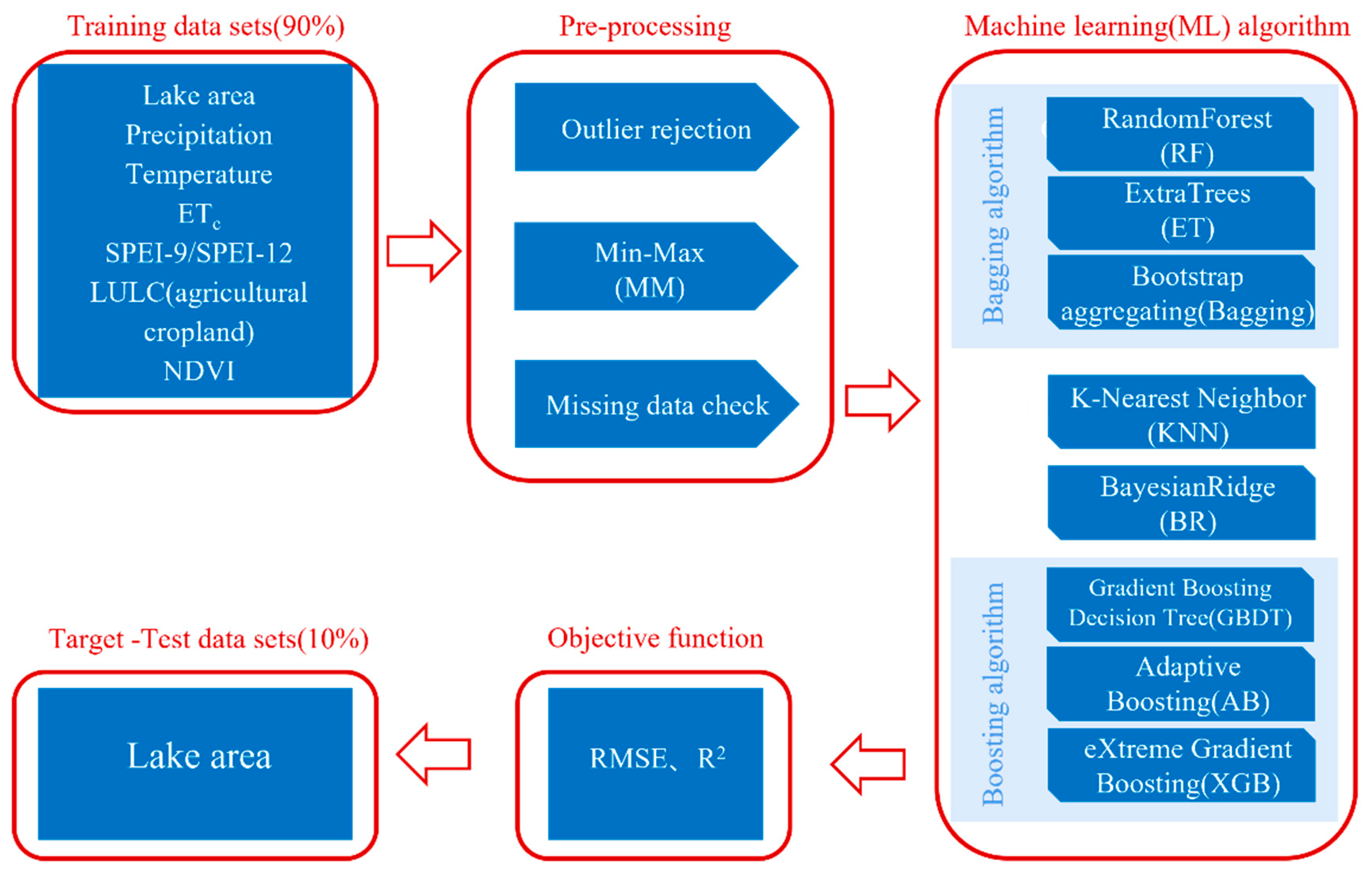
Figure 3 shows the workflow for the machine learning model used in this study. The important step is determining the predictor factor for monthly lake area. In our study area, the dynamics of lakes are influenced by meteorology and human activities, etc. As a result, SPEI, precipitation, temperature, NDVI, ETc, and LUCC were chosen as input variables of the ML model. The observed NDVI changes in the study area showed a clear seasonal pattern. As the NDVI value increased, more water resources were consumed by ETc, which led to a decrease in the groundwater level associated with the lake area. Therefore, NDVI can be used as an important indicator of lake area change. It is important to note that the study area’s geographical characteristics play a crucial role in local cultivation practices; groundwater is a vital resource in the region, and fluctuations in its availability can significantly affect the lake area. As a result, the land-use types included in the model are mainly agricultural croplands, reflecting the primary land use in the region.
In order to accurately reflect the effects of human activities, the researchers chose maize, a widely cultivated crop in the Mu Us Sandy Land, as the primary research object. To calculate the crop’s evapotranspiration, we used the single crop coefficient method, which is a widely accepted and precise method. Considering that precipitation is the main source of groundwater and lake recharge in the Mu Us Sandy Land, the study introduced precipitation and ETc as model predictor variables and added them to obtain monthly values, and then averaged them to obtain monthly average data. The study revealed that the rainfall distribution in the area is highly heterogeneous, with most of the rainfall concentrated in July and August. The rainfall mainly consisted of light rainfall with daily rainfall less than 10 mm and medium rainfall between 10 and 25 mm, with medium rainfall mainly distributed in July and August.

2.5.2. ML Algorithm

In this study, the entire dataset was divided into two subsets according to a 9:1 ratio, with the larger subset used for training the ML algorithm and the smaller subset used for testing. To ensure the validity of the modelling, different ratios, such as 80% and 70%, were tested, but the results did not show significant changes. The availability of large datasets reduced the risk of over-parameterisation, allowing for accurate and reliable results. The above process was implemented using the Scikit-Learn package for Python 3.7 [38]. ML performance was then checked using a test dataset to ensure that the calibrated parameters were not overfitting or underfitting the training results and could be used in other situations.

2.5.3. Training and Testing of ML Methods

The third step in the process is selecting the machine learning (ML) algorithm, which involves determining the structural hyperparameters that define the algorithm’s features. Additionally, coefficients specified in the algorithm’s equations, as outlined by [39], are chosen for individual case studies and input variable combinations. To optimise the hyperparameters, various methods such as grid search, stochastic search, Bayesian methods, and particle swarm optimisation (PSO) are employed. These techniques aid in fine-tuning the algorithm’s performance to achieve optimal results. Machine learning commonly uses optimisation methods to find the best models for a dataset, and grid search with five-fold cross-validation is a popular approach. This method is highly effective in providing optimal results while limiting computational cost [40].
The present study sought to explore the performance of eight different machine learning methods, namely, BR, KNN, GBDT, ET, RF, AB, Bagging, and XGB. This study employed a unified set of parameters for each machine learning method. This allowed for a more precise comparison of the models, eliminating any confounding variables that might have impacted the results. Overall, the use of grid search with fivefold cross-validation in conjunction with a standardised set of parameters for each machine learning method proved to be a highly effective approach in this study. The results obtained demonstrate the potential of these techniques in achieving optimal machine learning models with reasonable computational costs.

2.5.4. Model Validation

To compare model performance, four indices were used, including coefficient of determination (R2), root mean square error ( R M S E ), Lin’s concordance ( L C C C ), and ratio of performance to deviation ( R P D ). The formulas for the four indices are as follows:
(1)
Root mean square error or RMSE (km2):
R M S E = i = 1 n ( x i x ^ i ) 2 n
where in x i and x ^ i are the actual and predicted areas of the ith lake, respectively, and n is the total number of lakes. The greater the model prediction error, the greater the R M S E .
(2)
Coefficient of determination (R2):
R 2 = i = 1 n ( x i x ¯ ) ( x ^ i x ~ ) i = 1 n ( x i x ¯ ) 2 × i = 1 n ( x ^ i x ~ ) 2 2
where x ~ is the average predicted lake area. R2 shows the degree of co-linearity between the observed and simulated time series and has a range of 0.0–1.0, with higher values indicating a higher degree of co-linearity.
(3)
L C C C weights averaging:
Under L C C C weights averaging, the weight of the ith model ( w i ) is estimated as [41]:
w i = L C C C i i = 1 n L C C C i
where L C C C i is the L C C C of the ith model and n is the number of calibration samples.
L C C C = 2 l x y l x 2 + l y 2 + ( x ¯ y ¯ ) 2
where x i and y i are the actual and predicted lake areas; x ¯ and y ¯ are the means for x i and y i ; and l x 2 and l y 2 are the corresponding variances and
l x y = 1 n i = 1 n ( x i x ¯ ) ( y i y ¯ )
(4)
Ratio of performance to deviation ( R P D ):
The formula of R P D is as follows:
R P D = S D R M S E
where S D is the ratio of standard deviation and R M S E is the root mean square error.
According to Rossel et al. (2016) [42], an L C C C value of 1 indicates perfect agreement. An L C C C larger than 0.9 signifies excellent agreement, and a value ranging from 0.80 to 0.90 indicates good agreement. Moderate agreement is achieved when L C C C values are between 0.65 and 0.80, while values less than 0.65 denote poor agreement. The R P D provides an evaluation based on prediction accuracy, categorised from excellent ( R P D > 2.5), very good (2.0 < R P D < 2.5), good (1.8 < R P D < 2.0), fair (1.4 < R P D < 1.8), to poor ( R P D < 1.4). We considered the best prediction model to be the one with the largest R2, L C C C , and R P D values and the smallest R M S E , collectively providing a comprehensive assessment of the model’s performance.

3. Results

3.1. Lake Area Accuracy Assessment

Using the areas of 13 lakes in Mu Us Sandy Land in Wushen Banner from 2000 to 2017, as mentioned in the Wushen Banner Lake Water Ecological Comprehensive Management Plan, as the verification data of lakes extracted by remote sensing in this study (Figure 4), it can be seen that the extraction accuracy is R2 = 0.82. Larger errors occurred in 2000, 2001, and 2015. The total area of lakes in these three years was relatively small. It can be found that the extraction of lake area by remote sensing technology performed poorly when the value was small. Data after 2017 cannot currently be accurately verified with available data.
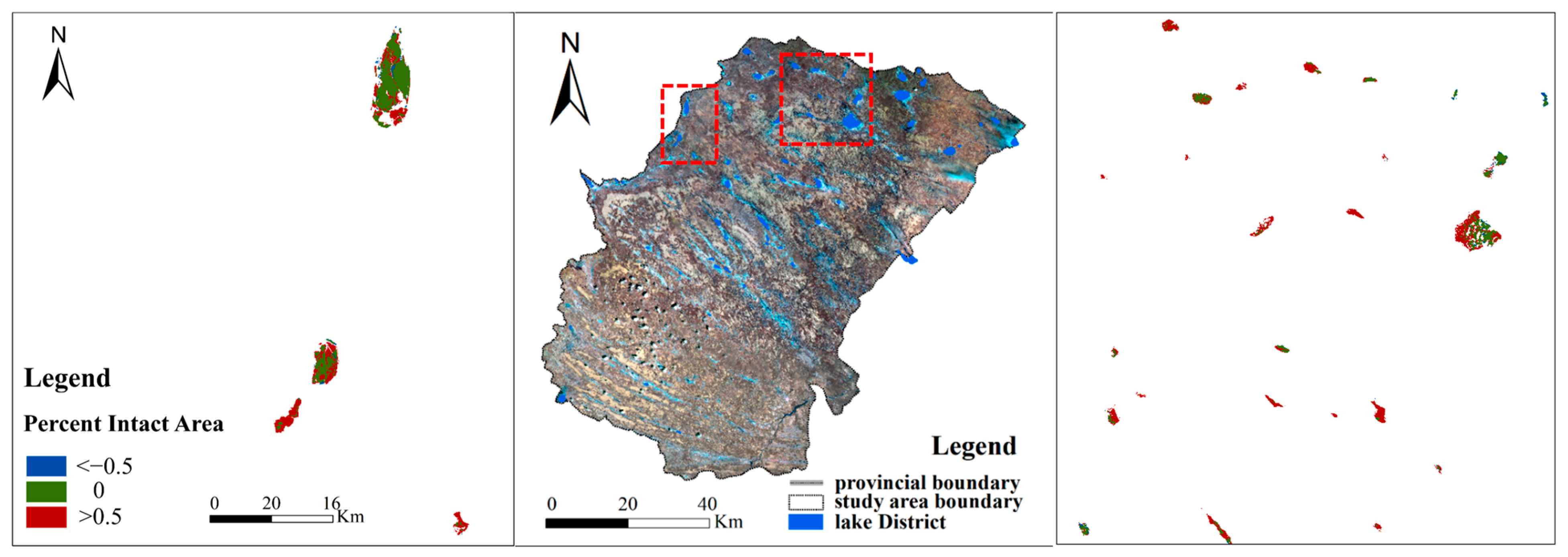
The long-term averages of the classified lakes from 2000 to 2020 revealed a notable change in spatial pattern. Based on the classification where water is assigned a value of 1 and no water is assigned a value of 0, areas with a consistent presence of water exhibit mean values closer to 1, while areas without water have mean values close to 0, indicating intermittent water presence. The fluctuations in the percentage of lake area in different banners within the Mu Us Sandy Land from 2000 to 2020 are presented in Table 3, highlighting the variability over time. YJHLQ had the highest percentage of lakes with fluctuations in lake area equal to or less than 20%. Conversely, ETKQQ and YC had the highest percentage of permanent lake fluctuations. Furthermore, Figure 5 provides a visual representation of the diverse responses of the larger lakes within the region to factors like drought. Notably, the alteration in lake area during the flat water period (September–October) exhibited an expanding trend over the last two decades. This trend can be attributed primarily to the influence of precipitation. Meteorological station precipitation data indicate a substantial increase in precipitation since 2016 compared to the period of 2000–2015. Within the Mu Us Sandy Land lakes complex, smaller lakes showed a noteworthy alteration, with a rate of change exceeding 0.5.
Anthropogenic disturbances within the region are regarded as potential drivers of these shifts. Activities such as hydraulic construction upstream, coal mining, construction of highways near the lakes, and irrigation water use could have impacted the dynamics of the lakes. These human-induced influences can disrupt natural hydrological processes, leading to modifications in water availability and the overall hydrological equilibrium.
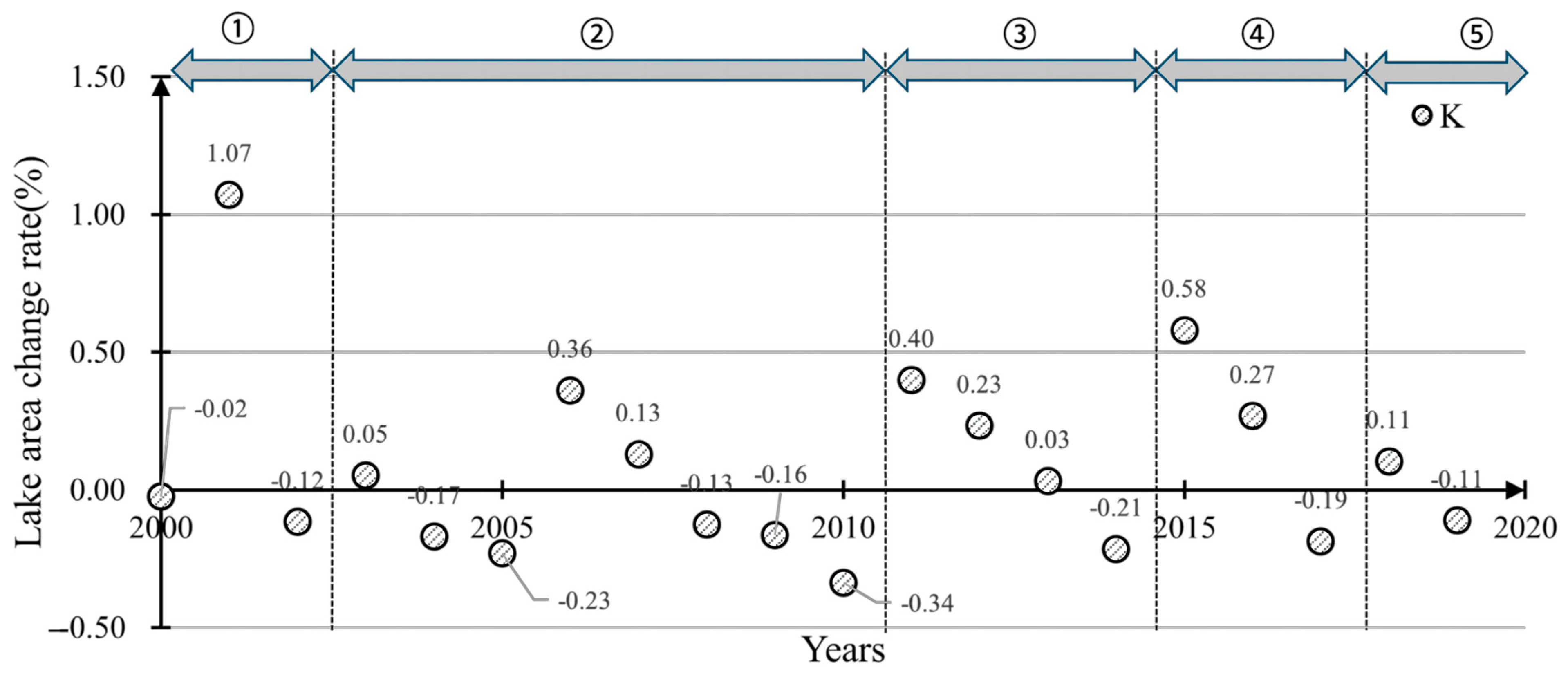
The temporal response of the lakes in the Mu Us Sandy Land revealed the seasonal, sudden, and long-term effects of drought. A closer analysis of the annual average value of the lake area from 2000 to 2020 unveiled five distinct stages (①–⑤ in Figure 6), each characterised by unique expansion and contraction patterns. The period from 2000 to 2002 represents a period of rapid expansion, indicating a sudden influx of water in the region. The following period, from 2003 to 2011, is marked by a slow contraction, as the water levels steadily decreased. In contrast, from 2012 to 2014, the area experienced a slow expansion phase, followed by a sharp expansion period from 2015 to 2017. Finally, from 2018 to 2020, the region entered another phase of slow contraction, further emphasising the long-term effects of drought.

3.2. SPEI Time Scale Decisions

The research aimed to create an optimal prediction model for lake area, and to achieve this, we conducted a correlation analysis between the SPEI of various time scales and the monthly lake area. The results are shown in Figure 7. The analysis revealed that the SPEI values at the 9-month and 12-month scales were better correlated with the lake area, indicating that these time scales are important predictors. Under the 9-month time scale, YC and ETKQ had a higher correlation with the lake area, with R values of 0.39 and 0.34, respectively. Similarly, under the 12-month time scale, WSQ and WSZ had a better correlation with lake area, with R values of 0.47 and 0.28, respectively. These findings suggest that the choice of different time scale SPEI variables could have a significant impact on the performance of ML models in reproducing lake area. The final selections of SPEI-9 and SPEI-12 were used as predictor variables to construct the models in Section 3.3, thus providing a more detailed understanding of the effects of input variables on model performance at different time scales. These results can help to develop more accurate and reliable prediction models for the Lake District.

3.3. The Performance of the ML Algorithm

A total of eight ML algorithms (BR, KNN, GBDT ET, RF AB, Bagging, XGB) were used to estimate the monthly lake area. Here, we employed two temporal-scale SPEIs, the 9-month scale (SPEI-9) and the 12-month scale (SPEI-12). The corresponding ML models were expressed as MLSPEI-9 and MLSPEI-12, respectively. To ensure a fair and unbiased comparison, the study implemented a standardised analysis procedure: the parameters used for model construction were all unified, and the better performing of the MLSPEI-9 and MLSPEI-12 models for the seven regions were optimised with a hyperparametric algorithm (grid search cross-validation method).
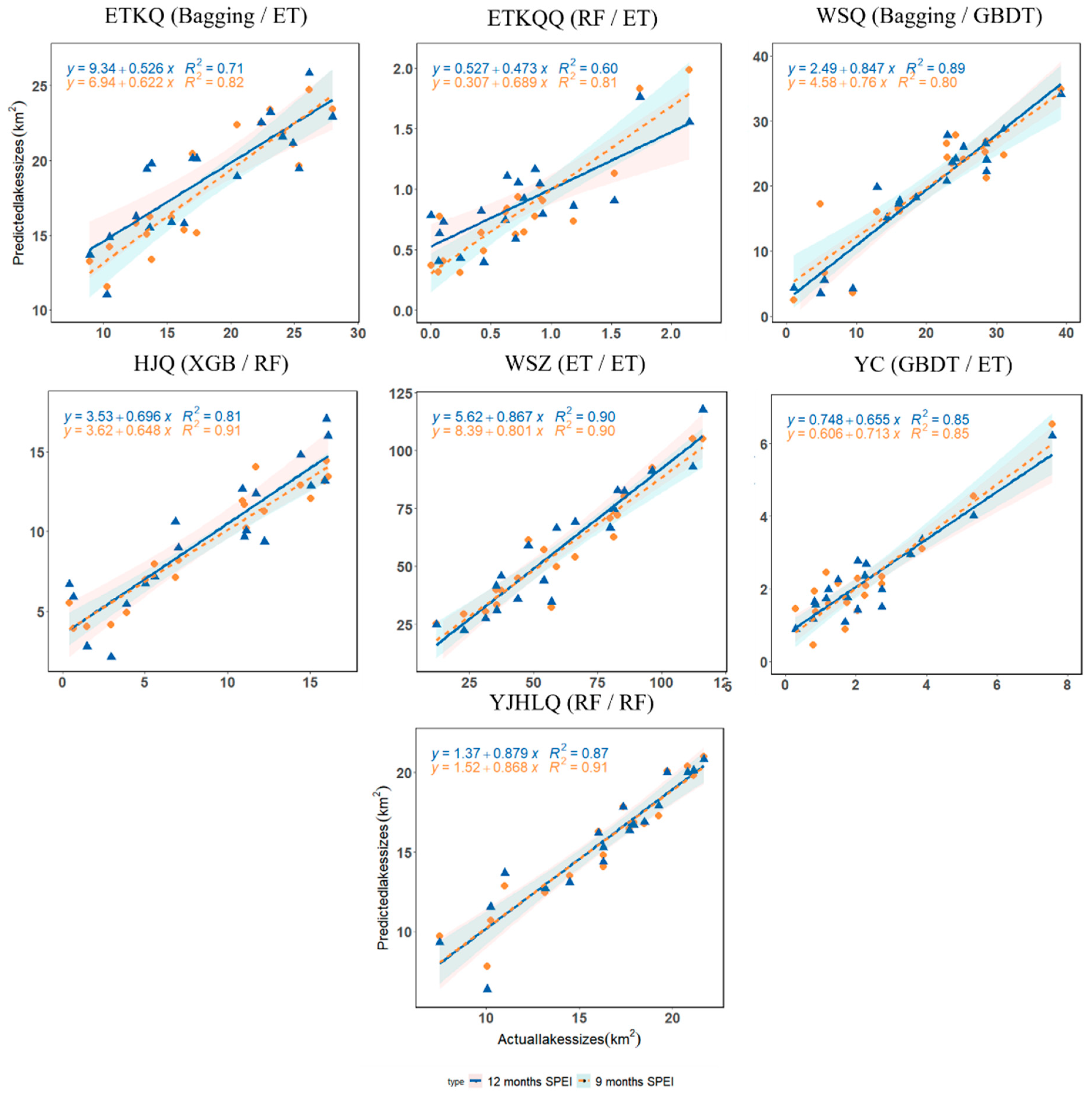
As shown in Table A1 (Appendix A) and Figure 8, there were some differences in the predictive ability of the eight algorithms for the area of the Mu Us Sandy lakes in the two scenarios. In general, the five models GBDT, ET, RF, Bagging, and XGB performed better. First, the better performers under MLSPEI-9 were mainly the GBDT, ET, RF, Bagging, and XGB models, with RMSEs ranging from 0.0 to 11.1 km2, R2 ranging from 0.70 to 0.99, LCCC ranging from 0.87 to 0.99, and RPD ranging from 0.0 to 58.1 for the training dataset, while the test dataset had RMSEs ranging from 0.2 to 14.5 km2, R2 from 0.51 to 0.88, LCCC ranging from 0.74 to 0.95, and RPD ranging from 8.3 to 2224.5 for the test dataset with the RF model performing the best in terms of predictive power. With the five models, the RMSE of the test set performed poorly in the WSZ (14.51/12.02/13.74/12.40/13.58 km2). The best-performing models in each region were optimised to improve their accuracy significantly, with a maximum reduction of 13.89% in RMSE and a maximum improvement of 6.58% in R2 for the optimised model test set.
The RF and Bagging models performed better in the study area under MLSPEI-12, with RMSEs in the range of 0.26 to 8.59 km2, R2 from 0.74 to 0.94, LCCC ranging from 0.09 to 0.99, and RPD ranging from 0.0 to 113.0 for the training dataset. The BR and KNN models performed worse in the WSZ (RMSE = 26.05/24.32 km2). The RMSEs for the test dataset ranged from 0.40 to 13.94 km2, R2 in the range of 0.45 to 0.88, LCCC in the range of 0.19 to 0.94, and RPD in the range of 9.4 to 2651.2. The RMSEs of the four models continued to perform poorly in the WSZ. Using the grid search cross-validation method to optimise the seven models that performed better in the region, it could be seen that for the test set, the RMSE values decreased by a maximum of 26.95% and the R2 improved by a maximum of 6.74%.
With the exception of RF, the three regression models, GBDT, ET and BR, all had relatively satisfactory accuracy on both the training and test datasets, but there were large deviations in predicting the area of small lake groups (e.g., the area of most of the lakes in ETKQQ is less than 1 km2), and the accuracy of the optimised models improved significantly, which was consistent with the change in lake area corresponding to the frequency of drought events. This implies that in this case, it is possible to achieve improved predictions without requiring extensive pre-processing of the data. It was of interest to interpret the performance of the ML method in light of its specific characteristics. For the eight classes of models selected for the study, RF can be seen as an extended variant of Bagging, where ET can be seen as an improved version of RF, which selects feature variables randomly and draws samples with random putbacks. A bootstrap method is utilised to select the sample set for training each decision tree. This means that for each decision tree in the ensemble, a random subset of the original training set is chosen with replacement using the bootstrap technique. In addition, in the RF method, the input samples are divided into subsamples by random sampling with replacement. This process allows for the possibility of duplicate data within each subsample. In contrast, the ET algorithm does not use random sampling with replacement, thereby avoiding data duplication [43]. Based on the findings of previous studies, the ET algorithm has been observed to be a more robust approach compared to RF. It exhibits a lower degree of performance degradation when transitioning from the training phase to the testing phase (since the division points of the eigenvalues are chosen randomly instead of the optimal points, this will result in the size of the generated decision trees being generally larger than those generated by RF). That is, the variance of the model is further reduced relative to RF, but the bias is further increased relative to RF. At some point, the generalisation ability of the ET is better than that of the RF, and in general, the extreme RF classifier outperforms the RF classifier in terms of classification accuracy and training time, etc. AB and GDBT are both members of the Boosting family, use weak classifiers, and both use forward distribution algorithms; the iterative ideas are different: AB compensates for the model’s shortcomings by boosting the weights of misclassified data points (using misclassified samples), while GBDT compensates for the model’s shortcomings by counting gradients (using residuals). The loss functions of the two are different: AB uses exponential loss, GBDT uses absolute loss or Huber loss function. Compared to AB, GBDT is recognised as a more generalisable algorithm, and in this study also showed a similarly strong regression prediction capability.

3.4. Performance of MLSPEI-9 and MLSPEI-12 Model to Estimate Lake Area

Validation of the lake areas predicted by MLSPEI-9 and MLSPEI-12 showed that MLSPEI-9 performed better in predicting the area of the Mu Us Sandy Land lakes complex, with R2 between simulated and true values ranging from 0.81 to 0.91, with the RF model performing best, reaching an R2 of 0.882 at YJHLQ for the optimised test dataset. The RMSE was 1.364 km2 (Figure 8 and Appendix A).
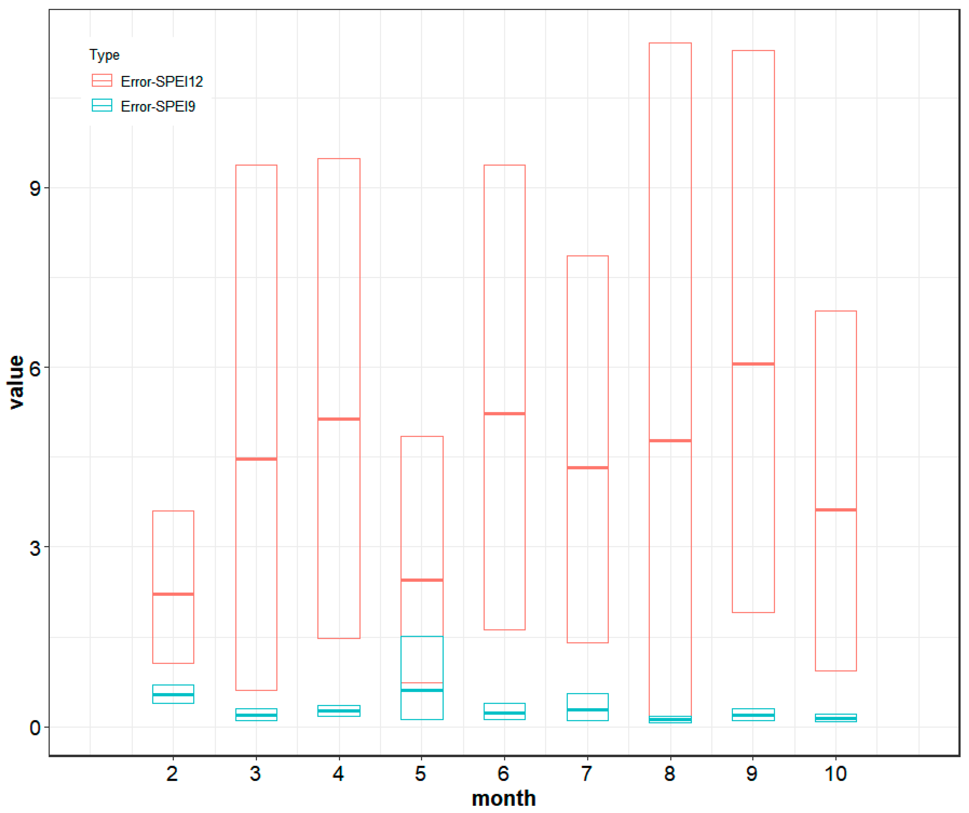
A seasonal analysis of the relative errors (mainly the maximum and minimum values as well as the mean values) on the 95% confidence interval by bootstrapping showed that (Figure 9) the relative error of MLSPEI-9 was much lower than that of MLSPEI-12, where the relative error of MLSPEI-12 was lower in February, May, and October and higher in August and September. The reason for this may be related to the strong human production and activity during this period, the gradual increase in the ecological water demand of vegetation, irrigation of farmland, and strong evapotranspiration, leading to drastic changes in the area of the lake group in summer. This was a test of the ML model’s ability to capture the sensitivity of prediction dynamics; the average relative errors of MLSPEI-9 were lower in March, August, September, and October, with relative errors ranging from 0.12 to 0.19, with the average maximum value of the relative error occurring in May, when the value reached 0.62.

4. Discussion

4.1. Advantages of ML in Regression Analysis

ML is a more successful method for predicting lake area and can effectively characterise lakes as influenced by various factors. Physically based hydrodynamic models are known for their complexity and the need to generate results based on assumed inputs, including information on lake morphology, inflow and outflow conditions, and a comprehensive range of meteorological variables such as air temperature, precipitation, and wind, whereas machine learning models require empirical data for training and subsequent predictions. It is essential to note that without adequate data, machine learning models lack the foundational information required for generating meaningful insights. Conversely, physics-based models leverage established physical principles to generate results, yet the accuracy of these results still hinges on the accuracy of the input data. However, this data-intensive requirement can make the application of physical models impractical, especially in regions with limited data availability. To overcome this limitation, researchers have increasingly turned to the development and utilisation of machine learning models for lake area forecasting. One notable advantage of these machine learning models is their relatively lower data requirements as inputs, as highlighted in studies by Kisi et al. (2015), Li et al. (2016), and Shiri et al. (2016) [44,45,46]. In recent decades, various types of machine learning models have been devised and employed in hydrological and environmental research, offering promising solutions to the challenges posed by data scarcity and complexity [47,48,49,50,51,52,53]. In this study, the performance of eight machine learning models was examined to leverage the advantages of machine learning in predicting lake area. However, it should be noted that further investigations are required to explore the existence of potentially superior machine learning models in future studies.

4.2. Variation in the Performance of Different MLs in Different Regions

This study used eight machine learning models for lake area prediction in seven different regions, and the results of the study indicated that a group of methods performed reasonably well in a given region, and in general, the eight ML models had better simulation accuracy on larger lakes, e.g., WSZ. According to the findings of Zhang et al. (2009) [54], the response of lakes is influenced by their size. Larger lakes tend to exhibit greater sensitivity to long-term climate effects, which can manifest as gradual changes over time. These lakes may moderate the impact of seasonal variations on their water levels or area. On the other hand, smaller lakes are found to be more responsive to seasonal effects, showing more pronounced fluctuations in water levels or area in response to short-term climate variations throughout the year. This research highlights the importance of considering lake size as a factor in understanding and predicting the responses of lakes to climate dynamics. While KNN generally performed poorly in the eight regions, overall, RF performed best in the study area. It was found that models like the more current XGB did not stand out, while the more traditional RF model instead delivered satisfactory results, thanks to the advantages of the Random Forest algorithm itself, such as high accuracy, wide applicability, strong non-linear data analysis, and less susceptibility to overfitting [55], suggesting that traditional methods sometimes perform better than advanced algorithms. This study only focused on lake area prediction in the Mu Us Sandy Land, which has some limitations, and the applicability of the model to other regions remains to be explored.

4.3. The Determination of Input Factors Is Key to the Accuracy of the Prediction Results

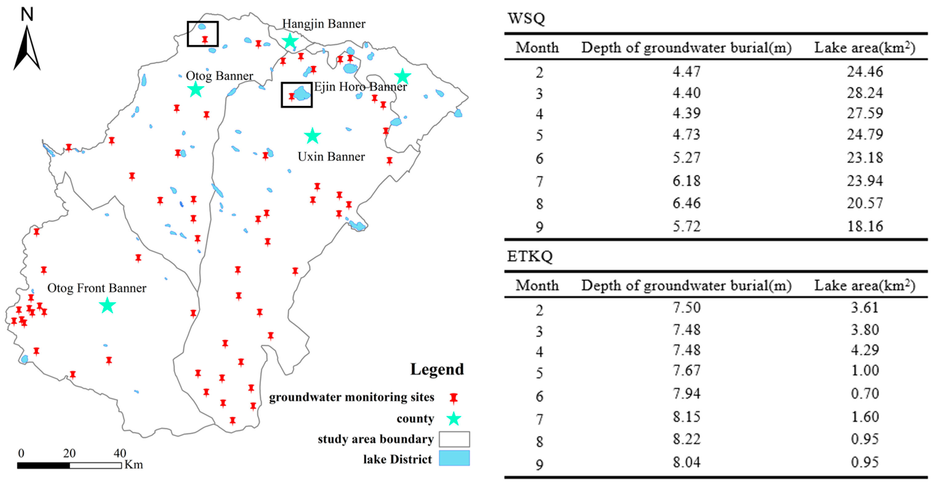
The selection of input factors is key to the accuracy of prediction, and owing to the limitations of the acquired data, the important factors affecting lake area response were morphological and hydrological characteristics, and the depth of groundwater burial was not considered as a predictive variable in this study. Groundwater plays an important role in lakes in arid and semi-arid regions. In cases where evapotranspiration surpasses precipitation, any deficit in the water balance of the lake is compensated for by the contribution of groundwater. The variability in water table depth, aquifer thickness, and hydraulic connectivity unveiled spatial and temporal patterns within the complex of lakes in the Mu Us Sandy Land region. Additionally, research has indicated that the size of lakes in arid and semi-arid areas is influenced by factors such as the gradient of groundwater flow [56,57], the positioning of the lake relative to local or regional groundwater flow [58], storage capacity, lake bathymetry [59], as well as topography and geographical characteristics of the area. These factors collectively play a role in shaping the dynamics and area of lakes in arid and semi-arid regions [60,61,62,63]. It was evident from this study that climatic and anthropogenic influences cause smaller shallow lakes to dry up immediately during droughts and larger lakes to decrease in size. Therefore, whether fluctuations in lake area in the Mu Us Sandy Land can be used as an entry point for measuring and monitoring changes in precipitation and groundwater levels in the Mu Us Sandy Land is a focus for future research. A lake closer to the groundwater monitoring point was selected in each of the Otog Banner and Uxin Banner areas, and the area of the two lakes from February to October 2021 was extracted using the latest JRC Monthly Water History v1.4 dataset available in GEE. Analysis with the groundwater monitoring point data showed that the lake area has a trend of decreasing with the increase in groundwater burial depth (Figure 10). This indicates that there is a correlation between lake area and groundwater depth in the Mu Us Sandy Land. As the 29 groundwater monitoring sites in the region started to provide data in 2019, the regression model of this study did not introduce groundwater depth data as a driving variable in view of the lack of continuity of data. Future research will discuss the feasibility and optimisation effects of introducing groundwater depth of burial data to drive the lake area prediction model.

4.4. Accuracy and Limitations of JRC Dataset in Identifying Water Bodies at 30 m Resolution

The overall accuracy of the JRC dataset in identifying water bodies was higher. This heightened accuracy (>95%) results from the combination of the drooling cap component, original strips, and the pronounced contrast between water and the homogeneous surrounding landscape. Given a spatial resolution of 30 m, at least nine pixels are required to consistently represent an object using Landsat imagery [64]. To circumvent mixed pixel effects caused by suspended sediment, submerged or floating vegetation, and background reflectivity at lake boundaries, the pixels within the 3*3 filter were removed, leading to an underrepresentation of smaller lakes. Likewise, the non-uniform distribution and limited number of cloud-free images hindered capturing the seasonal variations within the smaller lakes of the Mu Us Sandy Land. Consequently, this study’s response to the spatial and temporal variability of smaller lakes is localised or limited. Nonetheless, the results suggest that higher-resolution satellites (e.g., Sentinel-2) could be leveraged to characterise smaller lakes and their responses to seasonal variability. However, many high-resolution satellites exhibit limitations in terms of time (revisit frequency) and recording periods.

4.5. Assessing the Use of Drought Indices and Potential of Lakes as Monitoring Wells in the Mu Us Sandy Land

While the SPEI effectively mirrors the precipitation conditions in the Mu Us Sandy Land region, further exploration is needed for drought indices such as the SPI. Subsequent investigations should consider the impact of local hydraulic conductivity, regional lake location, and topography on changes in lake response. Given the sporadic nature of monitoring well data in the Mu Us Sandy Land area, future research could explore the feasibility of utilising lakes as monitoring ‘wells’ to enhance the quantification of groundwater levels.

5. Conclusions

This study aimed to investigate the potential of using machine learning (ML) methods to predict the monthly lake area in a typical arid area. The input variables for these ML models included both meteorological factors and human activities data. The conclusions drawn from the study are as follows:
  • ML Models’ Performance: Eight different ML algorithms were utilised to predict the lake area based on the given input variables. The results indicate that all eight ML methods were able to effectively describe the relationship between lake area and both meteorological factors and human activities. This implies that ML models can be utilised to understand and predict the response of lake areas to various environmental and anthropogenic factors.
  • Superiority of the RF Model: Among the various ML algorithms tested, the RF model emerged as the most robust performer. Its performance was quantified using the R2, and the RF model achieved an impressive R2 value of 0.88. This indicates that the RF model’s predictions closely matched the observed lake area data, making it a reliable tool for predicting lake area in the study area.
  • Limited Performance of the BR and KNN Models: On the other hand, the study found that the BR and KNN models consistently provided poorer results compared to the other ML algorithms tested. These models may not capture the complex relationships between lake area and the predictor variables as effectively as the RF and other models.
  • Importance of Meteorological Factors: The study also explored the impact of different meteorological factors on the lake area prediction. Specifically, the SPEI at various time scales was introduced as an input variable. The analysis revealed that SPEI-9, which represents a longer-term climate condition, had a positive effect on predicting lake area. This suggests that long-term meteorological patterns play a significant role in determining lake area variations in the arid area under investigation.
  • Identifying Appropriate Predictor Variables: The success of applying ML algorithms to predict lake area largely depends on the selection of suitable predictor variables. This study emphasises the importance of including both meteorological and human activity factors in the inputs to achieve accurate predictions.
Overall, this study provides valuable insights into the effects of using SPEI as predictors at different time scales and the performance of various ML algorithms in predicting lake area in arid regions. The findings can serve as a guide for future research in lake area prediction, and researchers can utilise the results to make informed choices regarding model selection and predictor variables to enhance the accuracy of their predictions.

Author Contributions

Conceptualization, D.W. and Z.H.; Methodology, D.W. and Z.H.; Software, D.W., Z.H., P.M. and X.T.; Formal analysis, D.W. and Z.H.; Investigation, P.M.; Data curation, D.W.; Writing—original draft, D.W.; Writing—review & editing, D.W., Z.H., P.M. and X.T.; Project administration, Z.H.; Funding acquisition, Z.H. All authors have read and agreed to the published version of the manuscript.

Funding

This research was funded by A special project entitled Science and Technology for the Development of Mongolia, Department of Science and Technology of Inner Mongolia, Grant No. 2021EEDSCXSFOZD010.

Data Availability Statement

The data presented in this study are available on request from the corresponding author.

Conflicts of Interest

The authors declare no conflict of interest.

Appendix A

Table A1. Performance of eight machine learning models in predicting the area of the Mu Us Sandy Land lakes complex under SPEI-9 and SPEI-12, respectively (values in brackets correspond to test data, bolded italics are the optimal prediction models for the 7 regions).
SPEI-9
ETKQETKQQHJQWSZWSQYCYJHLQ
RMSER2RMSER2RMSER2RMSER2RMSER2RMSER2RMSER2
BayesianRidg5.896
(5.148)
0.084
(0.231)
0.678
(0.483)
0.040
(0.286)
4.676
(5.339)
0.003
(−0.002)
26.17
(26.291)
0.208
(0.172)
8.402
(7.576)
0.233
(0.397)
1.165
(1.281)
0.417
(0.441)
4.423
(3.849)
0.075
(0.058)
KNN4.982
(5.268)
0.346
(0.195)
0.596
(0.504)
0.258
(0.219)
3.610
(3.601)
0.406
(0.544)
24.31
(26.297)
0.317
(0.172)
7.909
(10.447)
0.320
(−0.146)
1.201
(1.509)
0.380
(0.225)
3.632
(3.354)
0.376
(0.285)
GBDT0.164
(3.805)
0.999
(0.580)
0.032
(0.349)
0.998
(0.627)
0.149
(2.537)
0.999
(0.774)
0.694
(14.511)
0.999
(0.748)
0.382
(4.351)
0.998
(0.801)
0.032
(0.813)
0.999
(0.775)
0.126
(2.231)
0.999
(0.683)
ET2.745
(3.042)
0.801
(0.731)
0.378
(0.277)
0.702
(0.765)
2.535
(2.802)
0.707
(0.724)
11.12
(12.020)
0.857
(0.827)
4.530
(5.604)
0.777
(0.670)
0.629
(1.054)
0.830
(0.622)
1.841
(1.802)
0.840
(0.793)
RF2.834
(3.549)
0.788
(0.635)
0.318
(0.307)
0.788
(0.712)
2.318
(2.315)
0.755
(0.812)
9.886
(13.735)
0.887
(0.774)
4.221
(4.195)
0.809
(0.796)
0.592
(0.951)
0.849
(0.692)
1.630
(1.382)
0.874
(0.879)
AB3.760
(3.899)
0.627
(0.559)
0.464
(0.405)
0.551
(0.498)
2.901
(3.127)
0.616
(0.656)
14.023
(14.519)
0.773
(0.748)
5.303
(5.878)
0.694
(0.637)
0.807
(0.964)
0.720
(0.684)
2.365
(2.100)
0.736
(0.719)
Bagging2.090
(3.481)
0.885
(0.648)
0.247
(0.315)
0.872
(0.695)
1.814
(2.392)
0.850
(0.799)
8.589
(12.395)
0.915
(0.816)
3.579
(4.693)
0.861
(0.769)
0.560
(1.036)
0.865
(0.635)
1.369
(2.138)
0.911
(0.709)
XGB0.001
(3.680)
0.999
(0.563)
0.001
(0.402)
0.999
(0.505)
0.001
(2.484)
0.999
(0.783)
0.001
(13.577)
0.999
(0.779)
0.001
(4.632)
0.999
(0.774)
0.001
(1.006)
0.999
(0.655)
0.001
(2.058)
0.999
(0.731)
grid search cross-validation1.529
(2.819)
0.938
(0.769)
0.223
(0.272)
0.895
(0.773)
1.835
(2.214)
0.846
(0.828)
6.366
(10.351)
0.953
(0.872)
0.653
(4.344)
0.995
(0.802)
8.403
(0.714)
0.999
(0.826)
1.477
(1.364)
0.897
(0.882)
SPEI-9
ETKQETKQQHJQWSZWSQYCYJHLQ
LCCCPRDLCCCPRDLCCCPRDLCCCPRDLCCCPRDLCCCPRDLCCCPRD
BayesianRidg0.302
(0.658)
113.1
(30.5)
0.211
(0.860)
/
(2224.5)
0.094
(0.524)
/
(259.8)
0.461
(0.544)
61.1
(43.0)
0.487
(0.726)
/
(103.8)
0.646
(0.682)
/
(67.1)
0.278
(0.247)
/
(23.6)
KNN0.594
(0.444)
95.8
(29.0)
0.509
(0.494)
/
(875.7)
0.644
(0.776)
/
(136.9)
0.567
(0.448)
53.1
(47.2)
0.569
(0.120)
/
(1123.6)
0.631
(0.506)
/
(65.9)
0.619
(0.634)
/
(16.8)
GBDT0.999
(0.767)
2.0
(17.4)
0.999
(0.796)
/
(965.6)
0.999
(0.914)
/
(79.068)
0.999
(0.905)
1.4
(16.3)
0.999
(0.897)
/
(31.8)
0.999
(0.900)
/
(60.2)
0.999
(0.861)
/
(12.6)
ET0.921
(0.907)
47.9
(16.3)
0.884
(0.923)
/
(1314.4)
0.881
(0.922)
/
(115.1)
0.938
(0.941)
25.3
(21.3)
0.914
(0.843)
/
(70.4)
0.929
(0.835)
/
(60.7)
0.930
(0.913)
/
(9.1)
RF0.910
(0.802)
58.1
(16.6)
0.926
(0.864)
/
(1331.4)
0.899
(0.951)
/
(120.1)
0.949
(0.921)
23.1
(23.0)
0.923
(0.897)
/
(37.8)
0.946
(0.888)
/
(53.9)
0.946
(0.951)
/
(8.3)
AB0.843
(0.826)
44.0
(20.9)
0.817
(0.830)
/
(1657.6)
0.840
(0.897)
/
(138.5)
0.892
(0.920)
32.6
(26.2)
0.874
(0.814)
/
(60.3)
0.886
(0.897)
/
(57.2)
0.896
(0.945)
/
(11.4)
Bagging0.948
(0.818)
41.5
(16.3)
0.872
(0.845)
/
(1030.9)
0.932
(0.914)
/
(110.8)
0.962
(0.938)
18.0
(21.7)
0.940
(0.878)
/
(34.8)
0.938
(0.819)
/
(64.9)
0.959
(0.865)
/
(13.3)
XGB0.999
(0.785)
0.01
(16.9)
0.999
(0.742)
/
(2224.5)
0.999
(0.913)
/
(90.9)
0.999
(0.913)
0.002
(18.8)
0.999
(0.883)
/
(30.6)
0.999
(0.819)
/
(69.6)
0.999
(0.900)
/
(11.2)
grid search cross-validation0.976
(0.903)
18.4
(14.8)
0.963
(0.900)
/
(1182.4)
0.946
(0.956)
/
(115.3)
0.979
(0.948)
13.1
(18.4)
0.998
(0.897)
/
(32.9)
0.999
(0.922)
/
(55.7)
0.958
(0.952)
/
(8.6)
SPEI-12
ETKQETKQQHJQWSZWSQYCYJHLQ
RMSER2RMSER2RMSER2RMSER2RMSER2RMSER2RMSER2
BayesianRid5.903
(5.179)
0.081
(0.222)
0.678
(0.482)
0.040
(0.286)
4.676
(5.339)
0.003
(−0.002)
26.05
(26.345)
0.215
(0.169)
8.049
(5.974)
0.296
(0.625)
1.218
(1.294)
0.362
(0.430)
4.423
(3.849)
0.075
(0.058)
KNN4.979
(5.268)
0.347
(0.195)
0.597
(0.504)
0.256
(0.219)
3.620
(3.601)
0.402
(0.544)
24.32
(26.954)
0.316
(0.130)
7.896
(10.211)
0.323
(−0.095)
1.199
(1.509)
0.381
(0.225)
3.641
(3.354)
0.373
(0.285)
GBDT0.269
(4.565)
0.998
(0.395)
0.030
(0.451)
0.998
(0.376)
0.184
(3.194)
0.998
(0.641)
0.684
(14.171)
0.999
(0.759)
0.287
(3.694)
0.999
(0.857)
0.040
(0.789)
0.999
(0.788)
0.113
(2.288)
0.999
(0.667)
ET2.989
(3.535)
0.764
(0.637)
0.388
(0.412)
0.686
(0.479)
2.506
(3.049)
0.714
(0.673)
9.604
(11.882)
0.893
(0.831)
4.152
(3.855)
0.813
(0.844)
0.645
(1.159)
0.821
(0.542)
1.868
(1.804)
0.835
(0.793)
RF3.005
(3.507)
0.762
(0.643)
0.331
(0.398)
0.771
(0.513)
2.404
(3.136)
0.736
(0.654)
8.594
(13.938)
0.915
(0.767)
3.728
(3.472)
0.849
(0.873)
0.614
(1.095)
0.838
(0.592)
1.622
(1.526)
0.876
(0.852)
AB3.961
(4.321)
0.586
(0.458)
0.446
(0.447)
0.586
(0.388)
2.927
(3.216)
0.609
(0.637)
13.52
(15.019)
0.789
(0.730)
5.394
(5.116)
0.684
(0.725)
0.781
(1.104)
0.737
(0.585)
2.487
(2.420)
0.708
(0.628)
Bagging2.026
(3.135)
0.892
(0.715)
0.262
(0.423)
0.857
(0.452)
1.839
(3.368)
0.846
(0.601)
7.088
(13.392)
0.942
(0.785)
3.271
(3.392)
0.884
(0.879)
0.525
(1.049)
0.881
(0.626)
1.428
(1.772)
0.904
(0.800)
XGB0.001
(3.793)
0.99
9(0.582)
0.001
(0.477)
0.999
(0.303)
0.001
(2.781)
0.999
(0.728)
0.001
(13.292)
0.999
(0.788)
0.001
(3.875)
0.999
(0.842)
0.001
(1.099)
0.999
(0.589)
0.001
(2.279)
0.999
(0.670)
grid search cross-validation1.279
(2.290)
0.913
(0.731)
0.234
(0.396)
0.886
(0.520)
0.001
(2.544)
0.999
(0.773)
3.696
(9.703)
0.984
(0.887)
2.924
(3.369)
0.907
(0.881)
0.100
(0.755)
0.996
(0.806)
1.300
(1.519)
0.920
(0.853)
SPEI−12
ETKQETKQQHJQWSZWSQYCYJHLQ
LCCCPRDLCCCPRDLCCCPRDLCCCPRDLCCCPRDLCCCPRDLCCCPRD
BayesianRid0.299
(0.645)
113.0
(30.7)
0.211
(0.859)
/
(2224.4)
0.094
(0.524)
/
(259.8)
0.468
(0.530)
60.9
(42.5)
0.547
(0.871)
/
(82.5)
0.603
(0.705)
/
(60.8)
0.278
(0.248)
/
(23.6)
KNN0.594
(0.444)
95.8
(29.0)
0.506
(0.494)
/
(875.7)
0.641
(0.776)
/
(136.9)
0.566
(0.399)
53.1
(48.8)
0.572
(0.192)
/
(119.0)
0.631
(0.505)
/
(66.0)
0.616
(0.634)
/
(16.8)
GBDT0.999
(0.636)
3.2
(23.6)
0.999
(0.653)
/
(2262.8)
0.999
(0.835)
/
(151.8)
0.999
(0.887)
1.283
(18.2)
0.999
(0.930)
/
(23.8)
0.999
(0.910)
/
(50.6)
0.999
(0.845)
/
(12.7)
ET0.897
(0.862)
50.4
(20.5)
0.887
(0.768)
/
(2221.1)
0.878
(0.879)
/
(142.0)
0.953
(0.924)
22.8
(20.2)
0.923
(0.930)
/
(52.1)
0.929
(0.798)
/
(56.3)
0.929
(0.913)
/
(9.7)
RF0.904
(0.857)
55.2
(19.8)
0.92
(0.792)
/
(2433.6)
0.887
(0.858)
/
(155.5)
0.963
(0.892)
19.9
(22.8)
0.936
(0.938)
/
(29.9)
0.946
(0.832)
/
(51.9)
0.947
(0.935)
/
(9.4)
AB0.818
(0.719)
39.3
(23.9)
0.81
(0.753)
/
(2634.2)
0.823
(0.860)
/
(138.1)
0.907
(0.913)
31.9
(28.3)
0.872
(0.876)
/
(60.4)
0.902
(0.850)
/
(67.0)
0.912
(0.893)
/
(12.8)
Bagging0.954
(0.853)
38.4
(17.1)
0.942
(0.714)
/
(2462.3)
0.929
(0.815)
/
(130.7)
0.973
(0.888)
15.8
(24.5)
0.944
(0.941)
/
(33.1)
0.950
(0.841)
/
(56.8)
0.954
(0.909)
/
(10.9)
XGB0.999
(0.773)
0.01
(19.9)
0.999
(0.655)
/
(2651.2)
0.999
(0.885)
/
(150.6)
1.000
(0.903)
0.002
(20.9)
0.999
(0.920)
/
(23.9)
0.999
(0.769)
/
(60.8)
0.999
(0.867)
/
(11.9)
grid search cross-validation0.954
(0.866)
47.8
(17.8)
0.965
(0.848)
/
(1958.0)
0.999
(0.903)
/
(142.9)
0.993
(0.946)
7.8
(18.0)
0.964
(0.941)
/
(29.5)
0.998
(0.923)
/
(46.1)
0.969
(0.935)
/
(9.6)

References

  1. Wanders, N.; Wada, Y.; Van Lanen, H.A.J. Global hydrological droughts in the 21st century under a changing hydrological regime. Earth Syst. Dyn. 2015, 6, 1–15. [Google Scholar] [CrossRef]
  2. Gao, H. Satellite remote sensing of large lakes and reservoirs: From elevation and area to storage. WIREs Water 2015, 2, 147–157. [Google Scholar] [CrossRef]
  3. Venegas-Quiñones, H.L.; Thomasson, M.; Garcia-Chevesich, P.A. Water Scarcity or Drought? The cause and solution for the lack of water in laguna de aculeo. Water Conserv. Manag. 2020, 4, 42–50. [Google Scholar] [CrossRef]
  4. Fuentealba, M.; Latorre, C.; Frugone-Álvarez, M.; Sarricolea, P.; Giralt, S.; Contreras-Lopez, M.; Prego, R.; Bernárdez, P.; Valero-Garcés, B. A combined approach to establishing the timing and magnitude of anthropogenic nutrient alteration in a mediterranean coastal lake- watershed system. Sci. Rep. 2020, 10, 1–13. [Google Scholar] [CrossRef]
  5. Xu, F.; Bao, H.X.; Li, H.; Kwan, M.-P.; Huang, X. Land use policy and spatiotemporal changes in the water area of an arid region. Land Use Policy 2016, 54, 366–377. [Google Scholar] [CrossRef]
  6. Yan, D.; Xu, H.; Lan, J.; Zhou, K.; Ye, Y.; Zhang, J.; An, Z.; Yeager, K.M. Solar activity and the westerlies dominate decadal hydroclimatic changes over arid Central Asia. Glob. Planet. Chang. 2019, 173, 53–60. [Google Scholar] [CrossRef]
  7. Zhang, F.; Kung, H.-T.; Johnson, V.C. Assessment of Land-Cover/Land-Use Change and Landscape Patterns in the Two National Nature Reserves of Ebinur Lake Watershed, Xinjiang, China. Sustainability 2017, 9, 724. [Google Scholar] [CrossRef]
  8. Zhao, D.; Arshad, M.; Wang, J.; Triantafilis, J. Soil exchangeable cations estimation using Vis-NIR spectroscopy in different depths: Effects of multiple calibration models and spiking. Comput. Electron. Agric. 2021, 182, 105990. [Google Scholar] [CrossRef]
  9. Lu, S.; Ouyang, N.; Wu, B.; Wei, Y.; Tesemma, Z. Lake water volume calculation with time series remote-sensing images. Int. J. Remote. Sens. 2013, 34, 7962–7973. [Google Scholar] [CrossRef]
  10. Baup, F.; Frappart, F.; Maubant, J. Combining high-resolution satellite images and altimetry to estimate the volume of small lakes. Hydrol. Earth Syst. Sci. 2014, 18, 2007–2020. [Google Scholar] [CrossRef]
  11. Ovakoglou, G.; Alexandridis, T.K.; Crisman, T.L.; Skoulikaris, C.; Vergos, G.S. Use of MODIS satellite images for detailed lake morphometry: Application to basins with large water level fluctuations. Int. J. Appl. Earth Obs. Geoinf. 2016, 51, 37–46. [Google Scholar] [CrossRef]
  12. Yao, F.; Wang, J.; Wang, C.; Crétaux, J.-F. Constructing long-term high-frequency time series of global lake and reservoir areas using Landsat imagery. Remote. Sens. Environ. 2019, 232, 111210. [Google Scholar] [CrossRef]
  13. Guo, F.J.; Li, T.; Ji, M. Time series analysis and prediction of Qinghai Lake area from 2000 to 2019. Sci. Technol. Eng. 2022, 22, 740–748. [Google Scholar]
  14. Harris, A.R.; Mason, I.M. Lake area measurement using AVHRR A case study. Int. J. Remote Sens. 1989, 10, 885–895. [Google Scholar] [CrossRef]
  15. Zeng, Z.P.; Lu, X.H. Spatial-temporal evolution of urban lakes in Wuhan City based on remote sensing images. J. Lake Sci. 2008, 20, 648–654. [Google Scholar]
  16. Karpatne, A.; Ebert-Uphoff, I.; Ravela, S.; Babaie, H.A.; Kumar, V. Machine Learning for the Geosciences: Challenges and Opportunities. IEEE Trans. Knowl. Data Eng. 2018, 31, 1544–1554. [Google Scholar] [CrossRef]
  17. Chadalawada, J.; Herath, H.M.V.V.; Babovic, V. Hydrologically Informed Machine Learning for Rainfall-Runoff Modeling: A Genetic Programming-Based Toolkit for Automatic Model Induction. Water Resour. Res. 2020, 56. [Google Scholar] [CrossRef]
  18. Herath, H.M.V.V.; Chadalawada, J.; Babovic, V. Hydrologically informed machine learning for rainfall–runoff modelling: Towards distributed modelling. Hydrol. Earth Syst. Sci. 2021, 25, 4373–4401. [Google Scholar] [CrossRef]
  19. Cai, H.; Liu, S.; Shi, H.; Zhou, Z.; Jiang, S.; Babovic, V. Toward improved lumped groundwater level predictions at catchment scale: Mutual integration of water balance mechanism and deep learning method. J. Hydrol. 2022, 613, 128495. [Google Scholar] [CrossRef]
  20. Reichstein, M.; Camps-Valls, G.; Stevens, B.; Jung, M.; Denzler, J.; Carvalhais, N.; Prabhat, F. Deep learning and process understanding for data-driven Earth system science. Nature 2019, 566, 195–204. [Google Scholar] [CrossRef]
  21. Shrestha, N.; Mittelstet, A.R.; Gilmore, T.E.; Zlotnik, V.; Neale, C.M. Effects of drought on groundwater-fed lake areas in the Nebraska Sand Hills. J. Hydrol. Reg. Stud. 2021, 36, 100877. [Google Scholar] [CrossRef]
  22. Poul, A.K.; Shourian, M.; Ebrahimi, H. A Comparative Study of MLR, KNN, ANN and ANFIS Models with Wavelet Transform in Monthly Stream Flow Prediction. Water Resour. Manag. 2019, 33, 2907–2923. [Google Scholar] [CrossRef]
  23. Koranga, M.; Pant, P.; Kumar, T.; Pant, D.; Bhatt, A.K.; Pant, R. Efficient water quality prediction models based on machine learning algorithms for Nainital Lake, Uttarakhand. Mater. Today Proc. 2022, 57, 1706–1712. [Google Scholar] [CrossRef]
  24. Maier, P.M.; Keller, S. Estimating chlorophyll a concentrations of several inland waters with hyperspectral data and machine learning models. arXiv 2019, arXiv:1904.02052. [Google Scholar]
  25. Chen, H.; Yunus, A.P.; Nukapothula, S.; Avtar, R. Modelling Arctic coastal plain lake depths using machine learning and Google Earth Engine. Phys. Chem. Earth Parts A/B/C 2022, 126, 103138. [Google Scholar] [CrossRef]
  26. Ahirwal, J.; Nath, A.; Brahma, B.; Deb, S.; Sahoo, U.K.; Nath, A.J. Patterns and driving factors of biomass carbon and soil organic carbon stock in the Indian Himalayan region. Sci. Total Environ. 2021, 770, 145292. [Google Scholar] [CrossRef]
  27. Ngo, G.; Beard, R.; Chandra, R. Evolutionary bagging for ensemble learning. Neurocomputing 2022, 510, 1–14. [Google Scholar] [CrossRef]
  28. Ma, M.; Zhao, G.; He, B.; Li, Q.; Dong, H.; Wang, S.; Wang, Z. XGBoost-based method for flash flood risk assessment. J. Hydrol. 2021, 598, 126382. [Google Scholar] [CrossRef]
  29. Dai, Z. Intensive agropastoralism: Dryland degradation, the Grain-to-Green Program and islands of sustainability in the Mu Us Sandy Land of China. Agric. Ecosyst. Environ. 2010, 138, 249–256. [Google Scholar] [CrossRef]
  30. Zhang, X. Principles and Optimal Models for Development of Maowusu Sandy Crassland. Chin. J. Plant Ecol. 1994, 18, 1–16. [Google Scholar]
  31. Xu, D.; Ding, J.; Wu, Y. Lake Area Change in the Mu Us Desert in 1989-2014. J. Desert Res. 2019, 39, 40–47. [Google Scholar]
  32. Fuentealba, M.; Bahamóndez, C.; Sarricolea, P.; Meseguer-Ruiz, O.; Latorre, C. The 2010–2020 ‘megadrought’ drives reduction in lake surface area in the Andes of central Chile (32°–36°S). J. Hydrol. Reg. Stud. 2021, 38, 100952. [Google Scholar] [CrossRef]
  33. Wright, J.L.; Jensen, M.E. Development and Evaluation of Evapotranspiration Models for Irrigation Scheduling. Trans. ASAE 1978, 21, 88–91. [Google Scholar] [CrossRef]
  34. Thornthwaite, C.W. An Approach toward a Rational Classification of Climate. Geogr. Rev. 1948, 38, 55–94. [Google Scholar] [CrossRef]
  35. Vicente-Serrano, S.M.; Beguería, S.; López-Moreno, J.I. A Multiscalar Drought Index Sensitive to Global Warming: The Standardized Precipitation Evapotranspiration Index. J. Clim. 2010, 23, 1696–1718. [Google Scholar] [CrossRef]
  36. Piccolroaz, S.; Calamita, E.; Majone, B.; Gallice, A.; Siviglia, A.; Toffolon, M. Prediction of river water temperature: A comparison between a new family of hybrid models and statistical approaches. Hydrol. Process. 2016, 30, 3901–3917. [Google Scholar] [CrossRef]
  37. Toffolon, M.; Piccolroaz, S.; Calamita, E. On the use of averaged indicators to assess lakes’ thermal response to changes in climatic conditions. Environ. Res. Lett. 2020, 15, 034060. [Google Scholar] [CrossRef]
  38. Pedregosa, F.; Varoquaux, G.; Gramfort, A.; Michel, V.; Thirion, B.; Grisel, O.; Blondel, M.; Müller, A.; Nothman, J.; Louppe, G.; et al. Scikit-learn: Machine learning in Python. J. Mach. Learn. Res. 2011, 12, 2825–2830. [Google Scholar]
  39. Probst, P.; Boulesteix, A.L.; Bischl, B. Tunability: Importance of hyperparameters of machine learning algorithms. J. Mach. Learn. Res. 2019, 20, 1934–1965. [Google Scholar]
  40. Di Francescomarino, C.; Dumas, M.; Federici, M.; Ghidini, C.; Maggi, F.M.; Rizzi, W.; Simonetto, L. Genetic algorithms for hyperparameter optimization in predictive business process monitoring. Inf. Syst. 2018, 74, 67–83. [Google Scholar] [CrossRef]
  41. Zhao, D.; Wang, J.; Zhao, X.; Triantafilis, J. Clay content mapping and uncertainty estimation using weighted model averaging. Catena 2022, 209, 105791. [Google Scholar] [CrossRef]
  42. Rossel, R.V.; Behrens, T.; Ben-Dor, E.; Brown, D.J.; Demattê, J.A.M.; Shepherd, K.D.; Ji, W. A global spectral library to characterize the world’s soil. Earth-Sci. Rev. 2016, 155, 198–230. [Google Scholar] [CrossRef]
  43. Geurts, P.; Ernst, D.; Wehenkel, L. Extremely randomized trees. Mach. Learn. 2006, 63, 3–42. [Google Scholar] [CrossRef]
  44. Kisi, O.; Shiri, J.; Karimi, S.; Shamshirband, S.; Motamedi, S.; Petković, D.; Hashim, R. A survey of water level fluctuation predicting in Urmia Lake using support vector machine with firefly algorithm. Appl. Math. Comput. 2015, 270, 731–743. [Google Scholar] [CrossRef]
  45. Li, C.; Bai, Y.; Zeng, B. Deep Feature Learning Architectures for Daily Reservoir Inflow Forecasting. Water Resour. Manag. 2016, 30, 5145–5161. [Google Scholar] [CrossRef]
  46. Shiri, J.; Shamshirband, S.; Kisi, O.; Karimi, S.; Bateni, S.M.; Nezhad, S.H.H.; Hashemi, A. Prediction of Water-Level in the Urmia Lake Using the Extreme Learning Machine Approach. Water Resour. Manag. 2016, 30, 5217–5229. [Google Scholar] [CrossRef]
  47. Afan, H.A.; El-Shafie, A.; Yaseen, Z.M.; Hameed, M.M.; Mohtar, W.H.M.W.; Hussain, A. ANN Based Sediment Prediction Model Utilizing Different Input Scenarios. Water Resour. Manag. 2015, 29, 1231–1245. [Google Scholar] [CrossRef]
  48. Yaseen, Z.M.; Sulaiman, S.O.; Deo, R.C.; Chau, K.-W. An enhanced extreme learning machine model for river flow forecasting: State-of-the-art, practical applications in water resource engineering area and future research direction. J. Hydrol. 2019, 569, 387–408. [Google Scholar] [CrossRef]
  49. Hameed, M.; Sharqi, S.S.; Yaseen, Z.M.; Afan, H.A.; Hussain, A.; Elshafie, A. Application of artificial intelligence (AI) techniques in water quality index prediction: A case study in tropical region, Malaysia. Neural Comput. Appl. 2017, 28, 893–905. [Google Scholar] [CrossRef]
  50. Sulaiman, S.O.; Shiri, J.; Shiralizadeh, H.; Kisi, O.; Yaseen, Z.M. Precipitation pattern modeling using cross-station perception: Regional investigation. Environ. Earth Sci. 2018, 77, 1–11. [Google Scholar] [CrossRef]
  51. Ghorbani, M.A.; Khatibi, R.; Karimi, V.; Yaseen, Z.M.; Zounemat-Kermani, M. Learning from Multiple Models Using Artificial Intelligence to Improve Model Prediction Accuracies: Application to River Flows. Water Resour. Manag. 2018, 32, 4201–4215. [Google Scholar] [CrossRef]
  52. Zhu, S.; Heddam, S.; Nyarko, E.K.; Hadzima-Nyarko, M.; Piccolroaz, S.; Wu, S. Modeling daily water temperature for rivers: Comparison between adaptive neuro-fuzzy inference systems and artificial neural networks models. Environ. Sci. Pollut. Res. 2019, 26, 402–420. [Google Scholar] [CrossRef] [PubMed]
  53. Sanikhani, H.; Kisi, O.; Maroufpoor, E.; Yaseen, Z.M. Temperature-based modeling of reference evapotranspiration using several artificial intelligence models: Application of different modeling scenarios. Theor. Appl. Clim. 2019, 135, 449–462. [Google Scholar] [CrossRef]
  54. Zhang, B.; Schwartz, F.W.; Liu, G. Systematics in the size structure of prairie pothole lakes through drought and deluge. Water Resour. Res. 2009, 45. [Google Scholar] [CrossRef]
  55. Srivastava, G.; Kumar, P. Water quality index with missing parameters. Int. J. Res. Eng. Technol. 2013, 2, 609–614. [Google Scholar]
  56. Peters, E.; Bier, G.; van Lanen, H.; Torfs, P. Propagation and spatial distribution of drought in a groundwater catchment. J. Hydrol. 2006, 321, 257–275. [Google Scholar] [CrossRef]
  57. Pham, S.V.; Leavitt, P.R.; McGowan, S.; Peres-Neto, P. Spatial variability of climate and land-use effects on lakes of the northern Great Plains. Limnol. Oceanogr. 2008, 53, 728–742. [Google Scholar] [CrossRef]
  58. Tague, C.; Grant, G.; Farrell, M.; Choate, J.; Jefferson, A. Deep groundwater mediates streamflow response to climate warming in the Oregon Cascades. Clim. Chang. 2008, 86, 189–210. [Google Scholar] [CrossRef]
  59. Tweed, S.; Leblanc, M.; Cartwright, I. Groundwater–surface water interaction and the impact of a multi-year drought on lakes conditions in South-East Australia. J. Hydrol. 2009, 379, 41–53. [Google Scholar] [CrossRef]
  60. Adane, Z.; Zlotnik, V.A.; Rossman, N.R.; Wang, T.; Nasta, P. Sensitivity of Potential Groundwater Recharge to Projected Climate Change Scenarios: A Site-Specific Study in the Nebraska Sand Hills, USA. Water 2019, 11, 950. [Google Scholar] [CrossRef]
  61. Liao, J.; Shen, G.; Li, Y. Lake variations in response to climate change in the Tibetan Plateau in the past 40 years. Int. J. Digit. Earth 2013, 6, 534–549. [Google Scholar] [CrossRef]
  62. Tang, L.; Duan, X.; Kong, F.; Zhang, F.; Zheng, Y.; Li, Z.; Mei, Y.; Zhao, Y.; Hu, S. Influences of climate change on area variation of Qinghai Lake on Qinghai-Tibetan Plateau since 1980s. Sci. Rep. 2018, 8, 1–7. [Google Scholar] [CrossRef] [PubMed]
  63. Yan, L.; Zheng, M. The response of lake variations to climate change in the past forty years: A case study of the northeastern Tibetan Plateau and adjacent areas, China. Quat. Int. 2015, 371, 31–48. [Google Scholar] [CrossRef]
  64. Ozesmi, S.L.; Bauer, M.E. Satellite remote sensing of wetlands. Wetl. Ecol. Manag. 2002, 10, 381–402. [Google Scholar] [CrossRef]
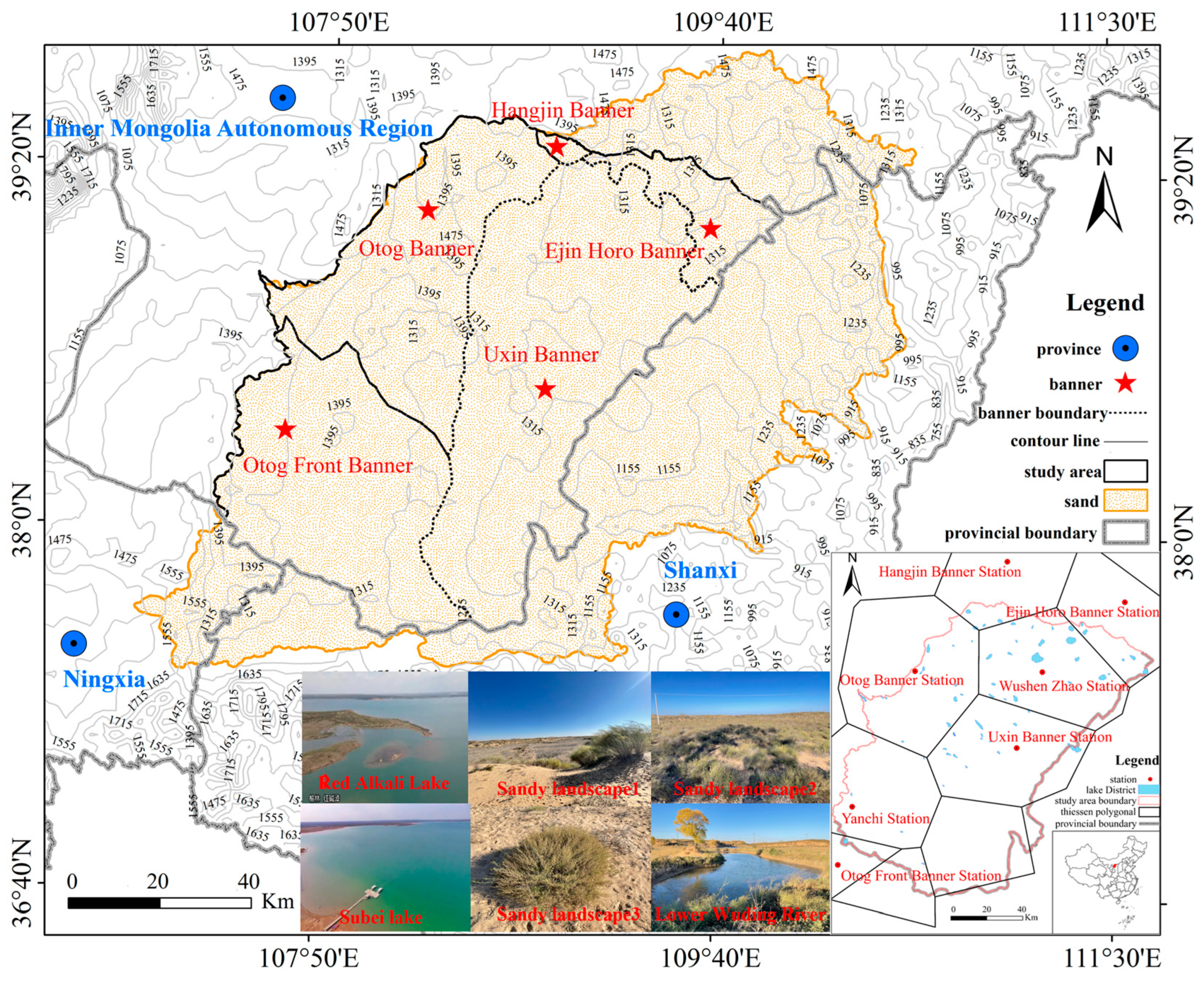
Figure 1. Study area (shown by black border) and Tyson polygon delineating the lake complex. Note: The study area is divided according to the distribution of meteorological stations using Tyson polygons into ETKQ, ETKQQ, HJQ, WSQ, WSZ, YC and YJHLQ.
Remotesensing 15 04153 g001
Figure 2. Number of years and months of landsat images available in the study area.
Remotesensing 15 04153 g002
Figure 3. Machine learning model workflow.
Remotesensing 15 04153 g003
Figure 4. Validation of GEE extraction of lakes.
Remotesensing 15 04153 g004
Figure 5. Changes in average lake area in the northwestern part of the Mu Us Sandy Land (2000–2020) are depicted in the image. Blue pixels represent shrinking lakes, while red pixels represent expanding lakes.
Remotesensing 15 04153 g005
Figure 6. Changes in the lake area in the Mu Us Sandy Land from 2000 to 2020.
Remotesensing 15 04153 g006
Figure 7. Correlation between 1-, 3-, 6-, 9-, and 12-month time scale SPEI and monthly scale lake area.
Remotesensing 15 04153 g007
Figure 8. Evaluation of the accuracy of the best prediction model for the Mu Us Sandy Land (best model names for MLSPEI-12 and MLSPEI-9 are in parentheses).
Remotesensing 15 04153 g008
Figure 9. Seasonal evaluation of relative error (the mean and Min-Max) of MLSPEI-9 and MLSPEI-12 in Mu Us Sandy Land (95% confidence intervals).
Remotesensing 15 04153 g009
Figure 10. Groundwater depth and lake area, February–September 2021.
Remotesensing 15 04153 g010
Table 1. Description of machine learning model parameters.
ReferenceNameDescription
Shrestha et al.
(2021) [21]
NBDefault
Khazaee et al.
(2019) [22]
KNNDefault
Koranga et al.
(2022) [23]
GBDTrandom_state = 2022,
max_depth = 4,
n_estimators = 200
Maier et al.
(2019) [24]
ExtraTreesrandom_state = 2022,
max_depth = 6,
n_estimators = 100
Chen et al.
(2022) [25]
RFrandom_state = 2022,
max_depth = 6,
n_estimators = 100
Ahirwal et al.
(2021) [26]
ABrandom_state = 2022
Ngo et al.
(2022) [27]
Baggingrandom_state = 2022
Ma et al.
(2021) [28]
XGBrandom_state = 2022,
max_depth = 6,
n_estimators = 200,
learning_rate = 0.3
Table 2. Lake size distribution in the Mu Us Sandy Land.
Lake Area (km2)Percentage
0.8–239.68
2–422.22
4–1025.40
>1012.70
Table 3. Percentage change in lake area in the northern part of the Mu Us Sandy Land, 2000–2020.
%Change in Mu Us DesertStudy Area
ETKQQETKQHJQWSQWSZYCYJHLQ
<2025604550502590
20–402020101525305
40–60151515205305
60–100105255550
>10030051015100
Disclaimer/Publisher’s Note: The statements, opinions and data contained in all publications are solely those of the individual author(s) and contributor(s) and not of MDPI and/or the editor(s). MDPI and/or the editor(s) disclaim responsibility for any injury to people or property resulting from any ideas, methods, instructions or products referred to in the content.