Article

Quantitative Characterization of Coastal Cliff Retreat and Landslide Processes at Portonovo–Trave Cliffs (Conero, Ancona, Italy) Using Multi-Source Remote Sensing Data

1
Department of Physics and Earth Sciences, University of Ferrara, 44122 Ferrara, Italy
2
Department of Biological, Geological and Environmental Sciences, Alma Mater Studiorum—University of Bologna, 40126 Bologna, Italy
3
Department of Pure and Applied Sciences, University of Urbino, 61029 Urbino, Italy
*
Author to whom correspondence should be addressed.
Remote Sens. 2023, 15(17), 4120; https://doi.org/10.3390/rs15174120
Submission received: 30 May 2023 / Revised: 24 July 2023 / Accepted: 18 August 2023 / Published: 22 August 2023
(This article belongs to the Special Issue Geological Applications of Remote Sensing and Photogrammetry)

Abstract

:
The integration of multiple data sources, including satellite imagery, aerial photography, and ground-based measurements, represents an important development in the study of landslide processes. The combination of different data sources can be very important in improving our understanding of geological phenomena, especially in cases of inaccessible areas. In this context, the study of coastal areas represents a real challenge for the research community, both for the inaccessibility of coastal slopes and for the numerous drivers that can control coastal processes (subaerial, marine, or endogenic). In this work, we present a case study of the Conero Regional Park (Northern Adriatic Sea, Ancona, Italy) cliff-top retreat, characterized by Neogenic soft rocks (flysch, molasse). In particular, the study is focused in the area between the beach of Portonovo and Trave (south of Ancona), which has been studied using aerial orthophoto acquired between 1978 and 2021, Unmanned Aerial Vehicle (UAV) photographs (and extracted photogrammetric model) surveyed in September 2021 and 2012 LiDAR data. Aerial orthophotos were analyzed through the United States Geological Survey’s (USGS) tool Digital Shoreline Analysis System (DSAS) to identify and estimate the top-cliff erosion. The results were supported by the analysis of wave data and rainfall from the correspondent period. It has been found that for the northernmost sector (Trave), in the examined period of 40 years, an erosion up to 40 m occurred. Furthermore, a Digital Elevation Model (DEM) of Difference (DoD) between a 2012 Digital Terrain Model (DTM) and a UAV Digital Surface Model (DSM) was implemented to corroborate the DSAS results, revealing a good agreement between the retreat areas, identified by DSAS, and the section of coast characterized by a high value of DoD.

1. Introduction

High coasts represent about 75% of the world’s coastline [1] and can be composed by both soft and hard rocks, with soft rocks usually characterized by an uniaxial compressive strength (UCS) ≤ 5 MPa, and hard rocks by UCS > 5 MPa [2].
The study of cliffed areas, with a particular focus on coastal retreats and slope failures, involves several factors such as geological, geomorphological, and structural settings [3,4], wave action [2,3,5,6,7,8,9,10], sediment input [11,12], cliff topography [13,14], beach width [15], and energy contents of waves [16].
In particular, geological structures can play a key role in controlling the morphology and stability of high coastlines [17,18], changing asymmetrically the values of shear strength and uniaxial compressive strength along the cliff. Furthermore, wave action and sea-level rise can lead to the creation of coastal notches and progressively to the collapse of large parts of the cliffs [2,19].
In this already complex scenario, the effect of climate change must be considered, which tends to modify the frequency and intensity of instability factors such as storminess, storm energy, and sea-level rise. In fact, although the role of such phenomena is well-known in coastal failures and retreats (even in case of single major events, Brooks and Spencer, 2016) [20], their prediction is becoming more and more difficult [21]. Examples of the effect of sea-level rise in coastal areas have been presented by Bruun 1962 [22] and Ashton et al., 2011 [23]. Diversely, from the model proposed by Bruun [22] for the sandy coast, Ashton et al. [23] demonstrated how, in the case of a high rocky coastline, the rate of sea-level rise results in an increased profile of slopes.
In the last decades, along with these new environmental challenges, new technologies have been developed and adapted for more accurate analysis. In particular, for cliffs, Terrestrial Laser Scanning (TLS) [24,25,26,27], orthophotos [28,29], UAV [30,31,32,33,34], and Persistent Scatterer Interferometry Synthetic Aperture Radar (PSInSAR) [35] were successfully used for monitoring their temporal and morphometric evolution.
The use of aerial photographs can be very useful for the assessment and evolution of cliff behavior along wide coastal sections. However, the spatial and temporal resolution of aerial photographs is often not suitable to gather significant results [28]. The adoption of more recent survey techniques (when available) for reconstructing coastal topography, such as Aiborne and Terrestrial Laser Scanning (ALS/TLS) and UAV, remarkably improve the evaluation of short- to medium-term cliff-erosion processes and rates [7,31,36,37]. TLS is very accurate, but it may be difficult to use in coastal areas because of the inaccessibility of many slopes. The use of ALS overcomes the problem connected with the TLS. However, it may be very expensive. As for the TLS and ALS, the UAV can be used to derive DEMs of the investigated areas. Although, there is a lower accuracy of the products [38,39,40,41], they represent a low-cost solution to acquire data at a local and large scale, as well as in inaccessible areas, constituting one of the best cost-effective choices in coastal monitoring [42]. In some cases, the combination of the above-mentioned techniques become very important (although challenging) to obtain a more complete dataset (in terms of spatial and temporal data) [28,32,33,43,44].
In this context, this paper aims to study erosion processes in the area between Portonovo and Trave (Ancona, Italy, Figure 1) through the combined use of aerial photography, UAV photogrammetry, and LiDAR data. It is important to note that these remote-sensing techniques played an outstanding role, providing the possibility to study the entire area, decreasing the risk for surveyor. The integration of these remote-sensing techniques with conventional geological and geomorphological surveys allowed for the recognition of the coastline sectors with higher retreat values and, at the same time, the exploration of potential and more important factors contributing to the retreat. In particular, we have considered geological, geomorphological, structural, meteorological, and marine factors.
The cliff top retreat analysis has been carried out through the Digital Shoreline Analysis System (DSAS) [45] and DoD calculations. The DSAS was applied to orthophotos spanning from 1978 to 2021. A DSM of the area was created from a UAV survey conducted in 2021 and compared with 2012 LiDAR data DTM for the DoD calculations.

2. Study Area Description

The study area is located in the central Adriatic coast, a few kilometers south of Ancona, between Portonovo and Trave in the Conero promontory (Figure 1). This area is characterized by high cliffs ranging from tens to hundred of meters in elevation and slopes from almost flat to 80° of steepness.
From a geological point of view, the Conero promontory belongs to the central sector of the present-day foredeep basin and foreland ramp of the Outer Northern Apennine fold and thrust belt [46,47,48,49]. In the study area, Neogenic formations from Miocene present time outcrops. These formations, Schlier, Formazione a Colombacci, Formazione di Sapigno, Orizzonte del Trave, and Argille Azzurre [50], are mainly composed by marls, clays, sandstones, and gypsum. The bedrock is often covered by landslide deposits, which are well-recognizable along the whole study area [51].
The structural setting of the area is characterized by the presence of two principal thrusts with typical Apennine lineaments NW–SE oriented, which are well-known in the literature [50]. The first one is well-exposed between Portonovo and Mezzavalle, and brings the Schlier Fm. on top of the Colombacci Fm.; the second thrust, close to the Trave, brings the Sapigno Fm. over the Argille Azzurre Fm.
From the geomorphological viewpoint, intense processes of erosion and many landslides characterize this part/sector of the coastline, resulting in a badland-like appearance to these slopes.
The landslides are well-documented in the landslide database of Istituto Superiore per la Ricerca e Protezione Ambientale (ISPRA) IdroGEO, occurring mostly in the Trave sector (https://idrogeo.isprambiente.it/app/iffi/ (accessed on 24 July 2023)). The study area is characterized by composite landslides, rock rotational slides, clay/silt rotational slides, rock fall, rock block topple, and earthflow [52]. Landslides identified in the study area are active or re-activated the state of activity [53].
Their crown is prevalently located along the morphological edge that separates the inland from the coast. The area affected by landslide phenomena is estimated to be approximately 280,000 m2.
With regard to the pedology and soil cover, these have been documented and described by the Parco Nazionale del Conero authority (https://www.regione.marche.it/natura2000/public/allegati_blog/1682/File%20non%20disponibile.pdf (accessed on 24 July 2023)). The soil covering the marls and calcareous bedrock is called regosoil, or lithosoil Xerorthents typic and lithic. Unfortunatey, no information was reported about the different depth of this level along the coastline.
Further available data from Corine Land Cover (https://land.copernicus.eu/pan-european/corine-land-cover (accessed on 24 July 2023)) of 1990 and 2018 were checked in order to find information regarding land-use change and vegetation.
It has been determined that the area corresponding to the Trave sector was classified from 1990 with Code 141 as “green urban areas”, and the other wo sectors with the code 311 as “broad-leaved forest”. From 2018, the Trave sector was classified with Code 323 “sclerophyllous vegetation”, while the other two sectors remained under Code 311 as “broad-leaved forest”.
According to morphology and geological characteristics, the coastline has been divided in three different sectors (Figure 2) defined from South to North:
(a)
Sector “1”, named Portonovo, is E–O/NW–SE-oriented and stretches from Portonovo to the beginning of the Mezzavalle sector. This sector is mainly characterized by the Schlier Fm.
(b)
Sector “2”, called Mezzavalle, is approximately NW–SE-oriented and mainly covered by landslide deposits.
(c)
Sector “3”, entitled Trave, approximately N–S/NW–SE-oriented, is characterized by high and steep cliffs (±200 m), along which tectonized flyschoid formations (Argille Azzurre Fm.) outcrop.
Figure 2. Geological setting of the study area [50] and “Sectors”: (1) Portonovo; (2) Mezzavalle; (3) Trave. Bedrock legend: SAA (Scaglia Rossa Fm., Upper Cretaceous–Medium Eocene); VAS (Scaglia Variegata Fm., Medium Eocene–Upper Eocene), SCC (Scaglia Cinerea Fm., Upper Eocene–Upper Oligocene), BIS (Bisciaro Fm., Lower Miocene), SCH (Schlier Fm., Lower Miocene–Upper Miocene), GNOa (Sapigno Fm. Upper Miocene), FCO (Colombacci Fm., Upper Miocene), Tv (Trave horizon, Lower Pliocene), FAA (Argille Azzurre Fm., Lower Pliocene–Lower Pleistocene). The Trave horizon is a natural stratum that forms a ridge outcropping from the sea in the northern section of the study area.
Remotesensing 15 04120 g002
The coastline object of this study overlooks on the northern–central Adriatic Sea [54]. The Adriatic sea is a microtidal environment [54]; this sector is characterized by two different prevalent seas, with the reigning sea coming from S–SE (Sirocco), namely the most frequent direction of wave storm events and conjoined winds and dominant sea from NE (Bora), along the direction of wave storm with major intensity [55,56]. Additionally, it is possible to identify along the coast of this region a littoral drift moving northwards [57].

3. Materials and Methods

With the aim of quantifying morphodynamical processes acting on these cliffs, we have performed an interdisciplinary study, which includes:
(a)
Fieldwork.
(b)
The analysis of meteorological and marine data.
(c)
Cliff-top retreat in different periods, using the DSAS tool for ArcGis. (https://www.arcgis.com/home/index.html (accessed on 24 July 2023)).
(d)
DoD between an available 2012 Lidar data and a 2021 DSM extracted from UAV photographs to improve our understanding of cliff-retreat rate and validate results from multitemporal orthoimages analysis.

3.1. Fieldwork and GIS Topographic Analysis

During the fieldwork, a geological survey of the area was performed with the goal of improving the details of the existing maps/information integrated through the use of a pocket penetrometer and a Schmidt hammer according with ISRM guidelines [58]. This allowed for the values of uniaxial compressive strength (UCS) to be gathered, both for deposits and bedrock in the three studied sectors. Furthermore, to improve the information about rock mass quality along the coastline, the rock mass classification “geological strength index” (GSI) was performed [59,60,61,62,63]. Starting from the 2012 DTM provided by Marche region in GIS environment, an elevation model was conducted, including the symbology of the raster, and a slope model was created with the tool slope.
Furthermore, the beach width in the different sectors was extracted in GIS, starting from an orthophoto recorded on 28/29 September, 2021. Profiles spaced 30 m, for a total of 104, were traced perpendicularly with respect to the shoreline and width measured along their length between the berm crest and the cliff base. Then, all the values obtained were stored in a table, and a mean value for each sector was identified.

3.2. Analysis of Meteo and Marine Data

The analysis of marine data was implemented using the 1994–2019 wave hindcast produced by CNR–ISMAR for the Adriatic Sea in the framework of a collaboration between the University of Ferrara, the CNR–ISMAR, and the Autorità di Bacino del Fiume Po (ADBPO). This was part of the Research Programme Venezia 2021, coordinated by CORILA, with the contribution of the Provveditorato for the Public Works of Veneto, Trentino Alto Adige, and Friuli Venezia Giulia [64]. The wave dataset is based on the WaveWatch3 (WW3) numerical model implemented for the Adriatic Sea using a grid with spatial resolution ~2.5 km using high resolution (~80 m) bathymetry from EMODnet. The model was forced with an edited version of ERA5 to correct the bias due to the general underestimation of the wind intensity on the Mediterranean Sea of the original dataset. The wave dataset is provided in NETCDF format (i.e., one file for each year, hourly data). The 2018 high-resolution bathymetry from ARPAE was used to extract the 20-m depth bathymetric contour as source to extract coastal points as reference positions for the analysis. A set of coastal points was defined in front of the Mezzavalle–Trave area (Figure 3).
The significant wave-height (Hs) timeseries was extracted from the gridded data of the CNR–ISMAR datasets for each defined coastal point using the nearest point method. The yearly timeseries were merged. Independent extremes were identified through a peak-over-threshold analysis, where the threshold was calculated as a quantile of the provided timeseries, and the independence criteria were based on a time window.
The analysis was implemented using the python library pyextremes (https://georgebv.github.io/pyextremes/ (accessed on 24 July 2023)).
Regarding the rainfall data, these were retrieved from Sistema Informativo Regionale Protezione Civile Marche. The data are available on Regione Marche website (https://www.regione.marche.it/Regione-Utile/Protezione-Civile/Progetti-e-Pubblicazioni/Annali-Idrologici#Annali-Idrologici---Parte-1 (accessed on 24 July 2023)) from 1990 and are related to the meteorological station “Ancona Torrette” with a daily sample frequency and without gaps. From 2003, another station was used, “Ancona Regione RT-1638;” data are available in the website after registration (http://app.protezionecivile.marche.it/sol/indexjs.sol?lang=it (accessed on 24 July 2023)) with a sample frequency of 15 min and no gaps in the record. Both stations are ca 5–8 km north from the cliffs object of this study.

3.3. UAV Survey and Data Elaboration

Due to the extension of the study area (about 1.5 km2), the UAV data acquisition was accomplished in two consecutive days, 28/29 September, 2021, using a commercial drone DJI Phantom Vision 3+ Pro equipped with a camera: FC300X (focal length: 3.61 mm; pixel size: 1.56 μm × 1.56 μm).
Flights were conducted at a constant elevation of 120 m covering the top cliff, and 60–70 m covering the beach area, using automated flight plans created using the “Drone deploy” opensource application (https://www.dronedeploy.com/ (accessed on 24 July 2023)). Front and side overlap between each photo was ~70%, and flight speed was 8–10 m/s.
The UAV survey was supported by an RTK–GNSS survey using a Trimble RTK–DGPS R8 (i.e., stop-and-go technique; horizontal accuracy of 8 mm and vertical accuracy of 15 mm), which was used to acquire the position of 22 ground control points (GCPs). These were made of white-and-red wooden square targets, measuring 60 cm × 60 cm, and distributed within the study area. The Universal Transversal Mercatore WGS84 zone 33N was used as coordinate system, and the ellipsoidal height was converted to orthometric height using national grids using the software “Convergo” version 2.05 (https://www.cisis.it/?page_id=3214 (accessed on 24 July 2023)). Estimate error during the RTK–GNSS survey was approximately 6 cm horizontally and vertically.
“Agisoft Metashape” (version 1.5.1 https://www.agisoft.com (accessed on 24 July 2023)) was used to manage and process UAV data and GCP coordinates. Using the procedure suggested by different authors [41,65,66,67,68], it was possible to create the DSM and orthophoto of the surveyed area.

3.4. Morphological Analysis

Although the DSAS tool was created to analyze the shoreline movements, its use in cliff-retreat studies is widely documented in the literature [69,70,71,72].
The study was performed using orthophoto acquired in 1978, 1998, 2007, 2010, and 2021. The first four (1978, 1998, 2007, and 2010) are available on institutional websites (http://www.pcn.minambiente.it/viewer/index.php (accessed on 24 July 2023), http://wms.cartografia.marche.it/geoserver/Ortofoto/wms (accessed on 24 July 2023)). The 2021 orthophoto is the one extracted from UAV photographs. Spatial resolutions of such orthophotos are reported in Table 1.
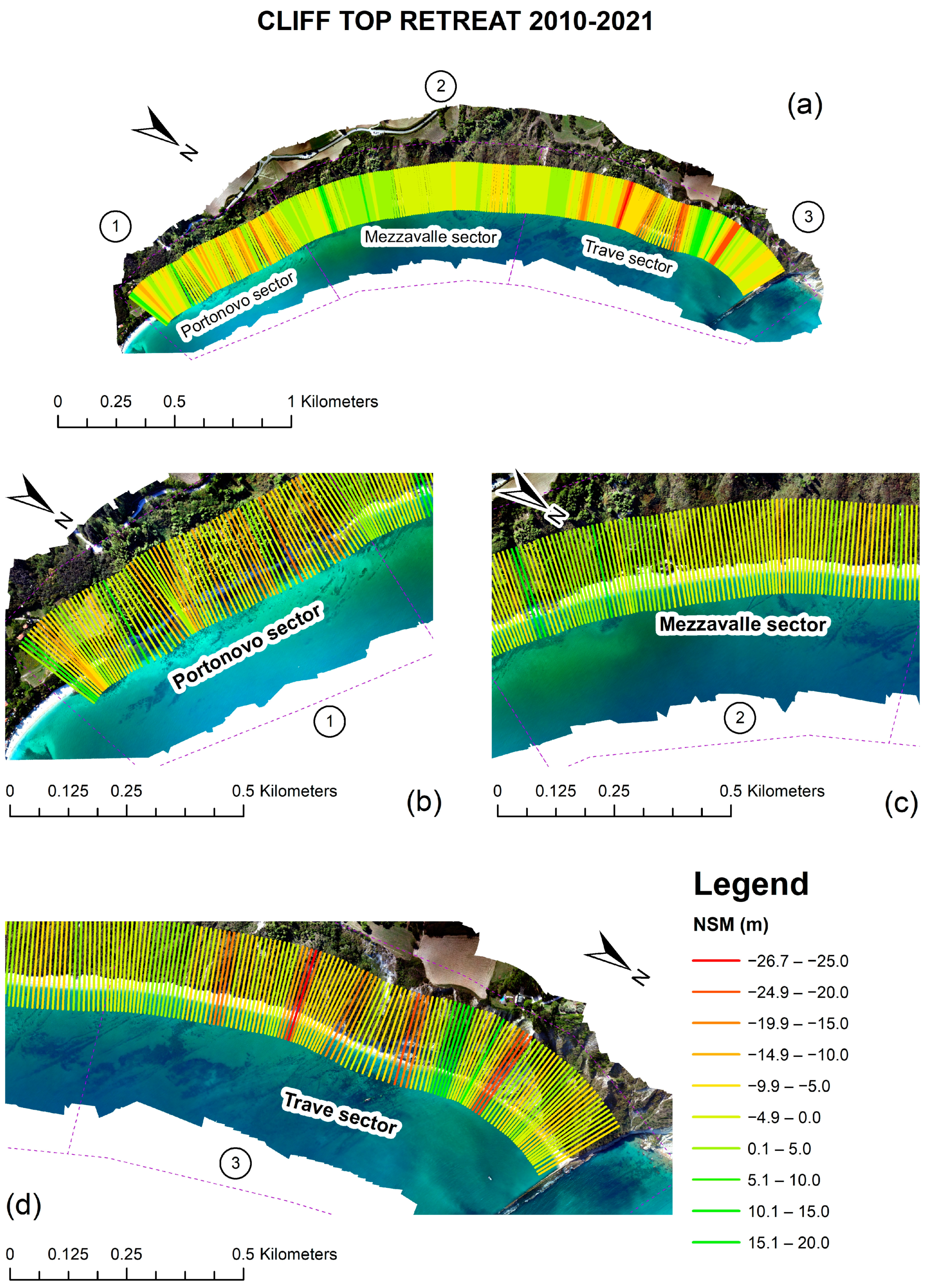
The DSAS analysis is based on the comparison of different cliff top edges mapped over the years. The comparison is made using the cliff tops edges and a baseline as reference line. Cliff top edges were manually mapped on the orthophotos, keeping the same visual scale on all the photos (Scale 1:3000) and using the limit between vegetation and bare slope as edge of the cliff (Figure 4a). The accuracy of manual mapping was defined following the example of Crowell et al. (1991), Fletcher et al. (2003), and Del Río and Gracia (2013) [73,74,75]. The approach used is based on the use of the Spatial Adjustment tool in ArcGIS [67,76,77,78]; the cliff top edge is mapped four different times, and the difference between each line is then calculated measuring the offset between a couple of lines per time along several perpendicular thick profiles. Once each couple of the dataset (for each image) was tested, the highest error was used as reference. For what concerns DSAS calculations, as reference line and base line, we have used the shoreline, which was mapped in the 2021 orthophoto, thanks to the different colors between the sand and the sea. The same procedure described before was used to calculate the error in the digitalization of the shoreline. Hence, a 100-m buffer of this line was used in GIS environment (while ensuring that the buffer was beyond the cliff top edges) (Figure 4b). Starting from this baseline, the software creates a series of transects. In this case, we have defined a distance between each transects of 10 m for a total of 310 transects. An example of transects created during the DSAS analysis is shown in Figure 4c. Among them, the software verifies the changes in the cliff top edges and calculates the Net Shoreline Movement (NSM, the total movement measured in meters) and the End Point Rate (EPR, the rate of movement calculated in meters per years). Hence, Confidence of End Point Rate (ECI or EPRunc in newer versions of DSAS) was calculated. This is an index that considers the uncertainty of lines (accuracy error) as a factor for calculating the EPR confidence.
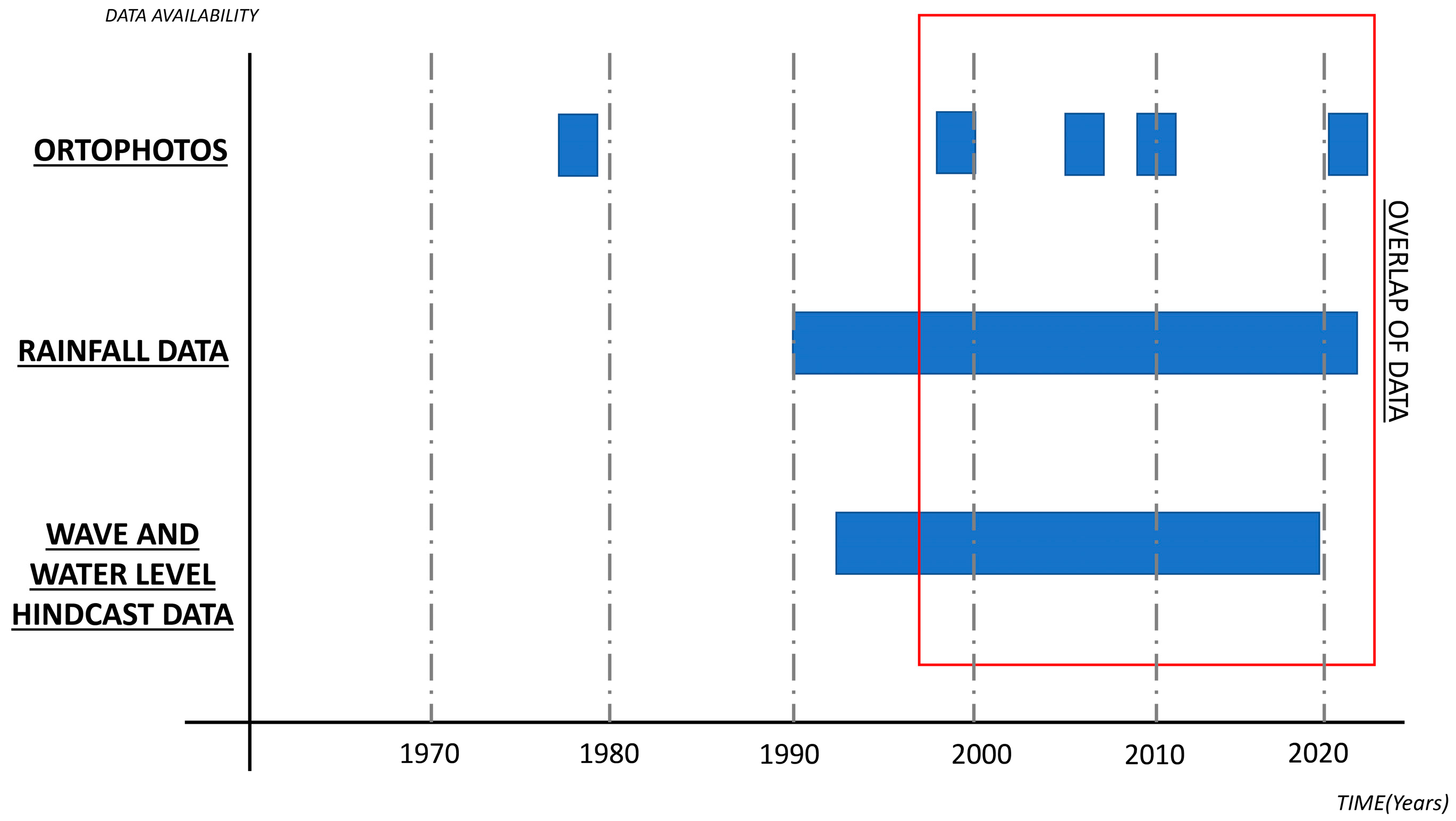
Considering the available information about waves (1994–2019) and precipitation (1990 to current), it was decided to perform DSAS analysis using time spans 1998–2007 and 2010–2021 in order to have a temporal correspondence between computed erosion processes and external drives (Figure 5). A further analysis was also undertaken for the period 1978–2021 (although no wave and precipitation were available until 1990) to verify the coastal retreat in the whole 40 years and compare such results with other periods.
Finally, to further verify the results of DSAS analysis, a DoD analysis was conducted. The use of DoD is becoming a common practice in geosciences [70,79,80]. In this case, we have used the 2012 airborne Lidar (near infrared and green) DTM with a cell size of 4 m × 4 m provided by Marche Region, and the 2021 UAV extracted DSM with a cell size of 0.25 m × 0.25 m. The accuracy of UAV-extracted DSM product was computed, verifying the differences between control points coordinates acquired through RTK–DGPS and the coordinates of same points on UAV-extracted DSM while computing the mean error and the RMSE. In particular, we have found a planimetric mean error of 31 cm with RMSE of 12 cm and a vertical mean error of 5 cm with a RMSE of 6 cm [81]. The 2012 airborne Lidar has a vertical RMSE < 10 cm and a planimetric RMSE < 10 cm, as reported by the Marche Region. The two rasters were compared after a resample, keeping the coarsest resolution through the GIS tools resample and clip. Vegetated areas were excluded from the analysis, and the UAV DSM was resampled at the same resolution of the Lidar-based DTM. The raster calculator was used to compute the differences between the two rasters in elevation. Statistical analysis on resulting data was performed for each sector, obtaining mean, maximum, and minimum values of variation for each sector.

4. Results

4.1. Fieldwork and GIS Analysis

The geological and structural surveys highlighted the main differences between the three sectors.
Moving from Portonovo to Trave, we found different geological formations, i.e., Schlier Fm./Sapigno Fm./Argille Azzurre Fm., and Colombacci Fm. with different geotechnical characteristics, as evidenced by the values of GSI and UCS gathered through a pocket penetrometer and a Schmidt hammer (Table 2). Rock-mass classification, together with UCS, has been shown to be a factor of unneglectable importance in coastal-cliff erosion, predisposing slopes to more frequent failures [2,8,82]. Therefore, we have considered that GSI and UCS represent the more suitable geotechnical parameters to characterize, according to the lithotypes outcropping in the area, soil or weak rocks.
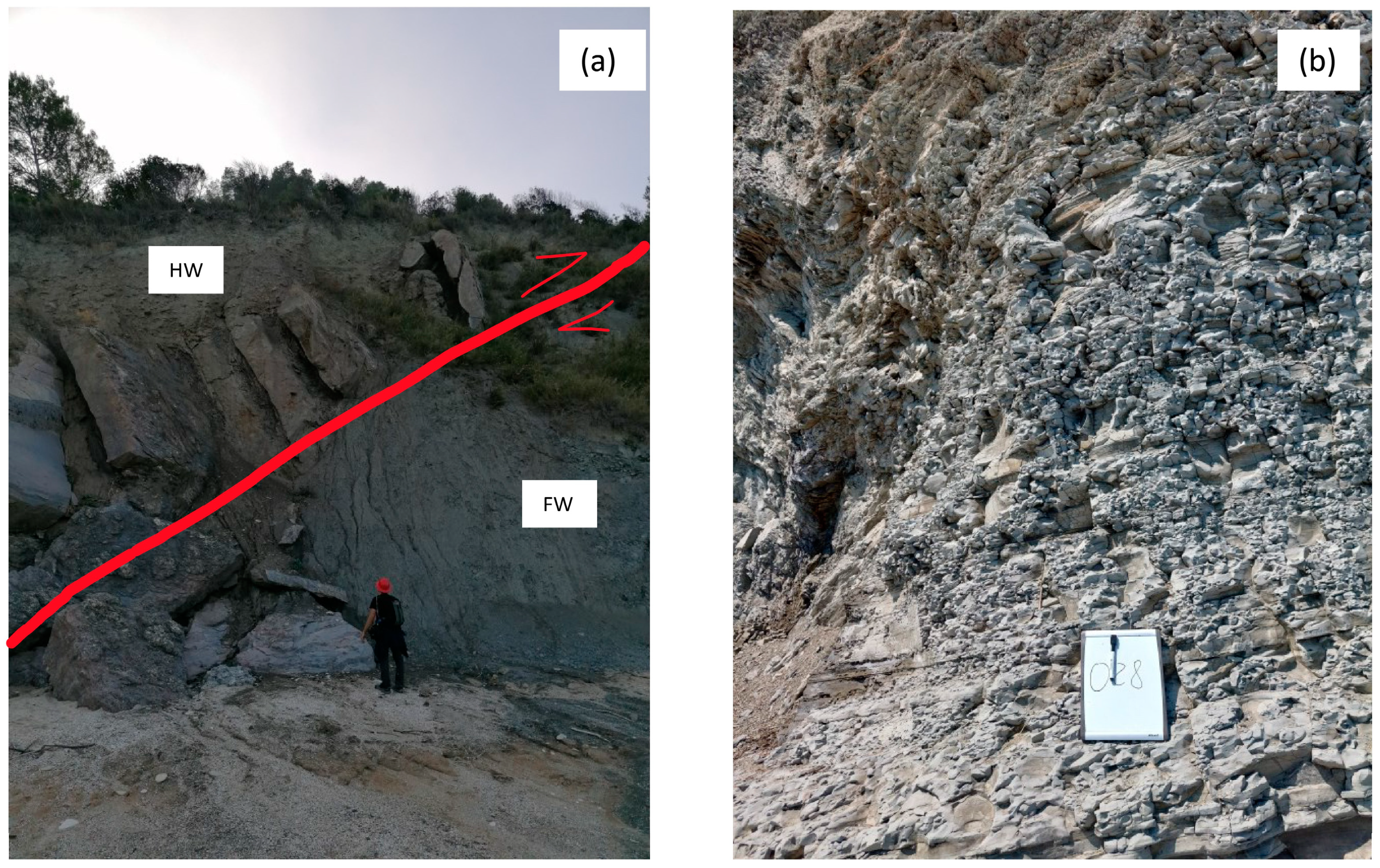
We obtained the smallest values of UCS along the Mezzavalle sector, which is basically characterized by landslide deposits (for them, the GSI classification is not applicable). In the Portonovo sector, we obtained the highest values of GSI and UCS. In the Trave sector, these values are very variable and depend on the structural features present, which determine a high fracturing degree, as in corresponding to the tectonic contact between the Sapigno Fm. and the Argille Azzurre Fm. (Figure 6a), which gave rise to a completely fractured zone in the Argille Azzurre Fm. itself (Figure 6b).
Furthermore, thematic maps developed in GIS using LiDAR data show that, among the three sectors, the Trave sector is characterized by the steepest and highest cliffs (Figure 7). The mean beach width computed of the three sectors was 6.7 m, 23.5 m, and 7.6 m for Portonovo, Mezzavalle, and Trave, respectively.

4.2. Analysis of Meteo and Marine Data

Data from CNR–ISMAR are displayed in Figure 8, along with the results of the POT analysis (threshold: 99.5 percentile; independence criteria: 48 h) for the significant wave height (hs) for the coastal point CP005. Here, the hindcasted over-threshold events between 1994 and 2019 are reported. The average number of events per year is 4.5, which is in line with the expected range (3–5) for traditional POT analysis. It is not possible to identify any kind of trend in the rate of storminess in the whole period considered; it can be only noted that after 2012, the number of events with Hs > 4.5 m is higher in respect to the period before (1994–2012).
Regarding the rainfall data, the annual average precipitation recorded between 1990 and 2021 is 664 mm. It is possible to identify two years where precipitation exceeded mean values, 2010 (with 1034 mm) and 2014 (with 966 mm), and two years with dryer conditions, 2011 and 2012, with 433 mm and 447 mm of precipitation, respectively (Figure 8).

4.3. Morphological Analysis

Digitalization of the cliff top and the shoreline has been performed, and the maximum Root Mean Square Error (RMSE) of this operation was calculated. In particular, it has been found that the maximum RMSE for cliff top digitalization was obtained for the 1978 ortophoto, with a value of 3.89 m. Shoreline digitalization was performed on the 2021 orthophoto and resulted in a RMSE of 0.85 m.
Considering the whole period 1978–2021 (Figure 9), the Trave sector is the portion with the highest mean value of EPR; the Portonovo sector shows a similar behavior; and the Mezzavalle sector shows a marginally positive value. Moreover, focusing on specific area within each sector, values of almost −1 m/yr of EPR are reached between transects 21–31 and 251–291 in Portonovo and Trave sector, respectively. The ECI computed for this time span is 0.16 m.
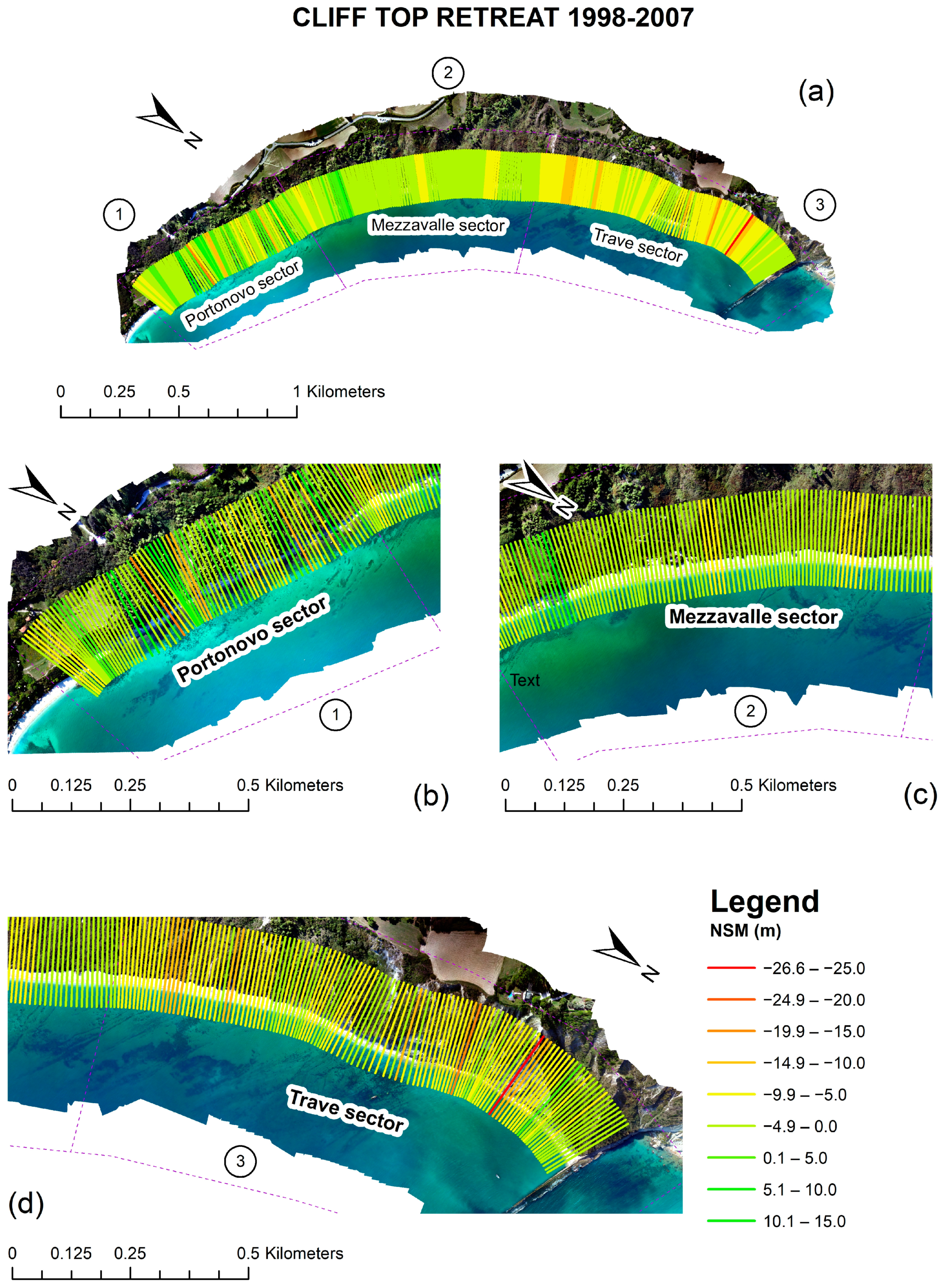
Furthermore, the analysis shows that in the period from 1998–2007 (Figure 10), the cliff top retreat was more concentrated in the Trave sector, where we calculated an average mean EPR three times higher than the value obtained for Portonovo and Mezzavalle sectors in the same period. The highest values of EPR were recorded between transects 26 and 44 in the Portonovo sector, with values around −2 m/yr and between transects 266 and 286 in the Trave sector where we reached the value of −3 m/yr in the EPR. ECI in this time span is 0.79 m.
During the period from 2010–2021 (Figure 11), the Trave sector resulted in the highest negative values of EPR, which was very similar to the Portonovo sector and four times higher than in the Mezzavalle sector.
Between Transects 226–236 (Trave sector), the EPR overcame −2 m/yr. The ECI for this period is 0.62 m. All the values regarding the mean EPR and ECI are illustrated in Table 3, while NSM values are represented in Figure 9, Figure 10 and Figure 11.
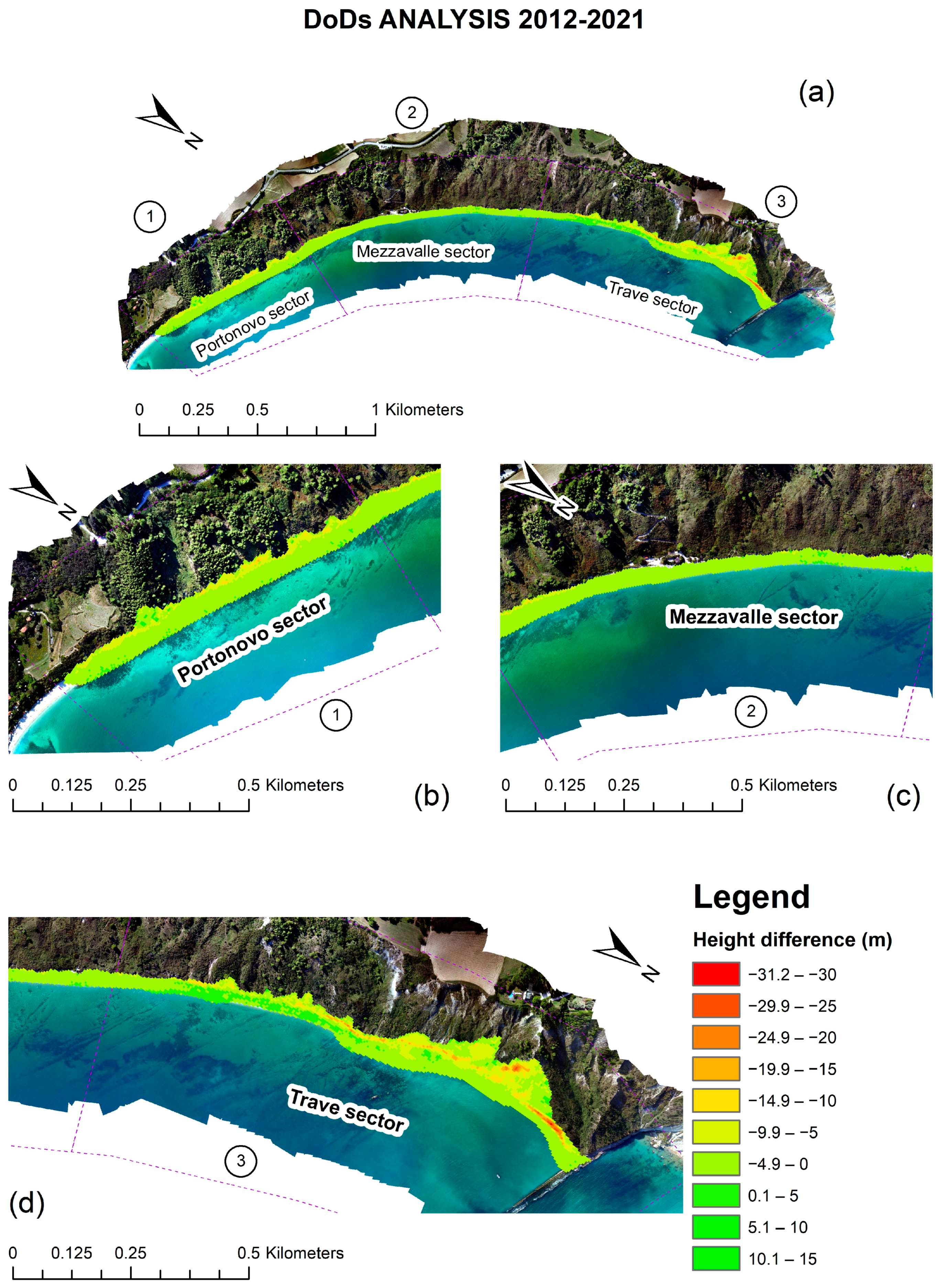
For what concerns the DoD analysis (Figure 12), the Portonovo sector presents a negative mean value of variation from 2012 to 2021 of −2.2 m in elevation. The highest negative value recorded was −16.3 m between transects 51–57 in the middle part of the Portonovo sector, where landslides deposits currently overlay the bedrock.
The DoDs analysis allows for the comparison of the 2012 DTM and the 2021 DSM, and it highlights difference in elevation between this period. Negative values indicate the loss of material, while positive values indicate accumulation. The Mezzavalle sector displays negative mean values of DoDs of −1.4 m, while the maximum height difference is −12.6 m in the southern part of the area, between Transects 87–94, where Schlier Fm. outcrops. In the rest of the sector, no other clear difference was recorded except for a single pixel value that shows increase for 6.4 m and associated probably with the presence of vegetation (Figure 12). In the Trave sector, a negative mean variation of −3.7 m was recorded for the whole area, with the highest value of −31.2 m between Transects 289–301 near Trave rock. Other negative height differences greater than −10 m were recorded close to the edge of cliff top, from Transect 230 to 282. Evident areas characterized by positive (accumulation) values were not found. This is probably related to sea action, which tends to remove landslide deposits.
The uncertainty of the DoD was computed, propagating the uncertainty of the input DEMs by applying the root of the sum of the square [83] and obtaining values of 11.18 cm for z and 15.62 cm for the planimetric component. Furthermore, we refined this result, multiplying the error values for a t-value of 1.96 [41,84] and obtaining an uncertainty of 21.98 cm for z and 30.61 cm for planimetric component.

5. Discussion

Results from the DSAS analysis show how this coastline is geomorphologically an active area. The average retreat rate calculated in the period from 1978–2001 was −0.25 m/yr. More specifically, in the three sectors, we can summarize the following outcomes.
The Trave sector shows the highest rate of cliff retreat, in the period from 1998–2007, where the mean is −0.72 m/yr (almost three times higher than the average retreat calculate in the whole area). The Mezzavalle sector possesses the lowest retreat rate during all the time spans. Despite this, the latter sector is mainly characterized by landslide deposits with poor geotechnical properties, and it is well-known that geotechnical properties play a key role in cliff erosion/retreat [82]. The Portonovo sector shows an intermediate behavior between the other two sectors, more similar to Trave, exhibiting in the period from 2010–2021 a retreat rate doubled that of the entire period from 1978–2021. Many authors have drawn attention to the range of coastal cliff retreat [3,70,82,85], focusing especially on weak rocks, and obtaining average values of −0.25 m/yr [82]. Interestingly, while average retreats gathered by other authors are perfectly comparable with our values, the Trave sector shows values nearly three times higher than the mean value reported in GlobR2C2 [82]. Looking to other Italian case studies, we can see that in Punta Caleo headland (Campania region), a retreat of 15 m over 30 years was founded (0.5 m/yr). In the close locality of Torre la Punta (1 km far from Punta Caleo), a retreat rate of 0.8 m/yr was assessed, showing how the rate of erosion can suddenly vary in the same coastal areas [8]. Regarding other cases in the Adriatic Sea, in Torre dell’Orso (Apulia region), the rate of erosion (in fine limestones) was found to be between 0.08 m/yr and 0.12 m/yr [71,86], while in the Abruzzo region (on the Pleistocene clay–sand–sandstone–conglomerate marine sequence), the retreat rate ranged between 0.15 m/yr and 1 m/yr [87]. In the area between Gabicce and Pesaro, a few kilometers northward of our case study (characterized by similar lithologies), a mean retreat rate of 0.16 m/yr was calculated in the last 6000 year [88]. Considering the much smaller time span considered in our study, these values cannot be compared.
In relation to the above discussion, the information about precipitation, waves, geology, and land cover has been examined in order to understand the main factors controlling such erosion processes. Although a complete time overlap between precipitation and wave data is not present, the coverage is enough only in the 1998–2021 temporal window (Figure 5) to understand potential correlation between these factors and cliff retreat. It has been commented above that the highest rate of retreat has been measured in the Trave sector in the period from 1998–2007. Considering extreme events for precipitations and waves, respectively, the result is there is no correlation between the highest rate of cliff retreat measured in the period from 1998–2007 in the Trave sector and these two parameters. It is difficult with the available data to perfectly match cliff top retreat occurrence and singular meteo/marine events because orthophotos are yearly distributed, and even marine data are not completely reliable because they derive from an hindcast elaboration. Yet, performing an extreme-value analysis of marine data will be useless without the possibility to assess with photos the effect of waves on the slopes. The same issue is related to rainfall data. From September 2003, it is possible to have information on the precipitation every 15 min. However, the lack of data does not allow for a cause–consequence analysis that correlates the main raining events and landslide triggering. As numerous authors have demonstrated, a soft-rock cliff recession is an episodic and localized phenomenon [2]. For example, on 14 September, 1944, a storm on Long Island, New York, cut back a cliff made of glacial deposits by a horizontal distance of more than 12 m in a single day [89]. At Santa Cruz, during storms in January 1983, waves eroded around 14 m of the bluff top in Miocene mudstone–siltstone cliffs. Due to this, it is challenging to constrain which events and drives can have a greater impact on the cliffs without a complete dataset [90]. As a result, other parameters have to be used to understand possible correlations.
Other important features that have to be considered are: beach width, geotechnical properties, and slope-cliff elevation/steepness [15,82,91]
Regarding the beach width, it has been noted that the Mezzavalle sector has the widest beach, followed by the Portonovo and Trave sectors, which have almost the same beach width mean.
The sector with the highest geotechnical properties is the Portonovo sector, while the one with the lowest values is Mezzavalle (made prevalently by landslide deposits).
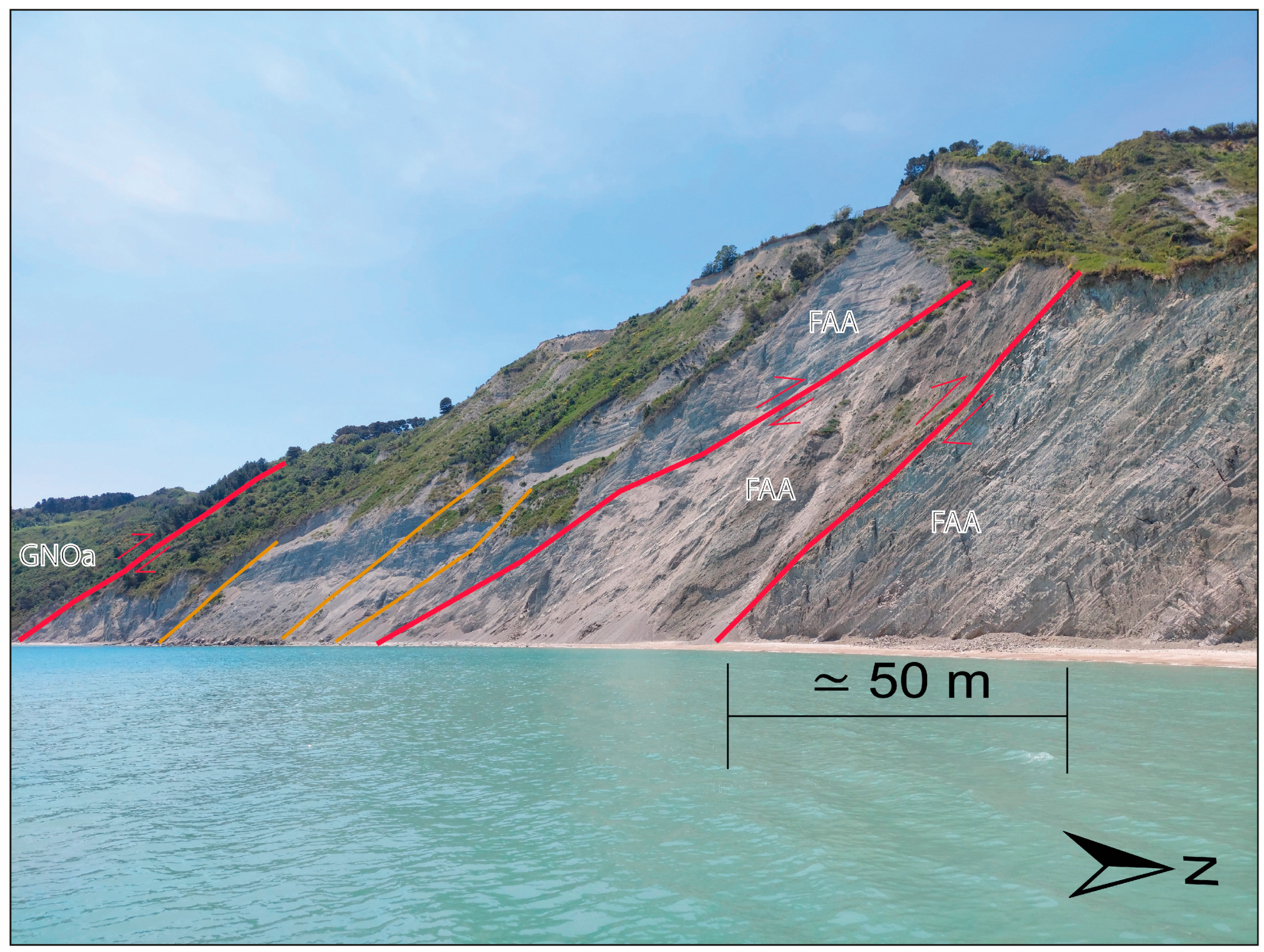
The geological survey shows that the Trave sector is the area most intersected by tectonic features, with two main thrusts present (Figure 13). Furthermore, the Trave sector is the one with highest cliff elevation and steepness. Clearly, such fractures decrease the geotechnical properties (lower values of GSI) of rock masses and their stability [6]. This is also confirmed by the landslide inventory of ISPRA, where most of the landslide documented occurred in the Trave sector (https://idrogeo.isprambiente.it/app/iffi/ (accessed on 24 July 2023).
Additionally, as observed on the California coast, fracture spacing plays a very important role in retreat rates [92,93].
Another important aspect to be discussed is related to the land cover of the study area. No information was reported about the different depths of soil covers along the coastline, but many considerations can be made. The fieldwork has observed that the landslide deposits outcropping in the Portonovo sector are more granular than those present in Mezzavalle (composed mainly by clays). This, combined with the higher steepness of the Portonovo and Trave sectors, results in the hypothesis that the soil cover depth in the Mezzavalle sector could be higher than the others sectors (pedogenesis is usually more prone to develop in the flatter area [94]). This can also be linked with the resulted higher occurrence of flow, like landslides, in the Mezzavalle sector, which was reported by IdroGEO in the areas behind the active cliffs.
Another issue to be discussed is related to the presence of vegetation in the three sectors. The analysis of UAV photographs highlighted that the Trave sector, compared with the other sectors, presents in the cliff top a lower vegetation rate and a different land cover (in agreement with Corine Land Cover, which defines the vegetation on that sector as sclerophyllous vegetation).
From a geomorphological point of view, this evidence can provide us more insight regarding the process acting on the cliff. In fact, it is possible to state that with a lower vegetation rate, run-off processes can be more severe, increasing the instability of the rock mass. These observations agree with what was showed by the DoDs analysis, where the sector with the major negative differences (loss of material) is Trave. Observing the shape and distribution of the area with higher DoD values, it is also possible to notice that these are mainly localized along the cliff top. This evidence, combined with the lack of evidence of detectable notches at the cliff base, leads us to think that the erosive process is more influenced by slope processes than marine forcing. Dods analysis showed that the Mezzavalle sector presents the lowest variation, while Portonovo is an intermediate behavior between the other two. This datum completely agrees with the results gathered from the DSAS analysis: area with a positive difference (accumulation) has a very minor width, which is probably related to the capacity of the sea to quickly remove slope-collapsed materials.
The integration of DSAS and DoDs analysis guarantee confirmed areas with major failures/erosions activity. These results confirm that the continuation of multitemporal survey can represent a good method in monitoring the evolution of this coastline.

6. Conclusions

This study represents the first attempt of quantifying morphodynamical processes acting on Portonovo–Mezzavalle–Trave cliffs.
An interdisciplinary study, which includes fieldwork, an analysis of meteorological and marine data, geological and land cover information, and cliff-top retreats in different periods, has been performed using the DSAS tool for ArcGis. Moreover, to improve our understanding of the cliff-retreat rate and validate results from the multitemporal orthoimages analysis, we performed a DoD between available 2012 DTM data and a 2021 DSM extracted from UAV photographs.
The results gathered from the study can be summarized as follows:
(a)
The coastal area that shows the highest variation in all the time spans considered is the Trave sector, showing an NSM maximum retreat of −43.5 m and a maximum height difference of −31 m.
(b)
Comparing different time periods, there is an augmented cliff-top erosion trend over the last 20 years if compared to the whole period of analysis (1978–2021).
(c)
The Trave sector shows values of retreat nearly three times higher than the mean value reported in GlobR2C2 [82].
We conclude that the higher retreat rate localized at the Trave sector is related to a combination of factors:
(a)
Mechanical properties of the rockmass are decreased due to the presence of tectonic disturbances, which increase fracture intensity and result in a decreasing GSI.
(b)
The steepness and elevation of this sector, which is the highest in the entire investigated coastline (both are landslide-predisposing factors).
(c)
One of the lowest values of beach width, which increases the role of wave action.
(d)
Variations of vegetation rate and land cover may affect the run-off and the erosion in the upper slope.
The situation at the Mezzavalle sector is different: it is characterized by the lowest values of geotechnical properties, the highest values of beach width, and by the value of elevation of the cliff, which is much lower than those in the Trave sector. The Mezzavalle sector is the area with the lowest rate of cliff retreat.
The Portonovo sector shows an intermediate behavior between the other two, more similar to the Trave sector.
Precipitations and waves data do not seem to have a correlation with the different erosional process in the different sectors. In fact, there is no correlation between years that have a high rate of precipitation and waves data, and the high rate of cliff retreat measured in the Trave sector between 1998–2007. From a geomorphological perspective, the data gathered in the study allows us to hypothesize that the evolution of this coastline is more controlled by slope factors than marine drives, leading to a progressive retrogression of the cliff-top edge.

Author Contributions

Conceptualization: N.F.; methodology N.F., M.F., S.F., E.D., M.G. and P.C.; validation, N.F., M.F., S.F., E.D., M.G. and P.C.; formal analysis: N.F., M.F., S.F., E.D., M.G. and P.C.; investigation: N.F., M.F., S.F. and E.D.; resources: M.G. and P.C.; data curation: N.F., E.D.; writing—original draft preparation: N.F.; writing—review and editing: N.F., M.F., S.F., E.D., M.G. and P.C.; supervision: M.F., S.F., E.D., M.G. and P.C.; project administration: M.G. and P.C.; funding acquisition: M.G. and P.C. All authors have read and agreed to the published version of the manuscript.

Funding

N.F. acknowledges the University of Ferrara for providing a fellowship within the EMAS PhD program. The wave database provided by ISMAR-CNR was developed within the Accordo Mare of ADBPO (Coordinator P. Ciavola) and by the project VE2021 financed by CORILA.

Data Availability Statement

Survey data can be requested to the authors after completion of N. Fullin PhD program. Wave data remains property of the funders.

Acknowledgments

The authors are grateful to the people that have supported the fieldwork and shared useful advises, in particular, Davide Torre, Angelo Ballaera, Alessia Sciati, Alberto Riva, and Marco Menichetti. Furthermore, we thank C. Ferrarin, A. Benettazzo and F. Barbariol for providing advice and wave data.

Conflicts of Interest

The authors declare no conflict of interest.

References

  1. Williams, A.; Pranzini, E. Rock Coasts. In Encyclopedia of Coastal Science; Shwartz, M.L., Ed.; Springer: Berlin/Heidelberg, Germany, 2018. [Google Scholar] [CrossRef]
  2. Sunamura, T. Rocky Coast Processes: With Special Reference to the Recession of Soft Rock Cliffs. Proc. Japan Acad. Ser. B Phys. Biol. Sci. 2015, 91, 481–500. [Google Scholar] [CrossRef]
  3. Tsuguo, S. Coastal morphology and research. In Geomorphology of Rocky Coasts; J. Wiley: Chichester, UK; New York, NY, USA, 1992; ISBN 0471917753. [Google Scholar]
  4. Trenhaile, A.S. Cliffs and Rock Coasts; Elsevier Inc.: Amsterdam, The Netherlands, 2012; Volume 3, ISBN 9780080878850. [Google Scholar]
  5. Naylor, L.A.; Stephenson, W.J.; Trenhaile, A.S. Rock Coast Geomorphology: Recent Advances and Future Research Directions. Geomorphology 2010, 114, 3–11. [Google Scholar] [CrossRef]
  6. Brideau, M.A.; Yan, M.; Stead, D. The Role of Tectonic Damage and Brittle Rock Fracture in the Development of Large Rock Slope Failures. Geomorphology 2009, 103, 30–49. [Google Scholar] [CrossRef]
  7. Piacentini, D.; Troiani, F.; Torre, D.; Menichetti, M. Land-Surface Quantitative Analysis to Investigate the Spatial Distribution of Gravitational Landforms along Rocky Coasts. Remote Sens. 2021, 13, 5012. [Google Scholar] [CrossRef]
  8. Budetta, P.; Galietta, G.; Santo, A. A Methodology for the Study of the Relation between Coastal Cliff Erosion and the Mechanical Strength of Soils and Rock Masses. Eng. Geol. 2000, 56, 243–256. [Google Scholar] [CrossRef]
  9. Kennedy, D.M.; Paulik, R.; Dickson, M.E. Subaerial Weathering versus Wave Processes in Shore Platform Development: Reappraising the Old Hat Island Evidence. Earth Surf. Process. Landf. 2011, 36, 686–694. [Google Scholar] [CrossRef]
  10. Trenhaile, A.S. The Geomorphology of Rock Coasts; Oxford University Press: Oxford, UK, 1987; ISBN 0198232799. [Google Scholar]
  11. Kennedy, D.M.; Milkins, J. The Formation of Beaches on Shore Platforms in Microtidal Environments. Earth Surf. Process. Landf. 2015, 40, 34–46. [Google Scholar] [CrossRef]
  12. Komar, P.D.; Shih, S.M. Cliff Erosion along the Oregon Coast: A Tectonic-Sea Level Imprint plus Local Controls by Beach Processes. J. Coast. Res. 1993, 9, 747–765. [Google Scholar]
  13. Sunamura, T. The Elevation of Shore Platforms: A Laboratory Approach to the Unsolved Problem. J. Geol. 1991, 99, 761–766. [Google Scholar] [CrossRef]
  14. Robinson, A.H.W. Erosion and Accretion along Part of the Suffolk Coast of East Anglia, England. Mar. Geol. 1980, 37, 133–146. [Google Scholar] [CrossRef]
  15. Everts, C.H. Seacliff Retreat and Coarse Sediment Yields in Southern California. In Proceedings of the Coastal Sediments ’91 (American Society Civil Engineering), Washington, DC, USA, 25–27 June 1991; pp. 1586–1598. [Google Scholar]
  16. Poate, T.; Masselink, G.; Austin, M.J.; Dickson, M.; McCall, R. The Role of Bed Roughness in Wave Transformation Across Sloping Rock Shore Platforms. J. Geophys. Res. Earth Surf. 2018, 123, 97–123. [Google Scholar] [CrossRef]
  17. Prémaillon, M.; Dewez, T.J.B.; Regard, V.; Rosser, N.J.; Carretier, S.; Guillen, L. Conceptual Model of Fracture-Limited Sea Cliff Erosion: Erosion of the Seaward Tilted Flyschs of Socoa, Basque Country, France. Earth Surf. Process. Landf. 2021, 46, 2690–2709. [Google Scholar] [CrossRef]
  18. Stead, D.; Wolter, A. A Critical Review of Rock Slope Failure Mechanisms: The Importance of Structural Geology. J. Struct. Geol. 2015, 74, 1–23. [Google Scholar] [CrossRef]
  19. Fazio, N.L.; Perrotti, M.; Andriani, G.F.; Mancini, F.; Rossi, P.; Castagnetti, C.; Lollino, P. A New Methodological Approach to Assess the Stability of Discontinuous Rocky Cliffs Using In-Situ Surveys Supported by UAV-Based Techniques and 3-D Finite Element Model: A Case Study. Eng. Geol. 2019, 260, 105205. [Google Scholar] [CrossRef]
  20. Brooks, S.; Spencer, T. Storm Impacts on Cliffed Coastlines. In Coastal Storms: Processes and Impacts; Ciavola, P., Coco, G., Eds.; Wiley-Blackwell: Oxford, UK, 2016; ISBN 9781118937099. [Google Scholar]
  21. Pörtner, H.-O.; Roberts, D.C.; Tignor, M.; Poloczanska, E.S.; Mintenbeck, K.; Alegría, A.; Craig, M.; Langsdorf, S.; Löschke, S.; Möller, V.; et al. IPCC Climate Change 2022: Impacts, Adaptation, and Vulnerability. Contribution of Working Group II to the Sixth Assessment Report of the Intergovernmental Panel on Climate Change; IPCC: Cambridge, UK, 2022. [Google Scholar]
  22. Bruun, P. Sea-Level Rise as a Cause of Shore Erosion. J. Waterw. Harb. Div. 1962, 88, 117–130. [Google Scholar] [CrossRef]
  23. Ashton, A.D.; Walkden, M.J.A.; Dickson, M.E. Equilibrium Responses of Cliffed Coasts to Changes in the Rate of Sea Level Rise. Mar. Geol. 2011, 284, 217–229. [Google Scholar] [CrossRef]
  24. Rosser, N.J.; Petley, D.N.; Lim, M.; Dunning, S.A.; Allison, R.J. Terrestrial Laser Scanning for Monitoring the Process of Hard Rock Coastal Cliff Erosion. Q. J. Eng. Geol. Hydrogeol. 2005, 38, 363–375. [Google Scholar] [CrossRef]
  25. Matano, F.; Pignalosa, A.; Marino, E.; Esposito, G.; Caccavale, M.; Caputo, T.; Sacchi, M.; Somma, R.; Troise, C.; De Natale, G. Laser Scanning Application for Geostructural Analysis of Tuffaceous Coastal Cliffs: The Case of Punta Epitaffio, Pozzuoli Bay, Italy. Eur. J. Remote Sens. 2015, 48, 615–637. [Google Scholar] [CrossRef]
  26. Esposito, G.; Matano, F.; Sacchi, M.; Salvini, R. Mechanisms and Frequency-Size Statistics of Failures Characterizing a Coastal Cliff Partially Protected from the Wave Erosive Action. Rend. Lincei 2020, 31, 337–351. [Google Scholar] [CrossRef]
  27. Caputo, T.; Marino, E.; Matano, F.; Somma, R.; Troise, C.; De Natale, G. Terrestrial Laser Scanning (TLS) Data for the Analysis of Coastal Tuff Cliff Retreat: Application to Coroglio Cliff, Naples, Italy. Ann. Geophys. Geophys. 2018, 61, 110. [Google Scholar] [CrossRef]
  28. Del Río, L.; Posanski, D.; Gracia, F.J.; Pérez-Romero, A.M. A Comparative Approach of Monitoring Techniques to Assess Erosion Processes on Soft Cliffs. Bull. Eng. Geol. Environ. 2020, 79, 1797–1814. [Google Scholar] [CrossRef]
  29. Warrick, J.A.; Ritchie, A.C.; Adelman, G.; Adelman, K.; Limber, P.W. New Techniques to Measure Cliff Change from Historical Oblique Aerial Photographs and Structure-from-Motion Photogrammetry. J. Coast. Res. 2017, 33, 39–55. [Google Scholar] [CrossRef]
  30. Westoby, M.J.; Brasington, J.; Glasser, N.F.; Hambrey, M.J.; Reynolds, J.M. “Structure-from-Motion” Photogrammetry: A Low-Cost, Effective Tool for Geoscience Applications. Geomorphology 2012, 179, 300–314. [Google Scholar] [CrossRef]
  31. Koukouvelas, I.; Nikolakopoulos, K.G.; Zygouri, V.; Kyriou, A. Post-Seismic Monitoring of Cliff Mass Wasting Using an Unmanned Aerial Vehicle and Field Data at Egremni, Lefkada Island, Greece. Geomorphology 2020, 367, 107306. [Google Scholar] [CrossRef]
  32. Francioni, M.; Coggan, J.; Eyre, M.; Stead, D. A Combined Field/Remote Sensing Approach for Characterizing Landslide Risk in Coastal Areas. Int. J. Appl. Earth Obs. Geoinf. 2018, 67, 79–95. [Google Scholar] [CrossRef]
  33. Martino, S.; Mazzanti, P. Integrating Geomechanical Surveys and Remote Sensing for Sea Cliff Slope Stability Analysis: The Mt. Pucci Case Study (Italy). Nat. Hazards Earth Syst. Sci. 2014, 14, 831–848. [Google Scholar] [CrossRef]
  34. Esposito, G.; Salvini, R.; Matano, F.; Sacchi, M.; Danzi, M.; Somma, R.; Troise, C. Multitemporal Monitoring of a Coastal Landslide through SfM-Derived Point Cloud Comparison. Photogramm. Rec. 2017, 32, 459–479. [Google Scholar] [CrossRef]
  35. Mateos, R.M.; Azañón, J.M.; Roldán, F.J.; Notti, D.; Pérez-Peña, V.; Galve, J.P.; Pérez-García, J.L.; Colomo, C.M.; Gómez-López, J.M.; Montserrat, O.; et al. The Combined Use of PSInSAR and UAV Photogrammetry Techniques for the Analysis of the Kinematics of a Coastal Landslide Affecting an Urban Area (SE Spain). Landslides 2017, 14, 743–754. [Google Scholar] [CrossRef]
  36. Calligaro, S.; Sofia, G.; Prosdocimi, M.; Dalla Fontana, G.; Tarolli, P. Terrestrial Laser Scanner Data to Support Coastal Erosion Analysis: The Conero Case Study. Int. Arch. Photogramm. Remote Sens. Spat. Inf. Sci. ISPRS Arch. 2013, 40, 125–129. [Google Scholar] [CrossRef]
  37. Young, A.P. Decadal-Scale Coastal Cliff Retreat in Southern and Central California. Geomorphology 2018, 300, 164–175. [Google Scholar] [CrossRef]
  38. Casella, E.; Drechsel, J.; Winter, C.; Benninghoff, M.; Rovere, A. Accuracy of Sand Beach Topography Surveying by Drones and Photogrammetry. Geo-Mar. Lett. 2020, 40, 255–268. [Google Scholar] [CrossRef]
  39. Turner, I.L.; Harley, M.D.; Drummond, C.D. UAVs for Coastal Surveying. Coast. Eng. 2016, 114, 19–24. [Google Scholar] [CrossRef]
  40. Seymour, A.C.; Ridge, J.T.; Rodriguez, A.B.; Newton, E.; Dale, J.; Johnston, D.W. Deploying Fixed Wing Unoccupied Aerial Systems (UAS) for Coastal Morphology Assessment and Management. J. Coast. Res. 2018, 34, 704–717. [Google Scholar] [CrossRef]
  41. Duo, E.; Fabbri, S.; Grottoli, E.; Ciavola, P. Uncertainty of Drone-Derived DEMs and Significance of Detected Morphodynamics in Artificially Scraped Dunes. Remote Sens. 2021, 13, 1823. [Google Scholar] [CrossRef]
  42. Godfrey, S.; Cooper, J.; Bezombes, F.; Plater, A. Monitoring Coastal Morphology: The Potential of Low-Cost Fixed Array Action Cameras for 3D Reconstruction. Earth Surf. Process. Landf. 2020, 45, 2478–2494. [Google Scholar] [CrossRef]
  43. Cenci, L.; Disperati, L.; Persichillo, M.G.; Oliveira, E.R.; Alves, F.L.; Phillips, M. Integrating Remote Sensing and GIS Techniques for Monitoring and Modeling Shoreline Evolution to Support Coastal Risk Management. GISci. Remote Sens. 2018, 55, 355–375. [Google Scholar] [CrossRef]
  44. Colica, E.; Galone, L.; D’Amico, S.; Gauci, A.; Iannucci, R.; Martino, S.; Pistillo, D.; Iregbeyen, P.; Valentino, G. Evaluating Characteristics of an Active Coastal Spreading Area Combining Geophysical Data with Satellite, Aerial, and Unmanned Aerial Vehicles Images. Remote Sens. 2023, 15, 1465. [Google Scholar] [CrossRef]
  45. Thieler, E.R.; Himmelstoss, E.A.; Zichichi, J.L.; Ergul, A. The Digital Shoreline Analysis System (DSAS) Version 4.0—An ArcGIS Extension for Calculating Shoreline Change; US Geological Survey: Reston, VA, USA, 2009.
  46. Calamita, F.; Coltorti, M.; Pierucci, P.; Pizzi, A. Evoluzione Strutturale e Morfogenesi Plio- Quaternaria Dell ’ Appennino Umbro- Marchigiano Tra Il Pedappennino Umbro e La. Boll. della Soc. Geol. Ital. 1999, 118, 125–139. [Google Scholar]
  47. Cello, G.; Coppola, L. Modalità e stili deformativi nell’area anconetana Modalità e Stili Deformativi Nell’area Anconetana. Stud. Geol. Camerti 1989, XI, 37–48. [Google Scholar]
  48. Coltorti, M.; Nanni, T.; Rainone, M. Il Contributo Delle Scienze Della Terra Nell’ Elaborazione Di Un Piano Paesistico: L’ Esempio Del M. Conero, (Marche). Mem. Soc. Geol. Ital. 1987, 37, 629–642. [Google Scholar]
  49. Iaccarino, S.M.; Bertini, A.; Di Stefano, A.; Ferraro, L.; Gennari, R.; Grossi, F.; Lirer, F.; Manzi, V.; Menichetti, E.; Lucchi, M.R.; et al. The Trave Section (Monte Dei Corvi, Ancona, Central Italy): An Integrated Paleontological Study of the Messinian Deposits. Stratigraphy 2008, 5, 281–306. [Google Scholar]
  50. Coltorti, M.; Sarti, M. Note Illustrative Della Carta Geologica d’Italia Alla Scala 1:50.000 “Foglio 293—Osimo”. Progetto CARG: ISPRA, Servizio Geologico d’Italia. 2011. Available online: https://www.isprambiente.gov.it/Media/carg/293_OSIMO/Foglio.html (accessed on 24 July 2023).
  51. Montanari, A.; Mainiero, M.; Coccioni, R.; Pignocchi, G. Catastrophic Landslide of Medieval Portonovo (Ancona, Italy). Geol. Soc. Am. Bull. 2016, 128, 1660–1678. [Google Scholar] [CrossRef]
  52. Hungr, O.; Leroueil, S.; Picarelli, L. The Varnes Classification of Landslide Types, an Update. Landslides 2014, 11, 167–194. [Google Scholar] [CrossRef]
  53. Cruden, D.; Cruden, D.M.; Varnes, D.J. Landslide Types and Processes, Transportation Research Board, U.S. National Academy of Sciences, Special Report. Spec. Rep. Natl. Res. Counc. Transp. Res. Board 1996, 247, 36–57. [Google Scholar]
  54. Carlo, B.; Gino, C.; de Marco, R.; Federico, S.; Tramontana, M. Caratteri Oceanografici Dell’Adriatico Centro-Settentrionale e Della Costa Marchigiana. Stud. COSTIERI 2021, 30, 7–12. [Google Scholar]
  55. Acciarri, A.; Bisci, C.; Cantalamessa, G.; Cappucci, S.; Conti, M.; Di Pancrazio, G.; Spagnoli, F.; Valentini, E. Metrics for Short-Term Coastal Characterization, Protection and Planning Decisions of Sentina Natural Reserve, Italy. Ocean Coast. Manag. 2021, 201, 105472. [Google Scholar] [CrossRef]
  56. Perini, L.; Calabrese, L.; Marco, D.; Valentini, A.; Ciavola, P.; Armaroli, C. Le Mareggiate e Gli Impatti Sulla Costa in Emilia-Romagna 1946–2010; Arpa Emilia-Romagna: Bologna, Italy, 2011; ISBN 88-87854-27-5. [Google Scholar]
  57. Grottoli, E.; Bertoni, D.; Ciavola, P.; Pozzebon, A. Short Term Displacements of Marked Pebbles in the Swash Zone: Focus on Particle Shape and Size. Mar. Geol. 2015, 367, 143–158. [Google Scholar] [CrossRef]
  58. Ulusay, R. Rock Characterization Testing and Monitoring. In ISRM Suggested Methods; Springer: Cham, Switzerland, 2015; ISBN 0080273084. [Google Scholar]
  59. Hoek, E.; Marinos, P.G.; Marinos, V.P. Characterisation and Engineering Properties of Tectonically Undisturbed but Lithologically Varied Sedimentary Rock Masses. Int. J. Rock Mech. Min. Sci. 2005, 42, 277–285. [Google Scholar] [CrossRef]
  60. Marinos, P.V. New Proposed Gsi Classification Charts for Weak or Complex Rock Masses. Bull. Geol. Soc. Greece 2017, 43, 1248. [Google Scholar] [CrossRef]
  61. Marinos, P.; Hoek, E. Estimating the Geotechnical Properties of Heterogeneous Rock Masses Such as Flysch. Bull. Eng. Geol. Environ. 2001, 60, 85–92. [Google Scholar] [CrossRef]
  62. Marinos, P.; Hoek, E. GSI: A Geologically Friendly Tool for Rock Mass Strength Estimation; ISRM International Symposium: Melbourne, Australia, 2000. [Google Scholar]
  63. Marinos, V.; Marinos, P.; Hoek, E. The Geological Strength Index: Applications and Limitations. Bull. Eng. Geol. Environ. 2005, 64, 55–65. [Google Scholar] [CrossRef]
  64. Benetazzo, A.; Davison, S.; Barbariol, F.; Mercogliano, P.; Favaretto, C.; Sclavo, M. Correction of ERA5 Wind for Regional Climate Projections of Sea Waves. Water 2022, 14, 1590. [Google Scholar] [CrossRef]
  65. Gindraux, S.; Boesch, R.; Farinotti, D. Accuracy Assessment of Digital Surface Models from Unmanned Aerial Vehicles’ Imagery on Glaciers. Remote Sens. 2017, 9, 186. [Google Scholar] [CrossRef]
  66. Brunetta, R.; Duo, E.; Ciavola, P. Evaluating Short-Term Tidal Flat Evolution Through UAV Surveys: A Case Study in the Po Delta (Italy). Remote Sens. 2021, 13, 2322. [Google Scholar] [CrossRef]
  67. Fabbri, S.; Grottoli, E.; Armaroli, C.; Ciavola, P. Using High-spatial Resolution Uav-derived Data to Evaluate Vegetation and Geomorphological Changes on a Dune Field Involved in a Restoration Endeavour. Remote Sens. 2021, 13, 1987. [Google Scholar] [CrossRef]
  68. Talavera, L.; Benavente, J.; Del Río, L. UAS Identify and Monitor Unusual Small-Scale Rhythmic Features in the Bay of Cádiz (Spain). Remote Sens. 2021, 13, 1188. [Google Scholar] [CrossRef]
  69. Hapke, C.; Plant, N. Predicting Coastal Cliff Erosion Using a Bayesian Probabilistic Model. Mar. Geol. 2010, 278, 140–149. [Google Scholar] [CrossRef]
  70. Gómez-Pazo, A.; Pérez-Alberti, A.; Trenhaile, A. Tracking the Behavior of Rocky Coastal Cliffs in Northwestern Spain. Environ. Earth Sci. 2021, 80, 757. [Google Scholar] [CrossRef]
  71. Lollino, P.; Pagliarulo, R.; Trizzino, R.; Santaloia, F.; Pisano, L.; Zumpano, V.; Perrotti, M.; Fazio, N.L. Multi-Scale Approach to Analyse the Evolution of Soft Rock Coastal Cliffs and Role of Controlling Factors: A Case Study in South-Eastern Italy. Geomat. Nat. Hazards Risk 2021, 12, 1058–1081. [Google Scholar] [CrossRef]
  72. Brooks, S.M.; Spencer, T.; Boreham, S. Deriving Mechanisms and Thresholds for Cliff Retreat in Soft-Rock Cliffs under Changing Climates: Rapidly Retreating Cliffs of the Suffolk Coast, UK. Geomorphology 2012, 153–154, 48–60. [Google Scholar] [CrossRef]
  73. Del Río, L.; Gracia, F.J. Error Determination in the Photogrammetric Assessment of Shoreline Changes. Nat. Hazards 2013, 65, 2385–2397. [Google Scholar] [CrossRef]
  74. Fletcher, C.; Rooney, J.; Barbee, M.; Lim, S.; Beach, W.P.; Fletchert, C.; Rooneyt, J.; Barbeef, M.; Limf, S.; Richmond, B. Mapping Shoreline Change Using Digital Orthophotogrammetry on Maui, Hawaii. J. Coast. Res. 2003, 38, 106–124. Available online: http://pubs.er.usgs.gov/publication/70025169 (accessed on 24 July 2023).
  75. Crowell, M.; Leatherman, S.P.; Buckley, M.K. Historical Shoreline Change: Error Analysis and Mapping Accuracy. J. Coast. Res. 1991, 7, 839–852. [Google Scholar]
  76. Cenci, L.; Disperati, L.; Sousa, L.P.; Phillips, M.; Alves, F.L. Geomatics for Integrated Coastal Zone Management: Multitemporal Shoreline Analysis and Future Regional Perspective for the Portuguese Central Region. J. Coast. Res. 2013, 65, 1349–1354. [Google Scholar] [CrossRef]
  77. Virdis, S.G.P.; Oggiano, G.; Disperati, L. A Geomatics Approach to Multitemporal Shoreline Analysis in Western Mediterranean: The Case of Platamona-Maritza Beach (Northwest Sardinia, Italy). J. Coast. Res. 2012, 28, 624–640. [Google Scholar] [CrossRef]
  78. Buchanan, D.H.; Naylor, L.A.; Hurst, M.D.; Stephenson, W.J. Erosion of Rocky Shore Platforms by Block Detachment from Layered Stratigraphy. Earth Surf. Process. Landf. 2020, 45, 1028–1037. [Google Scholar] [CrossRef]
  79. Williams, R.D. DEMs of Difference. Geomorphol. Tech. 2012, 2, 1–17. [Google Scholar]
  80. Jaboyedoff, M.; Oppikofer, T.; Abellán, A.; Derron, M.H.; Loye, A.; Metzger, R.; Pedrazzini, A. Use of LIDAR in Landslide Investigations: A Review. Nat. Hazards 2012, 61, 5–28. [Google Scholar] [CrossRef]
  81. Committee, F.G.D. Others Geospatial Positioning Accuracy Standards. Fed. Geogr. Data Comm. 1998, 3, 1–28. Available online: https://www.fgdc.gov/standards/projects/accuracy/part3/chapter3 (accessed on 24 July 2023).
  82. Prémaillon, M.; Regard, V.; Dewez, T.J.B.; Auda, Y. GlobR2C2 (Global Recession Rates of Coastal Cliffs): A Global Relational Database to Investigate Coastal Rocky Cliff Erosion Rate Variations. Earth Surf. Dyn. 2018, 6, 651–668. [Google Scholar] [CrossRef]
  83. Brasington, J.; Langham, J.; Rumsby, B. Methodological Sensitivity of Morphometric Estimates of Coarse Fluvial Sediment Transport. Geomorphology 2003, 53, 299–316. [Google Scholar] [CrossRef]
  84. Wheaton, J.M.; Brasington, J.; Darby, S.E.; Sear, D.A. Accounting for Uncertainty in DEMs from Repeat Topographic Surveys: Improved Sediment Budgets. Earth Surf. Process. Landf. 2010, 35, 136–156. [Google Scholar] [CrossRef]
  85. Woodroffe, C.D. Coasts: Form, Process and Evolution; Cambridge University Press: Cambridge, UK, 2002. [Google Scholar]
  86. Delle Rose, M.; Parise, M. Speleogenesi e Geomorfologia Del Sistema Carsico Delle Grotte Della Poesia Nell’ambito Dell’evoluzione Quaternaria Della Costa Adriatica Salentina. Atti Mem. Comm. Grotte E. Boegan 2005, 40, 153–173. [Google Scholar]
  87. Miccadei, E.; Mascioli, F.; Ricci, F.; Piacentini, T. Geomorphology of Soft Clastic Rock Coasts in the Mid-Western Adriatic Sea (Abruzzo, Italy). Geomorphology 2019, 324, 72–94. [Google Scholar] [CrossRef]
  88. Colantoni, P.; Mencucci, D.; Nesci, O. Coastal Processes and Cliff Recession between Gabicce and Pesaro (Northern Adriatic Sea): A Case History. Geomorphology 2004, 62, 257–268. [Google Scholar] [CrossRef]
  89. Davies, D.S.; Axelrod, E.W.; O’Conner, J.S. Erosion of the North Shore of Long Island; Technical Report; Marine Sciences Research Center; State University of New York; Stony Brook: Stony Brook, NY, USA, 1972; Volume 18, pp. 1–101. [Google Scholar]
  90. Griggs, G.B.; Savoy, L.E. Living with the California Coast; Duke University Press: Durham, NC, USA, 1985. [Google Scholar]
  91. Wolters, G.; Müller, G. Effect of Cliff Shape on Internal Stresses and Rock Slope Stability. J. Coast. Res. 2008, 24, 43–50. [Google Scholar] [CrossRef]
  92. Benumof, B.T.; Griggs, G.B. The Dependence of Seacliff Erosion Rates on Cliff Material Properties and Physical Processes: San Diego County, California. Shore Beach 1999, 67, 29–41. [Google Scholar]
  93. Moore, L.J.; Benumof, B.T.; Griggs, G.B. Coastal Erosion Hazards in Santa Cruz and San Diego Counties, California. J. Coast. Res. 1999, 28, 121–139. [Google Scholar]
  94. Brosens, L.; Campforts, B.; Robinet, J.; Vanacker, V.; Opfergelt, S.; Ameijeiras-Mariño, Y.; Minella, J.P.G.; Govers, G. Slope Gradient Controls Soil Thickness and Chemical Weathering in Subtropical Brazil: Understanding Rates and Timescales of Regional Soilscape Evolution Through a Combination of Field Data and Modeling. J. Geophys. Res. Earth Surf. 2020, 125, e2019JF005321. [Google Scholar] [CrossRef]
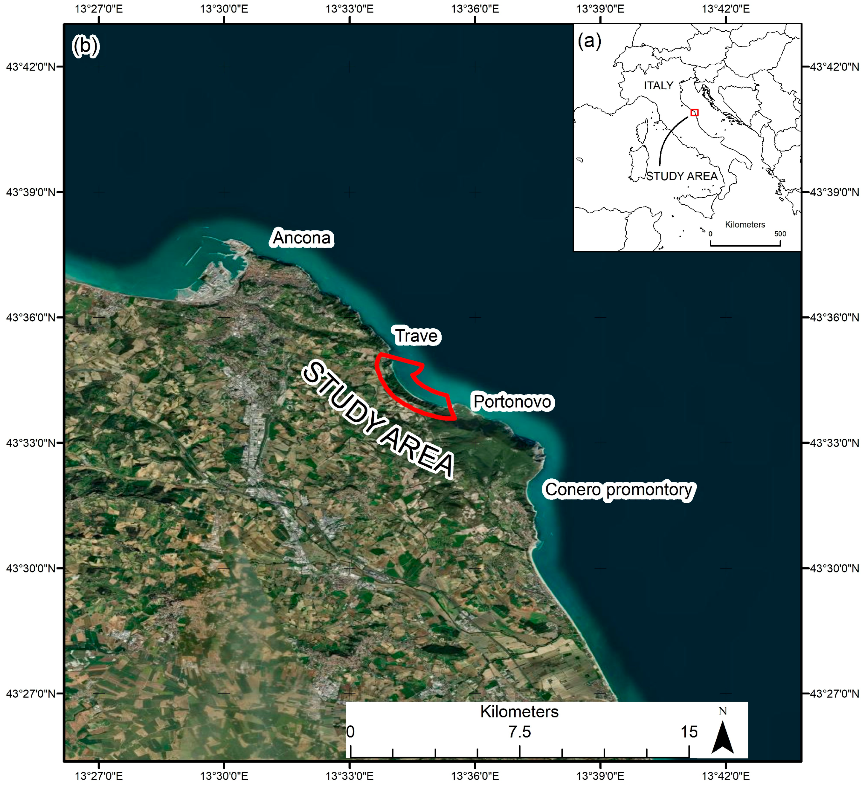
Figure 1. (a) Location map of the study area. (b) Satellite image showing the study area delimited by a red line (image taken from GeoEye satellite database, 2020).
Remotesensing 15 04120 g001
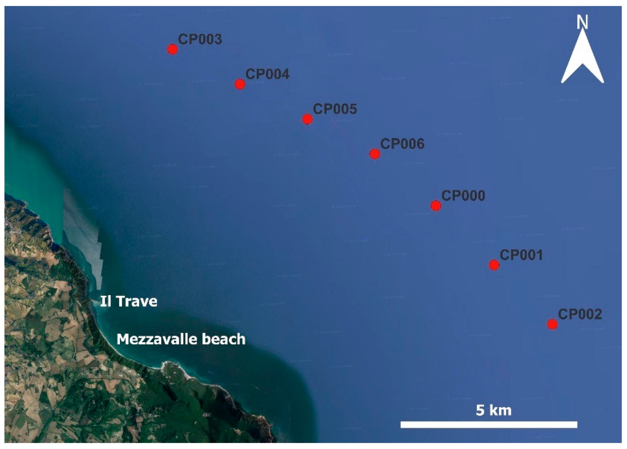
Figure 3. Coastal points defined in front of the area of interest. The points are positioned on the 20-m depth contour of the bathymetric dataset provided by ARPAE.
Remotesensing 15 04120 g003
Figure 4. Methodology followed in DSAS elaboration. (a) We used as cliff top the edge between vegetated slope and the bare cliff (showed by the red line). (b) The baseline (the blue line), i.e., the line from which all the transects origin, was created using a buffer of the identified shoreline, with the aim of obtaining transects as perpendicular as possible with respect to the coastline. (c) Image showing the baseline (in green) and the transects (in violet) obtained by DSAS elaboration.
Remotesensing 15 04120 g004
Figure 5. Picture showing distribution of different data through time. The overlap window is between 1998 and 2021.
Remotesensing 15 04120 g005
Figure 6. At Trave sector. (a) The Sapigno Fm., composed by gypsum, is thrusted on the younger Argille Azzurre Fm. The trend of coastline in this picture is N–NW/S–SE, and the attitude of the fault plane is 205/40 in Dip Direction and Dip convention. (b) Outcrop of the Argille Azzurre Fm. composed of marls, completely fractured in blocks of few centimeters.
Remotesensing 15 04120 g006
Figure 7. (a) Values of slope and (b) elevation: Trave sector shows the highest values for both the considered parameters.
Remotesensing 15 04120 g007
Figure 8. Summary of wave and rainfall parameters: (a) POT analysis of CNR–ISMAR data between 1994–2019 for the significant wave height (Hs) for coastal point CP005, showing the identified events. The peak value is highlighted by a red dot. (b) Precipitation recorded by the stations “Ancona Torrette” and “Ancona Regione RT-1638” in the period 1990–2021.
Remotesensing 15 04120 g008
Figure 9. NSM values calculated along transects, referred to the period 1978–2021: Portonovo and Trave sector showed the highest values of retreat. (a) Computed transects for the whole study area; (b) Focus at Portonovo sector; (c) Focus at Mezzavalle sector; (d) Focus at Trave sector.
Remotesensing 15 04120 g009
Figure 10. NSM values calculated along transects, referred to the period from 1998–2007: Trave sector results the most active sector. (a) Computed transects for the study area; (b) Focus at Portonovo sector; (c) Focus at Mezzavalle sector; (d) Focus at Trave sector.
Remotesensing 15 04120 g010
Figure 11. NSM values calculated along transects, referred to the period 2010–2021: Portonovo and Trave sectors result in the sectors most affected by retreating of the cliff top edge. (a) Computed transects for the study area. (b) Focus at Portonovo sector. (c) Focus at Mezzavalle sector. (d) Focus at Trave sector.
Remotesensing 15 04120 g011
Figure 12. Results of DoDs comparison in the period from 2021–2012. Every sector is displayed in detail in scale 1:10,000. Analysis shows that the biggest height differences were recorded in Trave sector. (a) Computed DoDs for the study area; (b) Focus at Portonovo sector; (c) Focus at Mezzavalle sector; (d) Focus at Trave sector.
Remotesensing 15 04120 g012
Figure 13. The geological structure of Trave cliff (GNOa (Sapigno Fm. Upper Miocene) and FAA (Argille Azzurre Fm., Lower Pliocene–Lower Pleistocene)). The main thrusts are highlighted with red lines; the red arrows indicate the sense of movement between hanging wall and footwall in orange secondary thrusts with a lower slip. The trend of coastline in this picture is N/S, and the average attitude of the fault planes identified is 200/45 in Dip Direction and Dip convention.
Remotesensing 15 04120 g013
Table 1. Spatial resolution of the orthophotos used for the cliff top retreat analysis.
Date (yr)19781998200720102021
Cell size (m)1.28 × 1.281 × 10.5 × 0.50.5 × 0.50.1 × 0.1
Table 2. Range of GSI and UCS values for the three sectors.
GSI (Flysch)UCS (MPa)
PORTONOVO50–6030–35
MEZZAVALLE/0.5–5
TRAVE15–305–30
Table 3. DSAS results for each period analyzed. Mean EPR and ECI are reported.
PeriodsPortonovoMezzavalleTrave
EPR (m/yr)ECI (m)EPR (m/yr)ECI (m)EPR (m/yr)ECI (m)
1978–2021−0.200.160.090.16−0.250.16
1998–2007−0.210.79−0.270.79−0.720.79
2010–2021−0.400.62−0.090.62−0.420.62
Disclaimer/Publisher’s Note: The statements, opinions and data contained in all publications are solely those of the individual author(s) and contributor(s) and not of MDPI and/or the editor(s). MDPI and/or the editor(s) disclaim responsibility for any injury to people or property resulting from any ideas, methods, instructions or products referred to in the content.