Abstract
Microwave radar has advantages in detection accuracy and robustness, and it is an area of active research in unmanned ground vehicles. However, the existing conventional automotive corner radar, which employs real-aperture antenna arrays, has limitations in terms of observable angle and azimuthal resolution. This paper proposes a novel 3D ArcSAR method to address this issue, which combines rotational synthetic aperture radar (SAR) and direction estimation algorithms. The method aims to reconstruct 3D images of 360° scenes and offers distinctive advantages in both azimuthal and altitudinal sensing. Nevertheless, due to the unique structural characteristics of vehicle SAR, it is limited to receiving only a single snapshot signal for 3D sensing. We propose a resolution algorithm based on ArcSAR and the iterative adaptive approach (IAA) to resolve the limitation. Furthermore, the errors in altitude angle estimation of the proposed algorithm and conventional algorithms are analyzed under various conditions, including different target spacing and signal-to-noise ratio (SNR). Finally, we design and implement a prototype of the 3D ArcSAR sensing system, which utilizes a millimeter-wave MIMO radar system and a rotating scanning mechanical system. The experimental results obtained from this prototype effectively validate the effectiveness of the proposed method.
1. Introduction
Unmanned ground vehicles, as a new type of transportation, represent the future trend in vehicle development. In recent years, many countries worldwide have recognized the significance of unmanned ground vehicles and implemented them as a national strategy supported by relevant policies. Related technologies have found initial applications in various fields, such as intelligent transportation, logistics, mines, and ports [1].
Among the key technologies in unmanned ground vehicles, real-time environmental sensing and understanding are prerequisites for platforms to accomplish their tasks autonomously [2,3]. Various environmental sensing technologies are advancing rapidly, each with its own advantages and disadvantages. Optical sensing technology excels at structured road and target recognition but falls short in detection accuracy. Multi-line LiDAR is too expensive for widespread implementation in ordinary vehicles. Infrared and ultrasonic sensing technologies have a short detection range [4,5,6]. In addition, the performance of these technologies degrades in challenging weather conditions such as darkness, rain, snow, and smoke, as well as in unstructured environments like vegetation cover [7].
As a novel means of environmental sensing for unmanned ground vehicles, microwave radar has inherent advantages in detection accuracy, cost, and environmental adaptability [8,9,10]. Consequently, it has garnered considerable attention in this research domain. Conventional automotive radar solutions, such as Continental’s corner radar ARS408, employ real-aperture antenna arrays, which exhibit limitations in terms of observable angle and azimuthal resolution [11]. ARS408 radar has azimuthal resolutions of 12.3° and 3.2° within observable angles of ±60° and ±30°, respectively [12]. Moreover, the azimuthal resolution decreases as the target deviates from the array’s normal direction.
While the forward-looking direction is important for vehicle environmental sensing, the sense of rear and side information is equally vital for urban driving and detecting surrounding obstacles. Particularly in field environments, the mobility of unmanned ground vehicles relies on obtaining complete 360° environmental information. Unfortunately, the observable angle of conventional automotive corner radar is insufficient to meet the requirements of panoramic information. Consequently, existing solutions employ at least four or more corner radars to obtain panoramic information around the vehicle, thereby increasing sensor costs.
In response to the above situation, rotational SAR uses the rotating arm to detect outside the arc. By constructing an arc-shaped synthetic aperture, the effective observable angle can cover a 360° range. As a result, this novel SAR structure has been the subject of extensive research in recent years. In the field of ground deformation monitoring, this new all-time rotational SAR system is named ArcSAR [13,14]. Among them, the 2D ArcSAR has been verified using experiments [15,16]. In rotorcraft helicopters, ROSAR generates an arc-shaped synthetic aperture to observe the ground by rotating the helicopter rotors [17,18]. Here, we refer to the above SAR systems collectively as ArcSAR. While ArcSAR exhibits advantages in terms of azimuthal resolution and consistency, the current research efforts have mainly focused on 2D imaging, and the realization of 3D panoramic sensing based on microwave radar remains unaccomplished within the field of vehicle applications [19]. The absence of height information can result in distortions in the projected targets within 2D imaging results, leading to errors in target identification and distance estimation.
To address the problem of absent height information, this paper proposes a novel 3D ArcSAR method, which combines rotational SAR and direction estimation algorithms to reconstruct 3D images of 360° scenes. The 3D ArcSAR sensing system employs a millimeter-wave radar with multiple receivers installed at the end of the rotating arm to estimate the altitude angle, enabling 3D panoramic imaging during rotation. This ability enhances the accuracy of environmental understanding in road scenarios. Moreover, this system achieves panoramic 3D imaging with just one rotational scan by one radar.
As the 3D ArcSAR platform rotates during the scanning process, the location of the rotating arm is in constant change. Altitude angle estimation poses a challenge as only a single snapshot signal can be received per angle. Common resolution algorithms such as Music and APES require multiple snapshot signals to construct the sample covariance matrix, and the matrix would lose rank when only a snapshot signal is received [20,21,22]. Attempting to attain a full-rank sample covariance matrix by reducing the dimension of the matrix results in estimates with reduced resolution and robustness. The FFT algorithm does not require multiple snapshot signals, but its angle resolution is poor with a limited number of array antennas. Orthogonal Matching Pursuit (OMP) is a signal reconstruction algorithm that requires the number of targets to be known in advance [23,24]. IAA is a spectral estimation algorithm based on weighted least squares (WLS) estimation proposed by Li Jian at the University of Florida in 2010 [25,26,27], which has demonstrated good results in linear aperture experiments. In order to overcome the single snapshot limitation, we designed an IAA resolution algorithm based on circular apertures, which exhibits improved adaptability for unmanned ground vehicles.
In this paper, we propose the 3D ArcSAR method as a solution to the deficiencies in the sensing performance of conventional automotive radar in both azimuthal and altitudinal directions. To overcome the limitation that the vehicle SAR can only receive a single snapshot signal in 3D sensing, we designed a dedicated IAA resolution algorithm for this specific case. The main contributions of this paper are summarized as follows.
- The 3D ArcSAR method is proposed for reconstructing panoramic 3D images with rotational SAR and direction estimation techniques. This method effectively addresses the limitations of existing automotive corner radar systems, including shortcomings in altitude direction sensing, azimuthal resolution, and consistency. The 3D ArcSAR sensing system achieves panoramic 3D imaging with only one radar and one rotation scan. Therefore, it reduces the number and complexity of devices required and can better meet the sensing needs of unmanned ground vehicles.
- A resolution algorithm based on IAA was designed specifically for 3D ArcSAR. This algorithm overcomes the limitation of receiving only a single snapshot signal per angle. We analyze the errors in altitude angle estimation for both the proposed algorithm and conventional algorithms under varying conditions, such as target spacing and SNR. The proposed algorithm has superior resolution in the case of single snap, small antenna arrays, and an unknown number of targets compared to other existing methods.
- The 3D ArcSAR prototype is designed based on a millimeter-wave radar system and a rotating mechanical system. The radar system employs a low-cost, readily available commercial off-the-shelf (COTS) radar, facilitating easy deployment. The rotating mechanical system is designed to adapt to different scenes, with adjustable rotation speed and arm length. Additionally, it can be remotely controlled by a computer to facilitate experiments. The 3D ArcSAR prototype validates the superior resolution accuracy performance of the proposed algorithm and can be further utilized for experiments in various scenes in the future.
The remaining sections of this paper are organized as follows. Section 2 provides a detailed description of the model structure and the fundamental principles underlying rotational SAR imaging and direction estimation in 3D ArcSAR. In Section 3, simulations of 3D ArcSAR are conducted and the errors in altitude angle estimation for both the proposed algorithm and conventional algorithms under varying conditions are analysed. Section 4 presents the designed prototype of the 3D ArcSAR sensing system and provides the experimental results obtained with this prototype. Finally, conclusions are drawn in Section 5.
2. Three-Dimensional ArcSAR and Signal Processing
2.1. Signal Model and Geometry Model
2.1.1. 2D Structure of ArcSAR
Figure 1 shows a schematic diagram of ArcSAR’s 2D structure. It consists of a rotating arm extending from the central location of the rotating platform and a SAR radar system P for transmit and receive signals. The x and y axes indicate two mutually perpendicular directions parallel to the ground.
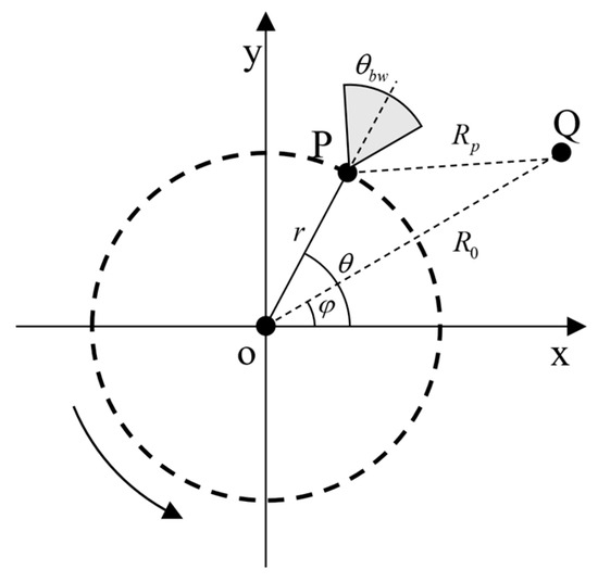
Figure 1.
Schematic diagram of ArcSAR’s 2D structure.
The rotating plane of the SAR radar system is chosen as the imaging plane. Q is the target (assume Q is on the imaging plane). is the rotating angle of the rotating arm. is the azimuth angle of the target. is the antenna beam width. is the distance between Q and the center of the platform. is the distance between Q and P, which can be expressed as
The time difference between the transmit signal and the receive signal can be expressed as
Take the linear frequency modulation continuous wave (LFMCW) as an example, and the transmit and receive signal models of LFMCW can be expressed as
where and represent the time variation in the fast time dimension and the sweep time of each chirp signal. and represent the carrier frequency and LFMCW slope. represents the scattering coefficient.
In addition, the beamwidth of the antenna is considered. After dechirp processing, the echo signal can be expressed as
2.1.2. Direction Estimation with Multiple Receivers
Figure 2 shows the geometric structure of the 3D ArcSAR sensing system, which acquires altitude information in the altitude direction by an antenna array. Combined with the antenna array and the azimuthal synthetic aperture produced by the antenna sweep, the system is able to generate panoramic 3D images. Here, the antenna array is configured as a uniform array. The z-axis indicates the direction perpendicular to the ground.
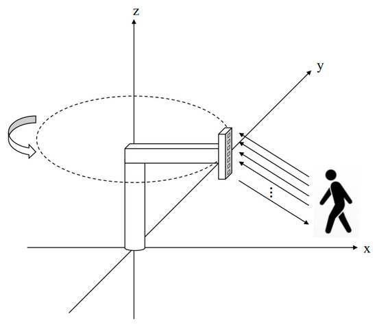
Figure 2.
Geometric structure of the 3D ArcSAR sensing system.
Figure 3 shows the distance difference in receive signals between the different antennas. According to the fundamental principle in the direction estimation with multiple receivers, the signal travels further in the second antenna than the first.
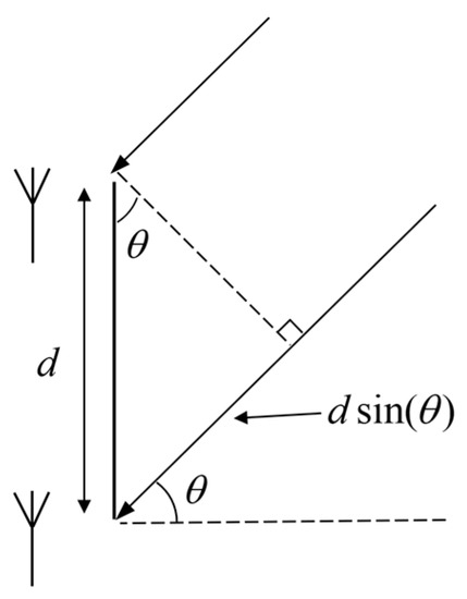
Figure 3.
Schematic diagram of the distance difference in receive signals between the different antennas.
The speed of electromagnetic waves is equal to the speed of light . Then, the above distance difference is calculated to the time difference, assuming that the array configuration consists of antennas, with the first antenna serving as the reference point. Therefore, the time difference of each antenna is
Relative to the first antenna, the phase difference of the signal arriving at each antenna is
The receive signal is defined as , where is expressed as the number of snapshots of the receive signal. Then, the signal received by the multiple antenna array is
where represents the steering vector, and it contains the angle information.
For a uniform linear array, the signal containing information about directions can be expressed as
For a given antenna array, the mathematical form of the steering vector is known. As a result, FFT can be applied for altitude angle estimation according to Equation (8).
directions are chosen equally within the angle range, and the steering matrix can be expressed as
The inner product of this steering matrix and the receive signal with the target angle can be expressed as
where the inner product result is a scalar array. It goes through all the angles to find the maximum value, and the angle corresponding to the maximum value represents the estimated target angle.
In addition, for a uniform linear array with a known antenna spacing and number of antennas, the Rayleigh limit resolution of the altitude angle estimation is
where represents the number of antennas. represents the antenna spacing, and is generally chosen.
2.2. Panoramic Image Formation by the Back Projection Algorithm
The Back Projection Algorithm (BPA) is a widely used SAR imaging algorithm. Unlike the existing ArcSAR frequency domain algorithms, which require a certain imaging angle, BPA utilizes azimuth accumulation imaging, enabling imaging at any azimuth position without restrictions on the size of the imaging angle. This feature makes BPA particularly advantageous for vehicle-mounted ArcSAR real-time perception, as it allows imaging results to be obtained at any desired azimuth position during platform rotation. Furthermore, BPA exhibits excellent parallelism, enabling real-time processing through multi-core parallel computing [28].
BPA can be described in four key steps:
- Distance compression.
Distance compression is the matched filtering process. In the dechirp system, the received echo signal from each antenna can be directly sampled and FFT-processed to obtain the distance compression results. Without considering the beamwidth of the antennas, the result of the FFT of the signal (5) can be expressed as
where represents the parameter unrelated to , and represents the time difference between the transmit and receive signal at the target Q position. Equation (13) can observe that the target Q is compressed to the frequency , which gives preliminary distance information.
- 2.
- Data interpolation resampling.
In step 1, only the signal time difference between the radar system P and the target Q is considered for a particular moment. However, in order to cover the entire sensing range, it is essential to calculate the signal time differences for the complete range.
Interpolation resampling is employed subsequent to the distance compression process. The detection range is partitioned into a grid, with distance gates set in each direction. The time difference between the transmit and receive signal at each distance gate position is represented by . Additionally, the frequency is represented by . The signal after interpolation resampling can be expressed as
It is evident that the magnitude of reaches its maximum when is taken to .
- 3.
- Compensating for delayed phase.
The delayed phase is the additional phase of the echo signal relative to the transmit signal. In order to achieve phase-coherent accumulation of the echo signal from the same target at different moments, it is necessary to compensate for the delayed phase at each moment. The delayed phase compensation factor can be expressed as
The delayed phase compensation factor (16) and the data in step 2 are multiplied to obtain the echo signal amplitude , which can be expressed as
- 4.
- Phase-coherent accumulation.
The position of the signal transmitted by the SAR system is constantly changing. In ArcSAR, the radar system P can receive the echo signal of the target Q on a segment of the circular trajectory. The angle size of this circular trajectory is equal to the beamwidth of the antenna.
Following that, a section of azimuthal data with an angle range equal to the antenna beamwidth are selected, and a window function with the same angle range is used to weight this section of data. The data values under this scene can be obtained as
where represents the weighted window function.
The above four steps are systematically repeated for every position within the entire 360° scene. Finally, the resulting output is a 2D panoramic image.
It is known that the radial resolution is related to the signal bandwidth, and the azimuth resolution is related to the synthetic aperture length. However, in ArcSAR, the synthetic aperture length is determined by combining the arm length and the antenna beamwidth. As a result, the theoretical resolution in the radial and azimuth directions can be expressed as
where and represents the bandwidth and central wavelength of the signal. The weighted window process widens the main lobe. Moreover, represents the compensation for the weighted window function. For example, the compensation of the Hanning window is about 1.6269.
2.3. IAA-Based Angle Estimation in Altitude Direction
Due to the structure of the 3D ArcSAR sensing system, the antenna array obtains only one snapshot signal for each azimuth direction. As a result, common algorithms such as APES and Music are unsuitable for this scenario. These algorithms require multiple snapshots of the signal when constructing the sample covariance matrix since a full-rank matrix cannot be achieved from a single snapshot signal alone. Attempting to attain a full-rank sample covariance matrix by reducing the dimension of the matrix results in estimates with reduced resolution and robustness. The FFT algorithm, which employs the inner product of the echo signal and the steering vector for angle estimation, can be applied with a single snapshot. However, it is affected by sidelobe interference, resulting in a reduction in estimation resolution.
In contrast, IAA is an iterative algorithm that utilizes the relationship between the sample covariance matrix and the complex scattering coefficients. It initializes the iterations with the FFT results and constructs the signal covariance matrix with the results of the previous iteration. This algorithm can reduce the effect of sidelobes while maintaining the same number of receivers, resulting in enhanced resolution and improved 3D imaging capabilities.
Similar to the FFT, the signal model can be mathematically expressed as
where represents the echo signal received by antennas on the 3D ArcSAR at a particular moment, commonly called the measurement signal. is the steering matrix and is the estimated signal. is additive white Gaussian noise (AWGN).
The idea of the least square estimation is to find a linear unbiased estimate , such that is minimized. Also, by introducing the weighting matrix , the optimization problem of WLS can be expressed as
The solution of the above equation is as follows:
where represents the conjugate transpose. IAA is equivalent to the WLS problem when is the interference-plus-noise covariance matrix of the signal .
is a diagonal matrix of , and the elements on the diagonal of are the scattering coefficients in the directions.
where represents the mathematical expectation.
Assuming that and are known, the signal covariance matrix can be expressed as
In practice, only is known about the echo signal, while is unknown. can be expressed as
Assuming that the scattering coefficient of each direction in is expressed by , the interference-plus-noise covariance matrix is defined as
The scattering coefficient is replaced by the unbiased estimate of it, which is obtained by substituting Equation (23) into (24)
According to the principle of matrix inversion, Equation (28) can also be written as
From the above equations, can be calculated from . should be initialized as the unit matrix first. Since is unknown, the initialized can be expressed as
When is a unit matrix, the result of IAA is equivalent to FFT. IAA takes the result of FFT as the initial value of and then iteratively updates and based on their interrelationships until the convergence condition is reached. In general, the estimation performance does not improve significantly after more than eight iterations. At this time, it is reasonable to consider the algorithm to have reached convergence.
In practice, when the condition number of is large, the calculation of matrix inversion may be inaccurate or even non-invertible. To solve this problem, a diagonal loading approach can be taken to regularize . Thus, can be expressed as
where is the diagonal matrix. The elements on the diagonal represent the estimates of the noise, and these can be expressed as
where is column of the unit matrix.
The specific steps of the IAA based on 3D ArcSAR include the following:
- Determine the spatial coordinates of the targets and extract the signals from multiple receivers corresponding to these specific locations.
- Employ IAA to estimate the altitude angle at the designated target locations.
- Generate sets of SAR images of the 2D scenes through the application of BPA to process the received signal from each antenna. Obtain a complete 3D panoramic image combined with the height dimension information obtained by IAA.
First, initialize the scattering coefficient estimate and the noise estimation matrix .
Perform iterations according to the interrelationship of Equations (35)–(39) until convergence.
Finally, the obtained scattering coefficient of the echoes can be expressed as
where the altitude angle estimation of the corresponding location is combined with the 2D SAR panoramic imaging results to obtain a 3D image of the scene.
3. Parametric Analysis in Simulations
The 3D ArcSAR method proposed in this paper was evaluated using simulation experiments. This section presents an analysis of the performance of ArcSAR 2D imaging and 3D imaging. Additionally, the errors in altitude angle estimation between the proposed algorithm and the common algorithms are analyzed, considering different target spacing and SNR.
3.1. Imaging Simulation
3.1.1. Imaging of 2D ArcSAR
In order to verify the performance of 2D ArcSAR imaging, we set up the simulation experiments. The main parameters are shown in Table 1.

Table 1.
Experimental parameters of 2D ArcSAR imaging.
According to Equations (19) and (20), the theoretical resolution can be obtained under these experimental parameters. In particular, Hanning windows are added to the distance processing, and cos windows are added to the azimuthal processing. The radial resolution is 0.158m, and the azimuthal resolution is 0.34°.
In this experiment, we set six point targets surrounding the system. These targets were placed at 12 m, 15 m, and 18 m, with azimuth angles of 90° and 150°. The imaging results of the target array are shown in Figure 4. The horizontal axis of the coordinate system indicates the azimuthal direction, and the vertical axis indicates the radial direction.
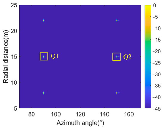
Figure 4.
Simulation of imaging results for the point targets.
Subsequently, we selected Q1 and Q2 for analysis, marked in Figure 4. The imaging results of these two targets were sliced, and the corresponding impulse response results are presented in Figure 5 and Figure 6. Their quality parameters are shown in Table 2.
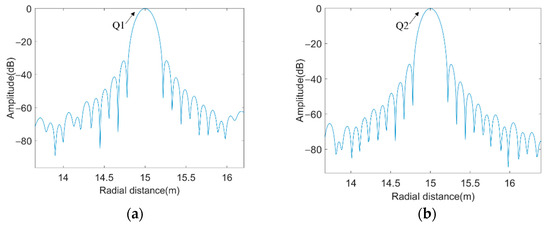
Figure 5.
Radial impulse responses: (a) Q1; (b) Q2.
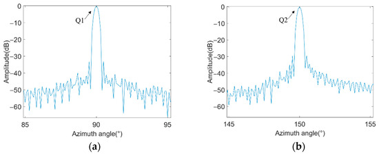
Figure 6.
Azimuthal impulse responses: (a) Q1; (b) Q2.
Table 2.
Simulation results quality parameters.
The inclusion of different window functions in the radial and azimuthal directions resulted in different main lobe spreading and sidelobe attenuation. Specifically, Hanning windows were applied for distance processing, while cos windows were applied for azimuthal processing. According to Table 2, we observed that the radial and azimuthal resolutions were in general agreement with the theoretical values. The results of Peak Sidelobe Ratio (PSLR) and Integrated Sidelobe Ratio (ISLR) were within the reasonable range.
3.1.2. Imaging of 3D ArcSAR
The proposed 3D ArcSAR method was analyzed via a simulation, with an SNR of 10 dB and an AD frequency of 45.5 MHz. The rest of the main parameters are shown in Table 1. The number of antenna array elements was set to 16, and the antenna array had a length of 14.4mm and a spacing of 0.96mm. Referring to Equation (12), the Rayleigh limit resolution of this antenna array was 6.35°.
The parameters of the set coordinate system are expressed as the distance between the target and the turntable center, the azimuthal angle, and the altitudinal angle, respectively. In this experiment, we placed seven targets in the 3D scene, which were located at (10 m, 90°, 0°), (15 m, 80°, 0°), (15 m, 100°, 0°), (15 m, 90°, 0°), (15 m, 90°, 6°), (20 m, 90°, 0°) and (20 m, 90°, 12°), and these target location relationships in the 3D scene are shown in Figure 7. Among them, the turntable center of the 3D ArcSAR sensing system was located at (0 m, 90°, 0°).
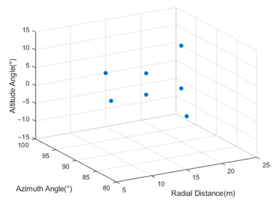
Figure 7.
Target location relationships in 3D scenes.
Following the rotational scan, the received signals from each antenna undergo 2D ArcSAR imaging processing. Figure 8 displays the eighth antenna’s 2D imaging results. It is important to highlight that the 2D imaging results exhibited a stacked masking phenomenon at (15 m, 90°) and (20 m, 90°), where two targets with differing heights were located.
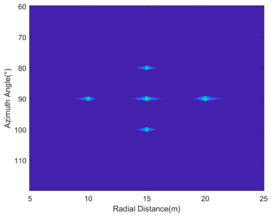
Figure 8.
Two-dimensional imaging results of the eighth antenna.
The above results were directly employed for 3D image processing, as shown in Figure 9.
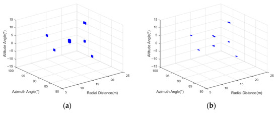
Figure 9.
Imaging results of 3D ArcSAR: (a) FFT; (b) IAA.
The target spacing at (15 m, 90°) and (20 m, 90°) were 6° and 12°. The phase information of the echo signals at these two locations was extracted, and the angle estimation was performed by FFT, OMP, and IAA, respectively. The achieved angle estimation results are depicted in Figure 10. Due to the target spacing at (15 m, 90°) exceeding the Riley limit resolution, FFT could not distinguish the two targets. Conversely, both OMP and IAA exhibited resolutions that surpassed the Rayleigh limit resolution. Figure 10a shows that the angle estimation results of OMP were inaccurate. Consequently, the next subsection thoroughly analyzes the errors in altitude angle estimation of different algorithms, considering the influence of different target spacing and SNR.
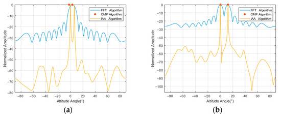
Figure 10.
The altitude angle estimation results: (a) target spacing is 6°; (b) target spacing is 12°.
3.2. Performance Analysis of Different Algorithms Influenced by Different Factors
3.2.1. Target Spacing
Music can attain the full-rank sample covariance matrix by reducing the dimensionality of the matrix, enabling angle estimation under a single snap signal. Therefore, we added a contrastive analysis of Music in this section, where we processed a single snap signal of 16 antenna array elements into a 9-snap signal of 8 elements.
We analyzed the accuracy of angle estimation under different target spacing. Target 2 was set at a fixed altitude angle of 0°, while the altitude angle of Target 1 was variable. The angle spacing between them was linearly varied from 15° to 3.8° with steps of 0.05°. Assuming that the SNR was 35dB and there were 16 antenna array elements, the altitude direction of the targets was estimated by different resolution algorithms. The errors in altitude angle estimation were then determined through a comparison between the estimated and true values. The relative error analysis for Target 1 is shown in Figure 11.
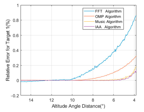
Figure 11.
The relative error in the angle estimation for Target 1 under different target spacing.
The results indicate that the IAA algorithm outperformed the FFT, OMP, and Music algorithms in terms of angle resolution. The error in altitude angle estimation increased gradually from approximately 12° and 9° for FFT and OMP, respectively, while the values were about 5.5° for Music and IAA. However, Music exhibited a slightly higher angle estimation error compared to IAA for narrow spacing conditions.
3.2.2. SNR
We analyzed the angle estimation performance under different SNRs. In this simulation, the number of antenna elements was still fixed at 16. To ensure the optimal resolution for all algorithms at different SNRs, the target spacing was set to 12°. We analyzed where the SNR ranged from −15 dB to 35 dB in steps of 0.25 dB, repeated 10,000 times. The analysis of the relative error for Target 1 is shown in Figure 12.
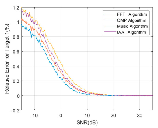
Figure 12.
The relative error in the angle estimation for Target 1 under different SNRs.
The findings demonstrate that as the SNR decreased, the angle resolution also decreased. All these algorithms exhibited robustness to changes in the SNR. Specifically, FFT exhibited superior resolution performance under low-SNR conditions, while IAA excelled under high SNR conditions. Music with a reduced matrix dimension had no performance advantage.
However, similar to OMP, Music requires the target signal to be sparse in spatial location and necessitates prior knowledge of the number of targets. These requirements can present challenges for accurate angle estimation in practical, real-world scenarios. As a result, Music and OMP may not be suitable for applications when an unknown number of scattering targets are stacked in similar locations.
4. Imaging Analysis in Experiments
4.1. The Experimental System
There is little domestic and international research on the 3D SAR imaging of rotational structures. In order to validate the feasibility of the 3D ArcSAR sensing system and its associated imaging processing techniques, it was necessary to construct a 3D ArcSAR imaging platform.
We designed the 3D ArcSAR sensing system prototype to facilitate the acquisition of 3D panoramic imaging data. The prototype consisted of a millimeter-wave MIMO radar system and a rotating scanning mechanical system, as shown in Figure 13. The radar was mounted at the end of the rotating arm, while the MIMO antenna was set up in the altitude direction. By rotating the arm, the system can generate an azimuthal synthetic aperture and uses the MIMO antenna for altitude angle estimation. With the capability to be mounted on the roof of an unmanned ground vehicle, this system enables the acquisition of high-quality 3D imaging results in a 360° range surrounding the vehicle.
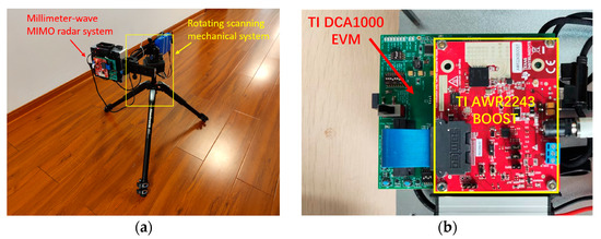
Figure 13.
(a) The 3D ArcSAR sensing system. (b) The millimeter-wave MIMO radar system.
The millimeter-wave MIMO radar system consists of the TI AWR2243BOOST radar and the TI DCA1000EVM real-time data capture adapter. TI AWR2243BOOST is equipped with three transmit antennas and four receive antennas, where the separation between adjacent receive antennas is set as . However, these transmit antennas are not arranged in parallel. Therefore, only the first and third transmit antennas can be used to achieve the desired MIMO radar. The angle resolution of the millimeter-wave MIMO radar is about 12.69°. The rotating scanning mechanical system consists of a rotary base, a rotating arm, and a rotating motor. The rotating motor is electrically assisted and can be remotely controlled for speed and steering by a computer. The modular design of the mechanical system allows the flexible adjustment of the arm length to accommodate diverse experimental requirements.
4.2. Two-Dimensional Experimental Results of ArcSAR
In this experiment, metal corner reflectors are used to simulate point targets. The main parameters of the ArcSAR system based on millimeter-wave MIMO radar are shown in Table 3.
Table 3.
Experimental parameters.
We placed two metal corner reflectors, Q1 and Q2, spaced 90° apart. Both Q1 and Q2 were situated at a radial distance of about 8.4 m from the rotation center. Figure 14 shows the relationship diagram between the targets and the ArcSAR system’s location.
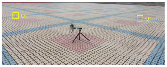
Figure 14.
The relationship diagram between the targets and the ArcSAR system’s location.
To show the ArcSAR 2D imaging results visually, we converted the polar coordinate system of the imaging results into the rectangular coordinate system. The imaging results of the two metal corner reflectors Q1 and Q2 in the polar coordinate system and rectangular coordinate system are shown in Figure 15a,b.
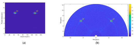
Figure 15.
Two-dimensional imaging results of the targets: (a) polar coordinate system; (b) rectangular coordinate system.
Subsequently, the imaging results for Q1 and Q2 were analyzed. The imaging results were sliced, and the corresponding impulse response results in the azimuthal direction are shown in Figure 16. Their quality parameters are shown in Table 4.
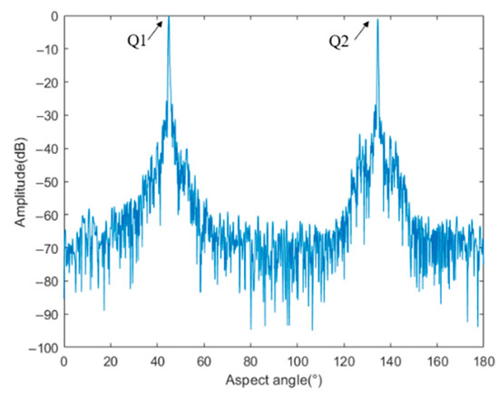
Figure 16.
Azimuthal impulse responses of Q1 and Q2.
Table 4.
Quality parameters of experimental results.
Based on the above results, it can be observed that the measured azimuthal resolution deviated by approximately 10% from the theoretical value. This discrepancy can be attributed to the comparatively lower SNR encountered in the real measurement environment. The results of PSLR and ISLR were within the reasonable range.
4.3. Three-Dimensional ArcSAR Experiments
In this experimental phase, the primary focus was on verifying the altitudinal resolution performance of the 3D ArcSAR system. The FM slope and turntable arm length were adjusted to 50 MHz/us and 0.395 m, respectively. The rest of the main parameters were the same as in Table 3, with the antenna array comprising eight elements.
Two reflectors were positioned at different altitudinal locations, and the altitudinal distance between them was 0.64 m. The millimeter-wave radar system’s plane was situated at a height of 0.43 m, while the horizontal distance between the rotating scanning mechanical system’s center and the targets measured 1.53 m. The true values of the targets’ altitudinal angles were determined to be about −7.81° and 15.69°, respectively. Figure 17 displays the spatial relationship between the targets and the 3D ArcSAR system.
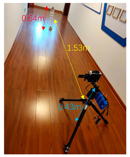
Figure 17.
The spatial relationship between the targets and the 3D ArcSAR system.
Considering the proximity of these two targets in the 2D imaging, it was necessary to perform angle estimation in the altitudinal direction. The 2D and 3D imaging results acquired through the utilization of the proposed algorithm for stacked masking targets are shown in Figure 18. Observing Figure 18a suggests that the two targets do not seem to be entirely stacked. However, it is known after processing that these two targets still have stacked parts of each other.
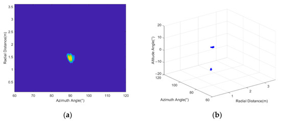
Figure 18.
Imaging results under stacked masking targets: (a) 2D; (b) 3D.
The echo data from the stacked location of the two targets were analyzed, and the altitude angle estimation results after processing are shown in Figure 19. Both OMP and IAA could distinguish the two targets well, and IAA was able to determine that the angles of the two targets in the altitudinal direction were about −6.6° and 13.3°. This angle spacing was larger than the Rayleigh limit resolution of the AWR2243BOOST radar with two-transmitter and four-receiver antennas. Consequently, FFT could also distinguish the two targets. However, the angle estimation results of FFT were not too satisfactory due to factors such as a low SNR and sidelobe interference within the real measurement.
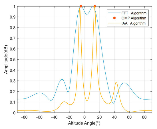
Figure 19.
The altitude angle estimation results under stacked masking targets.
Furthermore, we conducted experiments involving a near-circular step structure, as shown in Figure 20, to evaluate the performance of the 3D ArcSAR imaging method in real-world scenarios. Due to the particular structure of the steps, each step can occupy a different location in the 2D plane and altitudinal direction. Therefore, this scene was well suited to verifying the real effect of the 3D ArcSAR imaging method, and this step structure comprised five levels. The 3D ArcSAR system was located at an approximate distance of 8 m from the steps, with the radar antenna elevated to a height of about 0.55 m over the ground.
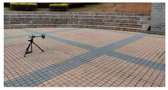
Figure 20.
The relationship diagram between the steps and the 3D ArcSAR system’s location.
In order to expand the detection distance and enhance the azimuth resolution of the 3D ArcSAR system, the pulse width was adjusted to 68.3 us, and the turntable arm length was increased to 0.5085 m here.
The proposed algorithm was used to image the targets, and the 2D and 3D imaging results are shown in Figure 21.
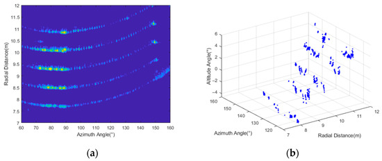
Figure 21.
Imaging results of the steps: (a) 2D; (b) 3D.
Figure 21 demonstrates that the various levels of steps exhibited distinguishable differences in radial distance and altitudinal direction. The proposed method successfully facilitated the imaging and distinction of the steps. It should be noted that Figure 21b portrays altitude angles below 0° in the imaging results, which was due to the radar antenna’s location above some of the steps. These experimental results can verify the rationality and accuracy of the designed 3D ArcSAR system.
5. Conclusions
The proposed 3D ArcSAR method enables the reconstruction of 3D panoramic images through panoramic rotational SAR and direction estimation. To address the limitations encountered in vehicle 3D sensing, particularly the reliance on a single snapshot signal, we designed an IAA-based resolution algorithm specifically for the 3D ArcSAR sensing system. At the same time, the errors in altitude angle estimation for both the proposed algorithm and the conventional algorithms were analyzed, considering various factors such as target spacing and SNR. It was demonstrated that the proposed algorithm has superior resolution in the case of single snap, small antenna arrays, and an unknown number of targets compared to other existing methods.
Additionally, we designed a prototype of 3D ArcSAR based on a 77GHz COTS radar and a rotating scanning mechanical system. This prototype serves the purpose of validating the proposed algorithms presented in this paper, and can be further utilized for experiments in various scenes in the future.
While our primary focus was on addressing the specific challenges of unmanned ground vehicle applications, we recognize that the proposed 3D ArcSAR sensing system holds significant potential for remote sensing applications. We propose the following potential “remote sensing” applications:
- Environmental Monitoring: The 3D ArcSAR system’s panoramic imaging capability can be leveraged for monitoring large-scale environmental areas, such as forests, coastal regions, and agricultural landscapes. It can provide valuable insights into vegetation growth, land use changes, and environmental dynamics.
- Disaster Management: During natural disasters such as floods, earthquakes, and landslides, the 3D ArcSAR system can efficiently gather information on the affected areas and aid in disaster response and management efforts. The system’s ability to acquire 3D images in real-time can be crucial for assessing the extent of damage and planning relief operations.
- Climate Change Studies: The system’s capacity to monitor vast areas with high accuracy enables data collection for climate change studies. It can be used to monitor ice caps, glaciers, and polar regions, providing critical data for understanding climate change patterns.
However, the current work is still at a preliminary stage. In the next stage, we plan to conduct further in-depth research on various aspects, including the experimental verification of complex targets, more efficient ArcSAR imaging algorithms, and the impact on the ArcSAR imaging results under the motion of unmanned ground vehicles.
Author Contributions
Conceptualization, Y.H., J.W. and X.H.; methodology, Y.H. and J.W.; software, J.W.; validation, Y.H., J.W. and D.F.; formal analysis, Y.H.; investigation, Y.H.; resources, J.W., X.H. and D.F.; data curation, Y.H. and J.W.; writing—original draft preparation, Y.H.; writing—review and editing, J.W. and X.H.; visualization, Y.H.; supervision, J.W.; project administration, J.W. and X.H.; funding acquisition, J.W. and D.F. All authors have read and agreed to the published version of the manuscript.
Funding
This research was funded by the National Natural Science Foundation of China, grant number 62101562.
Data Availability Statement
The experiment data are available on request.
Conflicts of Interest
The authors declare no conflict of interest.
References
- Wang, S.; Jiang, X. Three-Dimensional Cooperative Positioning in Vehicular Ad-hoc Networks. IEEE Trans. Intell. Transp. Syst. 2021, 22, 937–950. [Google Scholar] [CrossRef]
- Sun, S.; Petropulu, A.P.; Poor, H.V. MIMO Radar for Advanced Driver-Assistance Systems and Autonomous Driving: Advantages and Challenges. IEEE Signal Process. Mag. 2020, 37, 98–117. [Google Scholar] [CrossRef]
- Engels, F.; Heidenreich, P.; Wintermantel, M.; Stacker, L.; Al Kadi, M.; Zoubir, A.M. Automotive Radar Signal Processing: Research Directions and Practical Challenges. IEEE J. Sel. Top. Signal Process. 2021, 15, 865–878. [Google Scholar] [CrossRef]
- Bilik, I. Comparative Analysis of Radar and Lidar Technologies for Automotive Applications. IEEE Intell. Transp. Syst. Mag. 2023, 15, 244–269. [Google Scholar] [CrossRef]
- Li, Y.; Ibanez-Guzman, J. Lidar for Autonomous Driving: The Principles, Challenges, and Trends for Automotive Lidar and Perception Systems. IEEE Signal Process. Mag. 2020, 37, 50–61. [Google Scholar]
- Subedi, D.; Jha, A.; Tyapin, I.; Hovland, G. Camera-LiDAR Data Fusion for Autonomous Mooring Operation. In Proceedings of the 2020 15th IEEE Conference on Industrial Electronics and Applications (ICIEA), Kristiansand, Norway, 9 November 2020; pp. 1176–1181. [Google Scholar]
- Gong, J.; Duan, Y.; Liu, K.; Chen, Y.; Xiong, G.; Chen, H. A robust multistrategy unmanned ground vehicle navigation method using laser radar. In Proceedings of the 2009 IEEE Intelligent Vehicles Symposium, Xi’an, China, 3 June 2009; pp. 417–424. [Google Scholar]
- Li, Y.; Shang, X. Multipath Ghost Target Identification for Automotive MIMO Radar. In Proceedings of the 2022 IEEE 96th Vehicular Technology Conference (VTC2022-Fall), London, UK, 26 September 2022; pp. 1–5. [Google Scholar]
- Gusland, D.; Torvik, B.; Finden, E.; Gulbrandsen, F.; Smestad, R. Imaging radar for navigation and surveillance on an autonomous unmanned ground vehicle capable of detecting obstacles obscured by vegetation. In Proceedings of the 2019 IEEE Radar Conference (RadarConf), Boston, MA, USA, 22 April 2019; pp. 1–6. [Google Scholar]
- Zhu, J.; Song, Y.; Jiang, N.; Xie, Z.; Fan, C.; Huang, X. Enhanced Doppler Resolution and Sidelobe Suppression Performance for Golay Complementary Waveform. Remote Sens. 2023, 15, 2452. [Google Scholar] [CrossRef]
- Infineon and Oculii Partner to Accelerate Imaging Radar Software Technology Solutions in Automotive Applications. Available online: https://www.businesswire.com/news/home/20191218005069/en/Infineon-Oculii-Partner-Accelerate-Imaging-Radar-Software (accessed on 18 December 2019).
- Domhof, J.; Happee, R.; Jonker, P. Multi-sensor object tracking performance limits by the Cramer-Rao lower bound. In Proceedings of the 2017 20th International Conference on Information Fusion (Fusion), Xi’an, China, 10 July 2017; pp. 1–8. [Google Scholar]
- Gao, Z.; Jia, Y.; Liu, S.; Zhang, X. A 2-D Frequency-Domain Imaging Algorithm for Ground-Based SFCW-ArcSAR. IEEE Trans. Geosci. Remote Sens. 2022, 60, 1–14. [Google Scholar] [CrossRef]
- Zhang, Y.; Wang, Y.; Schmitt, M.; Yuan, C. Efficient ArcSAR Focusing in the Wavenumber Domain. IEEE Trans. Geosci. Remote Sens. 2022, 60, 1–10. [Google Scholar] [CrossRef]
- Pieraccini, M.; Miccinesi, L. ArcSAR: Theory, Simulations, and Experimental Verification. IEEE Trans. Microw. Theory Tech. 2017, 65, 293–301. [Google Scholar] [CrossRef]
- Lin, Y.; Liu, Y.; Wang, Y.; Ye, S.; Zhang, Y.; Li, Y.; Li, W.; Qu, H.; Hong, W. Frequency Domain Panoramic Imaging Algorithm for Ground-Based ArcSAR. Sensors 2020, 20, 7027. [Google Scholar] [CrossRef]
- Li, W.; Liao, G.; Zhu, S.; Zeng, C.; Xu, J. A Novel Clutter Suppression Method Based on Time-Doppler Chirp Varying for Helicopter- Borne Single-Channel RoSAR System. IEEE Geosci. Remote Sens. Lett. 2022, 19, 1–5. [Google Scholar] [CrossRef]
- Li, W.; Liao, G.; Zhu, S.; Xu, J. A Novel Helicopter-Borne RoSAR Imaging Algorithm Based on the Azimuth Chirp z transform. IEEE Geosci. Remote Sens. Lett. 2019, 16, 226–230. [Google Scholar] [CrossRef]
- Nan, Y.; Huang, X.; Guo, Y.J. A Panoramic Synthetic Aperture Radar. IEEE Trans. Geosci. Remote Sens. 2022, 60, 1–13. [Google Scholar] [CrossRef]
- Li, J.; Stoica, P. An adaptive filtering approach to spectral estimation and SAR imaging. IEEE Trans. Signal Processing. 1996, 44, 1469–1484. [Google Scholar] [CrossRef]
- Schmidt, R.O. Multiple emitter location and signal parameter estimation. IEEE Trans. Antennas Propagation. 1986, 34, 276–280. [Google Scholar] [CrossRef]
- Shang, X.; Liu, J.; Li, J. Multiple Object Localization and Vital Sign Monitoring Using IR-UWB MIMO Radar. IEEE Trans. Aerosp. Electron. Systems. 2020, 56, 4437–4450. [Google Scholar] [CrossRef]
- Simoni, R.; Mateos-Nunez, D.; Gonzalez-Huici, M.A.; Correas-Serrano, A. Height estimation for automotive MIMO radar with group-sparse reconstruction. Electr. Eng. Syst. Sci. 2019. [Google Scholar] [CrossRef]
- Jafri, M.; Srivastava, S.; Anwer, S.; Jagannatham, A.K. Sparse Parameter Estimation and Imaging in mmWave MIMO Radar Systems With Multiple Stationary and Mobile Targets. IEEE Access 2022, 10, 132836–132852. [Google Scholar] [CrossRef]
- Roberts, W.; Stoica, P.; Li, J.; Yardibi, T.; Sadjadi, F. Iterative Adaptive Approaches to MIMO Radar Imaging. IEEE J. Sel. Top. Signal Process 2010, 4, 5–20. [Google Scholar] [CrossRef]
- Yardibi, T.; Li, J.; Stoica, P.; Xue, M.; Baggeroer, A.B. Source Localization and Sensing: A Nonparametric Iterative Adaptive Approach Based on Weighted Least Squares. IEEE Trans. Aerosp. Electron. Syst. 2010, 46, 425–443. [Google Scholar] [CrossRef]
- Guo, Y.; Zhang, D.; Li, Q.; Zhang, P.; Liang, Y. FIAA-Based Super-Resolution Forward-Looking Radar Imaging Method for Maneuvering Platforms. In Proceedings of the 2022 3rd China International SAR Symposium (CISS), Shanghai, China, 2 November 2022; pp. 1–5. [Google Scholar]
- Suren, C.; Evelina, A.; Anreas, K.; Alessandro, M. Reviewing GPU architectures to build efficient back projection for parallel geometries. J. Real-Time Image Process. 2020, 17, 1331–1373. [Google Scholar]
Disclaimer/Publisher’s Note: The statements, opinions and data contained in all publications are solely those of the individual author(s) and contributor(s) and not of MDPI and/or the editor(s). MDPI and/or the editor(s) disclaim responsibility for any injury to people or property resulting from any ideas, methods, instructions or products referred to in the content. |
© 2023 by the authors. Licensee MDPI, Basel, Switzerland. This article is an open access article distributed under the terms and conditions of the Creative Commons Attribution (CC BY) license (https://creativecommons.org/licenses/by/4.0/).