Article

Introducing ICEDAP: An ‘Iterative Coastal Embayment Delineation and Analysis Process’ with Applications for the Management of Coastal Change

by
Nicholas B. Wellbrock
1,2,
Nathalie W. Jung
1,
David P. Retchless
1,*,
Timothy M. Dellapenna
1,2 and
Victoria L. Salgado
1
1
Department of Marine and Coastal Environmental Science, Texas A&M University at Galveston, Galveston, TX 77554, USA
2
Department of Oceanography, Texas A&M University, College Station, TX 77843, USA
*
Author to whom correspondence should be addressed.
Remote Sens. 2023, 15(16), 4034; https://doi.org/10.3390/rs15164034
Submission received: 30 June 2023 / Revised: 4 August 2023 / Accepted: 12 August 2023 / Published: 15 August 2023
(This article belongs to the Special Issue Advances in Remote Sensing of the Inland and Coastal Water Zones II)

Abstract

:
Coastal embayments provide vital benefits to both nature and humans alike in the form of ecosystem services, access to waterways, and general aesthetic appeal. These coastal interfaces are therefore often subject to human development and modifications, with estuarine embayments especially likely to have been anthropogenically altered. Frequent alterations include damming to eliminate tidal influx, backfilling to create new land, and development for the sake of economic gain, which may cause profound damage to local habitats. By providing a record of transitions in surface waters over time, satellite imagery is essential to monitoring these coastal changes, especially on regional to global scales. However, prior work has not provided a straightforward way to use these satellite-derived datasets to specifically delineate embayed waters, limiting researchers’ ability to focus their analyses on this ecologically and economically important subset of coastal waters. Here, we created ICEDAP, a geometry-based ArcGIS toolbox to automatically delineate coastal embayments and quantify coastal surface water change. We then applied ICEDAP to the coast of South Korea, and found that coastal habitat change was particularly profound within embayed regions identified using an 8 km epsilon convexity setting (denoting a moderate distance from the coast and degree of enclosure by surrounding land areas). In the mapped coastal embayments, more than 1400 km2 of coastal habitats were lost during the past 38 years, primarily due to human modification such as large-scale land reclamation projects and the construction of impoundments. Our results suggest that anthropogenic alterations have resulted in the widespread loss of more than USD 70 million of valuable coastal ecosystem services. Together, ICEDAP provides a new innovative tool for both coastal scientists and managers to automatically identify hotspots of coastal change over large spatial and temporal scales in an epoch where anthropogenic and climate-driven changes commonly threaten the stability of coastal habitats.

Graphical Abstract

1. Introduction

Coastal systems are a vital part of the survival and growth of nature and humans alike, creating a morphological and ecological interface between land and sea [1]. Coastal systems provide important natural resources and ecosystem services such as food from finfish and shellfish, storm protection, tourism, and water filtration [2]. This wide array of opportunities provided by the coasts has therefore attracted many humans, so that more than half of the world’s population now lives in coastal areas [1,3]. There are real concerns about the conditions of coastal systems as human impacts such as major oil spills, medical waste disposal, wetland losses and impacts that lead to shellfish bed closures disrupt the natural processes of coastal ecosystems and threaten the ecological and economic values of coastal areas [3]. Excessive engineering projects have also severely degraded coastal ecosystems during the last century, making them increasingly vulnerable to external influences and, concurrently, more susceptible to regime shifts [4,5]. For example, field observations have shown that estuarine dam constructions have significantly altered local sediment fluxes and tidal energy as well as river discharge, and resulted in major shifts towards more wave-dominated systems [6,7,8]. Numerous seawalls associated with land reclamation projects, river divergence projects, or agricultural use of irrigation and drainage canals [9,10] have previously been shown to decrease associated estuaries’ water storage capacity and cause severe flooding nearby [11,12]. Diking and filling of coastal habitats removes important habitat for fish and waterfowl, introduces invasive species, and disturbs local plant and animal communities, with the potential for further alterations of the estuary’s water quality and biotic communities [13].
Embayments are coastal inlets semi-protected from open-ocean processes; if such inlets contain a freshwater input, then they are also considered to be estuaries, and may be referred to as estuarine embayments [14]. Despite their ecological, economic, and social importance, coastal features like embayments and estuaries have remained understudied. Only in the last few decades, with the advancement in remote sensing techniques and availability of satellite imagery, have researchers begun to gain a more synoptic perspective on the complexity and variety of these dynamic coastal ecosystems [1]. One of the primary obstacles to studies of changes in embayed and estuarine waters—especially on regional to global scales—has been the lack of consistent and generalizable methods for delineating these waters. As early as the mid-20th century, researchers had produced global maps showing the locations—but not shapes or extents—of embayed coasts [15]. Drawing on advances in remote sensing and digital mapping, more recent work has provided significantly more detailed and precise depictions of coastal waters, but has remained inconsistent in its mapping of embayed and estuarine areas, especially when defining their seaward extents. In Europe, the EU Water Framework Directive has required EU member states to map their “coastal” waters, including all waters within 1 nautical mile (nm, 1.85 km) of each state’s baseline and any “transitional” (i.e., estuarine) waters beyond that baseline. However, as noted by [16], member states have been inconsistent in their application of the relevant EU directives, due in large part to ambiguity about the standards and datasets that should be used to define transitional waters. In the US, the Coastal Zone Management Act of 1972 expansively defines coastal waters as any waters within US jurisdiction that are adjacent to the coastline and contain “a measurable quantity or percentage of seawater.” The authors in [17] provide a helpful table summarizing the varied definitions of the coastal zone employed by a selection of national and subnational jurisdictions; considering only the seaward side of this definition, standards for defining extents vary widely, including those based on natural processes (e.g., mean tidal level at lower low water), distance from a shoreline or baseline (from 0 to 12 nm), depth (e.g., 30 m isobath), and geopolitical boundaries (e.g., outer limits of the territorial sea). On the academic side, researchers have considered many standards and methods for delineating coastal and/or estuarine waters. However, despite attempts to aid coastal management through the identification of more ecologically coherent or easily managed units for embayed waters (such as “coastalsheds” in [17] or “semi-enclosed coastal systems” in [18]), these researchers have stopped short of providing workable solutions for mapping these waters at regional to global scales, with the techniques presented for delimiting seaward extents being especially limited. Specifically, previous research has, variously: not attempted to develop tools for consistently mapping these regions [18]; mapped only a small number of such regions over a limited geographic extent [19,20]; suggested standards that require datasets for delineating estuarine or coastal waters that are unavailable globally [16]; or given more attention to landward extents while defining seaward extents based on somewhat arbitrary standards (e.g., a line across the narrowest portion of the mouth of the estuary in [20], or the seaward edge of a country’s exclusive economic zone (EEZ) in [17]).
To meet the need for a consistent, adaptable, and easily deployable method for identifying the seaward extent of embayed coastal waters on regional to national scales, we developed and tested an ArcGIS toolbox to automatically identify and delineate embayed coastal waters. Our technique is based on an “epsilon convexity” approach, which accounts for both embayed waters’ proximity to the coast and their degree of “enclosure” by surrounding land areas. To test the effectiveness of this tool and its suitability for coastal management, we have also added tool components to measure and compare coastal change in the delineated areas. In the following sections, we describe the development of this toolbox and its testing along the shore of the South Korean peninsula, where traditional agricultural practices and coastal construction of estuarine dams have considerably modified the shoreline within the last century [6,10].

2. Materials and Methods

2.1. Iterative Coastal Embayment Delineation and Analysis Process (ICEDAP)
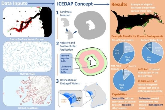
2.1.1. Overview

The inputs, workflow, and outputs of the Iterative Coastal Embayment Delineation and Analysis Process (ICEDAP) tool are shown in Figure 1. ICEDAP is one of the first set of tools that automatically identifies and delineates coastal embayments at user-defined embayment sizes (defined by the width of the mouth of the concave embayed region). ICEDAP includes three newly developed ArcGIS tools for embayment delineation and area change analyses across large datasets with no additional processing or post-editing (Figure 1). The toolbox was created and tested with ArcGIS Pro version 3.1.
With the advancement in remote sensing techniques, there is an emerging number of image-processing methodologies that attempt to automatically measure channel width and dynamics [21,22,23,24,25,26,27,28,29,30,31]. However, the majority of tools require the input of pre-processed channel masks, and were specifically developed for riverine systems. For example, previous work created a new set of efficient tools that map and measure changes in channel widths, the locations and rates of migration, accretion and erosion, and the spacetime characteristics of cutoff dynamics, but heavily depend on manual pre-editing of composite images in order to generate binary channel masks [21]. While many riverine processes and dynamics are comparable to those of coastal embayments, embayments commonly extend beyond the location of stream mouths and generally include marine (i.e., tides and waves) as well as fluvial influences. This is particularly important as coastal embayments are hotspots of environmental change [30,31]. For example, more than 7000 km2 of intertidal area within embayments have been directly converted to either urban or agricultural fields in the Yellow Sea over the last five decades [32]. Although more recent tool development efforts specifically targeted estuarine systems and their spatial and temporal change with the attempt to minimize user interference and the need for additional processing or post-editing [31], the toolbox still lacks the necessary means to create a pre-defined channel mask. We therefore created the new toolbox, ICEDAP, that not only automatically delineates coastal embayments (therefore eliminating the need for manual pre-processing of riverine channel masks), but also extends the focus of analyses towards more holistic coastal regions, facilitating analyses of hotspots of anthropogenic and climate-driven change.

2.1.2. Input

ICEDAP requires the input of four different data sets: the Global Surface Water Dataset (GSWD, including both the maximum water extent dataset and the occurrence change intensity dataset), the HydroSHEDS streamline dataset, coastal boundary line vectors, and the EEZ line dataset (Table 1). The GSWD provides the yearly extent of the seasonal (tidal flats) and permanent (open water) water occurrence between 1984 and 2021, with a pixel resolution of 30 m × 30 m [33]. Here, the maximum water extent dataset provides information on all the locations ever detected as water over the 38-year period, whereas the occurrence change intensity dataset provides information on where and how much surface water occurrence increased, decreased or remained the same from 1984–1999 and 2000–2021 [33]. We used the maximum water extent dataset to delineate the maximum spatial extent of estuarine bodies, whereas we used the occurrence change intensity to estimate areal change between 1984 and 2021 within identified estuaries. Here, we used Google Earth Engine to automatically clip the GSWD maximum water extent dataset to the user-specified country boundaries and convert the dataset to a format compatible with the ICEDAP toolbox (i.e., shapefile) (see Supplementary Material) (Table 1). We note that the maximum water extent and occurrence change intensity datasets can also be obtained directly from the Global Surface Water Explorer website (https://global-surface-water.appspot.com/download, accessed on 1 September 2022). However, website-derived data would need to be manually processed to be used by the ICEDAP toolbox, and temporal analyses of yearly coastal change would require the Google Earth Engine tool for data preparation, as the GSWD yearly occurrence dataset is only available on Google Earth Engine. The HydroSHEDS streamline dataset is a gridded hydrography dataset derived from digital elevation models (https://www.hydrosheds.org/products, accessed on 1 September 2022), showing the location of rivers worldwide with a resolution of 15 arc seconds. We used the HydroSHEDS streamline dataset in an effort to identify land masses with hydrologic characteristics that may support estuarine processes as well as potential estuarine embayments. The EEZ dataset contains a combination of both land and maritime boundaries to represent country boundaries with the EEZ (i.e., an area of the ocean, generally extending 200 nm or 370 km beyond a nation’s territorial sea, within which a coastal nation has jurisdiction over both living and nonliving resources [34]) (https://www.marineregions.org, accessed on 1 September 2022). The global coastline dataset consists of a 1:10 million small-scale physical line vectors that represent the global coastlines, including major islands (https://naturalearthdata.com, accessed on 1 September 2022). Both the EEZ and global coastline datasets were used to isolate the selected study country. All datasets have global coverage so that they can be applied to any country. For more local studies, the datasets can be exchanged for high-resolution alternatives.

2.1.3. Buffer Application

The coastal embayment delineation and analysis process consists of three individual sub-tools: (1) landmass separation and embayment delineation, (2) buffer adjustment, and (3) coastal surface water change analysis. Together, these create a semi-automated process capable of delineating the extent of embayments for a singular region and its respective landmasses, via the maximum extent of surface water and an adapted coastline generalization process. These extent features are used to create accurate masks of surface water changes within embayed coastal waters.
The coastal feature identification and delineation process applies a series of geometry-focused tools to delineate the seaward extent of coastal embayments. We build on the work of [35,36,37,38], who created and refined a cartographic generalization technique known as epsilon convexity: by tracing the path of a circle with a defined diameter as it is rolled along a line, bends in the line that are too sharp to fit the rolling circle (segments of “epsilon non-convexity”) are identified and removed, thereby simplifying the line. As described in [38] and in the Embayment Delineation Section, this “rolling circle” process can be replicated in GIS software (e.g., ArcGIS Pro version 3.1) using a series of buffers. Instead of using these methods to strictly draw the generalized line for a coastal bend as [38] did, here it is modified to use the coastal bend line as the exterior of an embayment, while still maintaining the inner geometry of the coastline and inlets.

Landmass Separation

In preparation of buffer application, land within the study area is separated into individual landmass components, or islands. This prevents unintentional artifacts between close-proximity landmasses and allows for a logical embayment organizational scheme corresponding to the respective landmass. Using GSWD maximum-extent surface waters, landmasses are created as an inverse of the surface water extents through a series of bounding polygons and erasure of surface waters (Figure 2). These are separated into their own features so they can be run through the landmass filtering process, which uses HydroSHEDs stream data to filter out landmasses lacking streams, as they typically lack the necessary size to be compatible with ICEDAP’s buffer sizes. The remaining landmasses are then sorted by area and assigned a ranking from greatest to least.

Embayment Delineation

Enlarged, inverted versions of landmasses are needed during the application of the “circle method” to remove non-embayed waters and limit the extent of processing (Figure 3). A 1 km buffer is first applied to each landmass to create a generalized extent. To this, a 250 km buffer is applied, and the original (Figure 3a), detailed landmass is erased from the center of the 250 km buffered polygon (Figure 3b). This creates an inversion of the landmass, an annulus, or “donutesque” shape, with the inner void instead being the landmass and the ring providing a barrier for processing. The inverted polygon is then simplified to a tolerance equal to the resolution of the surface water data (30 m), to reduce geometries with excess vertices which are incompatible with certain GIS tools. Additionally, voids equal to or less than 50 km2 are filled to remove artifacts of the landmass separation process and simplification tool.
ICEDAP then applies a series of user-defined buffers in an effort to delineate the seaward extent of our coastal embayments. Similar to [38], in the rolling of a circle along the coastline, our modified process simulates this by using a series of sequential negative and positive geometric buffers (ranging from 1, 2, 4, 8, 16, 32, 64, 128, and 256 km) to create nine separate products to delineate distinct, individual polygons representing embayments and sub-embayments along the coast. These values were chosen as they represent a geometric series (with the exception of 1 km, which was chosen to provide increased detail on a larger scale) of progressively increasing buffer sizes, similar to Horton’s application of geometric series to develop stream orders [39]. This geometric series approach removes a level of subjectivity when determining buffer sizes for a specific region. These buffer products are used to trim away any seaward surface water from the embayment, leaving the remaining landward waters up to approximately 10 km inland, the distance used by Sayre in a similar, regionwide analysis of the identification of coastal and island features [40]. Inflows with channel widths less than 0 m are not considered, as the resolution of the inputs to the HydroSHEDS model do not allow for the delineation of narrower stream features.
The negative buffer is first applied to the inverted landmass polygon, pulling the polygon’s edge away from the coastline equal to the specified buffer size (Figure 3c). This distance is synonymous with the radius of the “circle” which we are simulating. In specific cases, application of the negative buffer may create gaps of missing surface water that may form between larger embayed inland water bodies significantly wider than their mouths. This leaves embayment polygons “stranded” inland which are found to be nearly 0.05% or less in area than the primary polygon being buffered. ICEDAP therefore removes all polygons with a size of less than 0.05% of the primary polygon. A positive version of the same buffer size is then applied in order to push the boundary back toward the landmass, drawing a seaward embayment extent similar to that which would exist if a circle of a similar size were to be rolled along the coastline, a product representing a generalized version of the coastline (Figure 3d).
The final embayment delineation involves erasing this positive buffer product from the original inverted landmass polygon (Figure 3e). This removes non-embayed surface water data, with only embayed surface waters remaining. Prior to this, an artifact cleaner removed stray pixels by applying a 150 m buffer to the outer bound of the original bounding polygon by overlapping where the pixels would be created during the final erasing. This is merged with the final buffer product to form a singular geometry, and the final erasing is applied. The resulting product is a multi-featured polygon, with each individual feature representing an embayed waterbody serving as a mask for raster extraction for the specific buffer size applied. This appears as a “ring” of embayed waters around the particular landmass. This tool is rerun for each of the nine buffer sizes from 1 km to 256 km (Figure 3f).

Buffer Adjustment

In some cases, the areal extent of individual embayments within the same parent buffer does not necessarily increase with buffer size (e.g., the areal extent of the 128 km embayment exceeds the areal extent of the 256 km embayment). Here, we created an additional tool to identify embayments where the areal extent did not strictly increase with each buffer size or remained unchanged. ICEDAP preserves all embayments but creates an additional variable to differentiate between embayments that increase in areal extent along with buffer size (1) and those that do not (0).

Coastal Surface Water Change

To automatically measure coastal surface water change, ICEDAP extracts occurrence change intensity for each embayment, based on the GSWD [29]. Here, the tool identifies pixels of gain, loss, and no change, and calculates the areal extent of each category by multiplying the pixel count by the pixel resolution (i.e., 30 × 30 m). Because the Global Surface Water Occurrence Change Intensity dataset provides further information about the degree of change (i.e., percent change), ICEDAP includes a secondary component to quantify intensity-adjusted areal change by multiplying extent loss or gain by percent change.

2.1.4. Output

ICEDAP creates a shapefile and text file for each individual embayment as output. Each text file contains information on the location of the embayment as well as total area lost, gained, and unchanged for each buffer size contained within the same 256 km embayment. The shapefile contains geospatial information for each embayment. Together, information provided by the shapefiles and text files can be visually displayed and analyzed with other programs such as ArcGIS (ArcGIS Pro version 3.1) and MATLAB (MATLAB R2022a).

2.2. ICEDAP Application and Case Study

2.2.1. Study Site

South Korea is located in East Asia on the southern portion of the Korean Peninsula, where high mountains along the east coast and gentler topography towards the west coast contribute to the formation of the four major drainage basins within the country (i.e., Han, Geum, Yeongsan, and Nakdong) (Figure 4). While high-density population centers along the major rivers largely contribute to downstream discharge and development [41], the geography and geological characteristics of the Korean Peninsula contribute to the formation of the area’s primary estuarine classification: rias. Rias are non-glaciated, incised river valleys, which have been inundated by the sea over time as sea level rises [42,43]. These are commonly characterized by a moderate relief as well as a V-shaped valley, and typically meander inland from the sea with smaller inlets branching outwards, easily recognized from above by their dendritic features [42]. Ria estuaries in South Korea can be found along the low-to-moderate-relief western and southern coast, with only a few being found on the east coast, due to the much steeper topography (Figure 4). Reflecting these geomorphological differences, the South Korean coast is split into three regions for our analysis: the west coast (from the North Korean border to Songho-Ri), the south coast (from Songho-Ri to Busan), and the east coast (from Busan to the North Korean border).
Throughout the past century, South Korea has experienced a large amount of anthropogenically driven change within its coastal zone. This wave of change has been motivated by government policies implemented in the late 20th century to boost agricultural and industrial activity and water policy reforms occurring from the early 1900s to the present day [41,45]. Approximately half of the previously identified 463 estuaries are classified as closed, following the installment of an estuarine dam or sluice gate [46], and more than 1000 km2 of tidal flats have been reclaimed since the 1940s [47,48]. These anthropogenic alterations have not only removed valuable habitat space, but have also restricted the entry of saltwater/discharge of freshwater, disrupted the sediment budget, and impacted the long-term morphology of the system, leading to major shifts in estuary processes and ecosystem balance [6]. For example, the construction of estuarine dams and numerous seawalls in the Nakdong Estuary have significantly altered the timing of the local sediment flux and tidal energy as well as river discharge, and resulted in the formation of barrier islands and the shift from a tide-dominated system to a more wave-dominated system [6]. South Korea’s geomorpholocical variance of embayments combined with its elevated level of coastal development provides an optimal “test bed” for developing a embayment-focused, coastal-change-analysis process.

2.2.2. Breakpoint Analysis

Previous work defined the estuary mouth as the transition point from river to coastal embayment [49,50], whereas other work commonly places the estuary mouth at the bay entrance and therefore includes portions of the bay farther offshore [51]. Here, we used a breakpoint analysis to determine which buffer size most adequately represents the seaward extent of our embayments while also capturing the majority of coastal change. We compared relative surface water loss and gain (i.e., relative to the total surface water loss/gain in the 256 km buffer) to changes in buffer size for each embayment, and defined the breakpoint as the point closest to the intersection between the minimum and maximum derivative. Here, we first interpolated and smoothed relative surface water loss and gain for each embayment and buffer size and used MATLAB’s gradient function to create a collection of vectors pointing in the direction of increasing water loss or gain. We then identified the buffer size closest to the intersection between the gentlest gradient/slope (i.e., generally between buffer sizes 32–256 km) and the steepest gradient/slope (i.e., generally between buffer sizes 1–2 km). We then calculated the mean, mode, and median values for all breakpoints in order to identify a common breakpoint across all South Korean embayments (Figure 5).

2.2.3. Anthropogenic Alterations

To determine the extent of human impacts on South Korea’s estuaries, we manually identified the location of dams within all embayments. Here, we defined dams as any anthropogenic structure that prevents saltwater intrusion (i.e., estuarine dams, sluice gates, seawalls, submerged weirs, etc.). We then manually eliminated portions of the estuary that have turned into freshwater lakes or are now being used for agricultural purposes.

2.2.4. Algorithm Accuracy and Validation

The accuracy of our surface water change analyses largely depends on the accuracy of the GSWD on which this study is based [33]. Validation processes at the pixel scale suggest that the GSWD identifies the location of water occurrence with high precision and accuracy (accuracy > 95%) [33]. Additional mapping efforts along the South Korean coast suggest that the GSWD is reliable for high-resolution coastal change analyses [50]. Because the Global Surface Water Change Intensity dataset compares change in water occurrence intensity between two epochs (i.e., 16 March 1984 to 31 December 1999, and 1 January 2000 to 31 December 2021) rather than two individual time steps, quantitative accuracy and validation efforts remain difficult. In addition to relying on earlier accuracy assessments of the GSWD, we spot-checked our results by comparing them with high-resolution Google Earth images of selected embayments along the South Korean coast in 1984 and 2021.

3. Results

3.1. Distribution and Size of South Korean Embayments

We identified a total of 43, 64, 88, 147, 259, 508, 932, 1661, and 2476 embayments for the 256 km, 128 km, 64 km, 32 km, 16 km, 8 km, 4 km, 2 km, and 1 km buffers, respectively. At the same time, surface water area within identified embayments decreased with buffer size: from 30,583 km2, 24,653 km2, 12,900 km2, 7066 km2, 5286 km2, 4467 km2, 2976 km2, 2031 km2 to 1416 km2 for the same range of buffer sizes (Figure 6 and Figure 7, Table 2). Simple linear regressions suggest a significant inverse correlation between buffer size and the number of estuaries (p << 0.05; r = −0.97), as well as a significant correlation between buffer size and surface water area (p << 0.05; r = 0.97). Overall, the number and areal extent of identified embayments across the South Korean peninsula largely varied depending on the buffer size, with the larger buffer sizes resulting in fewer but larger embayments (Figure 6 and Figure 7, Table 2).
Although the majority of embayments are located along the east coast of South Korea (42%), they contain only 14% of the country’s total coastal surface water area. Approximately 37% of South Korea’s embayments are located along the west coast, containing 55% of the country’s surface water area. The remaining 22% of South Korea’s embayments are found along the south coast, occupying about 31% of surface water area. In general, the South Korean west coast is characterized by a wider and shallower continental shelf, with vast areas of intertidal sand and mudflats that have formed in a tide-dominated environment [52] and is therefore home to some of the country’s largest estuaries (Figure 6 and Figure 7). On the other hand, the South Korean east coast faces a narrow continental shelf and slope with a width of only 10–20 km and a steepness of 0.4° [53], so that estuaries tend to be smaller but more widespread (Figure 6 and Figure 7). Additionally, the tidal range along the South Korean coast varies significantly between 1 m along the east coast and 10.5 m along the northwestern part of the peninsula [54], where larger estuaries are commonly found along the tide-dominated portion of South Korea.

3.2. Surface Water Change

South Korean embayments occupied between 1477.2 ± 92.9 (1 SD) km2 (1 km buffer) and 19,894.6 ± 1235.2 km2 (256 km buffer) of surface water in 1984, and the same embayments occupied between 1192.4 ± 74.0 km2 and 18,392.2 ± 1123.5 km2 of surface water in 2021, where surface area increased with buffer size (Figure 7, Table 2). Summed across the entire country, South Korean embayments gained between 425.3 ± 32.1 and 700.3 ± 46.6 km2 of surface water between 1984 and 2021, depending on buffer size. At the same time, South Korean embayments lost between 710.1 ± 48.7 and 2203 ± 158.9 km2 of surface water, resulting in a total net area loss ranging from −284.8 ± 27.1 to −1502 ± 119.5 km2 (Figure 7, Table 2). Prominent examples of surface water loss include the coastal regions around the Han River, Incheon; Saemangeum Estuary, Gunsan; Yeongsan Estuary, Mokpo; and Nakdong Estuary, Busan (Figure 8), which are known to have undergone tremendous coastal change following port development and large-scale land reclamation projects [6,47,55,56,57,58]. Overall, approximately 86% of net surface water change within South Korean embayments occurred along the west coast (Figure 7 and Figure 8). The remaining change (12%) occurred along the south coast, with only 2% of change occurring along the west coast. We note that our estimates of coastal surface water change only include ICEDAP’s automatic area change measurements (see Coastal Surface Water Change Section) and not area change estimates from manual dam removal analyses (see Section 2.2.3. Anthropogenic Alterations).
More detailed analyses revealed an abrupt change in surface water gain and loss relative to buffer size (Figure 5). Relative water change (i.e., water change relative to the maximum observed change in the 256 km buffer) first increased sharply within the first few buffer sizes, and then progressively leveled off (Figure 5). Breakpoint analyses identified a common 8 km breakpoint for all embayments, after which surface water change remained negligible. Here, differences between individual embayments may reflect more local factors such as disturbance events, human alterations, etc. Similarly, the majority of surface water change (i.e., 90% of change) also occurred within the first 8 km from the river mouth (Figure 5).
Comparisons between pre- and post-development embayments (i.e., after manually removing portions of the coastal waters behind estuarine dams, seawalls, etc.) suggest that humans have substantially altered South Korea’s coastal systems (Figure 9). The impoundment of coastal embayments resulted in the removal of 709.1 to 16,364.0 km2 of coastal surface water through either direct water-to-land conversion for residential or farming purposes (i.e., land reclamation) (Figure 9b,c) or the conversion of coastal waters to lakes through dam construction (Figure 9d). Direct human impacts have therefore effectively reduced South Korea’s coastal waters by more than half their original size during the last 38 years alone.

4. Discussion

4.1. Defining the Ocean–Coast Boundary

Although identifying and classifying coastal embayments is a crucial tool for systematic coastal management, previous work commonly disagrees on where to draw the boundary between the open ocean and coastal environment. Our finding that the 8 km buffer adequately represents embayments in South Korea contrasts with previous work that identified between 39 and 60 estuaries along the South Korean coast [49,50]. In this previous work, visual interpretation [50] or automatic processing of coastal elevation and drainage basin datasets [49] identified the estuary mouth as the transition point from river to coastal embayment. This approach most closely aligns with the ocean–coast boundary defined by our 1 and 2 km buffers, and therefore tends to overlook major coastal change, which commonly occurs further offshore, within the bay portion of the coast (Figure 5, Figure 6 and Figure 7). By focusing on sub-estuaries rather than further offshore regions, previous coastal change assessments likely underestimated the major contribution human alterations make to coastal change. For example, ref [50] reported a net loss of 102 km2 since 1985 within South Korean sub-estuaries, while our observations suggest a net loss of 285 km2 during the same time in only our smallest buffer size.
Other work commonly places the estuary mouth at the bay entrance through manual identification and therefore includes portions of the bay that are farther offshore [46,51,59]. The number of estuaries identified by regional expert opinion assessments based on their geomorphological features, natural habitat distributions, and land use characteristics (n = 463 [46]) is similar to the number of embayments identified by the 8 km buffer (n = 508) (Figure 7). Mapping efforts in the Yellow Sea found that recent land reclamation projects have decreased the tidal flat area by 32.2% between the 1980s and late 2000s [32], and analyses of direct human alterations in South Korean embayments within the 8 km buffer indicate a loss of coastal surface waters of 31.7% between 1984 and 2021 (this study) (Figure 9). Public water and agriculturally purposed reclamation records estimated the total reclaimed area since the 1950s to be over 1400 km2 [47], which is similar to our regional-scale estimates of South Korean anthropogenically driven surface water change in the 8 km buffer (1417 km2 (Figure 9)). Several observations therefore suggest that the 8 km buffer is suitable for delineating coastal embayments along the South Korean coast. However, we note that although the 8 km buffer appears to be the most adequate buffer size to represent coastal embayments in South Korea, a different buffer size may be required for countries with a different geometry, geology or degree of coastal development.

4.2. Environmental Response to Human Alterations

Human alterations to coastal habitats have long been recognized as a driving mechanism of coastal change [32,50,60]. South Korea, in particular, has scaled up the size of land reclamation projects and extended construction periods since the 1950s in an effort to create new arable land, leaving lasting impacts on the coastal communities and the marine environment [47]. Simple comparisons between pre- and post-impoundments suggest that the construction of estuarine dams and seawalls associated with land reclamation efforts has led to massive and widespread loss of valuable coastal systems of more than 1000 km2 over the past three decades. Previous work showed that seawall construction potentially leads to reduction in tidal current speed [61,62], deterioration of water quality due to sediment accumulation [63], changes in sediment flux mechanics [64,65,66], and ultimately tidal flat desertification [61,67]. In the case of the Nakdong River Estuary (Figure 4b), this has led to the reorganization of the entire estuary, causing a shift from a relatively tide-dominated system towards an increasingly wave-dominated system with barrier islands [6].
The loss of valuable coastal habitats also affects important ecosystem services, in particular the number of viable (non-collapsed) fisheries, the provision of nursery habitats such as oyster reefs, seagrass beds, and wetlands, and filtering and detoxification services provided by suspension feeders, submerged vegetation, and wetlands [68]. For example, the completion of the world’s longest seawall in the Saemangeum Estuary (Figure 4c and Figure 9d) has dramatically decreased the number of local marine species, and therefore the total marine product output not only in the North Jeolla province but also in the close-by cities of Gunsan, Gimje, and Buan, from 221,829 tons in 1991 to 103,342 tons in 2011 (53%) [69]. Although quantitative studies on the ecosystem services of South Korean tidal flats are based on American data, previous work estimated the recreational value of South Korean tidal flats to be about 507 USD per ha [70,71]. A simple interpretation of our results therefore suggests that direct human modifications have led to massive and widespread loss of approximately USD 36–83 million of valuable coastal habitats. These observations of rapid degradation of coastal habitats emphasize the vulnerability and connectivity of coastal ecosystems, where urban development and farming activities have become a “costly” practice.

4.3. Other Applications

While the focus of this work is on changes in embayed surface water over several decades, we note that this tool may be applied to any dataset with a consistent extent along the ocean–coastal interface. Furthermore, ICEDAP may be scaled down or up as the user pleases, providing a tool for local, regional, and possibly global scale analysis of embayments with the proper modification and fine tuning. Recent increased interest in coastal changes provides unique opportunities to apply ICEDAP, or processes utilizing ICEDAP’s methods, across different disciplines on these varying scales to create inventory products, management regions, or other applications which may require isolating embayments.
ICEDAP may be especially useful in delineating analysis regions for the rapidly proliferating datasets needed to manage coastal change. Sea level rise (SLR) has become an increasingly important topic for coastal scientists and managers, as we struggle to adapt to our quickly changing environment. Global SLR datasets such as the World Sea-Level Rise Dataset [72] or A New Global Coastal Database for Impact and Vulnerability Analysis to Sea-Level Rise [73,74] are useful for observing global trends in SLR or calculating vulnerabilities. Recent datasets providing comprehensive or more localized coastal change assessments are widely available for ecosystem, geological, and social applications. This includes coastline migration datasets providing temporal accounts of both past and future rates of erosion/accretion [75]. Global inventories of coastal habitats have been widely developed; these identify specific habitat types and track their changes, both for habitats overall and for specific habitats like salt marshes or mudflats [76,77,78]. Further, datasets for human development within embayed systems (e.g., land use datasets and inventories of infrastructure or other human activities) are common on local and regional scales in select geographies (but often lack global coverage). These components provide a great deal of information to coastal practitioners, have been studied widely, and are frequently supplemented by new datasets. However, the abundance of these data and their varying form factors make managing them difficult for complex coastal systems. ICEDAP may not only provide a way to delineate coastal systems into manageable components, but also a way to compile and truncate many large coastal datasets into logical management regions. Considering the abundance of data and the urgency of topics like SLR and coastal change, this ability may provide a valuable tool for quickly and easily dividing and analyzing change along large swaths of the coast.

4.4. Tool Limitations and Future Work

ICEDAP’s primary limitation is the inability to adapt its buffer size to changing geomorphology over larger study areas without a manual adjustment of the processes’ extent and individual processing on each differing area. Continued work should explore the use of ICEDAP’s large buffer size capabilities to create regional divides based on the coastal geomorphology and geometry. Further limitations include the current implementation of the 10 km coastal zone buffer on both the landward and seaward side. It is possible that some amount of water that should not be considered coastal (i.e., deeper, open-ocean waters) is being included in the final product in larger buffer sizes. Future work should consider implementation of a depth contour border on the seaward side to define coast and open ocean. On the other hand, previous work commonly defines the landward boundary based on channel convergence or the maximum extent of the saline intrusion [31,78]. Although tidal effects on the areal extent of South Korea’s coastal surface waters are likely negligible, due to the resolution of the GSWD and the massive anthropogenically driven coastal change (Figure 9; see Supplementary Material), future studies focusing on regions with higher tidal ranges and natural processes with areal changes several orders of magnitude smaller than the changes observed in this study may need to more closely attend to the timeframe of data collection and tidal range to ensure minimal tidal effects on data quality.

5. Conclusions

This study introduces ICEDAP, the first toolbox to automatically identify and delineate coastal embayments and analyze habitat change. We applied ICEDAP to the coast of South Korea with a series of varying buffer sizes, and found that coastal change was particularly profound within the 8 km buffer. In particular, coastal change was mostly driven by anthropogenic alterations such as the construction of estuarine dams and seawalls for agricultural purposes, leading to the destruction of 709.1 to 16,364.0 km2 of coastal habitats or USD 36 to 83 million of valuable ecosystem services between 1984 and 2021. Together, ICEDAP provides a new innovative tool for both coastal scientists and managers to automatically identify hotspots of coastal change over large spatial and temporal scales in an epoch where anthropogenic and climate-driven changes commonly threaten the stability of coastal habitats.

Supplementary Materials

The following are available online: https://www.mdpi.com/article/10.3390/rs15164034/s1, Text S1: Tidal Effects Analysis; Text S2: Readme for ICEDAP; Script S3: GEE JavaScript Code; Tool S4: ArcPy and ArcToolbox files for ICEDAP tool.

Author Contributions

Conceptualization, N.B.W., N.W.J., D.P.R. and V.L.S.; methodology, N.B.W., N.W.J., D.P.R. and V.L.S.; validation, N.B.W. and N.W.J.; formal analysis, N.W.J. and N.B.W.; data curation, N.B.W., N.W.J. and D.P.R.; writing—original draft preparation, N.B.W. and N.W.J.; writing—review and editing, N.B.W., N.W.J., D.P.R., T.M.D. and V.L.S.; visualization, N.B.W. and N.W.J.; supervision, D.P.R. and T.M.D.; project administration, D.P.R. and T.M.D. All authors have read and agreed to the published version of the manuscript.

Funding

This research received no external funding.

Data Availability Statement

The ICEDAP toolbox is available in the Supplementary Material.

Acknowledgments

The authors would like to acknowledge Jiabi Du for his support with the Python algorithm. The authors would like to further acknowledge the undergraduate and graduate students of the Texas A&M at Galveston Coastal Geology Lab for their role in the initial testing and ground truthing of the process’s prototype.

Conflicts of Interest

The authors declare no conflict of interest. The funders had no role in the design of the study; in the collection, analyses, or interpretation of data; in the writing of the manuscript; or in the decision to publish the results.

References

  1. Martinez, M.L.; Intralawan, A.; Vazquez, G.; Perez-Maqueo, O.; Sutton, P.; Landgrave, R. The coasts of our world: Ecological, economic and social importance. Ecol. Econ. 2007, 63, 254–272. [Google Scholar] [CrossRef]
  2. Barbier, E.B.; Hacker, S.D.; Kennedy, C.; Koch, E.W.; Stier, A.C.; Silliman, B.R. The value of estuarine and coastal ecosystem services. Ecol. Monogr. 2011, 81, 169–193. [Google Scholar] [CrossRef]
  3. Culliton, T.J.; Warren, M.A.; Goodspeed, T.R.; Remer, D.G.; Blackwell, C.M.; MacDonough, J.J. 50 years of Population Change along the Nation’s Coasts, 1960–2010; National Oceanic and Atmospheric Administration: Rockville, MD, USA, 1990; Volume 41. [Google Scholar]
  4. Gunderson, L.H.; Holling, C.S. Panarchy: Understanding Transformations in Human and Natural Systems; Island press: Washington, DC, USA, 2002. [Google Scholar]
  5. Thrush, S.F.; Halliday, J.; Hewitt, J.E.; Lohrer, A.M. The effects of habitat loss, fragmentation, and community homogenization on resilience in estuaries. Ecol. Appl. 2008, 18, 12–21. [Google Scholar] [CrossRef]
  6. Williams, J.; Dellapenna, T.; Lee, G. Shifts in depositional environments as a natural response to anthropogenic alterations: Nakdong Estuary, South Korea. Mar. Geol. 2013, 343, 47–61. [Google Scholar] [CrossRef]
  7. Barusseau, P.J.; Bă, M.; Descamps, C.; Salif Diop, E.; Diouf, B.; Kane, A.; Saos, J.L.; Soumaré, A. Morphological and sedimentological changes in the Senegal River estuary after the construction of the Diama dam. J. Afr. Earth Sci. 1998, 26, 317–326. [Google Scholar] [CrossRef]
  8. Tönis, I.E.; Stam, J.M.T.; van de Graaf, J. Morphological changes of the Haringvliet estuary after closure in 1970. Coast. Eng. 2002, 44, 191–203. [Google Scholar] [CrossRef]
  9. Crawford, G.W.; Lee, G.-A. Agricultural origins in the Korean Peninsula. Antiquity 2003, 77, 87. [Google Scholar] [CrossRef]
  10. Yoon, H.S.; Yoo, C.I.; Na, W.B.; Lee, I.C.; Ryu, C.R. Geomorphology evolution and mobility of sand barriers in the Nakdong estuary, South Korea. J. Coast. Res. 2007, 50, 358–363. [Google Scholar]
  11. Healy, M.G.; Hickey, K.R. Historic land reclamation in the intertidal wetlands of the Shannon estuary, western Ireland. J. Coast. Res. 2002, 36, 365–373. [Google Scholar] [CrossRef]
  12. Wang, W.; Liu, H.; Li, Y.; Su, J. Development and management of land reclamation in China. Ocean Coast Manag. 2014, 102, 415–425. [Google Scholar] [CrossRef]
  13. Nichols, F.H.; Cloern, J.e.; Luoma, S.N.; Peterson, D.H. The modification of an estuary. Science 1986, 231, 567–573. [Google Scholar] [CrossRef]
  14. Pritchard, D.W. What Is an Estuary: Physical Viewpoint; American Association for the Advancement of Science: Washington, DC, USA, 1967. [Google Scholar]
  15. McGill, J.T. Map of coastal landforms of the world. Geogr. Rev. 1958, 48, 402–405. [Google Scholar] [CrossRef]
  16. Liquete, C.; Somma, F.; Maes, J. A clear delimitation of coastal waters facing the EU environmental legislation: From the Water Framework Directive to the Marine Strategy Framework Directive. Environ. Sci. Policy 2011, 14, 432–444. [Google Scholar] [CrossRef]
  17. Boudreau, P.R.; Butler, M.J.A.; LeBlanc, C. Coastalshed: A term to facilitate improved management in a large diverse area of the earth’s surface. Ocean Coast. Manag. 2013, 78, 64–69. [Google Scholar] [CrossRef]
  18. Newton, A.; Icely, J.; Cristina, S.; Brito, A.; Cardoso, A.C.; Colijn, F.; Riva, S.D.; Gertz, F.; Hansen, J.W.; Holmer, M.; et al. An overview of ecological status vulnerability and future perspectives of European large shallow, semi-enclosed coastal systems, lagoons and transitional waters. Estuar. Coast. Shelf Sci. 2014, 140, 95–122. [Google Scholar]
  19. Sreeja, K.G.; Madhusoodhanan, C.G.; Eldho, T.I. Coastal zones in integrated river basin management in the West Coast of India: Delineation, boundary issues and implications. Ocean Coast. Manag. 2016, 119, 1–13. [Google Scholar]
  20. Brophy, L.S.; Greene, C.M.; Hare, V.C.; Holycross, B.; Lanier, A.; Heady, W.N.; O’Connor, K.; Imaki, H.; Haddad, T.; Dana, R. Insights into estuary habitat loss in the western United States using a new method for mapping maximum extent of tidal wetlands. PLoS ONE 2019, 14, e0218558. [Google Scholar]
  21. Aalto, R.; Lauer, J.W.; Dietrich, W.E. Spatial and temporal dynamics of sediment accumulation and exchange along Strickland River floodplains (Papua New Guinea) over decadal-to-centennial timescales. J. Geophys. Res. 2008, 113, F01S04. [Google Scholar]
  22. Pavelsky, T.M.; Smith, L.C. RivWidth: A software tool for the calculation of river widths from remotely sensed imagery. IEEE Geosci. Remote Sens. Lett. 2008, 5, 70–73. [Google Scholar] [CrossRef]
  23. O’Loughlin, F.; Trigg, M.A.; Schumann, G.J.P.; Bates, P.D. Hydraulic characterization of the middle reach of the Congo River. Water Resour. Res. 2013, 49, 5059–5070. [Google Scholar] [CrossRef]
  24. Legg, N.T.; Heimburg, C.; Collins, B.D.; Olson, P.L. The Channel Migration Toolbox: ArcGIS Tools for Measuring Stream; Department of Ecology State of Washington: Bellevue, WA, USA, 2014. [Google Scholar]
  25. Miller, Z.F.; Pavelsky, T.M.; Allen, G.H. Quantifying river form variations in the Mississippi Basin using remotely sensed imagery. Hydrol. Earth Syst. Sci. 2014, 18, 4883–4895. [Google Scholar] [CrossRef] [Green Version]
  26. Yamazaki, D.; O’Loughlin, F.; Trigg, M.A.; Miller, Z.F.; Pavelsky, T.M.; Bates, P.D. Development of the global width database for large rivers. Water Resour. Res. 2014, 50, 3467–3480. [Google Scholar] [CrossRef]
  27. Rowland, J.C.; Shelef, E.; Pope, P.A.; Muss, J.; Gangodagamage, C.; Brumby, S.P.; Wilson, C.J. A morphology independent methodology for quantifying planview river change and characteristics from remotely sensed imagery. Remote Sens. Environ. 2016, 184, 212–228. [Google Scholar] [CrossRef]
  28. Isikdogan, F.; Bovik, A.; Passalacqua, P. RivaMap: An automated river analysis and mapping engine. Remote Sens. Environ. 2017, 202, 88–97. [Google Scholar] [CrossRef]
  29. Schwenk, J.; Khandelwal, A.; Fratkin, M.; Kumar, V.; Foufoula-Georgiou, E. High spatiotemporal resolution of river planform dynamics from Landsat: The RivMAP toolbox and results from the Ucayali River. Earth Space Sci. 2016, 4, 46–75. [Google Scholar] [CrossRef]
  30. Nienhuis, J.H.; Ashton, A.D.; Edmonds, D.A.; Hoitink, A.J.F.; Kettner, A.J.; Rowland, J.C.; Törnqvist, T.E. Global-scale human impact on delta morphology has led to net land area gain. Nature 2020, 577, 514–518. [Google Scholar] [CrossRef]
  31. Jung, N.W.; Lee, G.; Jung, Y.; Figueroa, S.M.; Lagamayo, K.D.; Jo, T.-C.; Chang, J. MorphEst: An automated toolbox for measuring estuarine planform geometry from remotely sensed imagery and its application to the South Korean coast. Remote Sens. 2021, 13, 330. [Google Scholar] [CrossRef]
  32. Murray, N.J.; Clemens, R.S.; Phinn, S.R.; Possingham, H.P.; Fuller, R.A. Tracking the rapid loss of tidal wetlands in the Yellow Sea. Front. Ecol. Environ. 2014, 12, 267–272. [Google Scholar] [CrossRef] [Green Version]
  33. Pekel, J.-F.; Cottam, A.; Gorelick, N.; Belward, A.S. High-resolution mapping of global surface water and its long-term changes. Nature 2016, 540, 418–422. [Google Scholar] [CrossRef] [PubMed]
  34. NOAA Ocean Explorer. What is the “EEZ”? 2023. Available online: https://oceanexplorer.noaa.gov/facts/useez.html#:~:text=An%20%E2%80%9Cexclusive%20economic%20zone%2C%E2%80%9D,both%20living%20and%20nonliving%20resources (accessed on 1 March 2023).
  35. Perkal, J. An Attempt at Objective Generalization; Discussion Paper No. 10; Michigan Inter-University Community of Mathematical Geographers: Ann Arbor, MI, USA, 1966. [Google Scholar]
  36. Perkal, J. On the Length of Empirical Curves; Discussion Paper No. 10; Michigan Inter-University Community of Mathematical Geographers: Ann Arbor, MI, USA, 1966. [Google Scholar]
  37. Christensen, A.H. Cartographic line generalization with waterlines and medial-axes. Cartogr. Geogr. Inf. Sci. 1999, 26, 19–32. [Google Scholar] [CrossRef]
  38. Mitropoulos, V.; Xydia, A.; Nakos, B.; Bescoukis, V. The use of epsilonconvex area for attributing bends along a cartographic line. In Proceedings of the International Cartographic Conference, la Corona, Spain, 9–16 July 2005. [Google Scholar]
  39. Horton, R.E. Erosional development of streams and their drainage basins; hydrophysical approach to quantitative morphology. Bull. Geol. Soc. Am. 1945, 56, 275–370. [Google Scholar] [CrossRef] [Green Version]
  40. Sayre, R.; Noble, S.; Hamann, S.; Smith, R.; Wright, D.; Breyer, S.; Butler, K.; Van Graafeiland, K.; Frye, C.; Karagulle, D.; et al. A new 30 m resolution global shoreline vector and associated global islands database for the development of standardized ecological coastal units. J. Oper. Oceanogr. 2019, 12, S47–S56. [Google Scholar]
  41. Choi, I.C.; Shin, H.J.; Nguyen, T.; Tenhunen, J. Water policy reforms in South Korea: A historical review and ongoing challenges for sustainable water governance and management. Water 2017, 9, 717. [Google Scholar]
  42. Perillo, G.M. Definitions and geomorphologic classifications of estuaries. In Dev. Sedimentol. 1995, 53, 17–47. [Google Scholar]
  43. Evans, G.; Prego, R. Rias, estuaries and incised valleys: Is a ria an estuary? Mar. Geol. 2003, 196, 171–175. [Google Scholar] [CrossRef]
  44. Tozer, B.; Sandwell, D.T.; Smith, W.H.; Olson, C.; Beale, J.R.; Wessel, P. Global bathymetry and topography at 15 arc sec: SRTM15+. Earth Space Sci. 2019, 6, 1847–1864. [Google Scholar] [CrossRef]
  45. Koh, C.H.; Ryu, J.S.; Khim, J.S. The Saemangeum: History and controversy. J. Korean Soc. Mar. Environ. Energy 2010, 13, 327–334. [Google Scholar]
  46. Lee, K.-H.; Rho, B.-H.; Cho, H.-J.; Lee, C.-H. Estuary classification based on the characteristics of geomorphological features, natural habitat distributions and land uses. Sea 2011, 16, 53–69. [Google Scholar] [CrossRef] [Green Version]
  47. Choi, Y.R. Modernization, development and underdevelopment: Reclamation of Korean tidal flats, 1950s–2000s. Ocean Coast. Manag. 2014, 102, 426–436. [Google Scholar]
  48. Koh, C.H.; Khim, J.S. The Korean tidal flat of the Yellow Sea: Physical setting, ecosystem and management. Ocean Coast. Manag. 2014, 102, 398–414. [Google Scholar]
  49. Du, J.; Park, K.; Dellapenna, T.M.; Clay, J.M. Dramatic hydrodynamic and sedimentary responses in Galveston Bay and adjacent inner shelf to Hurricane Harvey. Sci. Total Environ. 2019, 653, 554–564. [Google Scholar] [CrossRef]
  50. Wells, J.T.; Adams, C.E., Jr.; Park, Y.-A.; Frankenberg, E.W. Morphology, sedimentology and tidal channel processes on a high-tide-range mudflat, west coast of South Korea. Mar. Geol. 1990, 95, 111–130. [Google Scholar] [CrossRef]
  51. Shin, H.C.; Kohl, C.-H. Distribution and abundance of ophiuroids on the continental shelf and slope of the East Sea (southwestern Sea of Japan), Korea. Mar. Biol. 1993, 115, 393–399. [Google Scholar] [CrossRef]
  52. National Atlas of Korea, Ocean Currents. Available online: http://nationalatlas.ngii.go.kr/pages/page_1274.php (accessed on 5 December 2020).
  53. Lee, G.; Shin, H.-J.; Kim, Y.T.; Dellapenna, T.M.; Kim, K.J.; Williams, J.; Kim, S.-Y.; Figueroa, S.M. Field investigation of siltation at a tidal harbor: North Port of Incheon, Korea. Ocean Dyn. 2019, 69, 1101–1120. [Google Scholar]
  54. Williams, J.; Dellapenna, T.; Lee, G.; Louchouarn, P. Sedimentary impacts of anthropogenic alterations on the Yeongsan Estuary, South Korea. Mar. Geol. 2014, 357, 256–271. [Google Scholar]
  55. Zhusupbekov, A.A.; Shin, E.C.; Kim, J.I.; Das, B.M.; Zarenkov, V.A. Soil improvement methods of Incheon and Astana International Airports. In Proceedings of the 16th International Conference on Soil Mechanics and Geotechnical Engineering, Osaka, Japan, 12–16 September 2005. [Google Scholar] [CrossRef]
  56. Shin, E.C.; Shin, B.-W. Construction of Inchon International Airport. In Proceedings of the Proceedings: Fourth International Conference on Case Histories in Geotechnical Engineering, St. Louis, MI, USA, 9–12 March 1998; pp. 7–17. [Google Scholar]
  57. Ministry of Environment. A Study on the Preparation of Legal Systems for Systematic Management of Estuaries. 2007. Available online: https://library.me.go.kr/#/search/detail/5503755 (accessed on 1 March 2023).
  58. Kirwan, M.L.; Megonigal, J.P. Tidal wetland stability in the face of human impacts and sea-level rise. Nature 2016, 504, 53–60. [Google Scholar]
  59. Lee, S.; Lie, H.; Song, K.; Cho, C.; Lim, E. Tidal modification and its effect on sluice-gate outflow after completion of the Saemangeum dike, South Korea. J. Oceanogr. 2008, 64, 763–776. [Google Scholar] [CrossRef]
  60. Figueroa, S.M.; Lee, G.; Chang, J.; Jung, N.W. Impact of estuarine dams on the estuarine parameter space and sediment flux decomposition: Idealized numerical modeling study. J. Geophys. Res. Oceans 2022, 127, e2021JC017829. [Google Scholar]
  61. Hahm, H. Ecological crisis and women: The case of Saemangeum Reclamation Project. ECO 2004, 7, 150–170. [Google Scholar]
  62. Figueroa, S.M.; Lee, G.; Chang, J.; Schieder, N.W.; Kim, K.; Kim, S.-Y. Evaluation of along-channel sediment flux gradients in an anthropocene estuary with an estuarine dam. Mar. Geol. 2020, 429, 106318. [Google Scholar]
  63. Chang, J.; Lee, G.; Harris, C.K.; Song, Y.; Figueroa, S.M.; Schieder, N.W.; Lagamayo, K.D. Sediment transport mechanisms in altered depositional environments of the Anthropocene Nakdong Estuary: A numerical modeling study. Mar. Geol. 2020, 430, 106364. [Google Scholar] [CrossRef]
  64. Chang, J.; Lee, G.; Harris, C.K.; Figueroa, S.M.; Jung, N.W. Relative contribution of the presence of an estuarine dam and land reclamation to sediment dynamics of the Nakdong Estuary. Front. Mar. Sci. 2023, 10, 1101658. [Google Scholar] [CrossRef]
  65. Hahm, H.; Jung, M.; Lee, D. A study of interactional relations between marine ecology and fishery in the area of Saemangeum. ECO 2011, 15, 7–37. [Google Scholar]
  66. Barbier, E.B. Progress and challenges in valuing coastal and marine ecosystem services. REEP 2012, 6, 1. [Google Scholar] [CrossRef] [Green Version]
  67. Hong, E.A. Development challenges in South Korea: Reflection on the Saemangeum land reclamation project. Disjuntiva 2022, 3, 9–17. [Google Scholar] [CrossRef]
  68. Lee, H.-D. Economic value comparisons between preservation and agricultural use of coastal wetlands. Ocean Res. 1998, 20, 145–152. [Google Scholar]
  69. Kim, J.-E. Land use management and cultural value of ecosystem services in Southwestern Korean islands. JMIC 2013, 2, 49–55. [Google Scholar] [CrossRef] [Green Version]
  70. World Bank. World Sea-Level Rise Dataset. World Bank Data Catalog. 2019. Available online: https://datacatalog.worldbank.org/search/dataset/0041449/World-Sea-Level-Rise-Dataset (accessed on 1 March 2023).
  71. Vafeidis, A.T.; Nicholls, R.J.; McFadden, L.; Tol, R.S.; Hinkel, J.; Spencer, T.; Grashoff, P.S.; Boot, G.; Klein, R.J. A new global coastal database for impact and vulnerability analysis to sea-level rise. J. Coast. Res. 2008, 24, 917–924. [Google Scholar] [CrossRef]
  72. De Groeve, J.; Kusumoto, B.; Koene, E.; Kissling, W.D.; Seijmonsbergen, A.C.; Hoeksema, B.W.; Yasuhara, M.; Norder, S.J.; Cahyarini, S.Y.; van der Geer, A.; et al. Global raster dataset on historical coastline positions and shelf sea extents since the Last Glacial Maximum. Glob. Ecol. Biogeogr. 2022, 31, 2162–2171. [Google Scholar] [CrossRef] [PubMed]
  73. Mentaschi, L.; Vousdoukas, M.I.; Pekel, J.F.; Voukouvalas, E.; Feyen, L. Global long-term observations of coastal erosion and accretion. Sci. Rep. 2018, 8, 12876. [Google Scholar] [CrossRef] [Green Version]
  74. Mcowen, C.J.; Weatherdon, L.V.; Van Bochove, J.W.; Sullivan, E.; Blyth, S.; Zockler, C.; Stanwell-Smith, D.; Kingston, N.; Martin, C.S.; Spalding, M.; et al. A global map of saltmarshes. Biodivers. Data J. 2017, 5, e11764. [Google Scholar] [CrossRef] [PubMed]
  75. Murray, N.J.; Phinn, S.R.; DeWitt, M.; Ferrari, R.; Johnston, R.; Lyons, M.B.; Clinton, N.; Thau, D.; Fuller, R.A. The global distribution and trajectory of tidal flats. Nature 2018, 565, 222–225. [Google Scholar] [CrossRef] [PubMed]
  76. Buscombe, D.; Wernette, P.; Fitzpatrick, S.; Favela, J.; Goldstein, E.B.; Enwright, N.M. A 1.2 Billion Pixel Human-Labeled Dataset for Data-Driven Classification of Coastal Environments. Sci. Data 2023, 10, 46. [Google Scholar] [CrossRef] [PubMed]
  77. Savenije, H. Salinity and Tides in Alluvial Estuaries; Elsevier: Amsterdam, The Netherlands, 2005. [Google Scholar]
  78. Prandle, D. How tides and river flows determine estuarine bathymetries. Prog. Oceanogr. 2004, 61, 1–26. [Google Scholar] [CrossRef]
Figure 1. ICEDAP workflow.
Remotesensing 15 04034 g001
Figure 2. A representation of the landmass separation process. (a) Raw maximum-extent surface water data from the GSWD [33] (blue area). (b) A bounding polygon is formed around the extent of the raw surface water data (black area). (c) The raw surface water data (black area) is erased from the bounding polygon. leaving only the landmasses remaining (gray area). (d) The landmasses are separated into individual components for processing (gray area).
Remotesensing 15 04034 g002
Figure 3. A simplified representation of the buffer series application and embayment delineation. (a) A 1 km buffer and subsequent 250 km buffer (black area) is applied to the landmass polygon (gray area). (b) The landmass is erased from the center of the buffered polygon to form an inverse version of the landmass (black area). (c) A negative buffer from the geometric series (black area) is applied to the inverse landmass (gray area). (d) A positive buffer (black area) of the same value is applied to the negatively buffered polygon (gray area). (e) The positive buffer is erased from the original inverse landmass (the result of part (b)) to form a set of embayment polygons for the applied buffer size (blue area). (f) This process can be repeated for all buffer sizes defined by the user. Example embayments for the 32 (light blue), 64 (moderate blue), and 128 km (dark blue) buffers are shown.
Remotesensing 15 04034 g003
Figure 4. (a) Study map of South Korea showing elevation and bathymetry information of the peninsula. Elevation is based on SRTM15+ [44]. The red dashed line shows the three regions: the west coast (from the North Korean border to Songho-Ri), the south coast (from Songho-Ri to Busan), and the east coast (from Busan to the North Korean border). Aerial image of (b) Nakdong Estuary in 2017 (https://earthobservatory.nasa.gov/images/92703/decades-of-growth-at-port-of-busan, accessed on 1 March 2023) and (c) Saemangeum Estuary in 2018 (https://earth.esa.int/web/earth-watching/image-of-the-week/content/-/article/saemangeum-south-korea/index.html, accessed on 1 March 2023) showing large-scale urbanization and land reclamation within the embayment. (d) Geum estuary (https://earthexplorer.usgs.gov/, accessed on 1 March 2023).
Remotesensing 15 04034 g004
Figure 5. Example of relative surface water loss between 1984 and 2021 (top figure). Gray dotted line indicates the threshold for the majority of relative water loss (i.e., 90%). Breakpoint analyses identified a common breakpoint for all embayments at 8 km (red dot in top and bottom figures). Breakpoints are identified as point closest to the intersection (red triangle) between minimum and maximum gradient (dashed red lines).
Remotesensing 15 04034 g005
Figure 6. Embayments along the South Korean coast based on different buffer sizes. The red dashed line shows the three regions: the west coast (from the North Korean border to Songho-Ri (black triangle)), the south coast (from Songho-Ri to Busan (black triangle)), and the east coast (from Busan to the North Korean border).
Remotesensing 15 04034 g006
Figure 7. Number of embayments, surface water area, and net area change for each buffer size and coast. (a) Number of embayments and changes in surface water area as a function of buffer size. (b) Number of embayments for each buffer size and portion of the South Korean coast. (c) Surface water area for each buffer size and portion of the South Korean coast. (d) Net changes in surface water area for each buffer size and portion of the South Korean coast. (e) Fraction of number of embayments, surface water area and net area change for each portion of the coast.
Remotesensing 15 04034 g007
Figure 8. Examples of coastal surface water gain and loss between 1984 and 2021 in the coastal embayments of the Han River, Incheon (a); Saemangeum Estuary, Gunsan (b); Yeongsan Estuary, Mokpo (c); Nakdong Estuary, Busan (d), which are known to have undergone tremendous coastal change following port development and large-scale land reclamation projects [6,41,49,50,51,52]. Basemap is based on Esri’s Landsat 8 and 9 pansharpened multitemporal imagery rendered on the fly as natural color with DRA for visualization.
Remotesensing 15 04034 g008
Figure 9. (a) Surface water change due to human barriers (i.e., estuarine dams, seawalls, submerged weirs, etc.) for all buffer sizes. Numbers show surface water area pre- and post-dam. Anthropogenic structures caused a decrease in estuarine surface area of approximately 709.1–16,364.0 km2 or 24–56% between 1984 and 2021. (b) Image of Songdo International Business District, a master-planned city located on 1500 acres of reclaimed land (https://scihub.copernicus.eu/dhus/, accessed on 1 March 2023). (c) The construction of Incheon International Airport [51] resulted in the construction of 17.28 km long dikes and more than 1000 ha of reclaimed land [58] (https://scihub.copernicus.eu/dhus/, accessed on 1 March 2023). (d) Image of Saemangeum Seawall, the world’s longest seawall (https://earth.esa.int/web/earth-watching/image-of-the-week/content/-/article/saemangeum-south-korea/index.html, accessed on 1 March 2023).
Remotesensing 15 04034 g009
Table 1. Overview of input datasets as well as their spatial resolution and purpose.
ExampleDatasetSpatial ResolutionPurposeData Format/TypeWebsite
Remotesensing 15 04034 i001Global Surface Water Dataset—Maximum Water Extent30 m × 30 mDelineate embaymentsShapefileGoogle Earth Engine or https://global-surface-water.appspot.com/download (accessed on 1 September 2022)
Remotesensing 15 04034 i002Global Surface Water Dataset—Occurrence Change Intensity30 m × 30 mCalculate coastal surface water changeGeoTIFFGoogle Earth Engine or https://global-surface-water.appspot.com/download (accessed on 1 September 2022)
Remotesensing 15 04034 i003HydroSHEDS3 arc secondsIdentification of land masses with hydrologic characteristics that support estuarine processes as well as potential estuarine embaymentsGeoTIFFhttps://www.hydrosheds.org/products (accessed on 1 September 2022)
Remotesensing 15 04034 i004Exclusive Economic ZoneN/AIsolate country’s surface waterShapefilehttps://www.marineregions.org (accessed on 1 September 2022)
Remotesensing 15 04034 i005Global Coastline1:10 mIsolate selected study countryShapefilehttps://naturalearthdata.com (accessed on 1 September 2022)
Table 2. Number of embayments, surface area in 2021, surface area lost and gained, and surface area net change between 1984 and 2021 for each buffer size.
Buffer Size (km)1248163264128256
Number of embayments24761661932508259147886443
Area (km2)1415.92030.52975.64466.995285.997066.012,900.324,652.730,582.96
Area loss (km2)−710.2−969.6−1243.0−1544.7−1618.7−1796.0−2126.0−2177.4−2202.8
Area gain (km2)425.3469.9508.2539.6563.9594.3657.7684.6700.5
Net change (km2)−284.9−499.7−734.7−1005.0−1054.8−1201.7−1468.4−1492.8−1502.3
Disclaimer/Publisher’s Note: The statements, opinions and data contained in all publications are solely those of the individual author(s) and contributor(s) and not of MDPI and/or the editor(s). MDPI and/or the editor(s) disclaim responsibility for any injury to people or property resulting from any ideas, methods, instructions or products referred to in the content.

