1. Introduction
Forest height inversion (FHI) is a remote sensing technique that has become increasingly important for monitoring forest structure and biomass. This technique uses data from remote sensing platforms, such as Light Detection and Ranging (LiDAR) or Synthetic Aperture Radar (SAR), to estimate the height and structure of forest canopies. Compared to LiDAR, SAR can obtain large-scale forest images at a low cost, with all-weather and all-day coverage. Polarimetric SAR (PolSAR) provides more scattering mechanism information, distinguishing between ground scattering and canopy scattering in forest images [
1]. It has been widely applied in land cover classification, ocean monitoring, disaster monitoring, and other fields [
2,
3]. Interferometric SAR (InSAR) extracts vertical information information by using the phase difference between two radar images but may not be sufficient for forest areas due to multiple scattering mechanisms [
4,
5]. Polarimetric interferometric SAR (PolInSAR) combines advantages of polarimetric and interferometric observations, providing sensitivity to both scattering mechanisms and scatterer height [
6]. It can extract height information corresponding to different scattering mechanisms and is widely used in forest parameter estimation, building height estimation, and other fields [
7].
Since the end of the 1990s, the PolInSAR technique has made significant advances [
8]. Various airborne PolInSAR observation data are available currently, such as TropiSAR and IceSAR from the European Space Agency (ESA), UAVSAR from the National Aeronautics and Space Administration (NASA), and AfriSAR from the Deutsches Zentrum für Luft und Raumfahrt (DLR). Spaceborne platforms include ALOS2, Radarsat-2, TerraSAR-X, TanDEM-X and ROSE-L. Particularly, the ROSE-L mission is aimed at monitoring and understanding various Earth processes with a specific focus on forest height inversion and biomass estimation. In addition to the existing PolInSAR observation data, new platforms are also being developed, such as BIOMASS and Tandem-L. BIOMASS is a spaceborne P-band PolSAR mission of the ESA, which is expected to be launched in 2023 [
9]. BIOMASS will provide global forest height maps with unprecedented accuracy and resolution and is expected to greatly promote research on the global carbon cycle and climate change. Tandem-L is another spaceborne SAR mission currently being developed by DLR and is expected to be launched in 2023 as well [
10]. Tandem-L will have an L-band PolInSAR system with a large antenna aperture, which will enable high-resolution imaging and polarimetric tomography of the Earth’s surface. Tandem-L is expected to contribute greatly to research in areas such as geology, cryosphere, and natural disaster monitoring as well as forest structure and biomass estimation.
Remote sensing activities in forest observations have provided great opportunities for the rapid development of FHI, and a large amount of multisource observation data is about to make it possible to perform high-precision forest height inversion on a large scale [
11,
12]. Therefore, we hope to write this review to help more readers understand the basic FHI procedures and provide guidelines to future researchers to enhance further FHI algorithmic developments. The remainder of this review is structured as follows:
Section 2 introduces the basic theory of PolInSAR and FHI procedures.
Section 3 introduces data-based FHI algorithms.
Section 4 reviews the established forest scattering models with their corresponding inversion algorithms.
Section 5 presents a case study to demonstrate the applicable scenarios and advantages of different algorithms. Finally,
Section 6 summarizes the article and analyzes future development trends.
2. Basic Theories of PolInSAR and FHI Procedures
2.1. Interferometric Geometry and Vertical Wavenumber
Figure 1 is a schematic diagram of a typical scenario for interference measurement.
,
R, and
B represent the incident angle, slant range, and physical baseline, respectively, and
is the interferometric baseline perpendicular to the line of sight. The vertical wavenumber is one of the most important parameters in PolInSAR, directly determining the sensitivity of the observed data to forest parameters and limiting the maximum ambiguity of height (AoH).
In a typical PolInSAR measurement system, as shown in
Figure 1, the vertical wavenumber can be expressed as:
where
is the wavelength. Kugler et al. have conducted in-depth studies on this parameter, identifying the impact of different vertical wavenumbers on the observed results of vegetation height [
13]. A larger vertical wavenumber indicates a smaller ambiguity height, which may lead to phase ambiguity when applied to tall forests. However, it exhibits higher sensitivity to height and has the potential to achieve higher accuracy. These studies provide valuable insights for the selection of baselines and the design of PolInSAR systems.
2.2. Data Representation of PolInSAR
The technology of polarimetric interferometric SAR (PolInSAR) was first introduced by Cloude and Papathanassiou [
6] and has made great progress in the following years. It can generate multiple interferograms under different scattering mechanisms. The strong application prospects in complex scattering environments, such as extracting terrain and vegetation height in forest areas, make PolInSAR observations more and more common.
In general, a single polarization radar with a
p-transmitted and
q-received polarization state can be expressed as
. In the case of reciprocal propagation media, either scattering matrix can be equivalently represented by the corresponding Pauli vector.
The fully polarimetric radar image obtained from the two antennas at the two ends of a baseline can be described using two Pauli vectors,
and
. And the PolInSAR data can be represented by the coherence matrix of these two Pauli vectors, which is written as a
Hermitian matrix
:
where † means conjugate and transpose.
and
are Hermitian matrices describing the polarimetric characteristics, whereas
is a non-Hermitian matrix containing polarimetric and interferometric information. The coherence in either polarization state can be generalized by introducing two unit complex vectors
and
and projecting them onto Pauli basis vectors
and
as follows:
2.3. Decorrelation Analysis
In PolInSAR systems, the interferometric coherence represented by
is influenced by various factors such as noise, baseline, and temporal variations. The magnitude of coherence plays a crucial role in determining the quality of the obtained images. A decrease in coherence may lead to increased interferometric phase errors, which significantly affect tasks like height inversion. Therefore, the analysis of decorrelation phenomena is an essential aspect of PolInSAR theory, and many researchers have conducted studies on various decorrelation factors. The total interferometric coherence can be simply modeled as a product of several main decorrelation components [
14]:
in which the first four decorrelation factors correspond to system processing and the last two factors correspond to scatterers and their motions.
Table 1 contains brief descriptions of each system contribution [
7,
15,
16,
17]:
In
Table 1,
means the signal-to-noise ratio,
and
mean the coregistration error in range and azimuth direction,
means the critical baseline of the interferometer,
means the frequency difference, and
means the processed Doppler bandwidth.
The other two factors are associated with the structure and temporal stability of natural volume scatterers.
arises from the interaction with a large number of volume scatterers, while
reflects the varying positions of scatterers during multiple observations. These two forms of decorrelations exhibit different expressions depending on the models used to describe scatterer distribution and scatterer motion.
Section 4 will delve into these differences in detail.
2.4. FHI Procedures
FHI is a key application of PolInSAR systems, capitalizing on their inherent strengths. PolInSAR systems possess the capability to acquire polarimetric data, which contain valuable information about the scattering behavior of forested areas. By analyzing the polarization properties of the acquired signals, it becomes possible to distinguish between the scattering characteristics of the surface and the canopy. This discrimination between surface and canopy scattering enables the extraction of pertinent information regarding the structure and composition of the forest canopy.
The overall workflow of FHI is depicted in
Figure 2, which can be divided into three parts: data preprocessing, inversion algorithms, and result evaluation. To provide readers with a more complete understanding of the workflow, a concise overview of each procedure is presented below.
2.4.1. Data Preprocessing
The data preprocessing procedure mainly contains registration, flat earth removal, and filering.
Registration is the basis for interferometry processing. After registering two images, the interferometric phase can directly reflect the distance difference between the scatterers and the two radars. The distance difference is influenced not only by the height of scatterers but also by the topographic phase. Therefore, it is necessary to remove the periodic effects of the topographic phase prior to height inversion. Flat earth removal can significantly reduce the density of phase fringes, allowing the interferometric phase to directly reflect the height of scatterers [
7].
SAR images are significantly affected by speckle noise, necessitating image filtering for better interpretation and information extraction. Frequency domain filters are commonly used for InSAR images, including the Goldstein filter, ESPRIT local frequency filter, and window adaptive filter [
18,
19]. However, in the case of PolSAR filters, it is challenging to consider multiple channels in the aforementioned methods. Therefore, spatial domain filters are more mature and applicable, such as the multi-look filter, Lee filter, and nonlocal filter [
20,
21,
22]. For PolInSAR data, spatial domain filters are still more suitable due to the larger number of channels [
23,
24,
25]. Filtering can effectively retain texture information, improve the quality and interpretability of interferograms, and reduce noise effects, leading to more accurate height inversion results.
Figure 3 illustrates the preprocessing workflow with an intuitive view. After obtaining the PolSAR images, registration is performed to align multiple images, and the coherence phase image is obtained. Then, flat earth removal is applied to eliminate periodic stripes. Subsequently, image filtering is performed to reduce the impact of noise and improve the quality of the phase image.
2.4.2. Inversion Algorithms
The inversion algorithms encompass both data-based inversion methods and model-based inversion methods, which are represented by the left and right branches in
Figure 2, respectively.
Data-based algorithms focus on analyzing the raw data to separate the different scattering mechanisms present in the scene. This is achieved through various techniques, such as decomposition methods or statistical approaches. By isolating the contributions of the surface and canopy scattering, the phase information associated with each component can be estimated. Height inversion is then performed by differencing the estimated phases.
In contrast, the model-based algorithms rely on a priori knowledge of the scene and involve the construction of mathematical models that describe the interactions between the radar waves and the forest. These models incorporate information about the forest structure, vegetation characteristics, and other relevant parameters. Optimization functions or algorithms are then developed based on these models, and the parameters are estimated by fitting the model to the observed data.
Inversion algorithms are the core focus of this review, and the specific algorithms will be reviewed in detail in
Section 3 and
Section 4.
2.4.3. Result Evaluation
During result evaluation, the performance of models and algorithms is primarily assessed by comparing the estimated heights with reference ground truth values. The reference ground truth values can be obtained through field surveys. Additionally, due to the higher accuracy, many researchers also use height estimates from LiDAR as reference values. A combination of qualitative and quantitative approaches can be used to evaluate the results. Qualitative comparison allows for a visual assessment of the results. Quantitative comparison, on the other hand, involves using numerical metrics to assess the degree of agreement between the estimated tree heights and the reference values. This can be achieved through statistical measures such as the root mean square error (RMSE), bias, and . RMSE and bias provide insight into overall prediction accuracy and systematic error, while offers information on model fit. These parameters serve as measures to assess the accuracy and reliability of the models and algorithms in estimating tree heights.
In terms of error and accuracy analysis, some scholars have also conducted systematic research [
26,
27]. Wang et al. established an analytical model for forest height estimation error including dependences on polarimetric system parameters including crosstalk, channel imbalance, and system noise [
28,
29]. Riel et al. proposed simultaneously estimating height and height uncertainty from PolInSAR data using a Bayesian framework [
30]. Arnaubec et al. utilized the adaptation of the Cramer–Rao bound (CRB) derived for full PolInSAR to compact PolInSAR measurement to provide a general methodology to characterize this loss of precision [
31,
32].
3. Review of Data-Based FHI Algorithms
The fundamental concept behind data-based FHI is to employ data analysis techniques to distinguish various scattering mechanisms. This allows for the identification of ground scattering centers and canopy scattering centers. The phase difference method is then utilized to estimate the height inversion values.
In 1997, Cloude et al. proposed using the unconstrained coherence optimum method to extract scattering centers [
33]. Tabb and other scholars also proposed different coherence optimization methods [
34,
35,
36,
37]. Yamada et al. analyzed the observation form of PolInSAR and proposed a method of estimating the signal parameter via rotational invariance techniques (ESPRIT) to estimate the phase center [
38]. The distribution positions of phase centers at different frequencies were also utilized to perform differential calculation [
39,
40]. Ballester-Berman et al. utilized the scattering decomposition method to separate different scattering mechanisms and extract the phase centers of each mechanism [
41,
42,
43]. This method was further developed by other researchers [
44,
45].
Representative methods under the multi-baseline condition include the polarimetric-sensitive array method and the sum of Kronecker product (SKP) decomposition method. The polarimetric-sensitive array method combines multi-baseline data into an array signal and estimates the wave direction using a polarimetric-sensitive Direction of Arrival (DOA) estimation method [
46,
47]. The SKP decomposition method is a multi-baseline extension of the scattering decomposition method, which separates the ground phase and canopy phase using matrix rearrangement and singular value decomposition (SVD), obtaining the tree height inversion value [
48,
49].
In recent years, due to the gradual increase in observational data, some inversion methods based on training or multisource data fusion have also emerged [
50,
51,
52,
53]. Some scholars have also introduced machine learning methods into this field, realizing tree height inversion through tools such as support vector machines and convolutional neural networks [
54,
55]. In general, these data-based methods are more robust, and similar methods can be also applied to some other fields, such as biomass estimation, surface parameter inversion, and artificial building height inversion [
56,
57,
58,
59,
60,
61,
62].
Figure 4 illustrates some classical data-based inversion algorithms in both single-baseline and multi-baseline scenarios. We will now provide a brief introduction to these algorithms.
3.1. Data-Based FHI Algorithms for Single-Baseline Data
3.1.1. Coherence Optimization Algorithm
Coherence optimization is a fundamental step in PolInSAR data processing. It aims to extract scattering mechanism vectors and obtain optimal coherence values, thereby reducing potential errors and improving phase accuracy.
The classical method proposed by Cloude and Papathanassiou treats the transmit and receive polarization states as independent optimization variables and formulates the optimization problem as [
6,
33]:
The optimizing process can be mathematically transformed into solving the eigenvalue problem of
matrices by using the Lagrange multiplier method:
Tabb et al. proposed an alternative approach to obtaining the optimal coherence by neglecting the baseline difference when the spatial and temporal baselines are small [
34]. Specifically, they imposed the constraint of identical transmit and receive polarization states, transforming the problem of optimal coherence into:
Under this condition, the coherence optimization problem is equal to solving the numerical radius of a matrix. Many researchers have proposed different solution methods for this problem, such as the Phase Difference (PD) algorithm for phase separation and the Maximum Coherence Difference (MCD) method for coherence separation [
34,
35].
Subsequently, the Multiple Scattering Mechanism (MSM) and Equal Scattering Mechanism (ESM) approaches are developed to extract projection vectors for multi-baseline data [
63,
64]. Tao et al. proposed a method to obtain the optimal coherence for the HH, HV, and VV channels [
65]. Some pixel-by-pixel scattering mechanism vector optimization methods were proposed to enhance the quality of phase maps [
66,
67]. Based on these methods, DEM (Digital Elevation Model) inversion under a long temporal baseline has been successfully implemented. As a fundamental process in PolInSAR, coherence optimization has empowered scholars to extract and analyze dominant scattering mechanisms and phase distributions, leading to the promise of more accurate classification and inversion tasks.
After coherence optimization, each eigenvalue (
is related to a pair of eigenvectors. The eigenvectors corresponding to the maximum eigenvalue
represent the ground-dominated scattering mechanism, while eigenvectors corresponding to the minimum eigenvalue
represent the volume-dominated scattering mechanism. Then, the forest height can be obtained by phase center differencing of two scattering mechanisms.
3.1.2. ESPRIT Algorithm
Yamada et al. conducted a thorough analysis of the data structure in PolInSAR and developed a signal estimation model based on ESPRIT [
38]. Assuming repeat pass observation in the forest scattering, there exist two or more dominant scattering centers. The main two scattering centers are located on the ground and in the canopy. Thus, the observed signals in pq-polarization (e.g., HH, HV, VH, and VV) in orbit-1 and 2 can be given by
where
D and
denote the number of dominant scattering centers and the backscattered component of the
i-th scattering center in
-polarization, respectively.
and
denote the slant-range distance and path-difference of the
i-th local scatterer. n is additive noise. The problem can be rewritten in matrix-vector notation and has the same form as those of DOA estimation with arrays by the ESPRIT:
By applying the ESPRIT method, they successfully separated two signals in different directions, which represent the ground scattering signal and the canopy scattering signal, respectively. The phase difference of two signals can then be used to obtain tree height.
3.1.3. Scattering Decomposition Algorithm
Ballester-Berman et al. proposed the idea of using scattering decomposition to distinguish different scattering mechanisms [
41]. Inspired by the Freeman three-component decomposition, they performed a decomposition of the
matrix into surface, double-bounce, and volume-scattering components. Considering a very thin cylinder approximation for the particles, which yields
and
, the cross-correlation matrix of volume scattering
results in
Similarly to the volume case, the cross-correlation matrices of double-bounce scattering
and surface scattering
can be written as:
By performing a three-component decomposition of the
matrix, one can obtain coefficients
,
, and
corresponding to each component. These coefficients not only represent the intensity of the respective component but also contain phase information related to the corresponding scattering mechanism. Therefore, tree height can also be inverted by differencing the phase of volume scattering and HH or VV channel.
3.2. Data-Based FHI Algorithms for Multi-Baseline Data
3.2.1. Polarimetric Array Signal Algorithm
The use of multi-baseline PolInSAR techniques enables the effective separation of scatterers with different scattering mechanisms in the vertical direction. This approach facilitates a deeper understanding of the physical mechanisms between internal scatterers within a forest and SAR signals. Researchers can gain insights into the complex interactions between the forest structure and SAR signals, leading to a more comprehensive understanding of forest scattering characteristics [
46]. Assuming there are M antennas forming an M-channel fully polarimetric SAR complex image, the data vector
is defined as:
where
. Considering that the targets within each resolution cell are composed of
D scatterers at different heights, the M-channel fully polarimetric SAR complex image can be discretely represented as:
where
is the polarimetric orientation vector.
is a normalized complex vector associated with polarimetric scattering characteristics of the
i-th scatterer and
is a complex vector corresponding to the height of the
i-th scatterer
:
Here,
is a 3M-dimensional received signal vector containing complex amplitude and phase information received by 3M antennas.
is a 3M-dimensional scatterer response vector representing the response of the
i-th scatterer on the antennas.
is a D-dimensional scatterer coefficient vector representing the complex amplitude and phase information of the
i-th scatterer.
is a 3M-dimensional noise vector representing the noise component in the received signal. The covariance matrix can be written as:
where
. After establishing the aforementioned signal model, the polarimetric beamforming algorithm can be utilized for spectral estimation, enabling the retrieval of the vertical distribution of scattered power. This algorithm employs multi-channel polarimetric SAR data to perform beamforming, which focuses and enhances the scattering signals in specific directions.
where
. By applying the polarimetric beamforming algorithm, the power spectrum density distribution of scatterers at different heights can be obtained, reflecting the variations in scattering intensity along the vertical direction. From this power spectrum density distribution, the canopy height can be extracted by identifying the height corresponding to the strongest scattering signal. This approach facilitates the determination of forest canopy height. In addition, inversion can also be performed using algorithms such as polarimetric Capon and polarimetric MUSIC.
3.2.2. SKP Decomposition Algorithm
In a forest scene, the measured backscattered signals in various orbits and polarizations are the combined effects of the interaction between the signals within the resolution cell and the different scattering mechanisms. Assuming that the returned signals from each scattering mechanism satisfy the following three conditions: (1) statistical independence between different scattering mechanisms, (2) independence of the interferometric complex coherence from polarization modes for each scattering mechanism, and (3) polarization characteristics of each scattering mechanism being independent of the orbit, the polarimetric interferometric complex coherence components can be expressed as follows:
There are multiple scattering mechanisms present, which can be categorized into two types: surface scattering mechanisms originating from the ground and canopy scattering mechanisms originating from the forest canopy. The surface scattering mechanisms, with fixed phase centers at the ground, primarily include surface scattering from the ground, second-order scattering between the ground and tree trunks, and second-order scattering between the ground and forest canopy. The canopy scattering mechanism, with fixed phase centers at the canopy, mainly arises from volume scattering within the canopy. Therefore, the total number of contributing scattering mechanisms to the SAR signal, denoted as
L, is considered as 2. The polarimetric interferometric covariance matrix can be expressed as the sum of the contributions from both surface and canopy scattering mechanisms [
48]:
According to the theory of singular value decomposition, the polarimetric interferometric covariance matrix can be expressed as:
Through singular value decomposition, the polarimetric scattering matrix and interferometric covariance matrix are obtained. However, these matrices do not correspond directly to the true surface and volume scattering signals. Nevertheless, the true surface and volume scattering signals can be obtained through simple calculations applied to these matrices. Therefore, one can obtain the interferometric phases of surface and volume scattering signals and further obtain forest height.
4. Review of Model-Based FHI Algorithms
The core idea of model-based FHI is to establish a forest scattering model with tree height as a parameter and then combine observation data to obtain the inversion values through certain parameter estimation methods. The forest scattering model refers to a mathematical representation that describes the interactions between electromagnetic waves and various scattering components within a forested area. It characterizes how the radar signals are scattered and propagated through the forest canopy, ground, and other vegetation elements. These models help relate the observable radar measurements to the physical properties of the forest, enabling the retrieval of valuable information about the forest structure and biomass.
The earliest forest scattering model was the random volume (RV) model proposed by Treuhaft et al., which modeled forest leaves as a large number of randomly oriented scatterers and derived the process of electromagnetic wave penetration and reflection in them [
68]. Subsequently, based on the RV model, Treuhaft et al. added consideration of ground scattering and the interaction between the ground and volume scatterers, and they extended the model to full polarization, obtaining the classic double-layer scattering model, the random volume over ground (RVoG) model [
69]. Based on this, scholars have optimized and expanded the model for different application scenarios, such as the OVoG model for oriented scattering, the S-RVoG model for sloping terrain, the 3L-RVoG model for tall tree species, the RVoG-vtd model for long-term observation, and the RMoG model for motions of scatterers [
70,
71,
72,
73,
74]. Cloude et al. proposed the Fourier–Legendre method to estimate forest vertical structure [
75]. Many scholars have also conducted research and optimization in forest vertical structure analysis and electromagnetic wave penetration energy functions [
76,
77].
Figure 5 presents the differences between several typical forest scattering models from the perspective of scatterer density distribution
and scatterer motion variance distribution
.
Different models have different parameter inversion methods. For the RVoG model, its unknown parameters are the ground phase, ground-to-volume ratio, tree height, and extinction coefficient. In 2001, Papathanassiou et al. used a six-dimensional nonlinear iterative method to solve this problem, which has a high complexity [
78]. Subsequently, the maximum likelihood methods which also need iterations are proposed [
79,
80,
81]. In 2003, Cloude et al. proposed a classic three-stage inversion method by analyzing the coherence distribution patterns under different polarization states [
82]. This method can efficiently obtain the ground phase and volume coherence by fitting coherence points to a straight line, thereby greatly reducing the complexity of inversion [
83]. Simard et al. have used a four-stage inversion method to deal with the additional unknown parameter problem brought by the expanded model [
84].
In the multi-baseline observation mode, the main methods for tree height parameter inversion are baseline selection and baseline fusion. The baseline selection method selects the most suitable baseline for inversion by analyzing factors such as noise conditions, decorrelation, and height accuracy under different baselines. In 2010, Cloude et al. proposed the use of the coherence height accuracy method to select baselines for inversion, which can reduce the impact of noise and improve the accuracy of tree height inversion [
7]. In 2011, Lee et al. proposed using the coherence region to select baselines [
85]. There are also methods that use coherence parameters, coherence optimization, and support vector machines for baseline selection [
86,
87,
88,
89]. The baseline fusion method is to extend the forest scattering model to high-dimensional multi-baseline situations and estimate the tree height by comprehensively utilizing data from all baselines, such as the Euclidean fusion and amplitude-phase fusion methods [
90,
91,
92].
4.1. Model-Based FHI Algorithms for Single-Baseline Data
4.1.1. Models
RVoG Model
In 1996, Treuhaft et al. proposed the Forest Random Volume (RV) model and derived expressions for the radar reflection and transmission in the volume scatterers, establishing the relationship between the observed coherence and forest height [
68]. Under the assumption of a large number of randomly distributed scatterers, the model derives the radar receive signal for single frequency and single scatterer backscattering. This signal is then integrated in both the spatial and frequency domains, resulting in an expression for the model function.
where
In this equation, the parameters determined by the observation system are the incident angle and the vertical wavenumber . The unknown parameters are the extinction coefficient , ground phase , and tree height .
In 2000, Treuhaft et al. proposed the widely used two-layer model known as the RVoG model. Building upon the RV model, the RVoG model incorporates the modeling of ground scattering, including volume–ground scattering, ground–volume scattering, and direct ground scattering [
69]. In the case of single polarization, the model function of the RVoG model can be expressed as follows:
where
represents the component of ground scattering in the interferometric complex coherence, incorporating the effects of ground roughness and dielectric constant.
Different polarizations will yield different responses. Taking into account the impact of polarization states on the model, Cloude et al. provided the following form by deriving the scattering components [
82]:
where the coherence matrices of volume scattering and ground scattering are abstracted as symbols
and
, and the polarization states are described using the vector
. Thus, the coherence model
can be obtained for arbitrary polarization states. Due to the relatively small differences in the coherence matrices of ground scattering, when
, the coherence points under different polarization states exhibit an approximately linear distribution pattern with respect to the pure volume scattering points. This can be described by the following equation.
Many researchers have conducted experiments and validations on the RVoG model, utilizing P- L- and C-band PolInSAR data from both tropical forests and boreal forests [
93,
94,
95,
96]. Their research demonstrates that the RVoG model is suitable for short-baseline PolInSAR data. The validity of the RVoG model fits better in the case of tropical forests compared to boreal forests and performs better at the P band than the L band. Garestier et al. conducted an experiment at the X-band and showed that the height inversion of a pine forest was possible using PolInSAR X-band data and that the performance was more dependent on the forest density than at lower frequencies [
97]. Khati et al. also found that zero-temporal baseline data at X-band can achieve satisfactory results [
98].
3L-RVoG Model
In the two-layer RVoG model, it is assumed that the canopy extends from the crown to the ground. However, natural vegetation has significant species and age-related variations in vertical structure. For example, we see tall trees with a high thin canopy in pine trees. A simple way to model this structure is to add an extra phase parameter to the two-layer RVoG model, essentially making it a three-layer structure as shown in
Figure 5. The essential modification is to move the canopy away from the ground phase point, and this introduces a new phase parameter
as:
The 3L model extends the RVoG model to three layers: canopy layer, trunk layer, and ground layer. It essentially expands the assumption of scattering object distribution to adapt to various complex forest types and provides new insights for the development of subsequent models.
VS-RVoG Model
Many scholars improved the RVoG model by studying the vertical structure of forests. In this paper, these models are collectively referred to as vertical structure random volume over ground (VS-RVoG) models. Cloude et al. proposed a method for reconstructing the vertical structure function using PolInSAR data [
75]. They employed mathematical and physical techniques to express the interferometric complex coherence as an integral of the vertical structure function in the height direction. The vertical structure function was then expanded in a Fourier–Legendre series form.
where
. By inputting tree height and utilizing the interferometric complex coherence values, the Legendre coefficients were determined, enabling the reconstruction of the vertical structure function.
Subsequently, some researchers focus on modifying the expression of
to update the scattering model, such as [
99]. Han et al. use an isotropic plate, isotropic dihedral, and dipole particles to model vegetation scatterers [
100]. By establishing different scattering models for different forest types, the accuracy of the model can be effectively improved.
S-RVoG Model
When there is a certain slope on the ground, the extinction path changes, in which case, the usage of the RVoG model inevitably introduces errors. Lu et al. extended the RVoG model for the influence of terrain slope [
71]. A scattering model considering the slope of the terrain, named S-RVoG, was proposed. Due to the existence of the slope angle, the S-RVoG model has the following changes compared to the RVoG model:
Therefore, the model is transformed into:
where
The model has been further developed, and experimental results have demonstrated that the model can compensate for the influence of slope on height inversion when a Digital Elevation Model (DEM) is known [
101,
102]. This compensation helps to improve the accuracy of parameter inversion.
RVoG-vtd Model
The temporal decorrelation is a major source of decorrelation especially under the repeat-pass case [
103]. Many factors cause temporal decorrelation, including wind effect, change of water content, plant growth, human disturbance, natural disasters, and so on [
104]. When the RVoG model is adapted in a repeat-pass case, dealing with temporal decorrelation becomes an essential step. Regarding this issue, Papathanassiou and Cloude proposed the RVoG with volume temporal decorrelation (RVoG-vtd) model with the idea of compensating for the effect of temporal decorrelation by adding real-valued factors [
105]:
where
and
are the temporal decorrelations of ground and volume, respectively. Their values range from zero to one and are polarization independent. Assuming that the scattering properties of the ground do not change in the time between the two observations, that is,
, the ground-to-volume ratio
does not change, either. In this case, the RVoG + VTD model becomes
Many researchers have conducted an analysis of temporal decorrelation and proposed various inversion algorithms to address this issue [
106,
107]. Experimental results indicate that in the case of repeat-pass interferometry, the model can effectively compensate for the influence of temporal decorrelation and provide more reliable inversion results. However, the inversion process of the model is relatively complex and may involve issues of ambiguity.
RMoG Model
Building upon the RVoG-vtd model, the temporal decorrelation factor
is further modeled. Assuming the motion of scatterers follows a Gaussian process with zero mean and the variance of motion varies linearly with height, the expression for
which represents the ground temporal decorrelation can be given as follows [
72,
73,
108]:
where
means the motion deviation of scatterers at the ground. There is mutual coupling between temporal decorrelation and volume decorrelation in the RMoG model. The model can be expressed as follows:
where
The explicit expression of the RMoG coherence is
The random motion over ground (RMoG) model further compensates for temporal decorrelation by modeling the motion of scatterers. It takes into account the variance changes in the motion of scatterers at different heights, resulting in a more refined modeling approach. This allows for more accurate inversion results in specific environments. Moreover, the increase in the number of parameters is not significant. Experimental validations have shown that the model can also produce satisfactory results under repeat-pass interferometry conditions [
109].
4.1.2. Algorithms
Optimal Algorithm
Since the proposal of forest scattering models, numerous researchers have studied the problem of parameter inversion. Papathanassiou et al. were among the first to propose a method based on six-dimensional nonlinear iterative optimization for solving the parameter estimation problem [
78]. They established a least-squares error function under the L2 norm.
with
and
so that
The optimization process involves minimizing the error functions of the three channels to solve for the six-dimensional parameters. The Powell’s conjugate direction set iteration method was employed during the optimization.
Consequently, Tabb et al. utilized the Wishart distribution of the scattering coherence matrix and proposed a maximum likelihood inversion algorithm [
79]. These optimization-based methods are not only applicable to the RVoG model but also to models with numerous unknown parameters like RMoG. By increasing the number of observations, these methods can yield accurate inversion results. However, these optimization-based methods require multiple iterations and have higher complexity, which limits their widespread application.
Three-Stage Algorithm
The three-stage inversion method proposed by Cloude et al. is based on the RVoG model and greatly reduces the complexity of the inversion procedure [
82]. Therefore, it has been commonly used and has achieved great effect in many cases. The characteristic whereby the coherence under different polarization states is distributed on a straight line in the complex unit circle (CUC) has been used effectively to obtain the ground phase
and volume coherence
. The three-stage inversion process can be conducted as follows:
Least squares line fit. The first stage is to find the best-fit line of interferometric coherence values in different polarization modes, such as HH, VV, HH-VV, HH+VV, and HV.
Ground phase removal. In the second stage, ground phase must be determined and removed from the coherence. The phases of two intersection points of the straight line and the CUC are the candidates of ground phase.
Height and extinction estimation. The pre-calculate look-up table (LUT) of volume-only coherence is employed to estimate vegetation height and mean extinction in the last stage. The parameters are determined by minimizing the distance between the calculated volume coherences and the observed volume coherence.
Based on the three-stage inversion method, if the extinction coefficient is set to 0, the tree height can be directly inverted using the amplitude of the volume coherence. The expression is as follows:
The method that solely utilizes the amplitude often leads to overestimation. Therefore, a weighted inversion approach that combines both amplitude and phase inversion results was proposed.
The three-stage inversion method is the most commonly used inversion method for the RVoG model, and its effectiveness has been confirmed by many researchers [
110,
111,
112,
113]. However, for models like RVoG-vtd and RMoG, the increase in unknown parameters can lead to ambiguity in this inversion method. Therefore, additional steps are required to estimate the remaining unknown parameters.
Four-Stage Algorithm
Due to the addition of another parameter, the solution is now ambiguous for single-baseline data. Managhebi et al. proposed a four-stage inversion algorithm to solve the ambiguous problem and keep the calculation complexity at a low level simultaneously [
106]. The volume scattering phase center moves to the top of the canopy according to the higher mean extinction value, which indicates that the relative position of the observed volumetric coherence on the coherence line can be employed to limit the range of the mean extinction coefficient. In this framework, an index was suggested to interpret the relative location of the observed volume coherence,
, on the coherence line as:
wherein
is the distance ratio index of the ambiguous line length (
) and the visible line length (
), as shown in
Figure 6.
With the expectation that the mean extinction value and
value are inversely related, Managhebi et al. defined the mean extinction coefficient as the following linear function:
where
is the mean extinction coefficient,
is the distance ratio index,
a and
b are the model parameters computed by least squares method using real L-band PolInSAR data pair.
The four-stage inversion process consists of the following four steps:
The mentioned method first determines the extinction coefficient based on the distribution characteristics of coherence points. Then, the tree height and temporal decorrelation factor are determined through the minimum distance of volume coherence. Some researchers also proposed adaptively estimating the temporal decorrelation factor and then performing the inversion of tree height and extinction coefficient. The four-stage inversion method incorporates additional steps to pre-estimate, empirically set, or train model parameters. This approach allows for the expansion of the model while maintaining low inversion complexity. The interplay between the model and inversion algorithms has contributed to the significant development of tree height inversion techniques.
4.2. Model-Based FHI Algorithms for Multi-Baseline Data
4.2.1. Models
Under the multi-baseline condition, considering M different scattering vectors
, there can be
combinations corresponding to different baselines. Each baseline combination allows the establishment of the aforementioned scattering model. Therefore, by selecting a suitable set of N baseline combinations, the model can naturally be extended to a high-dimensional tomographic model. Due to the fact that multi-baseline data are mostly obtained from repeat-pass interferometry, we take the RVoG-vtd as an example to introduce its high-dimensional extension model. For simplicity, we use numerical superscripts to represent the baseline indices. The model can be expressed as follows:
Due to the fact that vegetation height is not affected by the observation baseline, and the variation of the extinction coefficient can be neglected when the observation angles are relatively consistent, it is assumed in the multi-baseline model that the vegetation height parameter and the extinction coefficient are the same for each baseline combination. It is worth noting that although the parameter represents the surface phase, its value is not only related to the surface height but also influenced by the baseline length and position, resulting in different values for different baseline combinations. Similarly, the temporal decorrelation parameter describes the effect of scatterer motion on radar coherence over multiple observations, which is independent of baseline length but possibly affected by different observation time windows.
4.2.2. Algorithms
Baseline Selection Algorithm
The spatial baseline length is a crucial parameter determining the vertical wavenumber and plays an important role in linking forest parameters and the observed complex coherence in polarimetric SAR data. Ideally, inversion based on different spatial baseline lengths should yield similar results. However, in the presence of external disturbances, the forest parameters and the contributions of external disturbances to the observed complex coherence can vary with different spatial baseline lengths, leading to changes in the accuracy and robustness of the model inversion. Therefore, single-baseline PolInSAR data often cannot simultaneously meet the requirements of accuracy and dynamic range. Utilizing multi-baseline PolInSAR data for vegetation height estimation can effectively address this issue and achieve large-scale high-precision estimation of vegetation height.
For each set of baselines, inversion methods based on forest scattering models can be applied for tree height estimation. Different forest scenes correspond to different tree species and tree heights, and their optimal interferometric baseline lengths also vary. Therefore, the approach using multi-baseline PolInSAR can provide more robust and accurate results. According to the analysis by Lee et al., the standard deviation of the interferometric phase divided by the vertical wavenumber can be defined as the uncertainty of interferometric height [
85]:
In the equation,
represents the number of looks used in estimating the interferometric coherence
. When the amplitude of the interferometric coherence is reduced due to factors such as noise and temporal decorrelation, the standard deviation of the coherence coefficient
increases, leading to a decrease in the accuracy of height estimation. This means that a smaller interferometric height uncertainty can ensure more accurate and reliable inversion results. Therefore, it is possible to calculate the interferometric height uncertainty for each baseline separately and select the baseline group that minimizes this parameter to perform the height inversion task.
Many researchers have proposed various parameters to assist in baseline selection based on this method. Babu et al. proposed the Coherence Parameter Product, Zhang et al. proposed the Coherence Optimization Criterion, and subsequently, some researchers have applied machine learning methods such as support vector machines (SVMs) to the baseline selection approach to improve the accuracy of parameter inversion [
87,
114,
115].
The baseline selection method effectively reduces the impact of non-volumetric scatterer decorrelation, such as noise decorrelation and temporal decorrelation, by considering both baseline length and coherence uncertainty. This method improves the accuracy and range of parameter inversion. However, by focusing only on the selected optimal baselines, the method ignores the influence of other baselines, which can lead to discontinuities in the inversion results.
Baseline Fusion Algorithm
After extracting the volume-only coherence points similarly to the single-baseline case, the unknown parameters in the scattering model
for each baseline are only the vegetation height (
) and extinction coefficient (
). By utilizing observations from multiple baselines, these parameters can be jointly estimated. Therefore, by measuring the similarity between the observed coherence (
) and the model coherence (
), the optimal values of the parameters can be determined. The final estimation of vegetation height and extinction coefficient is obtained by minimizing the distance between the observed and model coherence points [
92].
The distance mentioned above can be defined using the conventional Euclidean distance as follows:
The summation is taken over all
N coherence points obtained from multiple baselines. The goal is to find the values of
and
that minimize this distance, resulting in the best-fit estimation for the vegetation height and extinction coefficient. Some researchers have also defined the distance using manifold distances such as the amplitude-phase distance. This distance measure takes into account both the amplitude and phase information of the observed coherence points and the model coherence points. It can be defined as follows:
where
represents the amplitude of the coherence point, and
represents the phase.
denotes the weight of the amplitude information for the
lth baseline, which is typically determined based on the variance of the amplitude and phase distribution for that baseline.
The baseline fusion inversion method allows for the utilization of multiple baseline information, enabling the joint estimation of parameters and reducing parameter uncertainty. This approach enhances the stability of the inversion process and improves the overall robustness of the results.
5. Case Study and Algorithm Comparison
In this section, the P-band data from the AfriSAR campaign were selected for experimentation to showcase the results of the selected algorithms. The performance of the algorithms, along with the underlying reasons, was analyzed. Based on this analysis, the advantages, limitations, and suitable scenarios for different algorithms were determined.
5.1. Datasets
The research area of this study is located in the Lope National Park, on the west coast of Africa, with a central coordinate of 11 degrees 30 min east longitude and 0 degrees 30 min south latitude. It covers an area of 4910 square kilometers and has been a wildlife conservation area for over 70 years, encompassing a diverse range of habitats. Therefore, it is an ideal test site for evaluating forest biomass and height.
The experimental dataset was provided by the German Aerospace Center and included PolInSAR data and corresponding LiDAR data as ground truth. The PolInSAR data were obtained from the AfriSAR project in 2016, with a P-band frequency of 435 MHz, a range resolution of 3.84 m and an azimuth resolution of 1.75 m. The LiDAR data were acquired using the Land, Vegetation, and Ice Sensor (LVIS), and in this study, LVIS RH100 data were used to evaluate the results of the polarimetric SAR inversion.
Although LiDAR measurements provide high accuracy in height estimation, they have a lower horizontal resolution of approximately 25 m. Therefore, PolInSAR images often exhibit more speckle features and significant deviations when using a single pixel for height estimation. In the subsequent quantitative analysis, this study used a block size of 50 × 50 pixels, considering the LiDAR resolution, which is a more reasonable approach.
To thoroughly compare and validate the algorithms, three areas with significant variations in vegetation height were selected as the study areas. The vegetation height in this area mainly ranges from 0 to 50 m. The Pauli image and LiDAR image of these areas are shown in
Figure 7, where the x and y axes correspond to the range and azimuth directions, respectively. In the Pauli image, blue represents the surface scattering component, red represents the double-bounce scattering component, and green represents the volume scattering component. The LiDAR images show the height in meters.
5.2. Results and Discussion
The experimental results demonstrated the effectiveness of the selected algorithms in
Table 2 from P-band data. The reason for choosing these algorithms is their representativeness, low implementation complexity, and few parameters. These algorithms have been widely used and studied in the field of FHI, making them essential candidates for evaluation. The implementation does not require excessive empirical parameter settings, and their procedures are generally well-established, leading to relatively stable and robust results. However, it is essential to note that in inversion processes, the performance of these algorithms may not be the most superior among similar approaches. The success of each algorithm relies on various factors, including the specific characteristics of the forest being studied, the quality of the SAR data used, and the specific objectives of the research.
Prior to applying each inversion algorithm, the data undergo the same preprocessing steps. The experimental results are shown in
Figure 8.
Overall, the model-based algorithms perform better and achieve higher accuracy. This is because most of the experimental scenarios are consistent with the model, and after compensating for the time-decorrelation effects, the model-based algorithms can comprehensively utilize both coherence amplitude and phase, resulting in more continuous and reasonable results. On the other hand, these two data-based algorithms mainly rely on the phase of the signals to determine the height, and the phase center (especially in the case of single-baseline) may not be located at the ground or the top of canopy. Therefore, there is greater uncertainty, especially in complex forest environments. Furthermore, the results in
Figure 8 also indicate that both data-based and model-based algorithms can effectively reduce the influence of noise and improve the accuracy of inversion when using multi-baseline data.
Table 3 provides a quantitative comparison of different algorithms based on RMSE. Data-based algorithms perform better in areas with low shrubs or grasslands (height < 10 m). This is because in such areas, the dominant scattering comes from the branches of low shrubs, which is inconsistent with the dominance of leaf scattering in forest scattering models. Consequently, model-based algorithms tend to introduce biases. In contrast, data-based algorithms do not rely on models but directly extract scattering center differences from the data. Therefore, they can achieve robust inversion results in unknown complex environments, even urban areas. Polarimetric array signal processing methods can further leverage the advantages of multi-baseline observations to obtain more accurate phase information of multiple scattering components, leading to more accurate inversion results in most cases.
In dense forest areas (height ≥ 10 m), it can be observed that the four-stage inversion method of the RVoG-vtd model performs better than data-based algorithms. This is because in dense forest areas, there are a large number of canopy scattering elements that are approximately uniformly distributed, which aligns well with the assumptions of the models. However, using single baseline data alone is more susceptible to noise and other disturbances, making it challenging to compensate for decorrelation effects effectively. As a result, there is greater uncertainty in the estimation of surface phase and volume scattering coherence points, leading to relatively poor inversion stability and accuracy. On the other hand, baseline fusion methods can jointly estimate parameters by integrating information from multiple baselines. The inversion results obtained through baseline fusion are usually more continuous and exhibit stronger correlation with the LiDAR height image.
Both model-based and data-based algorithms have their advantages and limitations. Model-based algorithms can provide accurate results when the scene and forest properties are well understood and the model assumptions are valid. However, they are highly dependent on the accuracy of the input parameters and can be sensitive to modeling errors. Data-based algorithms, on the other hand, do not rely on explicit models of the scene. They can handle complex scattering scenarios and are generally more robust to uncertainties in the input parameters. However, in order to improve the inversion accuracy, they may require a larger amount of data for training and can be limited by the availability of suitable reference data for calibration and validation.
Table 4 presents the advantages and limitations of different algorithms.
6. Conclusions and Future Trends
In this paper, the basic principles and processes of PolInSAR tree height inversion were introduced. Then, both data-based and model-based inversion algorithms were reviewed in detail, considering single-baseline and multi-baseline cases. A case study was provided to illustrate and compare different types of algorithms, highlighting their advantages and limitations. Finally, based on the analysis of recent literature, the future development trends in tree height inversion were identified as follows:
Potential impact of the low-frequency band (P-band): The re-reflections between the forest and the surface depend on the wavelength range and lead to a decrease in the correlation coefficient between radar images. The P-band shows advantages in determining forest biomass, but due to its high penetration ability and peculiarities of scattering mechanisms, errors may arise in locating ground scattering centers and canopy scattering centers. Therefore, the possibilities of this band for forest height retrieval require further study.
Procedures for different forest types: The Earth’s surface is covered by various types of forests, such as boreal forests, temperate coniferous and deciduous forests, and equatorial rainforests. Different forest types may necessitate distinct algorithms and procedures for tree height retrieval. We encourage further research by the scientific community to delve deeper into different forest types to obtain more accurate and reliable results.
Multi-source data fusion: The precision of interferometric height estimation is influenced by various data acquisition parameters, such as the frequency band, incidence angle, baseline length, and interferometric pattern (single-pass or repeat-pass), which suggests multi-baseline, multi-frequency measurements, and LiDAR-aided methods can promise more accurate estimations. The increasing availability of forest remote sensing missions such as GEDI and BIOMASS will provide new opportunities for multi-source tree height inversion.
Tree height inversion in large-scale scenes: Due to the difficulties in acquiring PolInSAR data and LiDAR data, previous studies have mostly been limited to small study areas. Efforts could be made to extend tree height inversion techniques to large-scale areas to further validate the effectiveness of the models and algorithms, considering the challenges associated with computational complexity and data variation.
Integration of models and data: Some researchers are exploring inversion algorithms that integrate both models and data. For example, supervised parameter training can be used to reduce the hyperparameters in the scattering model, machine learning methods can be employed for baseline selection, and the scattering model can be used to constrain the results of SKP decomposition. Future research could focus more on integrating both model-based and data-based approaches to take advantage of their respective strengths and improve the accuracy and robustness of tree height inversion.
Tree height inversion is a focal and challenging issue in quantitative forest remote sensing. It is our hope that this paper can help readers gain a better understanding of tree height inversion and contribute to its further development, promoting environmental protection and ecological research.
Author Contributions
Conceptualization, C.X. and J.Y. (Jian Yang); methodology, C.X.; software, H.W.; validation, C.X. and J.Y. (Jian Yang); formal analysis, C.X.; investigation, C.X.; resources, J.Y. (Junjun Yin); data curation, C.X.; writing—original draft preparation, C.X. and Z.Z.; writing—review and editing, C.X and Z.Z.; visualization, C.X.; supervision, C.X.; project administration, J.Y. (Jian Yang); funding acquisition, J.Y. (Jian Yang) and J.Y. (Junjun Yin). All authors have read and agreed to the published version of the manuscript.
Funding
This work was partly supported by NSFC under Grant no. 62222102 and NSFC Grant no. 62171023.
Data Availability Statement
The data presented in this study are available on request from the corresponding author.
Acknowledgments
Thanks to DLR for providing PolInSAR data and LiDAR data, so that the algorithms can be tested, and the quantitative accuracy can be analyzed. The authors would like to thank the anonymous reviewers for their constructive suggestions.
Conflicts of Interest
The authors declare no conflict of interest.
Abbreviations
The following abbreviations are used in this manuscript:
| PolInSAR | Polarimetric synthetic aperture radar interferometry |
| FHI | Forest height inversion |
| LiDAR | Light Detection and Ranging |
| ESPRIT | Estimating signal parameter via rotational invariance technique |
| DOA | Direction of Arrival |
| RMSE | Root mean square error |
| SKP | Sum of Kronecker product |
| RVoG | Random volume over ground |
| RMoG | Random motion over ground |
| CUC | Complex unit circle |
| PAS | Polarimetric array signal |
References
- Lee, J.S.; Pottier, E. Polarimetric Radar Imaging: From Basics to Applications; CRC Press: Boca Raton, FL, USA, 2017. [Google Scholar]
- Agersborg, J.A.; Anfinsen, S.N.; Jepsen, J.U. Guided Nonlocal Means Estimation of Polarimetric Covariance for Canopy State Classification. IEEE Trans. Geosci. Remote Sens. 2022, 60, 5208417. [Google Scholar] [CrossRef]
- Sharma, R.; Panigrahi, R.K. Texture Classification-Based NLM PolSAR Filter. IEEE Geosci. Remote Sens. Lett. 2021, 18, 1396–1400. [Google Scholar] [CrossRef]
- Krieger, G.; Fiedler, H.; Mittermayer, J.; Papathanassiou, K.; Moreira, A. Analysis of Multistatic Configurations for Spaceborne SAR Interferometry. IEE Proc.-Radar Sonar Navig. 2003, 150, 87–96. [Google Scholar] [CrossRef]
- Kumar, P.; Krishna, A.P. InSAR-Based Tree Height Estimation of Hilly Forest Using Multitemporal Radarsat-1 and Sentinel-1 SAR Data. IEEE J. Sel. Top. Appl. Earth Observ. Remote Sens. 2019, 12, 5147–5152. [Google Scholar] [CrossRef]
- Cloude, S.; Papathanassiou, K. Polarimetric SAR Interferometry. IEEE Trans. Geosci. Remote Sens. 1998, 36, 1551–1565. [Google Scholar] [CrossRef]
- Cloude, S.R.; Zebker, H. Polarisation: Applications in Remote Sensing. Phys. Today 2010, 63, 53–54. [Google Scholar]
- Boerner, W. Recent Advances in Extra-Wide-Band Polarimetry, Interferometry and Polarimetric Interferometry in Synthetic Aperture Remote Sensing and Its Applications. IEE Proc.-Radar Sonar Navig. 2003, 150, 113–124. [Google Scholar] [CrossRef]
- Le Toan, T. A P-band SAR for Global Forest Biomass Measurement: The BIOMASS Mission. In Proceedings of the 2014 XXXIth URSI General Assembly and Scientific Symposium (URSI GASS), Beijing, China, 16–23 August 2014; pp. 1–2. [Google Scholar]
- Moreira, A.; Krieger, G.; Hajnsek, I.; Papathanassiou, K.; Younis, M.; Lopez-Dekker, P.; Huber, S.; Villano, M.; Pardini, M.; Eineder, M.; et al. Tandem-L: A Highly Innovative Bistatic SAR Mission for Global Observation of Dynamic Processes on the Earth’s Surface. IEEE Geosci. Remote Sens. Mag. 2015, 3, 8–23. [Google Scholar] [CrossRef]
- Potapov, P.; Li, X.; Hernandez-Serna, A.; Tyukavina, A.; Hansen, M.C.; Kommareddy, A.; Pickens, A.; Turubanova, S.; Tang, H.; Silva, C.E.; et al. Mapping global forest canopy height through integration of GEDI and Landsat data. Remote Sens. Environ. 2021, 253, 112165. [Google Scholar] [CrossRef]
- Qi, W.; Dubayah, R.O. Combining Tandem-X InSAR and simulated GEDI lidar observations for forest structure mapping. Remote Sens. Environ. 2016, 187, 253–266. [Google Scholar] [CrossRef]
- Kugler, F.; Lee, S.K.; Hajnsek, I.; Papathanassiou, K.P. Forest Height Estimation by Means of Pol-InSAR Data Inversion: The Role of the Vertical Wavenumber. IEEE Trans. Geosci. Remote Sens. 2015, 53, 5294–5311. [Google Scholar] [CrossRef]
- Just, D.; Bamler, R. Phase Statistics of Interferograms with Applications to Synthetic Aperture Radar. Appl. Opt. 1994, 33, 4361–4368. [Google Scholar] [CrossRef] [PubMed]
- Zebker, H.A.; Villasenor, J. Decorrelation in Interferometric Radar Echoes. IEEE Trans. Geosci. Remote Sens. 1992, 30, 950–959. [Google Scholar] [CrossRef]
- Gatelli, F.; Monti Guamieri, A.; Parizzi, F.; Pasquali, P.; Prati, C.; Rocca, F. The Wavenumber Shift in SAR Interferometry. IEEE Trans. Geosci. Remote Sens. 1994, 32, 855–865. [Google Scholar] [CrossRef]
- Krieger, G.; Fiedler, H.; Zink, M.; Hajnsek, I.; Younis, M.; Huber, S.; Bachmann, M.; Gonzalez, J.; Werner, M.; Moreira, A. TANDEM-X: A Satellite Formation for High-Resolution SAR Interferometry. In Proceedings of the Institution of Engineering and Technology International Conference on Radar Systems, Edinburgh, UK, 15–18 October 2008; pp. 56–60. [Google Scholar]
- Goldstein, R.; Werner, C. Radar Interferogram Filtering for Geophysical Applications. Geophys. Res. Lett. 1998, 25, 4035–4038. [Google Scholar] [CrossRef]
- Suo, Z.; Zhang, J.; Li, M.; Zhang, Q.; Fang, C. Improved InSAR Phase Noise Filter in Frequency Domain. IEEE Trans. Geosci. Remote Sens. 2016, 54, 1185–1195. [Google Scholar] [CrossRef]
- Lee, J.S.; Hoppel, K.W.; Mango, S.A.; Miller, A.R. Intensity and Phase Statistics of Multilook Polarimetric and Interferometric SAR Imagery. IEEE Trans. Geosci. Remote Sens. 1994, 32, 1017–1028. [Google Scholar]
- Lee, J.; Grunes, M.; de Grandi, G. Polarimetric SAR Speckle Filtering and Its Implication for Classification. IEEE Trans. Geosci. Remote Sens. 1999, 37, 2363–2373. [Google Scholar]
- Lee, J.; Cloude, S.; Papathanassiou, K.; Grunes, M.; Woodhouse, I. Speckle Filtering and Coherence Estimation of Polarimetric SAR Interferometry Data for Forest Applications. IEEE Trans. Geosci. Remote Sens. 2003, 41, 2254–2263. [Google Scholar]
- Vasile, G.; Trouve, E.; Lee, J.S.; Buzuloiu, V. Intensity-Driven Adaptive-Neighborhood Technique for Polarimetric and Interferometric SAR Parameters Estimation. IEEE Trans. Geosci. Remote Sens. 2006, 44, 1609–1621. [Google Scholar] [CrossRef]
- Lee, J.S. Speckle Analysis and Smoothing of Synthetic Aperture Radar Images. Comput. Graph. Image Process. 1981, 17, 24–32. [Google Scholar] [CrossRef]
- Deledalle, C.A.; Denis, L.; Tupin, F.; Reigber, A.; Jaeger, M. NL-SAR: A Unified Nonlocal Framework for Resolution-Preserving (Pol)(In)SAR Denoising. IEEE Trans. Geosci. Remote Sens. 2015, 53, 2021–2038. [Google Scholar] [CrossRef]
- Sportouche, H.; Roueff, A.; Dubois-Fernandez, P.C. Precision of Vegetation Height Estimation Using the Dual-Baseline PolInSAR System and RVoG Model with Temporal Decorrelation. IEEE Trans. Geosci. Remote Sens. 2018, 56, 4126–4137. [Google Scholar] [CrossRef]
- Santoro, M.; Askne, J.; Dammert, P. Tree Height Influence on ERS Interferometric Phase in Boreal Forest. IEEE Trans. Geosci. Remote Sens. 2005, 43, 207–217. [Google Scholar] [CrossRef]
- Wang, X.; Xu, F. A PolinSAR Inversion Error Model on Polarimetric System Parameters for Forest Height Mapping. IEEE Trans. Geosci. Remote Sens. 2019, 57, 5669–5685. [Google Scholar] [CrossRef]
- Xue, F.; Wang, X.; Xu, F.; Wang, R. Polarimetric SAR Interferometry: A Tutorial for Analyzing System Parameters. IEEE Trans. Geosci. Remote Sens. 2020, 8, 83–107. [Google Scholar] [CrossRef]
- Riel, B.; Denbina, M.; Lavalle, M. Uncertainties in Forest Canopy Height Estimation from Polarimetric Interferometric SAR Data. IEEE J. Sel. Top. Appl. Earth Observ. Remote Sens. 2018, 11, 3478–3491. [Google Scholar] [CrossRef]
- Roueff, A.; Arnaubec, A.; Dubois-Fernandez, P.C.; Refregier, P. Cramer-Rao Lower Bound Analysis of Vegetation Height Estimation with Random Volume over Ground Model and Polarimetric SAR Interferometry. IEEE Geosci. Remote Sens. Lett. 2011, 8, 1115–1119. [Google Scholar] [CrossRef]
- Arnaubec, A.; Roueff, A.; Dubois-Fernandez, P.C.; Refregier, P. Vegetation Height Estimation Precision with Compact PolInSAR and Homogeneous Random Volume over Ground Model. IEEE Trans. Geosci. Remote Sens. 2014, 52, 1879–1891. [Google Scholar] [CrossRef]
- Cloude, S.; Papathanassiou, K. Polarimetric Optimisation in Radar Interferometry. Electron. Lett. 1997, 33, 1176–1178. [Google Scholar] [CrossRef]
- Tabb, M.; Orrey, J.; Flynn, T.; Carande, R. Phase Diversity: A Decomposition for Vegetation Parameter Estimation Using Polarimetric SAR Interferometry. In Proceedings of the 4th European Conference on Synthetic Aperture Radar, Cologne, Germany, 4–6 June 2002; pp. 721–724. [Google Scholar]
- Colin, E.; Titin-Schnaider, C.; Tabbara, W. An Interferometric Coherence Opmtimization Method in Radar Polarimetry for High-Resolution Imagery. IEEE Trans. Geosci. Remote Sens. 2006, 44, 167–175. [Google Scholar] [CrossRef]
- Sagues, L.; Lopez-Sanchez, J.; Fortuny, J.; Fabregas, X.; Broquetas, A.; Sieber, A. Indoor Experiments on Polarimetric SAR Interferometry. IEEE Trans. Geosci. Remote Sens. 2000, 38, 671–684. [Google Scholar] [CrossRef]
- Cui, Y.; Yamaguchi, Y.; Yamada, H.; Park, S.E. PolInSAR Coherence Region Modeling and Inversion: The Best Normal Matrix Approximation Solution. IEEE Trans. Geosci. Remote Sens. 2015, 53, 1048–1060. [Google Scholar] [CrossRef]
- Yamada, H.; Sato, K.; Yamaguchi, Y.; Boerner, W.M. Interferometric Phase and Coherence of Forest Estimated by ESPRIT-based Polarimetric SAR Interferometry. In Proceedings of the IEEE International Geoscience and Remote Sensing Symposium, Toronto, ON, Canada, 24–28 June 2002; Volume 2, pp. 829–831. [Google Scholar]
- Balzter, H.; Rowland, C.S.; Saich, P. Forest Canopy Height and Carbon Estimation at Monks Wood National Nature Reserve, UK, Using Dual-Wavelength SAR Interferometry. Remote Sens. Environ. 2007, 108, 224–239. [Google Scholar] [CrossRef]
- Xavier Shiroma, G.H.; Camara de Macedo, K.A.; Wimmer, C.; Moreira, J.R.; Fernandes, D. The Dual-Band PolInSAR Method for Forest Parametrization. IEEE J. Sel. Top. Appl. Earth Observ. Remote Sens. 2016, 9, 3189–3201. [Google Scholar] [CrossRef]
- David Ballester-Berman, J.; Lopez-Sanchez, J.M. Applying the Freeman-Durden Decomposition Concept to Polarimetric SAR Interferometry. IEEE Trans. Geosci. Remote Sens. 2010, 48, 466–479. [Google Scholar] [CrossRef]
- Nghia, P.M.; Zou, B.; Cheng, Y. Forest Height Estimation from PolInSAR Image Using Adaptive Decomposition Method. In Proceedings of the 2012 IEEE 11th International Conference on Signal Processing, Beijing, China, 21–25 October 2012; Volume 3, pp. 1830–1834. [Google Scholar]
- Minh, N.P.; Ngoc, T.N.; Nguyen, A.H. An Improved Adaptive Decomposition Method for Forest Parameters Estimation Using Polarimetric SAR Interferometry Image. Eur. J. Remote Sens. 2019, 52, 359–373. [Google Scholar] [CrossRef]
- Eini-Zinab, S.; Maghsoudi, Y.; Sayedain, S.A. Assessing the Performance of Indicators Resulting from Three-Component Freeman-Durden Polarimetric SAR Interferometry Decomposition at P-and L-band in Estimating Tropical Forest Aboveground Biomass. Int. J. Remote Sens. 2020, 41, 433–454. [Google Scholar] [CrossRef]
- Chen, S.W.; Wang, X.S.; Li, Y.Z.; Sato, M. Adaptive Model-Based Polarimetric Decomposition Using PolInSAR Coherence. IEEE Trans. Geosci. Remote Sens. 2014, 52, 1705–1718. [Google Scholar] [CrossRef]
- Gini, F.; Lombardini, F. Multibaseline Cross-Track SAR Interferometry: A Signal Processing Perspective. IEEE Aerosp. Electron. Syst. Mag. 2005, 20, 71–93. [Google Scholar] [CrossRef]
- El Hage, M.; Villard, L.; Huang, Y.; Ferro-Famil, L.; Koleck, T.; Le Toan, T.; Polidori, L. Multicriteria Accuracy Assessment of Digital Elevation Models (DEMs) Produced by Airborne P-band Polarimetric SAR Tomography in Tropical Rainforests. Remote Sens. 2022, 14, 4173. [Google Scholar] [CrossRef]
- Aghababaee, H.; Sahebi, M.R. Model-Based Target Scattering Decomposition of Polarimetric SAR Tomography. IEEE Trans. Geosci. Remote Sens. 2018, 56, 972–983. [Google Scholar] [CrossRef]
- Li, X.; Liang, L.; Guo, H.; Huang, Y. Compressive Sensing for Multibaseline Polarimetric SAR Tomography of Forested Areas. IEEE Trans. Geosci. Remote Sens. 2016, 54, 153–166. [Google Scholar] [CrossRef]
- Fu, W.; Guo, H.; Song, P.; Tian, B.; Li, X.; Sun, Z. Combination of PolInSAR and LiDAR Techniques for Forest Height Estimation. IEEE Geosci. Remote Sens. Lett. 2017, 14, 1218–1222. [Google Scholar] [CrossRef]
- Lei, Y.; Siqueira, P.; Torbick, N.; Ducey, M.; Chowdhury, D.; Salas, W. Generation of Large-Scale Moderate-Resolution Forest Height Mosaic with Spaceborne Repeat-Pass SAR Interferometry and Lidar. IEEE Trans. Geosci. Remote Sens. 2019, 57, 770–787. [Google Scholar] [CrossRef]
- Morin, D.; Planells, M.; Baghdadi, N.; Bouvet, A.; Fayad, I.; Le Toan, T.; Mermoz, S.; Villard, L. Improving Heterogeneous Forest Height Maps by Integrating GEDI-Based Forest Height Information in a Multi-Sensor Mapping Process. Remote Sens. 2022, 14, 2079. [Google Scholar] [CrossRef]
- Pardini, M.; Tello, M.; Cazcarra-Bes, V.; Papathanassiou, K.P.; Hajnsek, I. L- and P-Band 3-D SAR Reflectivity Profiles Versus Lidar Waveforms: The AfriSAR Case. IEEE J. Sel. Top. Appl. Earth Observ. Remote Sens. 2018, 11, 3386–3401. [Google Scholar] [CrossRef]
- Brigot, G.; Simard, M.; Colin-Koeniguer, E.; Boulch, A. Retrieval of Forest Vertical Structure from PolInSAR Data by Machine Learning Using LIDAR-Derived Features. Remote Sens. 2019, 11, 381. [Google Scholar] [CrossRef]
- Zhang, Q.; Ge, L.; Hensley, S.; Metternicht, G.I.; Liu, C.; Zhang, R. PolGAN: A deep-learning-based unsupervised forest height estimation based on the synergy of PolInSAR and LiDAR data. ISPRS J. Photogramm. Remote Sens. 2022, 186, 123–139. [Google Scholar] [CrossRef]
- Minh, D.H.T.; Toan, T.L.; Rocca, F.; Tebaldini, S.; d’Alessandro, M.M.; Villard, L. Relating P-band Synthetic Aperture Radar Tomography to Tropical Forest Biomass. IEEE Trans. Geosci. Remote Sens. 2014, 52, 967–979. [Google Scholar] [CrossRef]
- Wang, R.; Wang, W.; Shao, Y.; Hong, F.; Wang, P.; Deng, Y.; Zhang, Z.; Loffeld, O. First Bistatic Demonstration of Digital Beamforming in Elevation with TerraSAR-X as an Illuminator. IEEE Trans. Geosci. Remote Sens. 2016, 54, 842–849. [Google Scholar] [CrossRef]
- Garestier, F.; Dubois-Fernandez, P.; Dupuis, X.; Paillou, P.; Hajnsek, I. PolInSAR Analysis of X-band Data over Vegetated and Urban Areas. IEEE Trans. Geosci. Remote Sens. 2006, 44, 356–364. [Google Scholar] [CrossRef]
- Zhu, X.X.; Bamler, R. Tomographic SAR Inversion by L-1-Norm Regularization-The Compressive Sensing Approach. IEEE Trans. Geosci. Remote Sens. 2010, 48, 3839–3846. [Google Scholar] [CrossRef]
- Ngo, Y.N.; Minh, D.H.T.; Moussawi, I.; Villard, L.; Ferro-Famil, L.; d’Alessandro, M.M.; Tebaldini, S.; Albinetv, C.; Scipal, K.; Le Toan, T. Afrisar-Tropisar: Forest Biomass Retrieval by P-Band Sar Tomography. In Proceedings of the 2018 IEEE International Geoscience and Remote Sensing Symposium, Valencia, Spain, 22–27 July 2018; pp. 8675–8678. [Google Scholar]
- Minh, D.H.T.; Tebaldini, S.; Rocca, F.; Toan, T.L.; Villard, L.; Dubois-Fernandez, P.C. Capabilities of BIOMASS Tomography for Investigating Tropical Forests. IEEE Trans. Geosci. Remote Sens. 2015, 53, 965–975. [Google Scholar] [CrossRef]
- Albinet, C.; Borderies, P.; Koleck, T.; Rocca, F.; Tebaldini, S.; Villard, L.; Le Toan, T.; Hamadi, A.; Minh, D.H.T. TropiSCAT: A Ground Based Polarimetric Scatterometer Experiment in Tropical Forests. IEEE J. Sel. Top. Appl. Earth Observ. Remote Sens. 2012, 5, 1060–1066. [Google Scholar] [CrossRef]
- Neumann, M.; Ferro-Famil, L.; Reigber, A. Multibaseline Polarimetric SAR Interferometry Coherence Optimization. IEEE Geosci. Remote Sens. Lett. 2008, 5, 93–97. [Google Scholar] [CrossRef]
- Tebaldini, S. Algebraic Synthesis of Forest Scenarios From Multibaseline PolInSAR Data. IEEE Trans. Geosci. Remote Sens. 2009, 47, 4132–4142. [Google Scholar] [CrossRef]
- Tao, X.; Jian, Y.; Yingning, P. A New Approach for DEM Generation Based on Polarimetric SAR Interferometry. In Proceedings of the 2006 CIE International Conference on Radar, Shanghai, China, 16–19 October 2006; pp. 1–4. [Google Scholar]
- Shimada, T.; Natsuaki, R.; Hirose, A. Pixel-by-Pixel Scattering Mechanism Vector Optimization in High-Resolution PolInSAR. IEEE Trans. Geosci. Remote Sens. 2018, 56, 2587–2596. [Google Scholar] [CrossRef]
- Xing, C.; Wang, H.; Lu, D.; Yin, J.; Yang, J. Patch-Based Nonlocal Estimation of Scattering Mechanism Vector in PolInSAR. Electron. Lett. 2023, 59, e12782. [Google Scholar] [CrossRef]
- Treuhaft, R.; Madsen, S.; Moghaddam, M.; vanZyl, J. Vegetation Characteristics and Underlying Topography from Interferometric Radar. Radio Sci. 1996, 31, 1449–1485. [Google Scholar] [CrossRef]
- Treuhaft, R.; Siqueira, P. Vertical Structure of Vegetated Land Surfaces from Interferometric and Polarimetric Radar. Radio Sci. 2000, 35, 141–177. [Google Scholar] [CrossRef]
- Treuhaft, R.; Cloude, S. The Structure of Oriented Vegetation from Polarimetric Interferometry. IEEE Trans. Geosci. Remote Sens. 1999, 37, 2620–2624. [Google Scholar] [CrossRef]
- Lu, H.; Suo, Z.; Guo, R.; Bao, Z. S-RVoG Model for Forest Parameters Inversion over Underlying Topography. Electron. Lett. 2013, 49, 618–619. [Google Scholar] [CrossRef]
- Lavalle, M.; Simard, M.; Hensley, S. A Temporal Decorrelation Model for Polarimetric Radar Interferometers. IEEE Trans. Geosci. Remote Sens. 2012, 50, 2880–2888. [Google Scholar] [CrossRef]
- Lavalle, M.; Hensley, S. Demonstration of Repeat-Pass POLINSAR Using UAVSAR: The RMOG Model. In Proceedings of the 2012 IEEE International Geoscience and Remote Sensing Symposium, Munich, Germany, 22–27 July 2012; pp. 5876–5879. [Google Scholar]
- Zhang, Q.; Hensley, S.; Zhang, R.; Liu, C.; Ge, L. Improved Model-Based Forest Height Inversion Using Airborne L-Band Repeat-Pass Dual-Baseline Pol-InSAR Data. Remote Sens. 2022, 14, 5234. [Google Scholar] [CrossRef]
- Cloude, S.; Shane, R. Polarization Coherence Tomography. Radio Sci. 2006, 41, 1–27. [Google Scholar] [CrossRef]
- Ghasemi, N.; Tolpekin, V.A.; Stein, A. Estimating Tree Heights Using Multibaseline PolInSAR Data with Compensation for Temporal Decorrelation, Case Study: AfriSAR Campaign Data. IEEE J. Sel. Top. Appl. Earth Observ. Remote Sens. 2018, 11, 3464–3477. [Google Scholar] [CrossRef]
- Sun, X.; Wang, B.; Xiang, M.; Jiang, S.; Fu, X. Forest Height Estimation Based on Constrained Gaussian Vertical Backscatter Model Using Multi-Baseline P-Band Pol-InSAR Data. Remote Sens. 2019, 11, 42. [Google Scholar] [CrossRef]
- Papathanassiou, K.; Cloude, S. Single-Baseline Polarimetric SAR Interferometry. IEEE Trans. Geosci. Remote Sens. 2001, 39, 2352–2363. [Google Scholar] [CrossRef]
- Tabb, M.; Flynn, T.; Carande, R. Full Maximum Likelihood Inversion of PolInSAR Scattering Models. In Proceedings of the 2004 IEEE International Geoscience and Remote Sensing Symposium, Anchorage, AL, USA, 20–24 September 2004; Volume 2, pp. 1232–1235. [Google Scholar]
- Flynn, T.; Tabb, M.; Carande, R. Direct Estimation of Vegetation Parameters from Covariance Data in Polarimetric SAR Interferometry. In Proceedings of the IEEE International Geoscience and Remote Sensing Symposium, Toronto, ON, Canada, 24–28 June 2002; Volume 3, pp. 1908–1910. [Google Scholar]
- Tan, L.; Yang, R.; Yu, W. Accuracy Improvement of Maximum Likelihood Inversion of Forest Height with PolInSAR. In Proceedings of the 2009 IEEE International Geoscience and Remote Sensing Symposium (IGARSS 2009), Cape Town, South Africa, 12–17 July 2009; pp. 654–657. [Google Scholar]
- Cloude, S.; Papathanassiou, K. Three-Stage Inversion Process for Polarimetric SAR Interferometry. IEE Proc.-Radar Sonar Navig. 2003, 150, 125–134. [Google Scholar] [CrossRef]
- Ballester-Berman, J.D.; Vicente-Guijalba, F.; Lopez-Sanchez, J.M. A Simple RVoG Test for PolInSAR Data. IEEE J. Sel. Top. Appl. Earth Observ. Remote Sens. 2015, 8, 1028–1040. [Google Scholar] [CrossRef]
- Simard, M.; Denbina, M. An Assessment of Temporal Decorrelation Compensation Methods for Forest Canopy Height Estimation Using Airborne L-Band Same-Day Repeat-Pass Polarimetric SAR Interferometry. IEEE J. Sel. Top. Appl. Earth Observ. Remote Sens. 2018, 11, 95–111. [Google Scholar] [CrossRef]
- Lee, S.; Kugler, F.; Papathanassiou, K.; Hajnsek, I. Multibaseline Polarimetric SAR Interferometry Forest Height Inversion Approaches. In PolinSAR 2011, Science and Applications of SAR Polarimetry and Polarimetric Interferometry; Lacoste, H., Ed.; ESA POLinSAR Workshop: Frascati, Italy, 2011; p. 7. [Google Scholar]
- Flynn, T.; Tabb, M.; Carande, R. Coherence Region Shape Extraction for Vegetation Parameter Estimation in Polarimetric SAR Interferometry. In Proceedings of the IEEE International Geoscience and Remote Sensing Symposium, Toronto, ON, Canada, 24–28 June 2002; Volume 5, pp. 2596–2598. [Google Scholar]
- Pourshamsi, M.; Garcia, M.; Lavalle, M.; Balzter, H. A Machine-Learning Approach to PolInSAR and LiDAR Data Fusion for Improved Tropical Forest Canopy Height Estimation Using NASA AfriSAR Campaign Data. IEEE J. Sel. Top. Appl. Earth Observ. Remote Sens. 2018, 11, 3453–3463. [Google Scholar] [CrossRef]
- Denbina, M.; Simard, M.; Hawkins, B. Forest Height Estimation Using Multibaseline PolInSAR and Sparse Lidar Data Fusion. IEEE J. Sel. Top. Appl. Earth Observ. Remote Sens. 2018, 11, 3415–3433. [Google Scholar] [CrossRef]
- Xie, Y.; Fu, H.; Zhu, J.; Wang, C.; Xie, Q. A LiDAR-Aided Multibaseline PolInSAR Method for Forest Height Estimation: With Emphasis on Dual-Baseline Selection. IEEE Geosci. Remote Sens. Lett. 2020, 17, 1807–1811. [Google Scholar] [CrossRef]
- Lavalle, M.; Khun, K. Three-Baseline Approach to Forest Tree Height Estimation. In Proceedings of the 10th European Conference on Synthetic Aperture Radar, Berlin, Germany, 2–6 June 2014; pp. 1–3. [Google Scholar]
- Neumann, M.; Ferro-Famil, L.; Reigber, A. Estimation of Forest Structure, Ground, and Canopy Layer Characteristics From Multibaseline Polarimetric Interferometric SAR Data. IEEE Trans. Geosci. Remote Sens. 2010, 48, 1086–1104. [Google Scholar] [CrossRef]
- Xing, C.; Yang, J.; Yin, J.; Zhang, Z. A Fusion Method for Vegetation Height Estimation with Multibase-Line PolInSAR Data. SCIENTIA SINICA Inf. 2023, 53, 16. [Google Scholar]
- Hajnsek, I.; Kugler, F.; Lee, S.K.; Papathanassiou, K.P. Tropical-Forest-Parameter Estimation by Means of Pol-InSAR: The INDREX-II Campaign. IEEE Trans. Geosci. Remote Sens. 2009, 47, 481–493. [Google Scholar] [CrossRef]
- Moussawi, I.E.; Tong Minh, D.H.; Baghdadi, N.; Abdallah, C.; Jomaah, J.; Strauss, O. L-Band Uavsar Tomographic Imaging in Dense Forest: Afrisar Results. In Proceedings of the 2018 IEEE International Geoscience and Remote Sensing Symposium, Valencia, Spain, 22–27 July 2018; pp. 6723–6726. [Google Scholar]
- Neumann, M.; Saatchi, S.S.; Ulander, L.M.H.; Fransson, J.E.S. Assessing Performance of L- and P-band Polarimetric Interferometric SAR Data in Estimating Boreal Forest above-Ground Biomass. IEEE Trans. Geosci. Remote Sens. 2012, 50, 714–726. [Google Scholar] [CrossRef]
- Lopez-Martinez, C.; Alonso-Gonzalez, A. Assessment and Estimation of the RVoG Model in Polarimetric SAR Interferometry. IEEE Trans. Geosci. Remote Sens. 2014, 52, 3091–3106. [Google Scholar] [CrossRef]
- Garestier, F.; Dubois-Fernandez, P.C.; Papathanassiou, K.P. Pine Forest Height Inversion Using Single-Pass X-band PolInSAR Data. IEEE Trans. Geosci. Remote Sens. 2008, 46, 59–68. [Google Scholar] [CrossRef]
- Khati, U.; Singh, G.; Kumar, S. Potential of Space-Borne PolInSAR for Forest Canopy Height Estimation over India-A Case Study Using Fully Polarimetric L-, C-, and X-band SAR Data. IEEE J. Sel. Top. Appl. Earth Observ. Remote Sens. 2018, 11, 2406–2416. [Google Scholar] [CrossRef]
- Sun, X.; Wang, B.; Xiang, M.; Zhou, L.; Jiang, S. Forest Height Estimation Based on P-band Pol-InSAR Modeling and Multi-Baseline Inversion. Remote Sens. 2020, 12, 1319. [Google Scholar] [CrossRef]
- Han, W.; Fu, H.; Zhu, J.; Wang, C.; Xie, Q.; Hu, J.; Xie, Y. A Compound Volume Scattering Model with Emphasis on the Morphological Diversity of Vegetation Canopy Scatterers. IEEE J. Sel. Top. Appl. Earth Observ. Remote Sens. 2021, 14, 12104–12113. [Google Scholar] [CrossRef]
- Sun, X.; Wang, B.; Xiang, M.; Fu, X.; Zhou, L.; Li, Y. S-RVoG Model Inversion Based on Time-Frequency Optimization for P-Band Polarimetric SAR Interferometry. Remote Sens. 2019, 11, 1033. [Google Scholar] [CrossRef]
- Zhang, L.; Zhuang, D.; Zou, B.; Duan, B.; Chen, H. A Slope Three-Layer Scattering Model for Forest Parameter Inversion of PolInSAR. IEEE Geosci. Remote Sens. Lett. 2022, 19, 4001605. [Google Scholar] [CrossRef]
- Askne, J.; Dammert, P.; Ulander, L.; Smith, G. C-Band Repeat-Pass Interferometric SAR Observations of the Forest. IEEE Trans. Geosci. Remote Sens. 1997, 35, 25–35. [Google Scholar] [CrossRef]
- Askne, J.; Santoro, M. Multitemporal Repeat Pass SAR Interferometry of Boreal Forests. IEEE Trans. Geosci. Remote Sens. 2005, 43, 1219–1228. [Google Scholar] [CrossRef]
- Papathanassiou, K.; Cloude, S. The Effect of Temporal Decorrelation on the Inversion of Forest Parameters from Pol-InSAR Data. In Proceedings of the IEEE International Symposium on Geoscience and Remote Sensing (IGARSS), Toulouse, France, 21–25 July 2003; pp. 1429–1431. [Google Scholar]
- Managhebi, T.; Maghsoudi, Y.; Zoej, M.J.V. Four-Stage Inversion Algorithm for Forest Height Estimation Using Repeat Pass Polarimetric SAR Interferometry Data. Remote Sens. 2018, 10, 1174. [Google Scholar] [CrossRef]
- Xing, C.; Zhang, T.; Wang, H.; Zeng, L.; Yin, J.; Yang, J. A Novel Four-Stage Method for Vegetation Height Estimation with Repeat-Pass PolInSAR Data via Temporal Decorrelation Adaptive Estimation and Distance Transformation. Remote Sens. 2021, 13, 213. [Google Scholar] [CrossRef]
- Lavalle, M.; Hensley, S. Extraction of Structural and Dynamic Properties of Forests from Polarimetric-Interferometric SAR Data Affected by Temporal Decorrelation. IEEE Trans. Geosci. Remote Sens. 2015, 53, 4752–4767. [Google Scholar] [CrossRef]
- Rocca, F. Modeling Interferograrn Stacks. IEEE Trans. Geosci. Remote Sens. 2007, 45, 3289–3299. [Google Scholar] [CrossRef]
- Liao, Z.; He, B.; Bai, X.; Quan, X. Improving Forest Height Retrieval by Reducing the Ambiguity of Volume-Only Coherence Using Multi-Baseline PolInSAR Data. IEEE Trans. Geosci. Remote Sens. 2019, 57, 8853–8866. [Google Scholar] [CrossRef]
- Fu, W.; Guo, H.; Li, X.; Tian, B.; Sun, Z. Extended Three-Stage Polarimetric SAR Interferometry Algorithm by Dual-Polarization Data. IEEE Trans. Geosci. Remote Sens. 2016, 54, 2792–2802. [Google Scholar]
- Managhebi, T.; Maghsoudi, Y.; Zoej, M.J.V. A Volume Optimization Method to Improve the Three-Stage Inversion Algorithm for Forest Height Estimation Using PolInSAR Data. IEEE Geosci. Remote Sens. Lett. 2018, 15, 1214–1218. [Google Scholar] [CrossRef]
- Managhebi, T.; Maghsoudi, Y.; Zoej, M.J.V. An Improved Three-Stage Inversion Algorithm in Forest Height Estimation Using Single-Baseline Polarimetric SAR Interferometry Data. IEEE Geosci. Remote Sens. Lett. 2018, 15, 887–891. [Google Scholar] [CrossRef]
- Babu, A.; Kumar, S. Tree Canopy Height Estimation Using Multi Baseline RVOG Inversion Technique. Int. Arch. Photogramm. Remote Sens. Spat. Inf. Sci. 2018, 42, 605–611. [Google Scholar] [CrossRef]
- Zhang, B.; Zhu, J.; Fu, H.; He, Y.; He, W.; Sun, M. Multi-Baseline PolInSAR Vegetation Height Inversion Method. Eng. Surv. Mapp. 2017, 26, 23. [Google Scholar]
| Disclaimer/Publisher’s Note: The statements, opinions and data contained in all publications are solely those of the individual author(s) and contributor(s) and not of MDPI and/or the editor(s). MDPI and/or the editor(s) disclaim responsibility for any injury to people or property resulting from any ideas, methods, instructions or products referred to in the content. |
© 2023 by the authors. Licensee MDPI, Basel, Switzerland. This article is an open access article distributed under the terms and conditions of the Creative Commons Attribution (CC BY) license (https://creativecommons.org/licenses/by/4.0/).


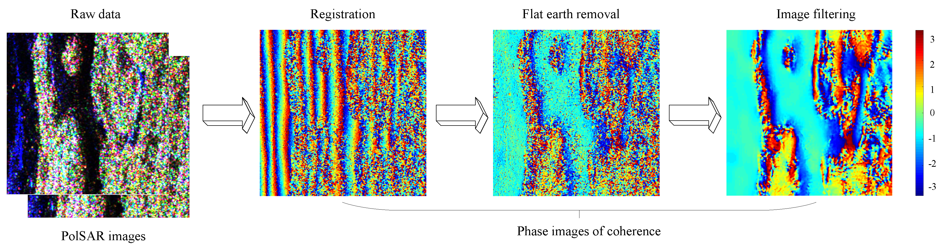
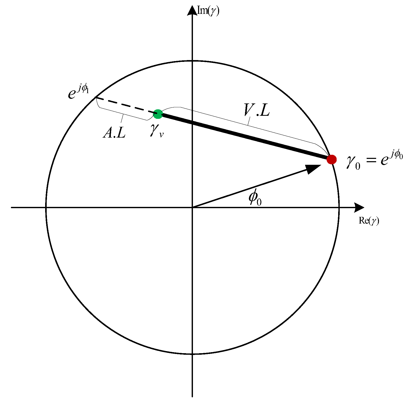
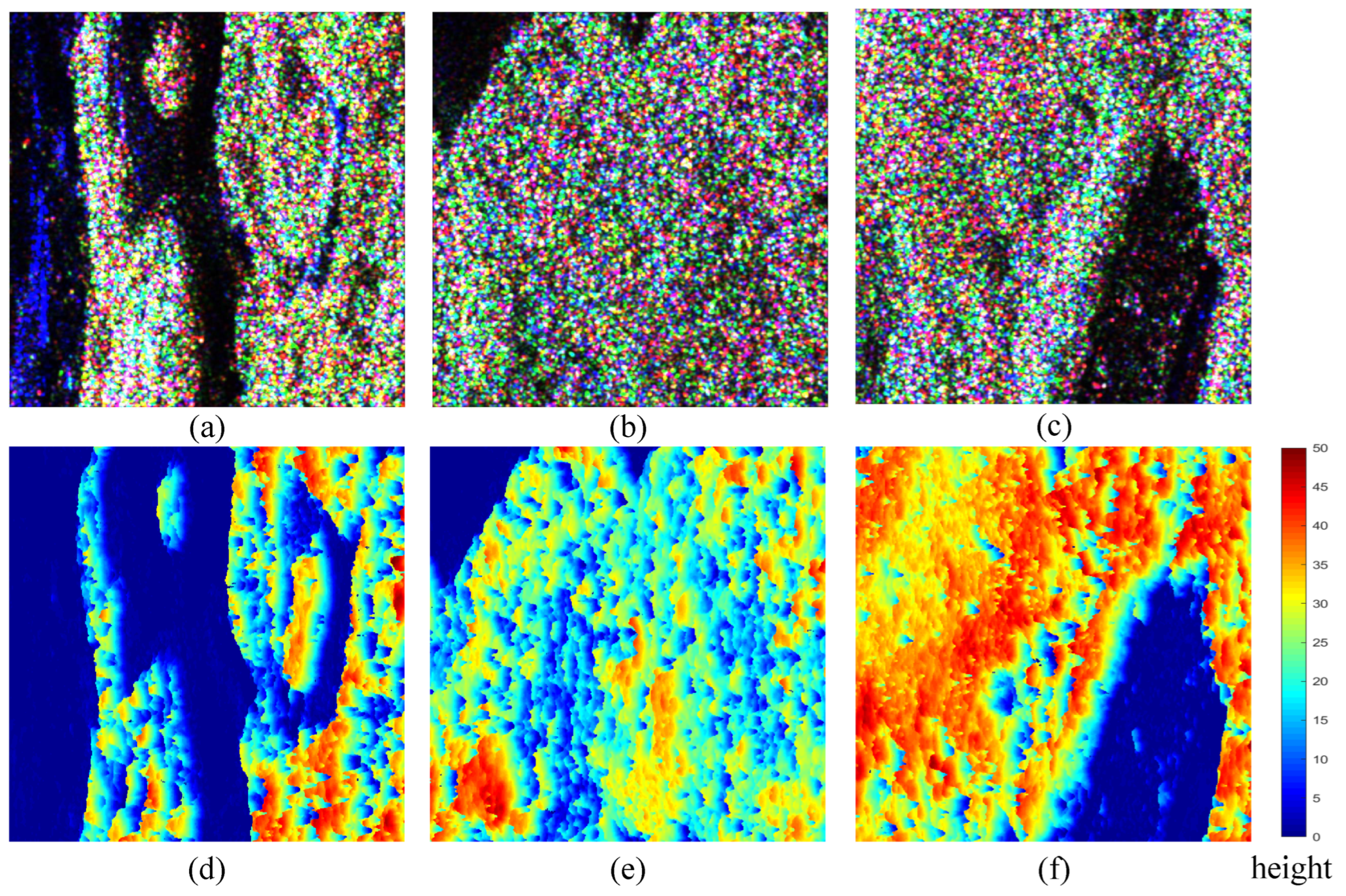