Assessing the Impact of Climate and Human Activities on Ecosystem Services in the Loess Plateau Ecological Screen, China

Abstract

The ecosystem services (ES) can be influenced by various environmental factors. In order to efficiently allocate resources and manage ecosystems, it is important to understand the mechanisms by which these environmental effects impact the interactions and trade-offs among different ES. While previous studies have primarily examined the impact of individual environmental factors on ES, the intricate mechanisms underlying the effects of multiple environmental factors have been largely overlooked. In this study, we adopted a path analysis approach that considered interactions among explanatory variables. We analyzed multiple geospatial datasets from various sources, including remote sensing and climate data, to examine the main drivers—precipitation, temperature, FVC (fractional vegetation cover), NPP (net primary productivity), human activities, and altitude—affecting five ecosystem services: carbon sequestration service (C), habitat provision service (HP), soil conservation service (SCS), sand-stabilization service (SSS), and water conservation service (WCS) in arid and semi-arid mountainous regions. Our investigation found that all five ES have shown an upward trajectory over the past two decades. The most significant growth was observed in C, which increased by 39.4%. Among the environmental factors examined, precipitation has been identified as the predominant factor influencing the ES and the synergies and trade-offs among ES. The influence of precipitation on SCS reached a coefficient of 0.726. Human activity factors had the greatest influence on HP of the five ES with a path coefficient of 0.262. Conversely, temperature exhibited a suppressive influence on ES. The impact of factors such as NPP and altitude on ES was comparatively modest. Notably, human activities assumed a substantial contributory role in shaping the relationship encompassing WCS. It is worth noting that individual factors exerted differential effects on ES along distinct environmental gradients, including anthropogenic gradients. In this context, the combination of high altitude and substantial FVC demonstrated a notable contribution to WCS. Our study can provide valuable insights for the management of ES which can be utilized to optimize the regulation of the Loess Plateau Ecological Screen (LPES) ecological construction and promote regional sustainable development.

1. Introduction

Ecosystem services (ES) refer to the various economic and social benefits that nature provides, such as landscape, culture, climate, energy, and materials. These services are essential for human well-being [1]. The exploration of ES synergies and trade-offs has become a prominent research topic in the field of ecology [2,3,4]. Considerable progress has been made in estimating ES, understanding their spatial patterns and temporal changes, and comprehending the interactions and trade-offs among multiple ES and associated risks [5,6,7,8,9,10,11,12]. Single-factor studies have broadly advanced our understanding of how individual environmental factors impact ES [13,14,15,16,17]. Ecosystem Services (ES) and their interconnections are shaped by ecological processes, influenced by several key environmental factors such as precipitation, temperature, FVC (fractional vegetation cover), NPP (net primary productivity), altitude, and human activities [18,19,20,21].

The LPES (Loess Plateau Ecological Screen) region encompasses altitudes ranging from 419 to 3590 m and is predominantly mountainous. Previous research has shown that environmental gradients, such as precipitation, altitude, and vegetation cover, have significant effects on ecosystem services in mountainous regions [22,23,24,25]. Research in the Qinling Mountains and other areas indicates that as elevation and vegetation cover increase, net primary productivity, soil conservation, and habitat quality also increase, while water yield and grain yield decrease [26]. Trade-offs between different ecosystem services exhibit varying sensitivities to changes in altitude, vegetation cover, and precipitation, with some increasing and others decreasing [27]. Mountainous areas often have higher biodiversity than surrounding lowlands due to the gradient effects of topography and climate [28]. Ma et al. [29] assessed the spatial variation of ecosystem services along a topographic gradient encompassing elevation, slope, topographic relief, and topographic ecotone. They proposed ecological management measures based on the vegetation types and characteristics of different topographic zones. However, despite the existing research on the response of ecosystem services to environmental gradients [30,31,32], these investigations frequently encounter two inherent limitations. Firstly, these studies often focus on only one factor, and studies that consider multiple factors fail to provide a comprehensive understanding of the primary drivers behind the response of ecosystem services to environmental gradients [22,26,27,28,29,30,31]. Secondly, the selection of influencing factors mainly focuses on natural factors, while the trade-offs associated with human activities are rarely explored [22,27,28,30,31,32]. Policymakers require a comprehensive understanding of the key factors that influence individual interests and trade-offs among multiple ecosystem services, especially when they may conflict with one another [33,34,35,36,37]. The intricate interplay and effects resulting from the combination of these multiple environmental factors on ecosystem services, along with their interconnectedness, have not been comprehensively grasped to sufficiently inform decision making in the context of LPES. Therefore, there is an urgent need for a fresh perspective and widely applicable analytical methods to consider the interactions between explanatory variables. These methods can help analyze the effects of environmental factors on ecosystem services and uncover relationships between different services [38,39]. By identifying the dominant factors and providing valuable insights, these methods will greatly enhance decision-making processes.

This study aims to quantify various ecosystem services in LPES by analyzing multi-source data from 2000 to 2020, considering the complex interplay between climate change, human activities, and ecosystem services. Techniques such as spatial correlation analysis, Pearson correlation coefficient method, and path analysis are employed to evaluate synergies, trade-offs, and the influence of environmental factors, like precipitation, temperature, fractional vegetation cover, net primary productivity, human activities, and altitude, on these services. This research aims to achieve the following objectives: (1) Determine the change patterns of ES in the LPES region over a 20-year period and identify synergies and trade-offs among them. (2) Identify the leading and inhibiting roles of environmental factors in the relationships among different ES. (3) Understand the complex influence of the gradient effects of environmental factors on ES. By clarifying the variation patterns of ES along these environmental gradients, this study intends to provide decision support for the management and planning of the LPES areas.

2. Study Area and Materials

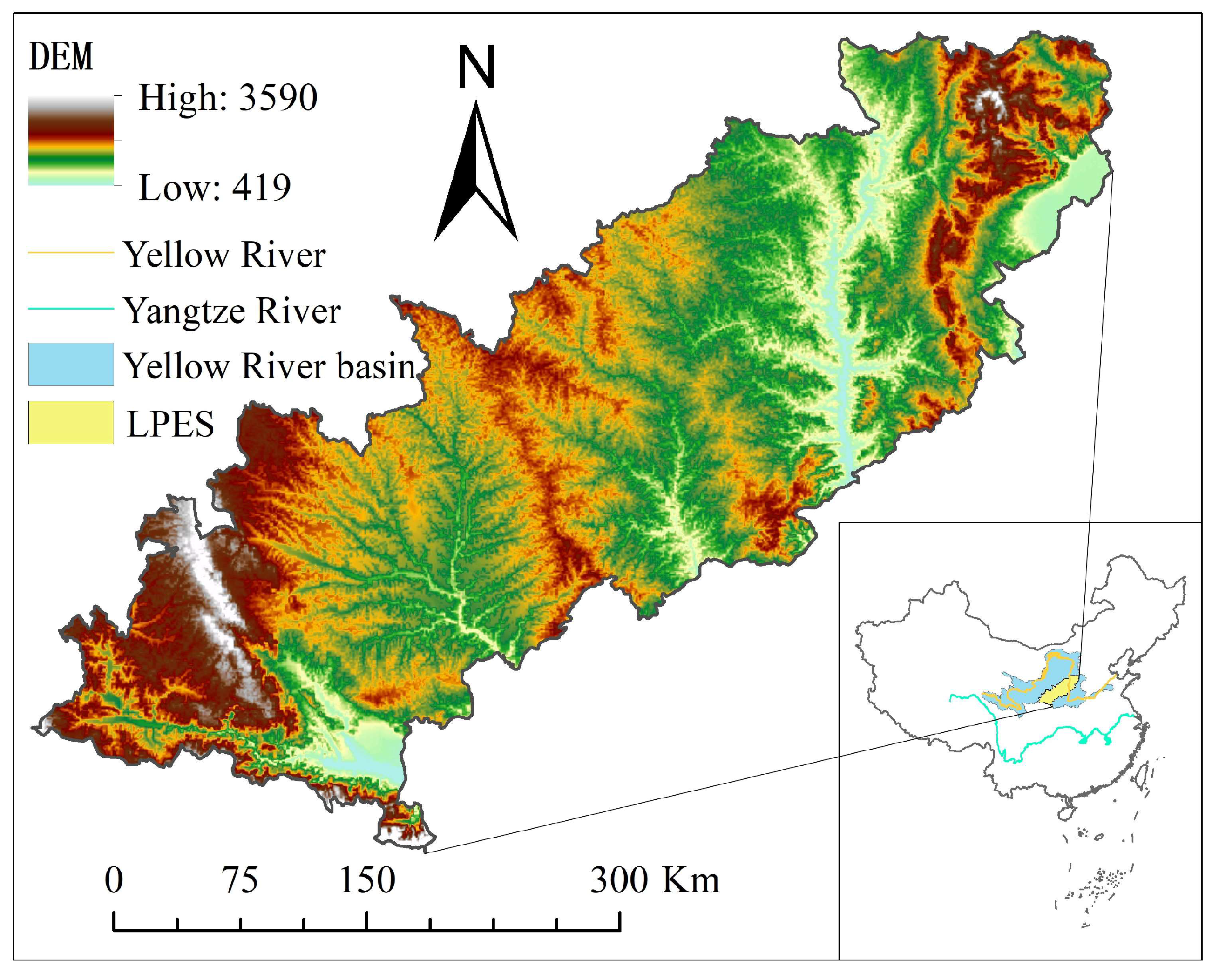
2.1. Study Area

The Loess Plateau Ecological Screen (LPES) is geographically situated between 105.1–112.21°E and 34.01–38.13°N in the middle section of the Yellow River. The LPES, extending from southwest to northeast in a strip-shaped configuration, covers an approximate area of 1.21 × 10⁵ km² (Figure 1). The altitude varies from 419 to 3590 m, with the highest elevation found in the southern Qinling Mountains. The topography of the Loess Plateau is marked by rolling hills and deep gullies. The region experiences an arid and semi-arid continental monsoon climate [40], with an average annual precipitation of around 600 mm, which is more abundant in the southeast and less in the northwest. The main forest ecosystem types are coniferous forest, mixed coniferous-broad forest, deciduous broad-leaved forest, sparse forest, evergreen broad-leaved scrub, deciduous broad-leaved scrub, open scrub, grassland, tussock, and meadow. The main land use patterns include agricultural, forestry, grassland, and construction use. Soil types include brown, gray-brown, loamy, black clay, loess, windswept, meadow, silt, swamp, and saline soils, to name a few [41]. The predominant soil type is loess with a loose structure, poor soil stability, and susceptibility to erosion. Precipitation in the LPES is concentrated in the summer months [42], generating large surface runoff, and the combination of fragile natural conditions and intensive long-term human activities has resulted in severe soil erosion [43]. The LPES is a vital part of the National Ecological Sheltering Zone, serving as an energy and mineral concentration area while also playing a crucial role in preventing desertification, controlling soil erosion, and protecting habitats [44].

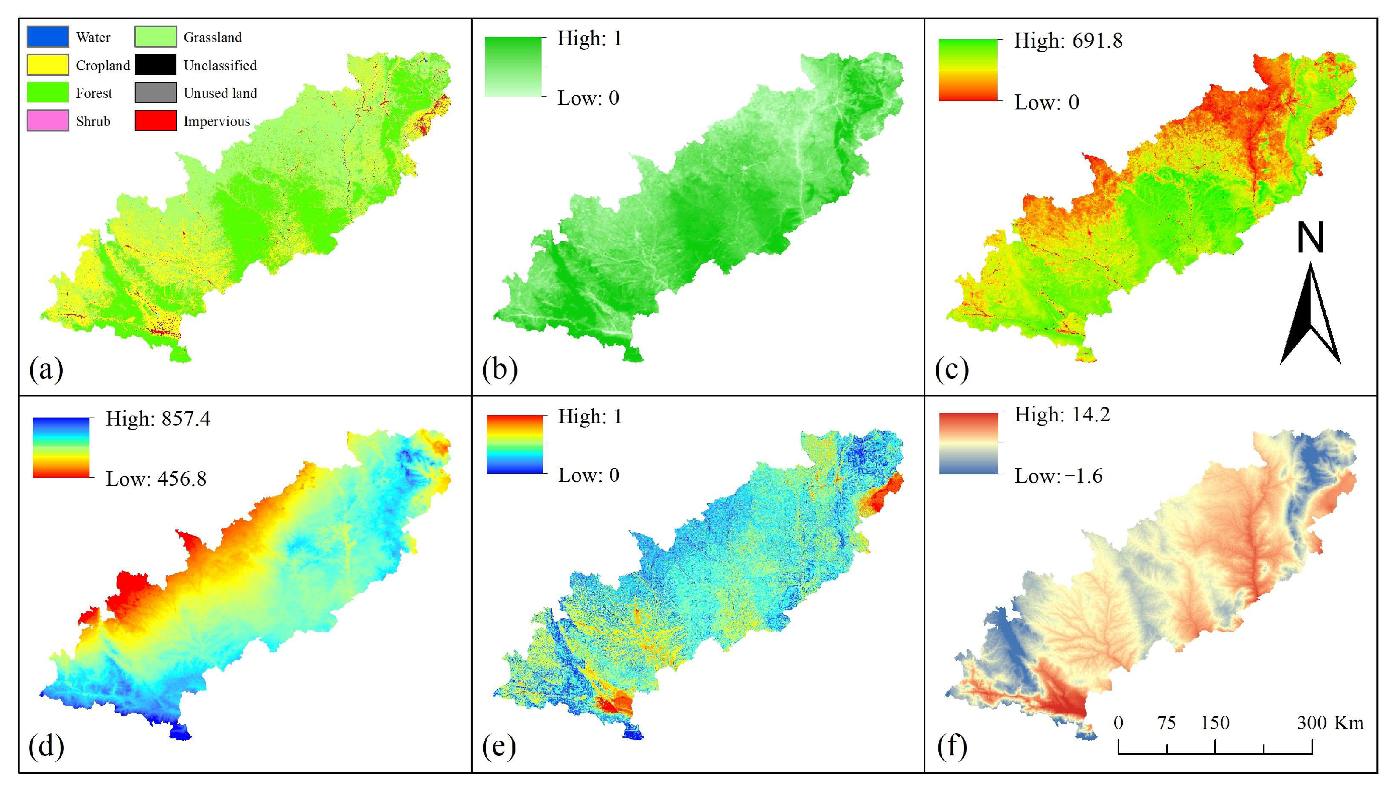
2.2. Data Source

The corresponding data sources are listed in

Table 1. Data source.

Name of Data	Data Source	Website	Resolution
Meteorological data (relative humidity, hours of sunshine, wind direction, wind speed, etc.)	China Meteorological Data Service Center	http://data.cma.cn (accessed on 1 September 2022)	Meteorological station data
LULC (land use and land cover) data	Chinese Academy of Science Resource Environment Science and Data Center	https://www.resdc.cn (accessed on 12 September 2022)	30 m
Population distribution data			1000 m
Temperature, precipitation, and evapotranspiration data	National Earth System Science Data Center and Loess Plateau Sub-Center	http://loess.geodata.cn (accessed on 15 September 2022)	1000 m
DEM (digital elevation model) data	Geospatial Data Cloud Site, Computer Network Information Center, and Chinese Academy of Sciences	http://www.gscloud.cn (accessed on 1 June 2022)	30 m
FVC (fractional vegetation cover) data and NPP (net primary productivity) data	National Aeronautics and Space Administration	https://ladsweb.nascom.nasa.gov (accessed on 15 June 2022)	250 m
Soil type data	National Soil Information Service Platform of China	http://www.soilinfo.cn (accessed on 10 June 2022	1000 m

. The meteorological station point data were converted into a raster format through kriging interpolation to cover the entire study area. The slope length and slope factor were derived from a 30 m DEM dataset. The calculation of SE involved data spanning from 2000 to 2020, with daily and monthly data aggregated into annual data for analysis. Other datasets used in the study are based on annual data specifically for the year 2020.

In order to facilitate research and calculations, as well as minimize the loss of accuracy caused by varying resolutions of raster data from different sources, the resampling technique in ArcGIS 10.8 was used in this research to normalize all the data to a consistent 500 m resolution. We recognized that when high-resolution data are resampled to lower resolutions, it can result in information loss and a decrease in detail, ultimately impacting the accuracy of the images [45]. To address this, we employed resampling methods, like Bilinear, Cubic Convolution, and Pixel Aggregate, to preserve the highest possible data quality. During the resampling process from high-resolution to low-resolution data, the nearest neighbor method ensured that the resulting high-resolution data did not introduce new values [46], while still enabling compatibility with other high-resolution datasets for overlay processing. By resampling the data to a relatively intermediate resolution, we aimed to minimize the loss of precision between the high- and low-resolution datasets. By referring to previous research [47,48,49,50,51], we conscientiously considered the unique characteristics of datasets with varying resolutions and implemented suitable resampling methods to strike a balance between accuracy and efficiency.

3. Methods

3.1. Ecosystem Services Valuation

3.1.1. Sand-Stabilization Service

The amount of wind erosion that would occur under the climatic conditions of an area, assuming no vegetation at all, is the potential wind erosion. The reduction in this wind erosion by the presence of vegetation is denoted as sand-stabilization service (SSS). This project uses the revised wind erosion equation (RWEQ) model [52,53,54] to estimate the sand-stabilization service in LPES. The calculation formula is shown below:

$$G=S_{\mathrm{L}1}-S_{\mathrm{L}2}$$

(1)

$$S_{\mathrm{L}1}=\frac{2·x}{{\left(150.71·EN{V}^{-0.3711}\right)}^2}·109.8·ENV·e^{-{\left(\frac{x}{150.71·EN{V}^{-0.3711}}\right)}^2}$$

(2)

$$S_{\mathrm{L}2}=\frac{2·x}{{\left(150.71{\left(ENV\times COG\right)}^{-0.3711}\right)}^2}·109.8\left[ENV\times COG\right]·e^{-{\left(\frac{x}{150.71{\left(ENV\times COG\right)}^{-0.3711}}\right)}^2}$$

(3)

$$ENV=AF\times EF\times SCF\times K^{\prime }$$

(4)

where, G indicates the quantity of sand fixation, kg/m²; $S_{\mathrm{L}1}$ and $S_{\mathrm{L}2}$ are the potential amount of wind erosion and the actual amount of wind erosion, kg/m²; x is the distance at which maximum wind erosion occurs, m; ENV is the environmental factor; AF for atmospheric factors, specific calculations refer to Gong et al. [55]; EF is soil erodibility factor; $SCF$ as soil surface cover factor (the calculation of EF and SCF is elucidated by Fryrear et al. [52]); K’ is the surface irregularity factor, obtained from the findings of Thomsen et al. [56]; COG is the vegetation cover factor.

(1) Atmospheric factor AF

Under natural conditions, the occurrence and development of wind erosion are driven or constrained by various meteorological conditions such as wind speed, temperature, precipitation, solar radiation, and snowfall. The atmospheric factor AF represents the comprehensive impact of various atmospheric factors on wind erosion, and its expression is as follows:

$$AF=Wf\times \frac{\rho }{g}\times SW\times SD$$

(5)

where, AF represents the meteorological factor, with units in kg/m; Wf is the wind force factor, with units in (m/s)³; ρ is the air density, with units in kg/m³; g is the gravitational acceleration, with units in m/s²; SW is the soil moisture factor, dimensionless; SD is the snow cover factor which, due to the lack of corresponding data, is set to 1 here.

(2) Soil moisture factor SW

Soil with higher moisture content is less susceptible to wind erosion, therefore, wind erosion is closely related to soil moisture. The soil moisture factor characterizes the amount of water content in the soil, which is a comprehensive reflection of regional precipitation and evaporation. Its expression is as follows:

$$SW=\frac{E{T}_p-\left(R+I\right)\left(R_d/N_d\right)}{E{T}_p}$$

(6)

$$E{T}_p=0.0162\frac{SR}{58.5}\left(DT+17.8\right)$$

(7)

where, R represents the average monthly precipitation, in mm; I is the irrigation amount; R_d is the average number of rainy days per month; N_d is the number of days per month; ET_p is the potential evaporation, in mm; SR is the average total solar radiation per month, in MJ; DT is the average temperature per month, in °C.

(3) Soil erodibility factor EF

The wind speed required to transport soil particles varies with their size, with coarser particles requiring higher shear wind speeds; when the required shear wind speed exceeds the actual wind speed, coarse soil particles will not be transported. Substances like organic matter, clay, and calcium carbonate in the soil can form micro-aggregates, reducing the soil’s erodibility. We have summarized Saleh’s experience and calculated the EF value using the following equation [57]:

$$EF=\frac{29.09+0.31sa+0.17si+0.33\left(\frac{sa}{cl}\right)-2.59OM-0.95cac{o}_3}{100}$$

(8)

where, sa represents the soil coarse sand content (%), si is the soil fine sand content (%), cl is the soil clay content (%), OM is the soil organic matter content (%), and caco₃ is the calcium carbonate content (%).

(4) Soil crust factor SCF

Soil particles, especially clay, silt, and organic matter particles, bond together to form a unique physical, chemical, and biological micro-layer on the soil surface, known as soil crust (also referred to as a crust layer). The calculation formula for the soil crust factor (SCF) is as follows:

$$SCF=\frac{1}{1+0.0066{\left(cl\right)}^2+0.021{\left(OM\right)}^2}$$

(9)

where, cl is the soil clay content (%) and OM is the soil organic matter content (%).

(5) Surface roughness factor K’

In RWEQ, surface roughness primarily refers to the changes in surface conditions and the impact on soil wind erosion due to the presence of cloddy soil and ridges produced by farming. Surface roughness is mainly calculated based on topography and slope.

(6) Vegetation cover factor COG

The vegetation cover factor indicates the extent to which vegetation inhibits wind erosion.

$$COG=e^{-0.0483\ast VC}$$

(10)

where, VC represents the vegetation cover degree (%).

3.1.2. Soil Conservation Service

Soil retention of vegetation is an indicator used to evaluate the benefits of land conservation, and it reflects the inhibitory effect of vegetation on soil erosion. Specifically, the soil retention of vegetation is equal to the potential soil erosion in the absence of vegetation minus the actual soil erosion that would have occurred with vegetation cover. The Universal Soil Loss Equation (USLE) is a model used to assess soil loss and is often utilized in large-area soil and water conservation studies in China. Therefore, USLE was selected to assess the soil conservation service (SCS) in LPES ecosystems for this project [58,59]. The calculation formula is shown below:

$$SC=S{E}_p-S{E}_a=R·K·LS·\left(1-COG\right)$$

(11)

where, $SC$ is the soil conservation, [t/(hm²·a)]; $S{E}_p$ and $S{E}_a$ are the potential soil erosion and actual soil erosion, respectively, [t/(hm²·a)]; $R$ is the precipitation erosion force factor, $\mathrm{MJ}·\mathrm{mm}/\left({\mathrm{hm}}^2·\mathrm{h}·\mathrm{a}\right)$, which is predicated upon the estimation of daily precipitation utilizing the semi-monthly precipitation erosivity model [60]; K is the soil erodibility factor, $\mathrm{t}·{\mathrm{hm}}^2·\mathrm{h}/\left({\mathrm{hm}}^2·\mathrm{MJ}·\mathrm{mm}\right)$, which was calculated using the EPIC model [61]; LS is the topography factor, calculated using the method of Nearing [62]; COG represents the vegetation cover factor, calculated using the method of Fistikoglu and Harmancioglu [63]. The calculation process for the different factors are shown below:

(1) Precipitation erosion force factor R

$$R={{\displaystyle \sum }}_{k=1}^{24}{\overline{R}}_k$$

(12)

$${\overline{R}}_k=\frac{1}{n}{{\displaystyle \sum }}_{i=1}^n{{\displaystyle \sum }}_{j=0}^m\left(\alpha ·P_{i,j,k}^{1.7265}\right)$$

(13)

$${\overline{R}}_k={{\displaystyle \sum }}_{k=1}^{24}{{\displaystyle \sum }}_{i=1}^n{{\displaystyle \sum }}_{j=0}^m\left(\alpha ·P_{i,j,k}^{1.7265}\right)$$

(14)

where, R is the multi-year average annual precipitation erosion force, $\mathrm{MJ}·\mathrm{mm}/\left({\mathrm{hm}}^2·\mathrm{h}·\mathrm{a}\right)$; ${\overline{R}}_k$ is semi-monthly, where k is the precipitation erosion force of the k-th semi-month, $\mathrm{MJ}·\mathrm{mm}/\left({\mathrm{hm}}^2·\mathrm{h}·\mathrm{a}\right)$ for 24 and a half months of the year, i.e., k = 1, 2, …, 24; i is the year of the used precipitation information, i.e., i = 1, 2, …, n; j is the number of days of erosive precipitation in the k-th half month of the i-th year, i.e., j = 1, 2, …, m; $P_{i,j,k}$ is the j-th erosive daily precipitation in the k-th half month of the i-th year (mm); $\alpha$ is a parameter with $\alpha$ = 0.3937 in the warm season and $\alpha$ = 0.3101 in the cold season.

(2) Soil erodibility factor K

$$K=\left(-0.01383+0.51575·K_{EPIC}\right)$$

(15)

$$\begin{gathered} K_{EPIC}=\left\{0.2+0.3·e^{\left[-0.0256·m_s\left(1-m_{silt}/100\right)\right]}\right\}\times {\left[m_{silt}/\left(m_c+m_{silt}\right)\right]}^{0.3}\times \left\{1-0.25·orgC/\left[orgC+ \\ {e}^{\left(3.72-2.995·orgC\right)}\right]\right\}\times \left\{1-0.7\left(1-\frac{m_s}{100}\right)/\left\{\left(1-\frac{m_s}{100}\right)+e^{\left[-5.51+22.9\left(1-\frac{m_s}{100}\right)\right]}\right\}\right\} \end{gathered}$$

(16)

where, $m_c$, $m_{silt}$, $m_s$, and $orgC$ are the clay grain (<0.002 mm), powder grain (0.002~0.05 mm), sand grain (0.05~2 mm) and organic carbon, %, respectively.

(3) Topographic factors LS

$$L={\left(\lambda /2.13\right)}^m$$

(17)

$$S=\left\{\begin{array}{c}\begin{array}{c}10.8\sin \theta +0.03 \theta <5.14°\\ 16.8\sin \theta -0.5 5.14°\le \theta <10.20°\end{array}\\ 21.91\sin \theta +0.96 10.20°\le \theta <28.81°\\ 9.5988 \theta >28.81°\end{array}\right.$$

(18)

where, L is the slope length factor; S is the slope factor; m is the slope length index; $\theta$ is the slope, °; $\lambda$ is the slope length, m.

3.1.3. Water Conservation Service

The water balance equation was used for the calculations, where water supply services are assumed to be equal to the difference of precipitation minus evapotranspiration and stormwater runoff. The calculation of evapotranspiration is based on the Zhang model [64], while stormwater runoff is estimated using the stormwater production model. The calculation indexes include annual precipitation, annual evapotranspiration, and annual precipitation runoff. The water balance equation is calculated as follows:

$$WB=PREP-ET-QF$$

(19)

where, WB is the water-bearing capacity, mm; PREP is the annual precipitation, mm; QF is the stormwater runoff, mm; ET is the actual evapotranspiration, mm.

(1) Stormwater runoff QF

Stormwater runoff is calculated using precipitation multiplied by runoff coefficients, where the extent to which different land use types respond to precipitation varies.

$$QF=P\times \alpha$$

(20)

where, P is precipitation, mm; α is the surface runoff coefficient for different land use/cover types (

Table 2. Surface runoff coefficients for different grassland types.

Forest and Grassland Ecosystem Type	α
coniferous forest	3.02
mixed coniferous-broad forest	2.29
deciduous broad-leaved forest	1.33
sparse forest	19.2
evergreen broad-leaved scrub	4.26
deciduous broad-leaved scrub	4.17
open scrub	19.2
grassland	4.78
tussock	9.37
meadow	8.2

).

3.1.4. Carbon Sequestration Service

The carbon sequestration service (C) is calculated by multiplying the biomass of various vegetated ecosystems with the corresponding biomass–carbon conversion coefficients. These coefficients are determined using techniques such as quantitative remote sensing of vegetation, model fitting, and actual sample plot data [65,66,67,68,69,70,71]. The main calculation formula is as follows:

$$COS={{\displaystyle \sum }}_{i=1}^{j}AG{B}_i\times C_i$$

(21)

where, COS is the amount of carbon stored in the vegetation and other aboveground biomass within terrestrial ecosystems; i is the i-th type of ecosystem; j is the overall quantity of distinct ecosystem categories; AGB_i is the aboveground biomass of the i-th ecosystem type; the coefficient C_i represents the amount of carbon produced from the biomass of ecosystem type i.

3.1.5. Habitat Provision

The evaluation of regional biodiversity in this project, which focused on regional habitat quality and habitat scarcity, was based on calculations performed using the InVEST model (Stanford University, Stanford, CA, USA, model available at https://naturalcapitalproject.stanford.edu/software/invest, accessed on 1 May 2022), as evidenced by the biological habitat quality index [72,73,74,75,76,77,78]. More details can be found in the InVEST user’s guide (https://storage.googleapis.com/releases.naturalcapitalproject.org/invest-userguide/latest/en/index.html, accessed on 1 May 2022) and the relevant literature [79,80]. The calculation formula is as follows:

①

site quality

$$D_{xj}={{\displaystyle \sum }}_{r=1}^R{{\displaystyle \sum }}_{y=1}^{Y_r}{r}_y{i}_{rxy}{\beta }_x{S}_{jr}\left(\frac{w_r}{{{\displaystyle \sum }}_{r=1}^R{w}_r}\right)$$

(22)

where, $D_{xj}$ is the total stress level of raster x in LULC (land use and land cover) or habitat type j; $r_y$ is the stress factor in raster; y is the stress effect of the stress factor in raster on raster, and the stress effect is divided into linear decay and exponential decay; the impact of stress factor r on raster y in raster x is represented by $i_{rxy}$, and this impact is categorized into two types of stress effects: linear decay and exponential decay; ${\beta }_x$ is the reachability level of raster x; $S_{jr}$ is the sensitivity of habitat type j to stress factor r, (if $S_{jr}$ = 0, then $D_{xj}$ is not a function of threat r); the weight assigned to a stressor is known as $w_r$ and reflects the extent of the damage caused by that stressor on all types of habitats.

②

habitat scarcity

$$R_x={{\displaystyle \sum }}_{x=1}^X{\sigma }_{xy}\left(1-\frac{N_j}{N_{jbaseline}}\right)$$

(23)

where, $R_x$ is the scarcity of raster x; $N_j$. $N_{jbaseline}$ is the number of LULC (land use and land cover) type j grids in the baseline landscape pattern; ${\sigma }_{xy}$ is a binary number, ${\sigma }_{xy}$ = 1 when raster x is of LULC (land use and land cover) type j, otherwise ${\sigma }_{xy}$ is 0.

3.2. Ecosystem Services Trade-Offs and Synergies

Synergy: when the enhancement of one service is carried out together with the enhancement of another service, there is synergy between the two services [81]. Trade-off: a trade-off between two ecosystem services occurs when one service is promoted at the sacrifice of the other [82]. Unrelated: if one ecosystem service increases or remains unchanged while the other does not change, then their interaction is considered unrelated. In each sub-barrier, there is spatial heterogeneity among various ecosystem services, which can result in localized trade-offs and synergies due to the unique spatial distribution patterns [10,83,84,85]. Therefore, the correlation coefficients between the five ES in the study area for the five periods from 2000 to 2020 were calculated using the image-by-image spatio-temporal correlation analysis.

The correlation coefficients between the two groups of ecosystem services were calculated separately based on the image-by-image spatial correlation analysis method—Pearson product–moment correlation coefficient method [86]. The trade-offs and synergies between ecosystem services are measured according to the positive and negative correlation coefficients and the magnitude of the absolute value of the relationship with the following equation:

$$R=\frac{\sum \left(x_i-\overline{x}\right)\sum \left(y_i-\overline{y}\right)}{\sqrt{\sum {\left(x_i-\overline{x}\right)}^2\sum {\left(y_i-\overline{y}\right)}^2}}$$

(24)

where, R is the correlation coefficient; if R is positive, the relationship between the two services is synergistic, and vice versa, the relationship is a trade-off; if R is 0, there is no correlation, and a larger absolute value indicates a stronger correlation, i.e., a greater degree of synergy or trade-off; x and y are the two ecosystem service variables; i is the data of the i-th period.

3.3. Construction of an Evaluation System for Assessing the Impact of Human Activities

Rapid socioeconomic development drives an increased demand for natural resources, leading to intensified and widespread human activities that transform the natural environment. Consequently, this results in escalating disturbances and pressures on the ecological environment [87,88,89]. When assessing their impact on the ecological environment, one widely used approach involves analyzing LULC changes, which serve as a direct and prominent indicator of human activities on the surface ecosystem. Evaluating regional human activity intensity from a landscape perspective through LULC changes is a common and effective method [90,91,92]. The research conducted by Yang et al. [93] demonstrates that rural settlements increasingly exhibit a pronounced tendency to cluster and develop in areas characterized by superior topographic conditions, particularly those with lower gradients. So, we included the terrain factor in evaluating the intensity of human activities and discovered that population density is directly related to human activity [94,95].

In this study, a total of five indicators, including altitude, slope, undulation, LULC, and population density index, were selected to construct an evaluation system of human activity intensity. In this study, the final human activity intensity was calculated by the ArcGIS spatial statistics method using weighted summation. The calculation formula is below:

$$T_i={{\displaystyle \sum }}_{i=1}^n{W}_i\times C_i$$

(25)

where, T represents the composite score of the human activities index of each evaluation unit within the raw LPES, n represents the i-th evaluation index factor, C_i corresponds to the score of the i index factor, and W_i represents the weight of the corresponding i index factor.

According to the actual LPES [96,97,98,99], an expert scoring method was used to assign indicator values to each category of indicators (

Table 3. Human activity intensity evaluation system.

Evaluation Index Factors	Weights	Classification	Score
Altitude (m)	0.1	419–800	100
		800–1200	60
		1200–1600	30
		>1600	10
Undulation (m)	0.1	0–60	100
		60–120	80
		120–180	50
		>180	10
Slope (°)	0.1	0–3°	100
		3–6°	75
		6–9°	50
		>9°	25
LULC (land use andland cover)	0.2	Unclassified	0
		Cropland	80
		Forest	40
		Shrubs	20
		Grassland	10
		Waters	5
		Unused land	0
		Impervious	100
Population density	0.5	13–3222 people/Km2	13 people/Km2 0 3222 people/Km2 100

).

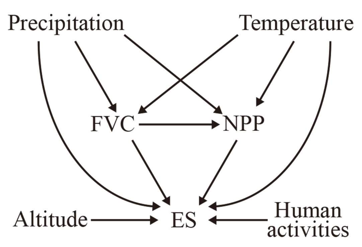
3.4. Path Analysis

Passage path analysis is a multi-variate statistical analysis technique that belongs to the Structural Equation Model (SEM) [100]. Unlike typical statistical techniques such as simple or multiple regression, path analysis facilitates the exact quantification of associations among numerous independent and dependent variables. Further, it distinguishes between the direct and indirect effects of the explanatory variables on the response variable. To conduct a path analysis, a conceptual model must first be built, employing our a priori knowledge about empirical connections between variables [101]. In this study, we developed a conceptual model specifying the relationship between different factors and ES, while considering the interactions between these factors (see Figure 2). Specifically, we hypothesized that the six factors, precipitation, temperature, FVC, NPP, human activities, and altitude, affect ES not only directly, but also indirectly through the interactions among these factors. Each of the paths we hypothesized has been studied by scholars. For example, temperature to FVC, NPP [102,103,104,105,106]; precipitation to FVC, NPP [107,108]; FVC to NPP [109]; human activities to ES [110]; FVC to ES [111,112,113]; temperature to ES [114]; precipitation to ES [112,115,116]; altitude to ES [117], etc. We quantified the effect of explanatory variables on response variables using standardized path coefficients. For example, the total impact of precipitation on ES is calculated as the sum of the products of the normalized path coefficients along each path from precipitation to ES. In this study, a path analysis of the effects of each factor on ES was conducted, followed by a path analysis of the effects of synergies and trade-offs between the factors on ES. Finally, in ArcGIS 10.8 software, the spatial coordinates of the six different environmental factors from various data sources were standardized. The raster data were then resampled to a resolution of 500 m, ensuring that all raster data had the same number of rows and columns. Then, using the equal interval method, the six factors were divided into four equal-value gradients, and the impact of each factor on ES under different gradients was investigated (Figure 3 and Figure 4). The path analysis was performed in R using the “lavaan 0.6-12” package and all variables were normalized prior to the analysis [118]. The normalization method is shown in Equation (26):

$$X^{\ast }=\left(X-min\right)/\left(max-min\right)$$

(26)

where, max is the maximum value of raster data and min is the minimum value of raster data.

4. Results

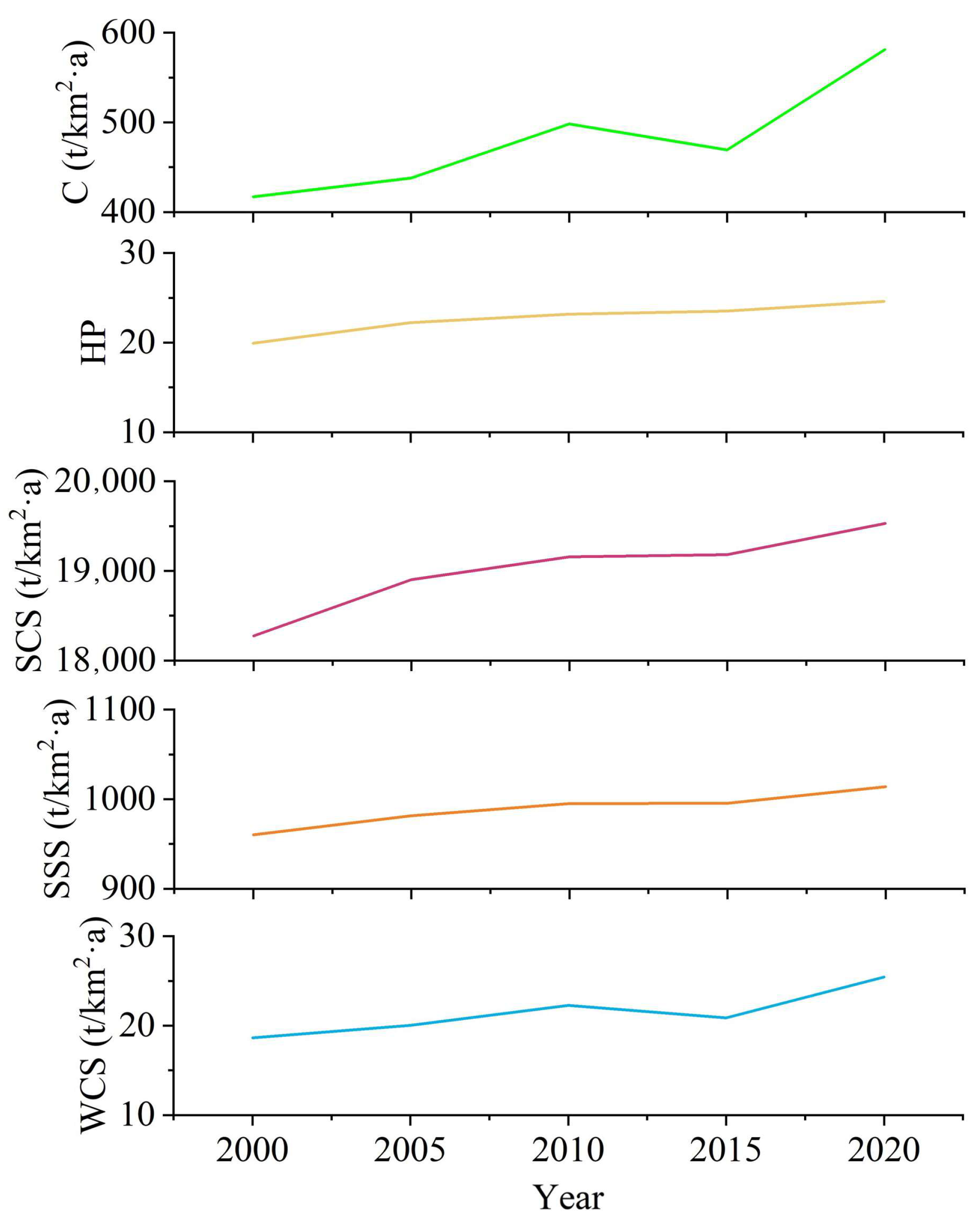
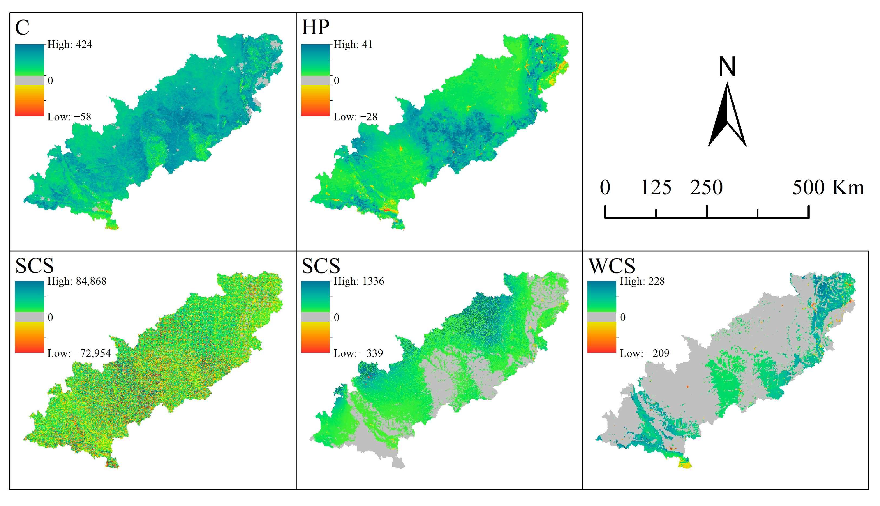
4.1. Trends in ES on the Loess Plateau Ecological Screen from 2000 to 2020

Over the 20 years, the five ES values have been in a fluctuating upward trend (Figure 5). The most significant growth was seen in C (carbon sequestration service), with an increase of 39.4%, while SSS (sand-stabilization service) grew more slowly, with an increase of 5.6%. WCS (water conservation service) increased by 36.4%, HP (habitat provision service) by 23.5%, and SCS (soil conservation service) by 6.9%. With the exception of HP, there were significant fluctuations in the other four ES in 2015.

Figure 6 reveals that C and HP are increasing across most areas, with only a small portion showing a decline in impervious land use types. Approximately one-third of SSS exhibits non-growth, largely coinciding with forest distribution. Conversely, WCS demonstrates non-increasing trends in around two-thirds of the area, with areas of growth highly overlapping with forest distribution. The growth and decrease in SCS exhibit irregular patterns. Overall, the ecosystem services in the LPES region show a positive trend of increase.

4.2. Ecosystem Service Trade-Offs and Synergies

See Figure 7. There was a high synergy between HP and SSS throughout the study area; however, due to the absence of SSS growth in forested regions, HP and SSS are not correlated in forested distribution areas. The co-increase in HP and SSS is likely due to the combined effect of vegetation structure. Complex vegetation structures can provide the habitat diversity and food chain support required by habitats [119,120]. A more complex vegetation structure can slow down wind speed and reduce wind erosion of the soil [121]. HP and SSS are the most obvious synergy of the ten relationships. The HP and SSS trade-offs were mainly distributed in the impervious region. The high synergy and high trade-off between SCS and SSS were interleaved in the distribution, and again, SCS and SSS were uncorrelated in forested areas. C and SSS had significant trade-offs in grasslands in the northern region, with high overlap with areas of low NPP values, high synergy values in the south and the east where cropland intersected with impervious land and grasslands, and low synergy interspersed with low trade-off values in the rest of the region. Due to the significant presence of non-changing regions in both WCS and SSS data, these areas complemented each other within the study area. As a result, the uncorrelated regions of WCS and SSS were the largest in extent. The synergy between SCS and HP was more pronounced in the steppe region, while other regions exhibited a combination of high synergy and high trade-offs. The areas with higher trade-off values of C and HP aligned with the lower values of NPP, whereas the regions with higher synergy values were found in lower elevation areas. The high synergy between WCS and HP was distributed in the forest region, as WCS changed only in the forest region, and only a few of the low trade-offs were distributed in the southernmost high-altitude areas of the study area. In the northern part of the study area, there was a more concentrated trade-off between C and SCS, particularly in regions with low NPP values. The distribution of WCS and SCS was similar to that of WCS and HP, but the relationship was mainly low synergy and low trade-off. Similarly, the distribution of WCS and C showed a resemblance to WCS and HP, with the relationship primarily being a trade-off, except in high precipitation areas in the southern part of the study area where synergy was observed.

4.3. Ecosystem Services Impact Factor

We used path analysis to assess the relative effects of precipitation, temperature, FVC, NPP, human activities, and altitude on ES and to determine which of the six factors best explained the synergy and trade-offs of ES. In the model, all six factors were considered to affect ES directly, precipitation, and temperature were considered to affect ES indirectly through FVC and NPP, and FVC indirectly through NPP (Figure 8).

Precipitation had a larger total effect on C (net effect = 0.699) than FVC, human activities, and altitude (net effects of 0.165, 0.098, and 0.08, respectively), with NPP and temperature acting as inhibitors of C (net effects of −0.045 and −0.152). Precipitation had a larger total effect on HP (net effect = 0.594) than FVC, human activities, altitude, and temperature (net effects of 0.16, 0.262, 0.271, and 0.082, respectively), with NPP acting as a suppressor of HP (net effect of −0.015). Precipitation had the largest total effect on SCS (net effect = 0.726), which was greater than FVC, human activities, and altitude (net effects of 0.183, 0.151, and 0.071, respectively), where temperature and NPP played an inhibitory role on SCS (net effects of −0.095 and −0.019). Precipitation had the most significant overall effect on SSS with a net effect value of 0.675, compared to FVC and human activities, which were inferior to precipitation in terms of their net effect on the ecosystem. Specifically, the net effect of FVC was 0.136 and the net effect of human activities was 0.148. The net benefit of NPP on SSS was −0.063, and when ecosystem NPP increases, it may not necessarily have a positive impact on ecosystem maintenance and development but may instead have a degree of inhibitory effect. The net effect of temperature on SSS was −0.103, which implies that an increase in temperature may have a negative effect on SSS. Precipitation had the largest total effect on WCS (net effect = 0.707), which was greater than FVC, human activities, and altitude, (net effects of 0.101, 0.092, and 0.175, respectively). Temperature and NPP inhibited SCS (net effect of −0.101 and −0.012, respectively). In conclusion, precipitation has a significant impact on various ecosystem indicators and, in many cases, its influence is more pronounced compared to other factors. These findings highlight the crucial role of precipitation in maintaining and shaping ecosystem functionality. The findings from Wang et al.’s [122] study further support that water yield in the Loess Plateau region is primarily influenced by annual mean precipitation, which emerges as the dominant driving factor.

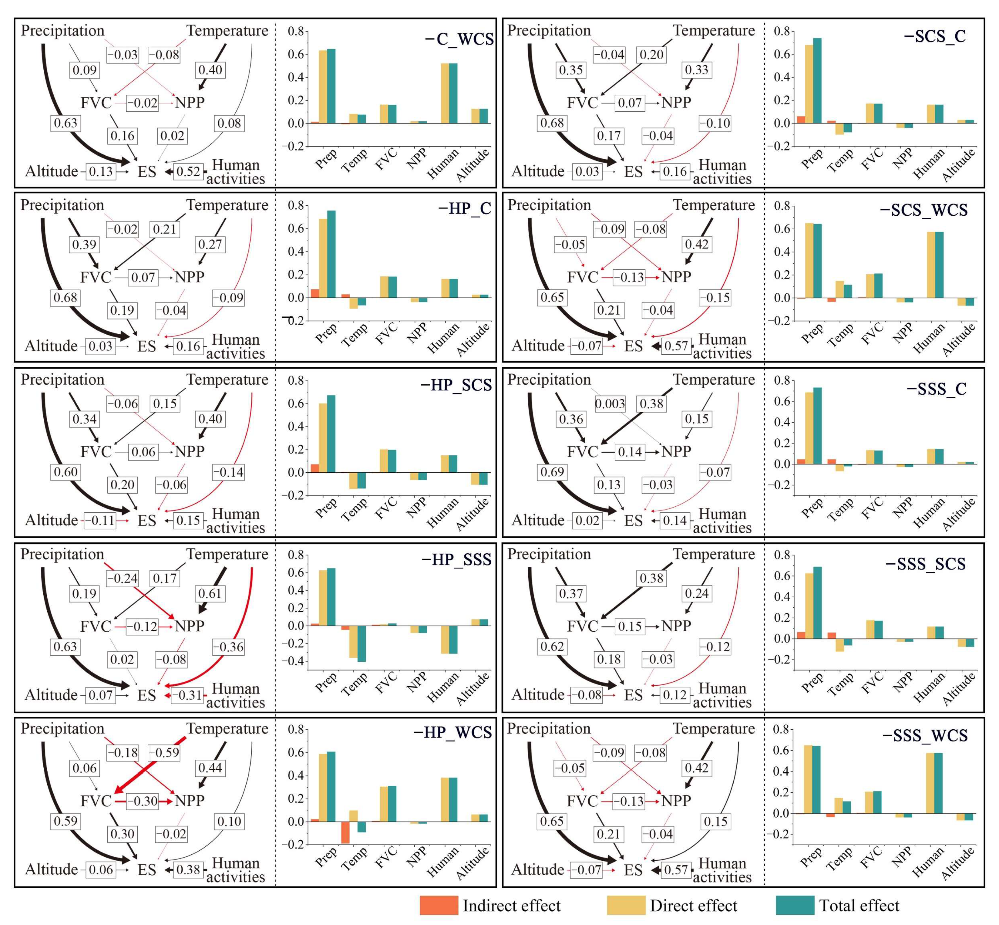
4.4. Ecosystem Service Trade-Offs Impact Factor

Among the trade-offs among ecosystem services, the total effect of precipitation on ES was dominant and played a facilitating role (Figure 9). The direct effect of precipitation on both HP and C and SCS and C was 0.68. In the relationship where both contain C, it is possible that precipitation promotes C and inhibits HP and SCS. The net benefits of human activities on the trade-offs between SCS and WCS, SSS and WCS, and C and WCS are 0.573, 0.573, and 0.521, respectively, indicating that the impact of human activities will cause SCS, SSS, and C to grow at the expense of a portion of WCS. Temperature exerted a significant inhibitory effect on the trade-off between HP and SSS, with a direct effect of −0.36.

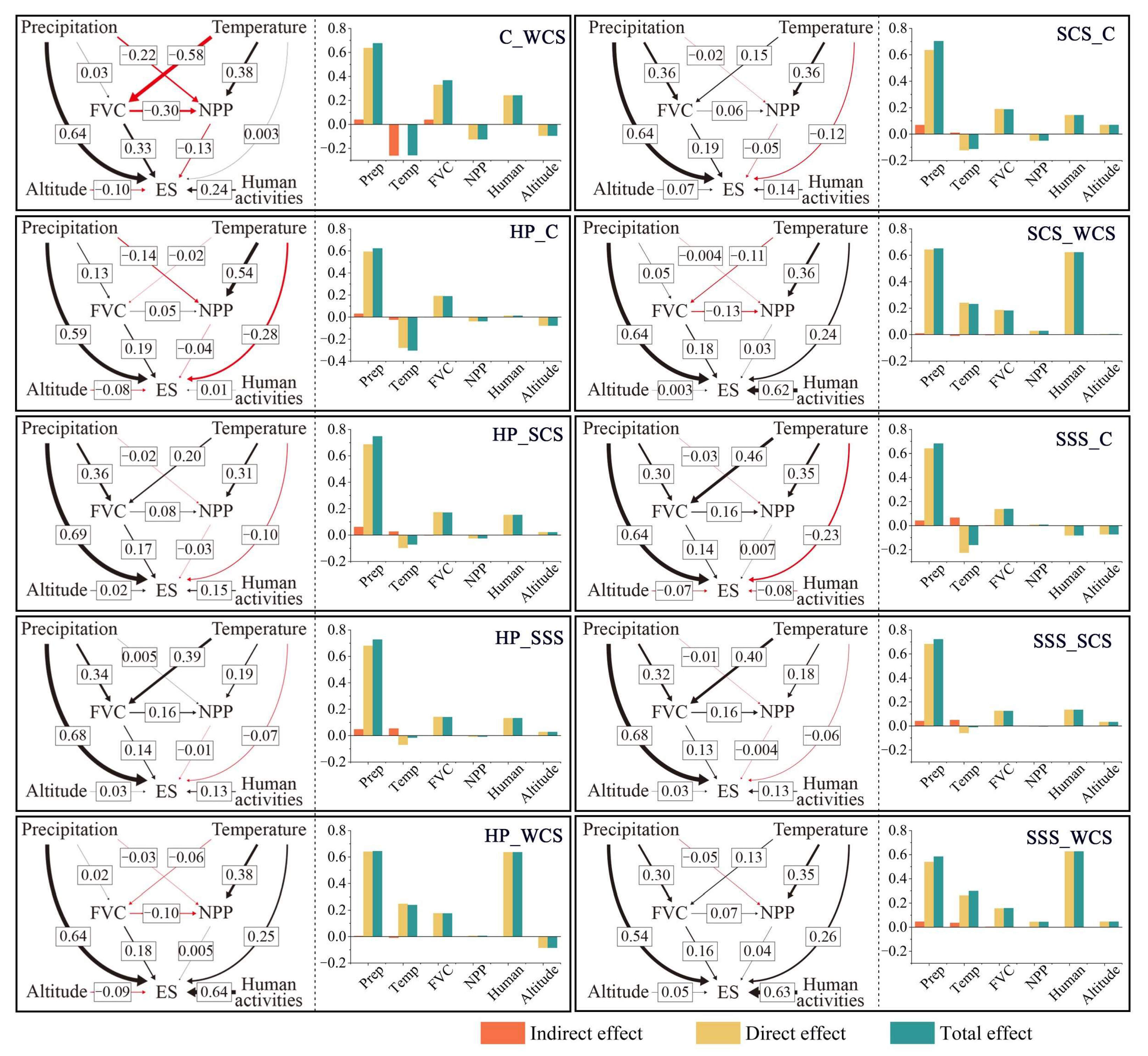
4.5. Ecosystem Services Synergies Impact Factor

See Figure 10. In the synergy of C and WCS, precipitation is the main influencing factor of the relationship with a net benefit of 0.676, of which the direct benefit is 0.64, the effect on ES synergy through FVC is only 0.03, and the effect through NPP is −0.22. Temperature has negligible direct effects on the synergy between C and WCS (0.003). However, its indirect effect through FVC (−0.58) is more apparent, as indicated by the path coefficient analysis. This suggests that temperature indirectly inhibits synergy by negatively influencing FVC. Human activities and FVC contribute to the synergy of C and WCS, while altitude and NPP act as inhibitors. Notably, FVC inhibits the inhibitory effect of NPP by inhibiting NPP and thus, the indirect effect of FVC on the synergy of C and WCS is also facilitated. In the synergy of HP and C, precipitation is the main influencing factor of the relationship with a net benefit of 0.623, where the direct benefit is 0.59 and the net effect of FVC is 0.189. The temperature factor indirectly inhibits ES synergy through a strong facilitative effect on NPP, which, together with the direct inhibitory effect of −0.28, results in a total effect of −0.303. The relationship between the effects of several other factors is weaker. The dominant factors of HP and SCS are similar to HP and C, but the temperature factor promotes the synergy of HP and SCS through to FVC. The dominant factors for HP and SSS are similar to those for HP and SSS, but the contribution of temperature to FVC is more pronounced, with an effect coefficient of 0.39 for this path. The role of human activities is noteworthy across multiple synergies. It is evident that human activities significantly contribute to the synergies of HP and WCS, SCS and WCS, and SSS and WCS. This contribution is comparable to the net benefit of precipitation, underscoring the importance of human activity in shaping these relationships. All three relationships involve WCS. Earlier, we hypothesized that planted forests could respond to human activities to some extent. A study conducted by Jin et al. [123] demonstrated that planted forests in the Loess Plateau region have the potential to enhance soil water-holding capacity and improve water retention abilities. The contribution of altitude and NPP factors in all ten synergies was relatively weak, and the effect of the altitude factor was almost negligible in the relationship between SCS and WCS. The effect of the NPP factor was also negligible in the synergy of HP and WCS, SSS and C, and SSS and SCS. In the synergy of SSS and WCS, only precipitation was inhibitory to NPP, while the rest were facilitative.

5. Discussion

5.1. Analysis of the Individual Drivers of Ecosystem Services

In this study, a path analysis model was utilized to analyze the direct and indirect effects of different factors on ecosystem services (ES). The findings indicate that the dominant factors influencing ES are consistent in LPES, where precipitation plays a significant role in explaining the variation in ES, while the impact of NPP on ES is relatively weak. Precipitation plays a crucial role in supporting vegetation growth as it acts as a necessary condition. In arid and semi-arid regions, precipitation plays a crucial role in promoting vegetation growth and directly impacting its condition. When analyzing the direct path of ecosystem services (ES) without dividing the gradient, the path coefficient from precipitation to FVC is approximately 0.35. Similarly, when assessing synergies and trade-offs between ES, this path coefficient from precipitation to FVC is often around 0.30. It is worth noting that only the trade-offs among SSS, SCS, and WCS exhibit negative values for this path coefficient from precipitation to FVC. This can be attributed to precipitation promoting all three ES and thus suppressing the trade-offs between them. Given that the response of each ES to climatic factors is a shared response, it becomes challenging to elucidate the specific impact of individual climatic factors on their relationship with ES [124]. For example, precipitation can modulate the extent of SCS by affecting changes in surface runoff [125]. Research has demonstrated that warming expedites the decomposition of soil organic matter and extends the vegetation growth period, thereby facilitating vegetation growth [105]. Therefore, in a direct study of ES, this coefficient of passage from temperature to NPP is 0.35. It is also common for this coefficient of passage from temperature to NPP to be greater than 0.40 in a pathway analysis of synergies and trade-offs among ecosystem services. Temperature is a major factor affecting NPP. Temperature directly or indirectly influences physiological processes such as photosynthesis, respiration, and plant water transpiration, which in turn impact the magnitude of NPP. More specifically, as temperature rises, the rate of photosynthesis tends to increase at a faster rate compared to the acceleration in plant respiration. This dynamic effect leads to a promotion of the net photosynthetic rate, thereby facilitating an overall increase in the plant’s productivity. Simultaneously, an elevation in temperature also results in an upsurge in the transpiration rate of plant leaves, thereby influencing plant water use efficiency. According to Zhu et al. [106], a significant decrease in summer temperatures within the central Loess Plateau may have detrimental effects on vegetation growth. Overall, the promotion effect of temperature on NPP is more significant within a certain range, but beyond the plant physiological adaptation zone, plant growth is inhibited, thus reducing NPP [102,103,104].

Agricultural activities, industrial production, and other human endeavors necessitate significant amounts of water resources. However, the wastewater and industrial waste stemming from such activities can contaminate neighboring water sources, thereby posing a threat to the quality and stability of the watershed ecosystem [126,127]. Thus, human activities exacerbate the four trade-offs between WCS and HP, C, SSS, and SCS. However, we observed a similar pattern in terms of synergy, where the net benefits of human activities for C and WCS, HP and WCS, SCS and WCS, SSS and WCS were 0.241, 0.636, 0.622, and 0.626, respectively. Among these relationships, only C and WCS demonstrated lower values for the path coefficient influenced by human activities. The Chinese government’s implementation of the “Three-North Shelter Forest Program” in recent years has generally resulted in a promotion of C. However, the promotion of WCS in areas with significant human activities is not as pronounced as it is for C. It is worth mentioning that the relationship between C and WCS is not as explicitly influenced by human activities compared to the other three factors.

In the NPP gradient, the effect of the altitude factor on C gradually diminished with increasing NPP, and at NPP values above 518.8 (at normalized values greater than 0.75) the altitude factor exerted an inhibitory effect on C (Figure 11 (1)). Li et al. [128] demonstrated a negative correlation between aboveground biomass carbon density and altitude in the Loess Plateau. At LPES, higher altitude results in greater diurnal temperature differences. In areas with lower NPP values, plants experience less spatial competition pressure and higher diurnal temperature differences can enhance plant carbon accumulation. This finding is similar to Warren’s conclusion that increasing altitude has a positive effect on the reproduction of understory plants [129]. In human activities, the temperature factor decreased and then increased with increasing NPP gradient for ES, while the precipitation factor increased and then decreased (Figure 11 (1–5)). Areas with low NPP values naturally experience poor precipitation conditions. However, the implementation of the “Three-North Shelter Forest Program” has greatly contributed to the restoration of vegetation in these areas. With the introduction of anthropogenic reforestation activities, fallowing, and grass restoration, human activities have played a significant role in enhancing ecosystem services (ES) in regions previously characterized by unfavorable conditions. Wang et al. [130] found that human activities made the largest contribution to vegetation ecosystem restoration in the Shaanxi region. However, in areas with moderate NPP values, a natural balance and circulation between natural factors and ecosystem services were already established. Introducing human activities in such areas could potentially disrupt this delicate balance and have counterproductive effects. Jia et al.’s [110] study in the LPES region has shown that a large number of exotic tree species (e.g., R. pseudoacacia, P. tabulaeformis and C. korshinskii) and their high-density planting have a negative impact on the soil water content of the region and further endanger the sustainability of the fragile ecosystem. In areas with moderate NPP values, an increase in precipitation could promote ES growth and virtuous cycles. In areas with high NPP values, precipitation is sufficient to support higher NPP, as high vegetation cover leads to increased evapotranspiration, reducing the positive effect of increased precipitation on WCS, and the advantage of precipitation gradually disappears [112]. Instead, it is the increase in temperature and the disturbance of human activities that can mobilize the activity of ecosystem services in high NPP areas [131]. In the NPP gradient, the effect of the altitude factor on WCS gradually increases with increasing NPP, shifting from a negative effect in low NPP regions to a positive effect in high NPP regions (Figure 11 (5)). In areas with low NPP, an increase in altitude factor accompanied by an increase in slope leads to an increase in the flow rate of surface runoff [132], not favorable to WCS. In the area of high NPP, the altitude factor makes the vegetation play a more stereoscopic role in water retention. A study by Ren et al. [133] in Hainan Province showed that areas with high altitudes and large changes in slope have a strong WCS. The effect of the FVC factor on WCS showed a weak continuously decreasing trend. This decline in the influence of FVC on WCS was primarily attributed to the high evapotranspiration rates observed in the high NPP regions of LPES [111,112].

In the FVC gradient, the effect of the altitude factor on C increases and then decreases (Figure 11 (6)). Extreme values of FVC, whether too high or too low, can lead to soil instability and subsequently affect the carbon sequestration capacity of plants. Moreover, variations in altitude across the Loess Plateau result in changes in temperature and humidity, which further influence the efficiency of water and nutrient utilization by plants. These factors collectively diminish the ability of plants to adapt to environmental fluctuations [128]. The influence of temperature on HP increases slowly (Figure 11 (7)). Areas with high fractional vegetation coverage (FVC) serve as valuable habitats for a diverse range of wildlife, constituting a relatively intact ecosystem. Areas with high FVC are usually richer in organic matter, and in this case, the soil is more abundant in nutrients and water, thus being able to support higher quality habitat ecosystems. Furthermore, areas with higher temperatures often provide more favorable ecological conditions, allowing specific types of plants and animals to thrive and leading to higher quality HP [134,135,136]. The effect of the altitude factor on WCS was weak in the first three gradients where FVC was less than 0.75 and increased significantly after FVC was greater than 0.75 (Figure 11 (10)), a result that further demonstrates that the slope effect of altitude works together with FVC on WCS [128,133]. The effect of precipitation on ES is prominent in the FVC100 gradient (Figure 11 (6–10)). High FVC in an area plays a crucial role in soil protection, erosion reduction, and facilitating greater infiltration of rainwater into the soil. This, in turn, ensures an adequate water supply for plants and animals. Adequate precipitation promotes plant growth, facilitates the absorption of carbon dioxide, and contributes to increased C [137]. Areas with dense vegetation provide abundant habitat and food sources for wildlife. The presence of higher precipitation levels translates to increased availability of food and water resources, thus fostering a thriving population of animals in these areas [107,108]. In the FVC gradient, the pattern of influence of the remaining factors on ES was not obvious.

In the PREP gradient, the effect of the PREP factor on ES was significantly greater than the other factors, and all showed a trend of increasing, then decreasing, and then increasing as the PREP gradient increased (Figure 11 (11–15)). The precipitation-based gradient provides insights into the climate distribution in the LPES region and reflects the dominance of precipitation [112,116]. The effect of the temperature factor on C decreased then increased (Figure 11 (11)). The effect on HP increased and then decreased (Figure 11 (12)). In the FVC gradient, the effect of the temperature factor on HP increased with increasing FVC gradient (Figure 11 (7)), but the same pattern did not appear in the precipitation gradient. In the LPES region, the highest gradient of precipitation was observed in the high-altitude mountains located in the southern part of the study area. In this context, while there is still a positive effect of temperature change on HP, it is not as prominent compared to regions with lower altitudes and higher levels of precipitation. However, plants are more sensitive to temperature changes at high altitudes and high precipitation areas, so the contribution of temperature changes to C is more prominent [138]. The trend of the effect of temperature factor on the remaining ES was the same as that of precipitation, which had a complementary effect with the temperature factor on SSS, SCS, and WCS. The study conducted by Bai et al. [115] highlights the significant impact of temperature and precipitation fluctuations on ES. The altitude factor showed a gradual increase in the effect of SSS from a negative effect of PREP25 to a positive effect of PREP100 (Figure 11 (14)). Because the potential wind erosion, potential soil erosion, surface roughness, and other factors may increase in areas with high precipitation as the altitude rises, the impact on SSS may also increase. Han et al. [117] demonstrated that higher altitudes correspond to lower air density, resulting in decreased sand transport and creep. The impact of FVC on WCS showed a gradual downward trend from a positive impact on the PREP25 gradient to a negative impact on the PREP100 (Figure 11 (15)). If FVC values are too high, accompanied by high precipitation, plants grow vigorously, resulting in greater vegetative transpiration, thus suppressing WCS. The study by Zhang et al. [113] in the Loess Plateau region alone showed that increased precipitation and increased canopy transpiration can lead to a decrease in soil water content. The effect of the human activities factor on all ES showed an increasing trend before PREP75 and a decreasing trend after PREP75 (Figure 11 (11–15)). Since precipitation is larger and overlaps with high-altitude areas, the ecosystem in alpine areas is more fragile, and anthropogenic afforestation activities will instead have a negative impact on ES [139].

In the human activities’ gradients, the precipitation factor plays a weaker or even negative role on ES as human activity increases (Figure 11 (16–20)). In recent years, human activities in the LPES region have focused on afforestation efforts in arid areas. These regions originally had low levels of precipitation, making them unsuitable for vegetation survival. However, through artificial afforestation and the implementation of irrigation measures [140], the role of precipitation factors has diminished in these areas. The effects of the temperature factor on HP and the NPP factor on SSS were negatively correlated with the gradient of human activities (Figure 11 (17,19)). In areas with high human activity, where artificially planted vegetation is more vulnerable, high temperatures can accelerate water evaporation from plants. This can result in slower growth, reduced vegetation cover, and ultimately lower HP. A study conducted by Urban [114] indicates that higher temperatures increase the risk of species extinction. The study by Zhang et al. [109] demonstrates that vegetation restoration directly enhances NPP, promotes water regulation and soil conservation, and reduces wind erosion. However, these findings contradict the results of our study.

The effects of the FVC factor on C, the FVC factor on SCS, and the altitude factor on WCS in the temperature gradient were negatively correlated with the gradient of temperature (Figure 11 (21,23,25)). An increase in FVC in the low-temperature gradient region promoted C more than an increase in FVC in the high-temperature gradient region. High temperatures led to faster transpiration rates, increased water loss in plants, and also affected photosynthesis in plants. These two elements led to a slowdown in the rate of carbon dioxide fixation by plants, thus reducing the carbon sequestration capacity of plants. In addition, high temperatures may also make the metabolic rate of plants higher and increase respiration, which further reduces the carbon sequestration of plants. Tang et al. [141] found that carbon density decreased with increasing temperature. Although vegetation can improve the ecological environment of the LPES region to some extent, over-reliance on vegetation may lead to counterproductive and exacerbated ecological problems and reduced SCS under drought and high-temperature conditions. According to Ma et al. [142], their research conducted in the Tibetan Plateau region reveals that the positive effects on ecosystems become less prominent when the average annual temperature exceeds −3.44 °C. Furthermore, the impact on ecosystem services turns negative when the average annual temperature surpasses 1.98 °C. In summary, the positive effect of increased FVC on SCS is likely to be diminished in areas with high-temperature gradients. In the analysis earlier in the article, it was found that the promotion of WCS by altitude became more pronounced as the gradient of NPP and FVC increased, and that the combination of high coverage and high altitude better promoted WCS. However, this changed with increasing temperature, suggesting that although high-altitude areas favor WCS in densely vegetated areas, the promotion of SCS by altitude is weakened by temperature when high altitude and high temperature are present simultaneously.

In the altitude gradients, the effect of FVC on ES trended upward and then downward (Figure 11 (26–30)). The ecological benefits of vegetation are better utilized at the right altitude [143]. The effect of the precipitation factor on WCS decreased with increasing altitude gradient. The physical and chemical characteristics of higher altitudes resulted in lower water recovery. For example, the higher percentage of rocks in the soil at higher altitudes, the looser texture of the soil, and factors such as poor soil and high sand content resulted in higher precipitation not bringing a simultaneous increase in WCS.

5.2. Contribution of the Research

Our study aims to explore ecosystem service synergies and trade-offs under bioclimatic and human control. Existing studies have focused on the synergies and trade-offs of ecosystem services [2,3,10,22,82], but the studies on which factors or multiple factors affect the synergies and trade-offs of ecosystem services are incomplete. Therefore, in addition to exploring the synergies and trade-offs of ecosystem services in our study, we also investigated the factors affecting the synergies and trade-offs of ES using path analysis methods. We uniquely conducted path analysis on multiple gradients of multiple factors, a total of 120 scenarios. The data we used are available on open-access websites. Our study found that precipitation plays a major driving role in most of the relationships. In addition, the impact of human activities on WCS is well worth our further attention.

5.3. Uncertainties and Limitations

There are some limitations to this study. Due to the limitation of the length of the article, the significance analysis of the results is not included in this paper, but it does not affect the purpose of the study. Since WCS has a large area of 0 values in desert areas, the correlation coefficient in calculating the synergies and trade-offs between WCS and other ES is 0, i.e., no correlation. When performing synergies and trade-offs analyses, some results appear gridded. The reason for this phenomenon may be that the grid meteorological data obtained by spatial interpolation are used in estimating ES. Caveats, limitations, and uncertainties of the data sources, indicators, and analytical methods can have some impact on the conclusions drawn from a study. When considering data sources, it is important to take into account appropriate temporal and spatial resolutions. Data obtained from open-source websites may have limited availability in terms of the types of data provided. It is necessary to resample data from different sources to a uniform resolution, which may result in a decrease in data accuracy. Additionally, the accuracy of the data may also be limited, such as land use and land cover (LULC) data, which typically achieves a classification accuracy of around 90%. In terms of ecosystem services (ES), there are currently limitations in measuring and assessing them comprehensively. Although some indicators and methods exist, further research is needed to enhance and expand the scope of ES measurement. Analytical methods may involve the use of calculation coefficients or factors, such as surface runoff coefficients for different vegetation types in WCS (Table 2). However, the applicability of these coefficients can be limited, as they may be based on assumptions or empirical estimates that might not encompass all environmental conditions or data quality considerations. These caveats, limitations, and uncertainties can influence the conclusions of a study. The limited availability and accuracy of data can introduce biases or uncertainties in understanding and interpreting the research question. Constraints in measuring ES comprehensively can result in an incomplete assessment of their value and impacts. The limited applicability of calculation coefficients used in analytical methods can introduce errors or inaccuracies in the results. In future studies, to mitigate these effects, it is crucial to carefully select data sources and acknowledge and consider their limitations. Ongoing research and improvement of ES measurement indicators are necessary to enhance their comprehensiveness and accuracy. The applicability of calculation coefficients should be validated and adjusted based on specific conditions to ensure accurate results. The comparison between ES in ecologically engineered and non-ecologically engineered areas was not conducted in this study. The present study involved six factors, which, although largely exceeding previous studies, are still insufficient for complex ecosystems. Future studies should use more refined data and incorporate more factors and paths to fully explain the effects of factors on ES.

6. Conclusions

This study reveals several important findings regarding the complex relationship between climate change, human activities, and ecosystem ervices in the LPES region:

1.

The increasing trend of ecosystem services: Over the 20-year period, all five ecosystem services (ES) showed an increase. Carbon sequestration service (C), water conservation service (WCS), habitat provision (HP), soil conservation service (SCS), and sand-stabilization service (SSS) experienced growth rates of 39.4%, 36.4%, 23.5%, 6.9%, and 5.6%, respectively.

2.

Synergies and trade-offs among ES: Significant synergies were observed between HP and SSS, indicating that these two ES tend to positively influence each other. On the other hand, trade-offs were dominant between WCS and C, suggesting that enhancing one of these services could potentially lead to a decline in the other. WCS and SSS exhibited a large area of uncorrelatedness, indicating that changes in one service had little impact on the other. The relationships between other ES varied with a mixture of synergies and trade-offs.

3.

The influence of environmental factors: Precipitation emerged as the main driver of synergies and trade-offs among different ES, indicating that changes in precipitation levels significantly influenced the interactions between ES. Among them, precipitation had the highest coefficient of influence on SCS, which is 0.726. The human activities factor, which we are more concerned about, had the greatest influence on HP, with a path coefficient of 0.262. Temperature, on the other hand, had an inhibitory effect on ES. In specific relationships, such as HP and C, C and WCS, and HP and SSS, temperature played a prominent inhibitory role. Furthermore, human activities were found to have a primary control over WCS, exerting a greater influence on the synergies and trade-offs between WCS and other ES.

4.

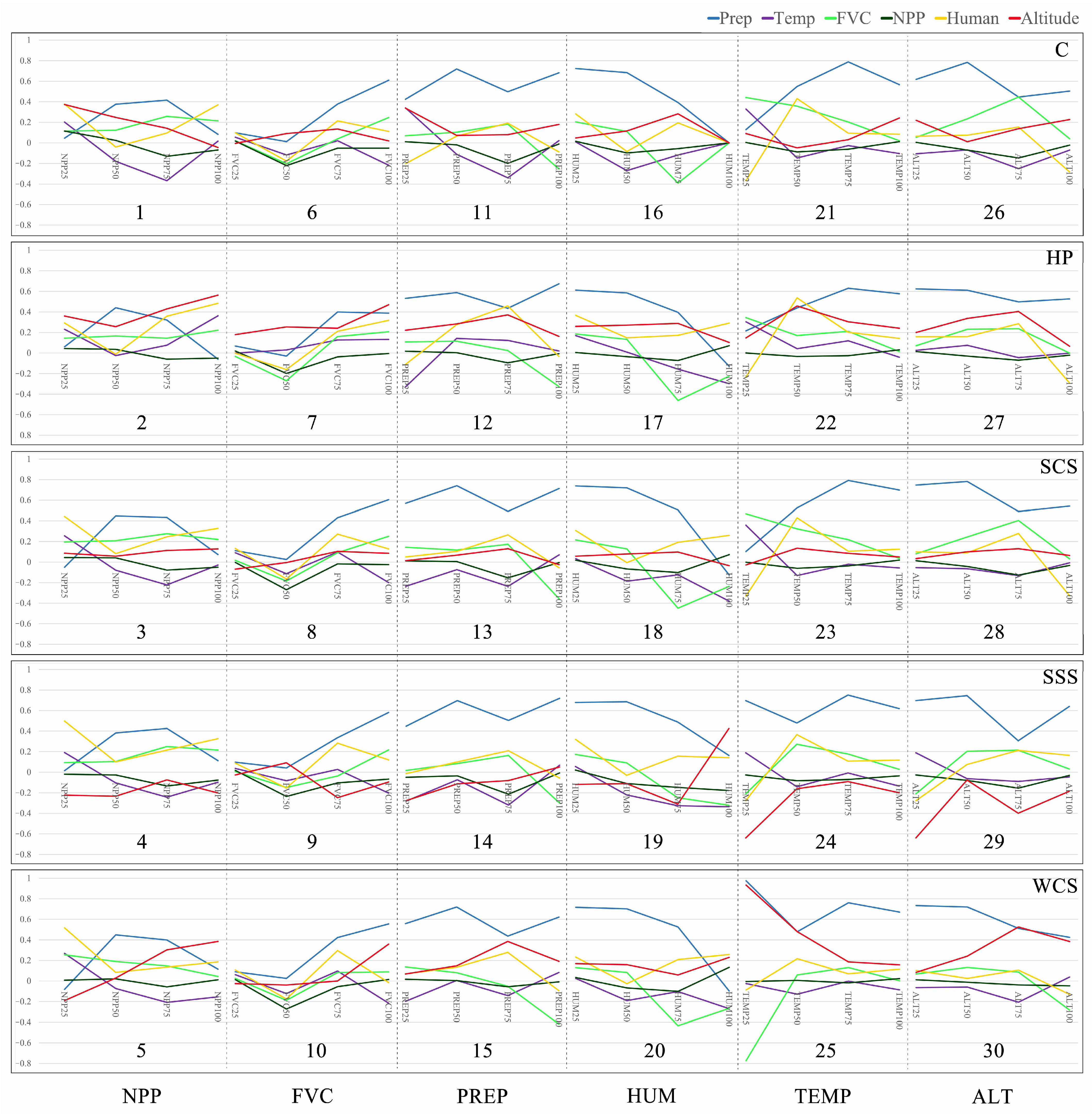
The effects of environmental gradients: This study highlights that single factors exhibit varying effects on ES at different environmental gradients, including anthropogenic gradients. High altitude and high fractional vegetation cover (FVC) were found to contribute significantly to WCS.

Understanding these relationships between ecosystems and influencing factors can aid ecosystem management. Managers can consider local conditions and control influential factors accordingly, or strategically enhance specific ecosystem services to maximize overall benefits and achieve sustainable development of ES. We recommend maximizing the dominant effect of precipitation and rationalizing the imposition of positive human activities, such as human-induced regeneration of forest cover, in areas where precipitation is abundant to link ecosystem services to human well-being as much as possible. Overall, this research provides valuable insights into the dynamics of ES in the LPES region, shedding light on the interplay between climate change, human activities, and ecosystem services. These findings can guide decision-making processes and facilitate effective management and planning of the LPES areas for sustainable development.

References

- Costanza, R.; d’Arge, R.; de Groot, R.; Farber, S.; Grasso, M.; Hannon, B.; Limburg, K.; Naeem, S.; Oneill, R.V.; Paruelo, J.; et al. The value of the world’s ecosystem services and natural capital. Nature 1997, 387, 253–260. [Google Scholar] [CrossRef]
- Berry, Z.C.; Jones, K.W.; Aguilar, L.R.G.; Congalton, R.G.; Holwerda, F.; Kolka, R.; Looker, N.; Ramirez, S.M.L.; Manson, R.; Mayer, A.; et al. Evaluating ecosystem service trade-offs along a land-use intensification gradient in central Veracruz, Mexico. Ecosyst. Serv. 2020, 45, 101181. [Google Scholar] [CrossRef]
- Belaire, J.A.; Higgins, C.; Zoll, D.; Lieberknecht, K.; Bixler, R.P.; Neff, J.L.; Keitt, T.H.; Jha, S. Fine-scale monitoring and mapping of biodiversity and ecosystem services reveals multiple synergies and few tradeoffs in urban green space management. Sci. Total Environ. 2022, 849, 157801. [Google Scholar] [CrossRef]
- Li, S.; Xie, A.; Lyu, C.; Guo, X. Research Progress and Prospect for Land Ecosystem Services. China Land Sci. 2018, 32, 82–89. [Google Scholar]
- Hasan, S.S.; Zhen, L.; Miah, M.G.; Ahamed, T.; Samie, A. Impact of land use change on ecosystem services: A review. Environ. Dev. 2020, 34, 100527. [Google Scholar] [CrossRef]
- Fu, B.; Zhang, L. Land-use change and ecosystem services: Concepts, methods and progress. Prog. Geogr. 2014, 33, 441–446. [Google Scholar]
- Huang, C.; Yang, J.; Zhang, W. Development of ecosystem services evaluation models: Research progress. Chin. J. Ecol. 2013, 32, 3360–3367. [Google Scholar]
- Bagstad, K.J.; Johnson, G.W.; Voigt, B.; Villa, F. Spatial dynamics of ecosystem service flows: A comprehensive approach to quantifying actual services. Ecosyst. Serv. 2013, 4, 117–125. [Google Scholar] [CrossRef]
- Mace, G.M.; Norris, K.; Fitter, A.H. Biodiversity and ecosystem services: A multilayered relationship. Trends Ecol. Evol. 2012, 27, 19–26. [Google Scholar] [CrossRef]
- Haase, D.; Schwarz, N.; Strohbach, M.; Kroll, F.; Seppelt, R. Synergies, Trade-offs, and Losses of Ecosystem Services in Urban Regions: An Integrated Multiscale Framework Applied to the Leipzig-Halle Region, Germany. Ecol. Soc. 2012, 17, 1–22. [Google Scholar] [CrossRef]
- Wei, C.W.; Su, K.; Jiang, X.B.; You, Y.F.; Zhou, X.B.; Yu, Z.; Chen, Z.C.; Liao, Z.H.; Zhang, Y.M.; Wang, L.Y. Increase in precipitation and fractional vegetation cover promote synergy of ecosystem services in China’s arid regions-Northern sand-stabilization belt. Front. Ecol. Evol. 2023, 11, 1116484. [Google Scholar] [CrossRef]
- Su, K.; Liu, H.J.; Wang, H.Y. Spatial-Temporal Changes and Driving Force Analysis of Ecosystems in the Loess Plateau Ecological Screen. Forests 2022, 13, 54. [Google Scholar] [CrossRef]
- Wood, E.M.; Pidgeon, A.M. Extreme variations in spring temperature affect ecosystem regulating services provided by birds during migration. Ecosphere 2015, 6, 1–16. [Google Scholar] [CrossRef]
- Li, P.; Omani, N.; Chaubey, I.; Wei, X.M. Evaluation of Drought Implications on Ecosystem Services: Freshwater Provisioning and Food Provisioning in the Upper Mississippi River Basin. Int. J. Environ. Res. Public Health 2017, 14, 496. [Google Scholar] [CrossRef] [PubMed]
- Canelas, J.V.; Pereira, H.M. Impacts of land-use intensity on ecosystems stability. Ecol. Model. 2022, 472, 110093. [Google Scholar] [CrossRef]
- Balvanera, P.; Pfisterer, A.B.; Buchmann, N.; He, J.S.; Nakashizuka, T.; Raffaelli, D.; Schmid, B. Quantifying the evidence for biodiversity effects on ecosystem functioning and services. Ecol. Lett. 2006, 9, 1146–1156. [Google Scholar] [CrossRef] [PubMed]
- Allan, E.; Manning, P.; Alt, F.; Binkenstein, J.; Blaser, S.; Bluethgen, N.; Bohm, S.; Grassein, F.; Holzel, N.; Klaus, V.H.; et al. Land use intensification alters ecosystem multifunctionality via loss of biodiversity and changes to functional composition. Ecol. Lett. 2015, 18, 834–843. [Google Scholar] [CrossRef]
- Smale, D.A. Impacts of ocean warming on kelp forest ecosystems. New Phytol. 2020, 225, 1447–1454. [Google Scholar] [CrossRef]
- Nelson, G.C.; Bennett, E.; Berhe, A.A.; Cassman, K.; DeFries, R.; Dietz, T.; Dobermann, A.; Dobson, A.; Janetos, A.; Levy, M.; et al. Anthropogenic drivers of ecosystem change: An overview. Ecol. Soc. 2006, 11, 1–31. [Google Scholar] [CrossRef]
- Mayer, A.; Kaufmann, L.; Kalt, G.; Matej, S.; Theurl, M.C.; Morais, T.G.; Leip, A.; Erb, K.H. Applying the Human Appropriation of Net Primary Production framework to map provisioning ecosystem services and their relation to ecosystem functioning across the European Union. Ecosyst. Serv. 2021, 51, 101344. [Google Scholar] [CrossRef]
- Kumar, M.; Savita; Singh, H.; Pandey, R.; Singh, M.P.; Ravindranath, N.H.; Kalra, N. Assessing vulnerability of forest ecosystem in the Indian Western Himalayan region using trends of net primary productivity. Biodivers. Conserv. 2019, 28, 2163–2182. [Google Scholar] [CrossRef]
- Briner, S.; Huber, R.; Bebi, P.; Elkin, C.; Schmatz, D.R.; Gret-Regamey, A. Trade-Offs between Ecosystem Services in a Mountain Region. Ecol. Soc. 2013, 18, 35. [Google Scholar] [CrossRef]
- Aparecido, L.M.T.; Teodoro, G.S.; Mosquera, G.; Brum, M.; Barros, F.D.; Pompeu, P.V.; Rodas, M.; Lazo, P.; Muller, C.S.; Mulligan, M.; et al. Ecohydrological drivers of Neotropical vegetation in montane ecosystems. Ecohydrology 2018, 11, e1932. [Google Scholar] [CrossRef]
- Garcia-Llamas, P.; Geijzendorffer, I.R.; Garcia-Nieto, A.P.; Calvo, L.; Suarez-Seoane, S.; Cramer, W. Impact of land cover change on ecosystem service supply in mountain systems: A case study in the Cantabrian Mountains (NW of Spain). Reg. Environ. Chang. 2019, 19, 529–542. [Google Scholar] [CrossRef]
- Mahdavi, P.; Akhani, H.; Van der Maarel, E. Species Diversity and Life-Form Patterns in Steppe Vegetation along a 3000 m Altitudinal Gradient in the Alborz Mountains, Iran. Folia Geobot. 2013, 48, 7–22. [Google Scholar] [CrossRef]
- Yu, Y.Y.; Li, J.; Zhou, Z.X.; Ma, X.P.; Zhang, X.F. Response of multiple mountain ecosystem services on environmental gradients: How to respond, and where should be priority conservation? J. Clean. Prod. 2021, 278, 123264. [Google Scholar] [CrossRef]
- Liu, L.B.; Wang, Z.; Wang, Y.; Zhang, Y.T.; Shen, J.S.; Qin, D.H.; Li, S.C. Trade-off analyses of multiple mountain ecosystem services along elevation, vegetation cover and precipitation gradients: A case study in the Taihang Mountains. Ecol. Indic. 2019, 103, 94–104. [Google Scholar] [CrossRef]
- Becker, A.; Korner, C.; Brun, J.J.; Guisan, A.; Tappeiner, U. Ecological and land use studies along elevational gradients. Mt. Res. Dev. 2007, 27, 58–65. [Google Scholar] [CrossRef]
- Ma, S.; Qiao, Y.P.; Wang, L.J.; Zhang, J.C. Terrain gradient variations in ecosystem services of different vegetation types in mountainous regions: Vegetation resource conservation and sustainable development. For. Ecol. Manag. 2021, 482, 118856. [Google Scholar] [CrossRef]
- Gomes, L.C.; Bianchi, F.; Cardoso, I.M.; Fernandes, E.I.; Schulte, R.P.O. Land use change drives the spatio-temporal variation of ecosystem services and their interactions along an altitudinal gradient in Brazil. Landsc. Ecol. 2020, 35, 1571–1586. [Google Scholar] [CrossRef]
- Sundqvist, M.K.; Sanders, N.J.; Wardle, D.A. Community and Ecosystem Responses to Elevational Gradients: Processes, Mechanisms, and Insights for Global Change. Annu. Rev. Ecol. Evol. Syst. 2013, 44, 261–280. [Google Scholar] [CrossRef]
- Wu, J.H.; Wang, G.Z.; Chen, W.X.; Pan, S.P.; Zeng, J. Terrain gradient variations in the ecosystem services value of the Qinghai-Tibet Plateau, China. Glob. Ecol. Conserv. 2022, 34, e02008. [Google Scholar] [CrossRef]
- Canedoli, C.; Ferre, C.; Abu El Khair, D.; Comolli, R.; Liga, C.; Mazzucchelli, F.; Proietto, A.; Rota, N.; Colombo, G.; Bassano, B.; et al. Evaluation of ecosystem services in a protected mountain area: Soil organic carbon stock and biodiversity in alpine forests and grasslands. Ecosyst. Serv. 2020, 44, 101135. [Google Scholar] [CrossRef]
- Garca-Llorente, M.; Iniesta-Arandia, I.; Willaarts, B.A.; Harrison, P.A.; Berry, P.; Bayo, M.D.; Castro, A.J.; Montes, C.; Martin-Lopez, B. Biophysical and sociocultural factors underlying spatial trade-offs of ecosystem services in semiarid watersheds. Ecol. Soc. 2015, 20, 39. [Google Scholar] [CrossRef]
- Juerges, N.; Arts, B.; Masiero, M.; Hoogstra-Klein, M.; Borges, J.G.; Brodrechtova, Y.; Brukas, V.; Canadas, M.J.; Carvalho, P.O.; Corradini, G.; et al. Power analysis as a tool to analyse trade-offs between ecosystem services in forest management: A case study from nine European countries. Ecosyst. Serv. 2021, 49, 101290. [Google Scholar] [CrossRef]
- Pena, L.; Onaindia, M.; de Manuel, B.F.; Ametzaga-Arregi, I.; Casado-Arzuaga, I. Analysing the Synergies and Trade-Offs between Ecosystem Services to Reorient Land Use Planning in Metropolitan Bilbao (Northern Spain). Sustainability 2018, 10, 4376. [Google Scholar] [CrossRef]
- Wam, H.K.; Bunnefeld, N.; Clarke, N.; Hofstad, O. Conflicting interests of ecosystem services: Multi-criteria modelling and indirect evaluation of trade-offs between monetary and non-monetary measures. Ecosyst. Serv. 2016, 22, 280–288. [Google Scholar] [CrossRef]
- Lavorel, S.; Grigulis, K. How fundamental plant functional trait relationships scale-up to trade-offs and synergies in ecosystem services. J. Ecol. 2012, 100, 128–140. [Google Scholar] [CrossRef]
- Le Provost, G.; Schenk, N.V.; Penone, C.; Thiele, J.; Westphal, C.; Allan, E.; Ayasse, M.; Bluthgen, N.; Boeddinghaus, R.S.; Boesing, A.L.; et al. The supply of multiple ecosystem services requires biodiversity across spatial scales. Nat. Ecol. Evol. 2023, 7, 236–249. [Google Scholar] [CrossRef]
- Liang, W.; Fu, B.J.; Wang, S.; Zhang, W.B.; Jin, Z.; Feng, X.M.; Yan, J.W.; Liu, Y.; Zhou, S. Quantification of the ecosystem carrying capacity on China’s Loess Plateau. Ecol. Indic. 2019, 101, 192–202. [Google Scholar] [CrossRef]
- Hu, Y.; Ma, L.; Li, R.; Ke, Z.; Yang, J.; Liu, Z. Factor analysis of underground biomass in forest ecosystem on the Loess Plateau. Acta Ecol. Sin. 2021, 41, 8643–8653. [Google Scholar]
- Zhao, X.; Ma, P.; Li, W.; Du, Y. Spatiotemporal changes of supply and demand relationships of ecosystem services in the Loess Plateau. Acta Geogr. Sin. 2021, 76, 2780–2796. [Google Scholar]
- Wang, S.; Fu, B.; Wu, X.; Wang, Y. Dynamics and sustainability of social-ecological systems in the Loess Plateau. Resour. Sci. 2020, 42, 96–103. [Google Scholar] [CrossRef]
- Zhang, Y.M.; Su, K.; Jiang, X.B.; You, Y.F.; Zhou, X.B.; Yu, Z.; Chen, Z.C.; Wang, L.Y.; Wei, C.W.; Liao, Z.H. Response of ecosystem services to impervious surface changes and their scaling effects in Loess Plateau ecological Screen, China. Ecol. Indic. 2023, 147, 109997. [Google Scholar] [CrossRef]
- Xu, K.J.; Tian, Q.J.; Yang, Y.J.; Yue, J.B.; Tang, S.F. How up-scaling of remote-sensing images affects land-cover classification by comparison with multiscale satellite images. Int. J. Remote Sens. 2019, 40, 2784–2810. [Google Scholar] [CrossRef]
- Wu, S.; Li, J.; Huang, G.H. A study on DEM-derived primary topographic attributes for hydrologic applications: Sensitivity to elevation data resolution. Appl. Geogr. 2008, 28, 210–223. [Google Scholar] [CrossRef]
- Zhang, H.Y.; Fan, J.W.; Cao, W.; Harris, W.; Li, Y.Z.; Chi, W.F.; Wang, S.Z. Response of wind erosion dynamics to climate change and human activity in Inner Mongolia, China during 1990 to 2015. Sci. Total Environ. 2018, 639, 1038–1050. [Google Scholar] [CrossRef] [PubMed]
- Xu, W.X.; Wang, J.M.; Zhang, M.; Li, S.J. Construction of landscape ecological network based on landscape ecological risk assessment in a large-scale opencast coal mine area. J. Clean. Prod. 2021, 286, 125523. [Google Scholar] [CrossRef]
- Pi, X.; Zeng, Y.; He, C. High-resolution urban vegetation coverage estimation based on multi-source remote sensing data fusion. J. Remote Sens. 2021, 25, 1216–1226. [Google Scholar] [CrossRef]
- Ma, Y.F.; Liu, S.M.; Song, L.S.; Xu, Z.W.; Liu, Y.L.; Xu, T.R.; Zhu, Z.L. Estimation of daily evapotranspiration and irrigation water efficiency at a Landsat-like scale for an arid irrigation area using multi-source remote sensing data. Remote Sens. Environ. 2018, 216, 715–734. [Google Scholar] [CrossRef]
- Luo, X.; Yang, J.; Sun, W.; He, B.J. Suitability of human settlements in mountainous areas from the perspective of ventilation: A case study of the main urban area of Chongqing. J. Clean. Prod. 2021, 310, 127467. [Google Scholar] [CrossRef]
- Fryrear, D.W.; Bilbro, J.D.; Saleh, A.; Schomberg, H.; Stout, J.E.; Zobeck, T.M. RWEQ: Improved wind erosion technology. J. Soil Water Conserv. 2000, 55, 183–189. [Google Scholar] [CrossRef]
- Guo, B.; Zhang, F.F.; Yang, G.; Sun, C.H.; Han, F.; Jiang, L. Improved estimation method of soil wind erosion based on remote sensing and geographic information system in the Xinjiang Uygur Autonomous Region, China. Geomat. Nat. Hazards Risk 2017, 8, 1752–1767. [Google Scholar] [CrossRef]
- Su, K.; Sun, X.T.; Guo, H.Q.; Long, Q.Q.; Li, S.; Mao, X.Q.; Niu, T.; Yu, Q.; Wang, Y.R.; Yue, D.P. The establishment of a cross-regional differentiated ecological compensation scheme based on the benefit areas and benefit levels of sand-stabilization ecosystem service. J. Clean. Prod. 2020, 270, 122490. [Google Scholar] [CrossRef]
- Gong, G.; Liu, J.; Shao, Q. Wind erosion in Xilingol League, Inner Mongolia since the 1990s using the Revised Wind Erosion Equation. Prog. Geogr. 2014, 33, 825–834. [Google Scholar]
- Thomsen, L.M.; Baartman, J.E.M.; Barneveld, R.J.; Starkloff, T.; Stolte, J. Soil surface roughness: Comparing old and new measuring methods and application in a soil erosion model. Soil 2015, 1, 399–410. [Google Scholar] [CrossRef]
- Saleh, A.; Fryear, D.W.; Bilbro, J.D. Aerodynamic roughness prediction from soil surface roughness measurement. Soil Sci. 1997, 162, 205–210. [Google Scholar] [CrossRef]
- Kong, L.Q.; Zheng, H.; Rao, E.M.; Xiao, Y.; Ouyang, Z.Y.; Li, C. Evaluating indirect and direct effects of eco-restoration policy on soil conservation service in Yangtze River Basin. Sci. Total Environ. 2018, 631–632, 887–894. [Google Scholar] [CrossRef]
- Pandey, A.; Chowdary, V.M.; Mal, B.C. Identification of critical erosion prone areas in the small agricultural watershed using USLE, GIS and remote sensing. Water Resour. Manag. 2007, 21, 729–746. [Google Scholar] [CrossRef]
- Zhang, W.; Xie, Y.; Liu, B. Rainfall Erosivity Estimation Using Daily Rainfall Amounts. Sci. Geogr. Sin. 2002, 22, 705–711. [Google Scholar]
- Bhuyan, S.J.; Kalita, P.K.; Janssen, K.A.; Barnes, P.L. Soil loss predictions with three erosion simulation models. Environ. Model. Softw. 2002, 17, 137–146. [Google Scholar] [CrossRef]
- Nearing, M.A. A single, continuous function for slope steepness influence on soil loss. Soil Sci. Soc. Am. J. 1997, 61, 917–919. [Google Scholar] [CrossRef]
- Fistikoglu, O.; Harmancioglu, N.B. Integration of GIS with USLE in assessment of soil erosion. Water Resour. Manag. 2002, 16, 447–467. [Google Scholar] [CrossRef]
- Zhang, L.; Dawes, W.R.; Walker, G.R. Response of mean annual evapotranspiration to vegetation changes at catchment scale. Water Resour. Res. 2001, 37, 701–708. [Google Scholar] [CrossRef]
- Piao, S.L.; Fang, J.Y.; Ciais, P.; Peylin, P.; Huang, Y.; Sitch, S.; Wang, T. The carbon balance of terrestrial ecosystems in China. Nature 2009, 458, 1009–1013. [Google Scholar] [CrossRef] [PubMed]
- Fang, J.Y.; Chen, A.P.; Peng, C.H.; Zhao, S.Q.; Ci, L. Changes in forest biomass carbon storage in China between 1949 and 1998. Science 2001, 292, 2320–2322. [Google Scholar] [CrossRef] [PubMed]
- Bryan, B.A.; Nolan, M.; Harwood, T.D.; Connor, J.D.; Navarro-Garcia, J.; King, D.; Summers, D.M.; Newth, D.; Cai, Y.; Grigg, N.; et al. Supply of carbon sequestration and biodiversity services from Australia’s agricultural land under global change. Glob. Environ. Chang. Hum. Policy Dimens. 2014, 28, 166–181. [Google Scholar] [CrossRef]
- Huang, L.; Liu, J.; Shao, Q.; Deng, X. Temporal and spatial patterns of carbon sequestration services for primary terrestrial ecosystems in China between 1990 and 2030. Acta Ecol. Sin. 2016, 36, 3891–3902. [Google Scholar]
- Liu, W.; Yan, Y.; Wang, D.; Ma, W. Integrate carbon dynamics models for assessing the impact of land use intervention on carbon sequestration ecosystem service. Ecol. Indic. 2018, 91, 268–277. [Google Scholar] [CrossRef]
- Ruijs, A.; Wossink, A.; Kortelainen, M.; Alkemade, R.; Schulp, C.J.E. Trade-off analysis of ecosystem services in Eastern Europe. Ecosyst. Serv. 2013, 4, 82–94. [Google Scholar] [CrossRef]
- Zhai, T.; Wang, J.; Fang, Y.; Huang, L.; Liu, J.; Zhao, C. Integrating Ecosystem Services Supply, Demand and Flow in Ecological Compensation: A Case Study of Carbon Sequestration Services. Sustainability 2021, 13, 1668. [Google Scholar] [CrossRef]
- Wu, L.L.; Sun, C.G.; Fan, F.L. Estimating the Characteristic Spatiotemporal Variation in Habitat Quality Using the InVEST Model-A Case Study from Guangdong-Hong Kong-Macao Greater Bay Area. Remote Sens. 2021, 13, 1008. [Google Scholar] [CrossRef]
- Aneseyee, A.B.; Noszczyk, T.; Soromessa, T.; Elias, E. The InVEST Habitat Quality Model Associated with Land Use/Cover Changes: A Qualitative Case Study of the Winike Watershed in the Omo-Gibe Basin, Southwest Ethiopia. Remote Sens. 2020, 12, 1103. [Google Scholar] [CrossRef]
- Alamgir, M.; Turton, S.M.; Macgregor, C.J.; Pert, P.L. Ecosystem services capacity across heterogeneous forest types: Understanding the interactions and suggesting pathways for sustaining multiple ecosystem services. Sci. Total Environ. 2016, 566, 584–595. [Google Scholar] [CrossRef] [PubMed]
- Brockerhoff, E.G.; Barbaro, L.; Castagneyrol, B.; Forrester, D.I.; Gardiner, B.; Gonzalez-Olabarria, J.R.; Lyver, P.O.; Meurisse, N.; Oxbrough, A.; Taki, H.; et al. Forest biodiversity, ecosystem functioning and the provision of ecosystem services. Biodivers. Conserv. 2017, 26, 3005–3035. [Google Scholar] [CrossRef]
- Dobson, A.; Lodge, D.; Alder, J.; Cumming, G.S.; Keymer, J.; McGlade, J.; Mooney, H.; Rusak, J.A.; Sala, O.; Wolters, V.; et al. Habitat loss, trophic collapse, and the decline of ecosystem services. Ecology 2006, 87, 1915–1924. [Google Scholar] [CrossRef] [PubMed]
- Nelson, E.; Sander, H.; Hawthorne, P.; Conte, M.; Ennaanay, D.; Wolny, S.; Manson, S.; Polasky, S. Projecting Global Land-Use Change and Its Effect on Ecosystem Service Provision and Biodiversity with Simple Models. PLoS ONE 2010, 5, e14327. [Google Scholar] [CrossRef]
- Ouyang, Z.; Zheng, H.; Xiao, Y.; Polasky, S.; Liu, J.; Xu, W.; Wang, Q.; Zhang, L.; Xiao, Y.; Rao, E.; et al. Improvements in ecosystem services from investments in natural capital. Science 2016, 352, 1455–1459. [Google Scholar] [CrossRef]
- Terrado, M.; Sabater, S.; Chaplin-Kramer, B.; Mandle, L.; Ziv, G.; Acuna, V. Model development for the assessment of terrestrial and aquatic habitat quality in conservation planning. Sci. Total Environ. 2016, 540, 63–70. [Google Scholar] [CrossRef]
- Bhagabati, N.K.; Ricketts, T.; Sulistyawan, T.B.S.; Conte, M.; Ennaanay, D.; Hadian, O.; McKenzie, E.; Olwero, N.; Rosenthal, A.; Tallis, H.; et al. Ecosystem services reinforce Sumatran tiger conservation in land use plans. Biol. Conserv. 2014, 169, 147–156. [Google Scholar] [CrossRef]
- Bennett, E.M.; Peterson, G.D.; Gordon, L.J. Understanding relationships among multiple ecosystem services. Ecol. Lett. 2009, 12, 1394–1404. [Google Scholar] [CrossRef] [PubMed]
- Rodriguez, J.P.; Beard, T.D.; Bennett, E.M.; Cumming, G.S.; Cork, S.J.; Agard, J.; Dobson, A.P.; Peterson, G.D. Trade-offs across space, time, and ecosystem services. Ecol. Soc. 2006, 11, 1–14. [Google Scholar] [CrossRef]
- Turner, K.G.; Odgaard, M.V.; Bocher, P.K.; Dalgaard, T.; Svenning, J.-C. Bundling ecosystem services in Denmark: Trade-offs and synergies in a cultural landscape. Landsc. Urban Plan. 2014, 125, 89–104. [Google Scholar] [CrossRef]
- Spake, R.; Lasseur, R.; Crouzat, E.; Bullock, J.M.; Lavorel, S.; Parks, K.E.; Schaafsma, M.; Bennett, E.M.; Maes, J.; Mulligan, M.; et al. Unpacking ecosystem service bundles: Towards predictive mapping of synergies and trade-offs between ecosystem services. Glob. Environ. Chang. Hum. Policy Dimens. 2017, 47, 37–50. [Google Scholar] [CrossRef]
- Howe, C.; Suich, H.; Vira, B.; Mace, G.M. Creating win-wins from trade-offs? Ecosystem services for human well-being: A meta-analysis of ecosystem service trade-offs and synergies in the real world. Glob. Environ. Chang. Hum. Policy Dimens. 2014, 28, 263–275. [Google Scholar] [CrossRef]
- Schober, P.; Boer, C.; Schwarte, L.A. Correlation Coefficients: Appropriate Use and Interpretation. Anesth. Analg. 2018, 126, 1763–1768. [Google Scholar] [CrossRef] [PubMed]
- Smith, P.; House, J.I.; Bustamante, M.; Sobocka, J.; Harper, R.; Pan, G.; West, P.C.; Clark, J.M.; Adhya, T.; Rumpel, C.; et al. Global change pressures on soils from land use and management. Glob. Chang. Biol. 2016, 22, 1008–1028. [Google Scholar] [CrossRef]
- Isbell, F.; Gonzalez, A.; Loreau, M.; Cowles, J.; Diaz, S.; Hector, A.; Mace, G.M.; Wardle, D.A.; O’Connor, M.I.; Duffy, J.E.; et al. Linking the influence and dependence of people on biodiversity across scales. Nature 2017, 546, 65–72. [Google Scholar] [CrossRef]
- Chagnon, M.; Kreutzweiser, D.; Mitchell, E.A.; Mitchell, E.A.; Morrissey, C.A.; Noome, D.A.; Noome, D.A.; Van der Sluijs, J.P.; Van der Sluijs, J.P. Risks of large-scale use of systemic insecticides to ecosystem functioning and services. Environ. Sci. Pollut. Res. 2015, 22, 119–134. [Google Scholar] [CrossRef]
- Fischer, A.; Eastwood, A. Coproduction of ecosystem services as human-nature interactions-An analytical framework. Land Use Policy 2016, 52, 41–50. [Google Scholar] [CrossRef]
- Fang, L.; Wang, L.; Chen, W.; Sun, J.; Cao, Q.; Wang, S.; Wang, L. Identifying the impacts of natural and human factors on ecosystem service in the Yangtze and Yellow River Basins. J. Clean. Prod. 2021, 314, 127995. [Google Scholar] [CrossRef]
- Burkhard, B.; Kroll, F.; Nedkov, S.; Mueller, F. Mapping ecosystem service supply, demand and budgets. Ecol. Indic. 2012, 21, 17–29. [Google Scholar] [CrossRef]
- Yang, B.; Wang, Z.; Zhang, H.; Tan, L. Spatial pattern evolution characteristics and driving mechanism of rural settlements in high mountain areas with poverty. Trans. Chin. Soc. Agric. Eng. 2021, 37, 285–293. [Google Scholar]
- Seto, K.C.; Fragkias, M.; Guneralp, B.; Reilly, M.K. A Meta-Analysis of Global Urban Land Expansion. PLoS ONE 2011, 6, e23777. [Google Scholar] [CrossRef]
- Carr, D. Population and deforestation: Why rural migration matters. Prog. Hum. Geogr. 2009, 33, 355–378. [Google Scholar] [CrossRef]
- Zheng, F.; Tang, K.; Bai, H. Study on Relationship between Human’s Activities and Environmental evolution. Res. Soil Water Conserv. 1994, 1, 36–42. [Google Scholar]
- Yang, Z.; Dong, J.; Xu, X.; Zhao, G.; Chen, W.; Zhou, Y. Spatiotemporal pattern of forest fragmentation in the Loess Plateau. Resour. Sci. 2018, 40, 1246–1255. [Google Scholar] [CrossRef]
- Wang, F.; Li, R.; Xie, Y. Analysis on Eco-environment Construction in Human Period on Loess Plateau. Res. Soil Water Conserv. 2001, 8, 138–142. [Google Scholar]
- Li, Q. Characteristics and development of grassland ecological environment on the northwestern loess plateau. Pratacultural Sci. 1998, 15, 1–8. [Google Scholar]
- Dijkstra, T.K.; Henseler, J. Consistent and asymptotically normal PLS estimators for linear structural equations. Comput. Stat. Data Anal. 2015, 81, 10–23. [Google Scholar] [CrossRef]
- You, Y.F.; Wang, S.Y.; Pan, N.Q.; Ma, Y.X.; Liu, W.H. Growth stage-dependent responses of carbon fixation process of alpine grasslands to climate change over the Tibetan Plateau, China. Agric. For. Meteorol. 2020, 291, 108085. [Google Scholar] [CrossRef]
- Gao, Y.H.; Zhou, X.; Wang, Q.; Wang, C.Z.; Zhan, Z.M.; Chen, L.F.; Yan, J.X.; Qu, R. Vegetation net primary productivity and its response to climate change during 2001–2008 in the Tibetan Plateau. Sci. Total Environ. 2013, 444, 356–362. [Google Scholar] [CrossRef] [PubMed]
- Li, Z.; Liu, Z.; Chen, Z.; Yang, Z. The effects of climate changes on the productivity in the Inner Mongolia steppe of China. Acta Prataculturae Sin. 2003, 12, 4–10. [Google Scholar]
- Mao, D.H.; Luo, L.; Wang, Z.M.; Zhang, C.H.; Ren, C.Y. Variations in net primary productivity and its relationships with warming climate in the permafrost zone of the Tibetan Plateau. J. Geogr. Sci. 2015, 25, 967–977. [Google Scholar] [CrossRef]
- Xu, M.H.; Zhao, Z.T.; Zhou, H.K.; Ma, L.; Liu, X.J. Plant Allometric Growth Enhanced by the Change in Soil Stoichiometric Characteristics with Depth in an Alpine Meadow Under Climate Warming. Front. Plant Sci. 2022, 13, 860980. [Google Scholar] [CrossRef] [PubMed]
- Zhu, X.; He, H.S.; Zhang, S.X.; Dijak, W.D.; Fu, Y.Y. Interactive Effects of Climatic Factors on Seasonal Vegetation Dynamics in the Central Loess Plateau, China. Forests 2019, 10, 1071. [Google Scholar] [CrossRef]
- Moura, M.R.; Villalobos, F.; Costa, G.C.; Garcia, P.C.A. Disentangling the Role of Climate, Topography and Vegetation in Species Richness Gradients. PLoS ONE 2016, 11, e152468. [Google Scholar] [CrossRef]
- Zhou, S.J.; Dong, Y.Q.; Julihaiti, A.; Nie, T.T.; Jiang, A.J.; An, S.Z. Spatial Variation in Desert Spring Vegetation Biomass, Richness and Their Environmental Controls in the Arid Region of Central Asia. Sustainability 2022, 14, 12152. [Google Scholar] [CrossRef]
- Zhang, H.Y.; Fan, J.W.; Cao, W.; Zhong, H.P.; Harris, W.; Gong, G.L.; Zhang, Y.X. Changes in multiple ecosystem services between 2000 and 2013 and their driving factors in the Grazing Withdrawal Program, China. Ecol. Eng. 2018, 116, 67–79. [Google Scholar] [CrossRef]
- Jia, X.X.; Shao, M.A.; Zhu, Y.J.; Luo, Y. Soil moisture decline due to afforestation across the Loess Plateau, China. J. Hydrol. 2017, 546, 113–122. [Google Scholar] [CrossRef]
- Feng, X.M.; Li, J.X.; Cheng, W.; Fu, B.J.; Wang, Y.Q.; Lu, Y.H.; Shao, M.A. Evaluation of AMSR-E retrieval by detecting soil moisture decrease following massive dryland re-vegetation in the Loess Plateau, China. Remote Sens. Environ. 2017, 196, 253–264. [Google Scholar] [CrossRef]
- Jing, P.Q.; Zhang, D.H.; Ai, Z.M.; Wu, H.J.; Zhang, D.M.; Ren, H.H.; Suo, L. Responses of Ecosystem Services to Climate Change: A Case Study of the Loess Plateau. Forests 2022, 13, 2011. [Google Scholar] [CrossRef]
- Zhang, H.D.; Wei, W.; Chen, L.D.; Yang, L. Evaluating canopy transpiration and water use of two typical planted tree species in the dryland Loess Plateau of China. Ecohydrology 2017, 10, e1830. [Google Scholar] [CrossRef]
- Urban, M.C. Accelerating extinction risk from climate change. Science 2015, 348, 571–573. [Google Scholar] [CrossRef] [PubMed]
- Bai, L.; Tian, J.L.; Peng, Y.; Huang, Y.H.; He, X.; Bai, X.Y.; Bai, T. Effects of climate change on ecosystem services and their components in southern hills and northern grasslands in China. Environ. Sci. Pollut. Res. 2021, 28, 44916–44935. [Google Scholar] [CrossRef] [PubMed]
- Lu, N.; Fu, B.J.; Jin, T.T.; Chang, R.Y. Trade-off analyses of multiple ecosystem services by plantations along a precipitation gradient across Loess Plateau landscapes. Landsc. Ecol. 2014, 29, 1697–1708. [Google Scholar] [CrossRef]
- Han, Q.J.; Qu, J.J.; Dong, Z.B.; Zhang, K.C.; Zu, R.P. Air density effects on aeolian sand movement: Implications for sediment transport and sand control in regions with extreme altitudes or temperatures. Sedimentology 2015, 62, 1024–1038. [Google Scholar] [CrossRef]
- Rosseel, Y. lavaan: An R Package for Structural Equation Modeling. J. Stat. Softw. 2012, 48, 1–36. [Google Scholar] [CrossRef]
- Langellotto, G.A.; Denno, R.F. Responses of invertebrate natural enemies to complex-structured habitats: A meta-analytical synthesis. Oecologia 2004, 139, 1–10. [Google Scholar] [CrossRef]
- Halaj, J.; Ross, D.W.; Moldenke, A.R. Importance of habitat structure to the arthropod food-web in Douglas-fir canopies. Oikos 2000, 90, 139–152. [Google Scholar] [CrossRef]
- Okin, G.S.; Gillette, D.A.; Herrick, J.E. Multi-scale controls on and consequences of aeolian processes in landscape change in arid and semi-arid environments. J. Arid Environ. 2006, 65, 253–275. [Google Scholar] [CrossRef]
- Wang, X.Z.; Wu, J.Z.; Liu, Y.L.; Hai, X.Y.; Shanguan, Z.P.; Deng, L. Driving factors of ecosystem services and their spatiotemporal change assessment based on land use types in the Loess Plateau. J. Environ. Manag. 2022, 311, 114835. [Google Scholar] [CrossRef] [PubMed]
- Jin, T.T.; Fu, B.J.; Liu, G.H.; Wang, Z. Hydrologic feasibility of artificial forestation in the semi-arid Loess Plateau of China. Hydrol. Earth Syst. Sci. 2011, 15, 2519–2530. [Google Scholar] [CrossRef]
- Piao, S.L.; Ciais, P.; Huang, Y.; Shen, Z.H.; Peng, S.S.; Li, J.S.; Zhou, L.P.; Liu, H.Y.; Ma, Y.C.; Ding, Y.H.; et al. The impacts of climate change on water resources and agriculture in China. Nature 2010, 467, 43–51. [Google Scholar] [CrossRef] [PubMed]
- Su, B.Q.; Su, Z.X.; Shangguan, Z.P. Trade-off analyses of plant biomass and soil moisture relations on the Loess Plateau. Catena 2021, 197, 104946. [Google Scholar] [CrossRef]
- Dodds, W.K.; Oakes, R.M. Headwater influences on downstream water quality. Environ. Manag. 2008, 41, 367–377. [Google Scholar] [CrossRef] [PubMed]
- Poudel, D.D.; Lee, T.; Srinivasan, R.; Abbaspour, K.; Jeong, C.Y. Assessment of seasonal and spatial variation of surface water quality, identification of factors associated with water quality variability, and the modeling of critical nonpoint source pollution areas in an agricultural watershed. J. Soil Water Conserv. 2013, 68, 155–171. [Google Scholar] [CrossRef]
- Li, M.; Shangguan, Z.; Deng, L. Spatial distribution of carbon storages in the terrestrial ecosystems and its influencing factors on the Loess Plateau. Acta Ecol. Sin. 2021, 41, 6786–6799. [Google Scholar]
- Warren, R.J. Mechanisms driving understory evergreen herb distributions across slope aspects: As derived from landscape position. Plant Ecol. 2008, 198, 297–308. [Google Scholar] [CrossRef]
- Wang, H.; Liu, G.H.; Li, Z.S.; Zhang, L.W.; Wang, Z.Z. Processes and driving forces for changing vegetation ecosystem services: Insights from the Shaanxi Province of China. Ecol. Indic. 2020, 112, 106105. [Google Scholar] [CrossRef]
- Cusack, D.F.; Karpman, J.; Ashdown, D.; Cao, Q.; Ciochina, M.; Halterman, S.; Lydon, S.; Neupane, A. Global change effects on humid tropical forests: Evidence for biogeochemical and biodiversity shifts at an ecosystem scale. Rev. Geophys. 2016, 54, 523–610. [Google Scholar] [CrossRef]
- Hou, W.; Gao, J.; Dai, E.; Peng, T.; Wu, S.; Wang, H. The runoff generation simulation and its spatial variation analysis in Sanchahe basin as the south source of Wujiang. Acta Geogr. Sin. 2018, 73, 1268–1282. [Google Scholar] [CrossRef]
- Ren, B.Y.; Wang, Q.F.; Zhang, R.R.; Zhou, X.Z.; Wu, X.P.; Zhang, Q. Assessment of Ecosystem Services: Spatio-Temporal Analysis and the Spatial Response of Influencing Factors in Hainan Province. Sustainability 2022, 14, 9145. [Google Scholar] [CrossRef]
- Dong, X.; Zhang, H.; Zhang, M. Explaining the diversity and endemic patterns based on phylogenetic approach for woody plants of the Loess Plateau. Biodivers. Sci. 2019, 27, 1269–1278. [Google Scholar]
- Xu, M.H.; Li, X.L.; Liu, M.; Shi, Y.; Zhou, H.K.; Zhang, B.G.; Yan, J.L. Spatial variation patterns of plant herbaceous community response to warming along latitudinal and altitudinal gradients in mountainous forests of the Loess Plateau, China. Environ. Exp. Bot. 2020, 172, 103983. [Google Scholar] [CrossRef]
- Zhang, C.Y.; Li, L.P.; Guan, Y.N.; Cai, D.L.; Chen, H.; Bian, X.L.; Guo, S. Impacts of vegetation properties and temperature characteristics on species richness patterns in drylands: Case study from Xinjiang. Ecol. Indic. 2021, 133, 108417. [Google Scholar] [CrossRef]
- Scott, R.L.; Jenerette, G.D.; Potts, D.L.; Huxman, T.E. Effects of seasonal drought on net carbon dioxide exchange from a woody-plant-encroached semiarid grassland. J. Geophys. Res. Biogeosciences 2009, 114, 900. [Google Scholar] [CrossRef]
- Keller, F.; Goyette, S.; Beniston, M. Sensitivity analysis of snow cover to climate change scenarios and their impact on plant habitats in alpine terrain. Clim. Chang. 2005, 72, 299–319. [Google Scholar] [CrossRef]
- Yang, H.J.; Gou, X.H.; Xue, B.; Ma, W.J.; Kuang, W.N.; Tu, Z.Y.; Gao, L.L.; Yin, D.C.; Zhang, J.Z. Research on the change of alpine ecosystem service value and its sustainable development path. Ecol. Indic. 2023, 146, 109893. [Google Scholar] [CrossRef]
- Zhang, J. Theory and Techniques of Vegetation Restoration and Construction on Loess Plateau, China. J. Soil Water Conserv. 2004, 18, 120–124. [Google Scholar] [CrossRef]
- Tang, X.L.; Zhao, X.; Bai, Y.F.; Tang, Z.Y.; Wang, W.T.; Zhao, Y.C.; Wan, H.W.; Xie, Z.Q.; Shi, X.Z.; Wu, B.F.; et al. Carbon pools in China’s terrestrial ecosystems: New estimates based on an intensive field survey. Proc. Natl. Acad. Sci. USA 2018, 115, 4021–4026. [Google Scholar] [CrossRef]
- Ma, S.; Wang, L.J.; Jiang, J.; Chu, L.; Zhang, J.C. Threshold effect of ecosystem services in response to climate change and vegetation coverage change in the Qinghai-Tibet Plateau ecological shelter. J. Clean. Prod. 2021, 318, 128592. [Google Scholar] [CrossRef]
- Behera, M.D.; Kushwaha, S.P.S. An analysis of altitudinal behavior of tree species in Subansiri district, Eastern Himalaya. Biodivers. Conserv. 2007, 16, 1851–1865. [Google Scholar] [CrossRef]