Article

A Spatial–Temporal Bayesian Deep Image Prior Model for Moderate Resolution Imaging Spectroradiometer Temporal Mixture Analysis

1
School of Land Science and Technology, China University of Geosciences, Beijing 100083, China
2
Aerospace Era Feihong Technology Co., Ltd., Beijing 100094, China
3
Department of Systems Design Engineering, University of Waterloo, Waterloo, ON N2L 3G1, Canada
*
Author to whom correspondence should be addressed.
These authors contributed equally to this work.
Remote Sens. 2023, 15(15), 3782; https://doi.org/10.3390/rs15153782
Submission received: 4 June 2023 / Revised: 24 July 2023 / Accepted: 27 July 2023 / Published: 29 July 2023
(This article belongs to the Special Issue Advances in Agricultural Remote Sensing and Artificial Intelligence)

Abstract

:
Time-series remote sensing images are important in agricultural monitoring and investigation. However, most time-series data with high temporal resolution have the problem of insufficient spatial resolution which cannot meet the requirement of precision agriculture. The unmixing technique can obtain the object abundances with richer spatial information from the coarse-resolution images. Although the unmixing technique is widely used in hyperspectral data, it is insufficiently researched for time-series data. Temporal unmixing extends spectral unmixing to the time domain from the spectral domain, and describes the temporal characteristics rather than the spectral characteristics of different ground objects. Deep learning (DL) techniques have achieved promising performance for the unmixing problem in recent years, but there are still few studies on temporal mixture analysis (TMA), especially in the application of crop phenological monitoring. This paper presents a novel spatial–temporal deep image prior method based on a Bayesian framework (ST-Bdip), which innovatively combines the knowledge-driven TMA model and the DL-driven model. The normalized difference vegetation index (NDVI) time series of moderate resolution imaging spectroradiometer (MODIS) data is used as the object for TMA, while the extracted seasonal crop signatures and the fractional coverages are perceived as the temporal endmembers (tEMs) and corresponding abundances. The proposed ST-Bdip method mainly includes the following contributions. First, a deep image prior model based on U-Net architecture is designed to efficiently learn the spatial context information, which enhances the representation of abundance modeling compared to the traditional non-negative least squares algorithm. Second, The TMA model is incorporated into the U-Net training process to exploit the knowledge in the forward temporal model effectively. Third, the temporal noise heterogeneity in time-series images is considered in the model optimization process. Specifically, the anisotropic covariance matrix of observations from different time dimensions is modeled as a multivariate Gaussian distribution and incorporated into the calculation of the loss function. Fourth, the "purified means" approach is used to further optimize crop tEMs and the corresponding abundances. Finally, the expectation–maximization (EM) algorithm is designed to solve the maximum a posterior (MAP) problem of the model in the Bayesian framework. Experimental results on three synthetic datasets with different noise levels and two real MODIS datasets demonstrate the superiority of the proposed approach in comparison with seven traditional and advanced unmixing algorithms.

1. Introduction

With the development of remote sensing technology, different Earth observation satellite sensors are widely used. Remote sensing data acquired in the same area show multi-platform, multi-sensor, multi-resolution, multi-spectral, and multi-temporal characteristics [1]. Time-series remote sensing images are significant for agricultural investigation [2], change detection applications [3], and environmental monitoring [4,5]. In general, high temporal remote sensing images usually cover a larger spatial range with a large image footprint but exhibit lower spatial resolution [1]. Therefore, mixed pixels in medium and low-resolution remote sensing data are an inevitable problem [6,7]. Each hybrid pixel is usually a combination of multiple land cover classes [8], while both the spectral reflectances and temporal growth curves of different classes are inconsistent. The spectral signal and temporal signal of a mixed pixel are composed of different “heterogeneous” components, while the spectral signal and temporal signal of a pure pixel represent only one class [9]. Compared with high-resolution remote sensing data, the coarse spatial resolution remote sensing data after the unmixing operation can provide more abundant temporal information and a wider coverage area. Therefore, searching for more effective unmixing methods to address the “mixed” problem in medium and low-resolution images remains a key concern.
Recently, traditional unmixing algorithms have usually been based on the linear spectral mixture model (LSMM) [10,11,12], which models the spectral reflectance of a single pixel as a linear combination of endmember reflectances, weighted by the abundance of each endmember within the pixel [6]. Liu et al. used LSMM for the unmixing of cotton, corn, tomato, and soil, and the experiments showed that LSMM achieves high efficiency, high precision, and strong adaptability [11]. The important process of unmixing can be divided into two tasks: endmember extraction and abundance estimation [13]. At present, most geometrical-based methods are commonly used for endmember extraction, including the vertex component analysis (VCA) [14], N-FINDR [15], and pixel purity index (PPI) [16]. Some researchers used cluster centers of Kmeans or KPmeans as endmembers, which employed the “Purified means” method, and also showed good performance by effective constraints on the derivation of endmembers [17,18]. However, it is difficult for these geometrical-based methods to extract accurate endmembers from highly mixed data because pure spectral features are not always available in reality [19]. In addition, fully constrained least squares (FCLS) [20] and sparse unmixing by variable splitting and augmented Lagrangian (SUnSAL) [21] algorithms are commonly used for abundance inversion [22], which usually need to assume that the pure endmember signatures exist in hyperspectral images. These algorithms are poorly inclusive of advanced modeling to solve the large-scale spatial correlation effects in remote sensing data. In recent years, deep learning (DL) methods have shown great capability and potential for spectral unmixing (SU) applications. Most of these DL-based methods are based on autoencoder (AE) networks [23,24,25] or convolutional neural networks (CNNs) [26,27,28]. Furthermore, the U-Net network, which uses fully convolutional layers, can better capture the large-scale spatial correlation effect of remote sensing data [29,30]. However, if there is ambiguous noise in images or the number of endmembers is incorrectly estimated, the unmixing performance usually drops drastically. Many DL-based methods consider the denoising algorithm as a module of the iterative optimization process in order to address the problem. For example, an untied denoising autoencoder with sparsity (uDAS) is proposed to formulate the unmixing problem, which improves the performance of abundance estimation [24]. And Zhao et al. propose a robust plug-and-play (PnP) priors framework for hyperspectral unmixing, which plugs a variety of denoisers to replace prior models and avoids designing regularizers [31]. However, the limited spectral information of the images and the restriction of sensor spatial resolution may directly lead to the low accuracy of ground object recognition and extraction [32]. And most of them are designed for the remote sensing data of a single day, mainly applied in SU application currently [27,33,34,35]. Few studies have focused on the temporal unmixing of continuous temporal remote sensing data.
Moderate Resolution Imaging Spectroradiometer (MODIS) data are widely used in large-scale monitoring of land cover types [36,37,38]. Many studies analyze phenological characteristics of remote sensing vegetation indices (VIs) of different crops in different seasons to realize the recognition of crop types [39,40,41,42]. However, the application of MODIS data is limited due to the low spatial resolution from multiple interferences, intimate mixtures, and resolution trade-offs. In recent years, the temporal mixture analysis (TMA) method [43] and TMA-based methods [44,45,46] are proposed to provide a new unmixing pattern for hypertemporal images (HTIs), which treat the temporal profiles of the mixed pixel as temporal endmembers (tEMs). TMA is an extension of spectral mixture analysis (SMA). And the algebraic expressions of TMA and SMA are identical in theory, except that TMA applies to the temporal spectra rather than the reflectance spectra. Different from traditional spectral curves as unmixing elements, the curves of VIs as the unmixing elements of the mixed pixels have developed and provided higher accuracies of endmember extraction and abundance estimation [5]. Many TMA methods based on the time-series data have achieved satisfactory results [6,46], which assume fractions of the main ground land cover types in the study area would not change significantly in a period of time [47]. Chi et al. apply a machine learning technique for TMA to study the temporal characteristics of Antarctic sea ice [48]. And an improved phenology-based temporal mixture analysis (PTMA) method is proposed to identify early, middle and late rice planting patterns and has been proven to be effective for rice localization in hilly areas of small-size paddy rice fields [49]. The TMA of the MODIS data can fully utilize the advantages of spatial, spectral, and temporal features to obtain high spatial and temporal resolution data. Therefore, it is significant to develop TMA methods for time-series data to monitor the dynamic changes in large areas while the global surface is changing every day [5].
Although analyzing HTIs with DL-based methods can effectively alleviate the limitations of single views with unsatisfactory accuracy for ground object recognition, it also poses new challenges. The variation in light conditions and the difference in spectral absorption properties from different times when remotely sensed images are generated cause the noise levels of the images at different temporal dimensions to vary considerably. Therefore, time-series images have different noise variances from different time periods [50], which affects the correct characterization of time series, and limits the temporal application of remote sensing images. However, most studies have not considered the problem of heterogeneous noises in the temporal dimension.
To address the low spatial resolution of HTIs and the problems summarized above, this paper develops a novel s-temporal Bayesian deep image prior (ST-Bdip) method based on a Bayesian framework that combines the physically-driven TMA model and the DL-driven model for TU of MODIS crop normalized difference vegetation index (NDVI) data. This method has the following main characteristics:
  • The U-Net convolutional architecture is specifically designed to estimate crop coverage of the MODIS time series NDVI data. To be specific, this model uses multiple downsampling layers and upsampling layers to obtain the spatial and temporal context information of MODIS NDVI data, so the abundance of tEMs could be estimated efficiently. And the deep image prior (DIP) is utilized to account for spatial correlation within the abundance field.
  • The TMA model is incorporated into the U-Net training process, which can effectively utilize the prior knowledge of the physical imaging process in the forward model. The linear relationship between tEMs and corresponding abundances is modeled, which improves the U-Net model to better understand the information on different land cover types in the HTIs.
  • To solve the temporal noise variance in HTIs, the heterogeneous noise in NDVI data distributed in different periods is modeled by the multivariate Gaussian distribution.
  • The ST-Bdip approach estimates the tEMs using the “Purified means” method, which can be interpreted as a conditional distribution of the tEMs by the obtained abundances. And the above components are integrated into the Bayesian framework. The expectation–maximization (EM) algorithm is used to solve the maximum a posteriori (MAP) problem.
  • We compare different traditional unmixing methods such as N-FINDR, PPI, SUnSAL, FCLS, and KPmeans, and some DL-based unmixing methods such as uDAs, PnP with the proposed ST-Bdip method in our experiments. And the performances of models are evaluated from the extracted tEMs and the estimated abundances.
The rest of this paper is organized as follows. In Section 2, dataset and preprocessing are introduced. In Section 3, we discuss details of our model for time-series image unmixing. Results and analysis of experiments are detailed in Section 4, followed by the discussion in Section 5 and the conclusion in Section 6.

2. Dataset and Preprocessing

2.1. Simulated Dataset

We simulate the synthetic time-series image using four endmember reference curves, with the size of 102 × 102 pixels. First, referring to the corresponding cropland data layer (CDL) product, we use 250 m MOD13Q1 NDVI data to select NDVI curves of some relatively purer pixels of four crops and calculate the average values as the reference tEMs using the ENVI tool. The tEMs here represent the NDVI profile curves, rather than the traditional spectral curves. Each year, the MOD13Q1 NDVI data comprise 23 images (days 1–363, at 16-day intervals). Figure 1a–d visually presents the selected endmember references for four distinct crops, specifically the NDVI growth curves corresponding to Grass, Corn, Winter Wheat, and Alfalfa. Second, with the rapid development of remote sensing technology, HTIs will be more and more widely used. Therefore, considering the continuity of the time-series images and the abrupt errors of the data, it is reliable to simulate the data with higher temporal resolution and satisfies the realistic scene. Most studies demonstrated that the spline interpolation algorithm has stronger adaptability and parameter simplicity than other algorithms for reconstructing NDVI time series [51,52,53]. Thus, four tEMs with 115 temporal bands are generated symbolically, as shown in Figure 1e–h, in which “Grass(1–115)” represents that the temporal dimension of the original one-year grass NDVI curves is increased to 115 bands after interpolation processing, and the other crops are also adopted using this method. Third, abundance maps are generated by first being divided into 14 × 14 sized homogeneous blocks of one of the four tEMs, then degrading the blocks by applying a spatial low-pass filter of 11 × 11 . And Figure 1i–l shows four simulated abundance maps with the size of 102 × 102 pixels. Finally, each pixel in the simulated sequence data is a high blend of four tEMs based on the linear TMA model using the product of tEMs and abundance created previously.
Furthermore, due to the influence of the atmosphere and sensor noise in the process of data acquisition [15], zero-mean Gaussian noise with different noise variances in each temporal band is added to the synthetic data using different signal-to-noise ratio (SNR) values from 10 to 30 dB. These highly mixed simulated time-series images are obtained to verify the TU performance of the proposed algorithm under different noise levels, as shown in Figure 1m–o (the 100th band selected as an example). Figure 1p shows the hard label of the simulated data.

2.2. MODIS Dataset

2.2.1. Study Areas

Two real datasets are used in our experiments: respectively located in Scott County and Sherman County, the MODIS and NDVI datasets are publicly available, as shown in Figure 2. Scott County and Sherman County are both located in the western of Kansas, between 38 14 38 42 north latitude and 100 39 101 7 west longitude, and 38 14 38 42 north latitude and 100 39 101 7 west longitude, respectively. The main crops in these two counties are corn, soybean, winter wheat, etc. And the NDVI curve of each crop reflects unique phenological characteristics, with specific planting dates and seasonal growth cycles. Five typical land cover types are selected in our experiments, including corn, winter wheat, grass, fallow cropland, and sorghum. And all other crops are uniformly classified into the “Others” category.

2.2.2. Data Preprocessing

We downloaded the MODIS NDVI time-series data of Scott County and Sherman County in the 2018 year from Level-1 and the Atmosphere Archive and Distribution System Distributed Active Archive Center (LAADS DAAC) website, which is a sinusoidal projection coordinate system, with a spatial resolution of 250 m and a temporal resolution of 16 days, i.e., 23 available images each year [46,54,55]. Table 1 provides a comprehensive summary of the datasets utilized in this study, including MODIS NDVI time-series data and CDL reference data. The MODIS Reprojection Tool (MRT) was used for data preprocessing, including projection transformation, region of interest extraction, and superposition analysis. All MODIS tiles here were reprojected from Sinusoidal projection to Albers Conical Equal Area projection, to achieve alignment with the CDL dataset [56]. Subsequently, the transformed MODIS data were superimposed, clipped, and processed using the shapefiles corresponding to the two counties. Finally, the trimmed size of Scott County is 188 × 143 pixels, and the size of Sherman County is 185 × 216 pixels.

2.2.3. Reference Selection

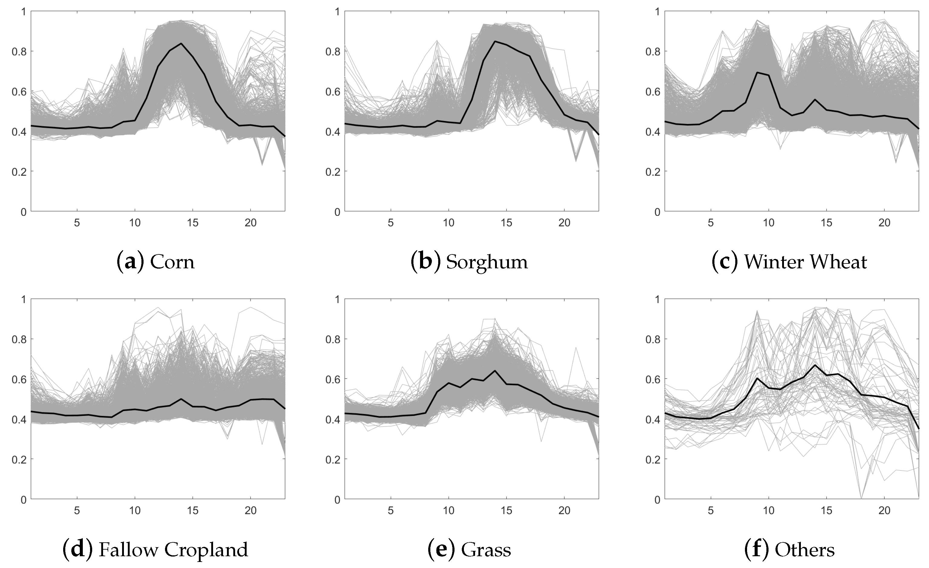
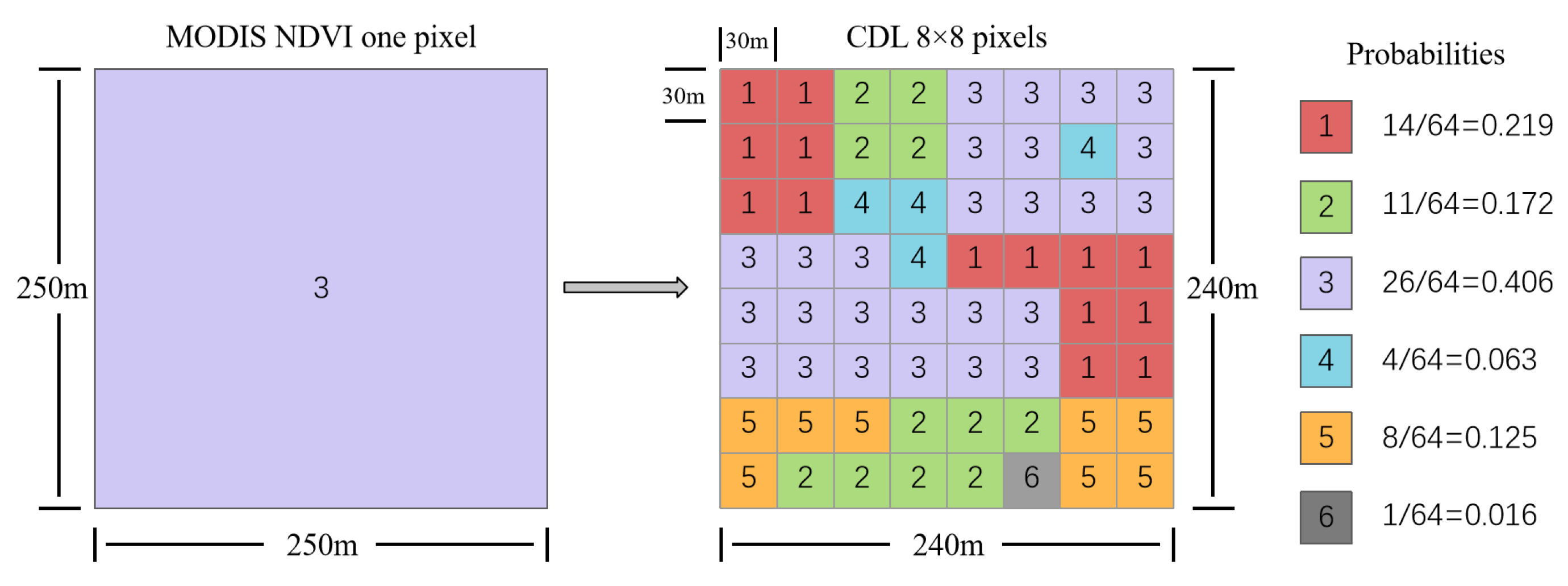
The creation of reference labels of the datasets mainly includes endmember selection and abundance calculation. Firstly, the prior knowledge of the image, CDL, and high-resolution images of Google Earth were used to effectively determine the number of tEMs in the study areas. Secondly, tEMs were mainly obtained from the NDVI profile curves of pixels composed of a single coverage type [6]. We collected uniform and homogeneous pixels representing a similar object in the MODIS NDVI image of the study area, while the pixel reflects the same crop in the neighborhood 8 × 8 patch from the corresponding CDL map. The average values of the homogeneous pixels of the same land cover acquired from different regions were calculated as the final reference tEMs, shown in Figure 3. Thirdly, the reference abundance was mainly calculated based on the CDL map, as shown in Figure 4. For example, a MODIS NDVI pixel with 250 m spatial resolution roughly corresponds to 64 CDL pixels with 30 m spatial resolution, and the probabilities of respective tEMs were calculated, so that the reference abundances corresponding to different land cover types in the study area can be obtained.

3. Methodology

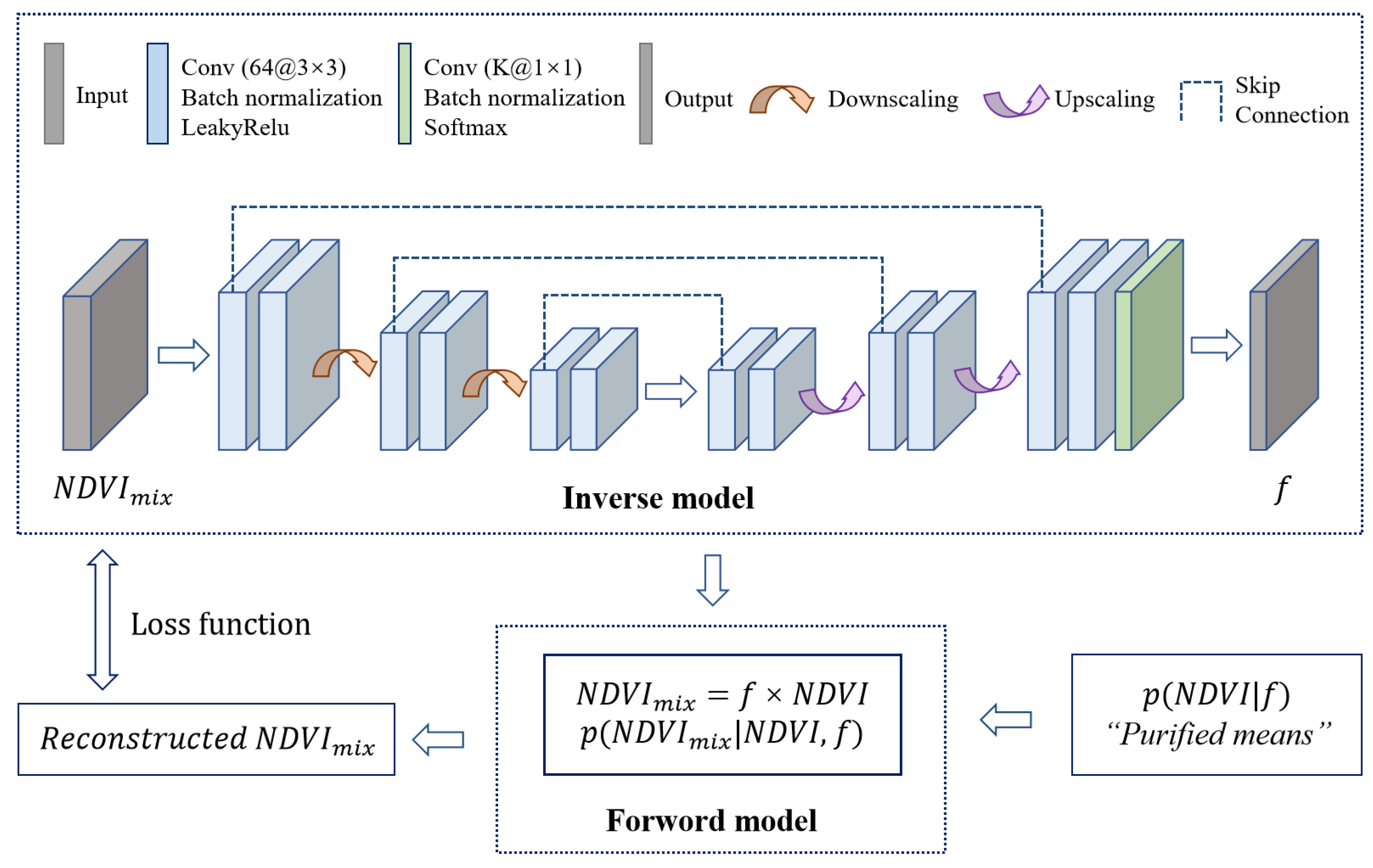
In this section, we propose an temporal unmixing method ST-Bdip based on the Bayesian framework, which innovatively combines the knowledge-driven TMA model and the DL-driven model. This approach considers the influence of spatial correlation and temporal noise variance simultaneously. The specific architecture is depicted in Figure 5. The ST-Bdip method uses the TMA model as the forward model for temporal unmixing, which can mainly be divided into two steps: (1) identify the tEMs of crops; (2) decompose each pixel into crop tEMs and corresponding crop coverage. In addition, the ST-Bdip method uses the inverse model based on U-Net architecture [57] as the principal part for a prior estimate of abundances. The deep image prior model of U-Net architecture can effectively learn the spatial context information, which enhances the representation ability of abundance modeling compared with the traditional non-negative least squares algorithm. Subsequently, the “Purified means” concept and the expectation–maximization (EM) algorithm [58] are used for iterative optimization of tEMs and abundances.

3.1. Temporal Mixture Analysis

With a fully constrained linear TMA, the hybrid pixel can be regarded as the mixture of several specific crops, that is, the multi-temporal NDVI profiles, instead of the traditional reflectance spectra, can be identified for the linear combination of these crop tEMs and the corresponding crop coverages. By selecting the crop types and the number of crop tEMs, TMA can be mathematically modeled as Equation (1).
N D V I m i x = i = 1 N f i × N D V I i + ε
Subject to i = 1 N f i = 1 and f i 0
where N D V I m i x is the NDVI value of a mixed pixel in the time-series image, N is the number of crop tEMs, N D V I i represents the NDVI value of the ith crop tEM, and f i is the fraction of crop tEM i, and ε is the residual. As defined in Equation (2), the abundances of the crop tEMs should satisfy two constraints: (1) non-negative and (2) sum-to-one.
Temporal unmixing aims to extract sequential tEMs N D V I i and estimate the corresponding abundance f i for a given time-series NDVI value N D V I m i x of a mixed pixel. The proposed ST-Bdip method is a deep convolution model based on the Bayesian theorem, which exploits s-temporal deep image prior information. According to the Bayesian theorem, a posteriori distribution of unknown quantities can be established using the original prior distribution of noiseless data, which can be formulated as
p ( N D V I i ,   f i N D V I m i x ) p ( N D V I m i x N D V I i ,   f i ) p ( N D V I i f i )
Then, the posterior distribution can be maximized, i.e., the maximum a posterior (MAP) problem, so that the N D V I i and f i can be estimated. We write N D V I i ,   f i as θ in the following formula:
θ = a r g m a x θ p N D V I i ,   f i N D V I m i x
Theoretically, the maximization of p N D V I i , f i N D V I m i x is also the minimization of the negative log-likelihood representation, i.e.,
θ = a r g m i n θ log p N D V I i ,   f i N D V I m i x a r g m i n θ log p N D V I m i x N D V I i ,   f i log p N D V I i f i log p f i

3.2. Noise Heterogeneity

Generally, most researchers assume that the noise existing in the images is homogeneous noise [59,60]. However, remote sensing time-series images are affected by different levels of noise in both temporal and spectral dimensions due to the illumination variation and difference acquisition time of the dataset. Therefore, we design the model to adapt to the impact of noise heterogeneity in different temporal periods. Based on the least squares optimization model, the term of the data likelihood function is modeled and solved by anisotropic multivariate Gaussian distribution, and the formula p N D V I m i x N D V I i ,   f i can be expressed as follows:
p N D V I m i x N D V I i ,   f i = 1 N e x p N D V I m i x N D V I i f i T Λ 1 N D V I m i x N D V I i f i
where N D V I m i x N D V I i f i T Λ 1 N D V I m i x N D V I i f i represents the reconstruction error of image, and Λ represents the diagonal matrix of noise covariance ε , the formula of which is as follows:
Λ = ε 1 2 ε 2 2 ε T 2
where ε t 2 , t = 1 , 2 , , T represents the noise variance of the tth temporal band. Compared with most existing unmixing methods which assume the same noise level in different temporal or hyperspectral bands, our proposed method considers the heterogeneity of noise in different temporal bands, so as to obtain better noise estimation and unmixing results.

3.3. ST-Bdip Framework

As shown in Figure 5, the U-Net framework combining skip connections in the model is used to efficiently extract the prior spatial information of abundance in the large-scale range area. The model consists of convolution, upsampling, downsampling, and nonlinear activation layers. In addition, the skip connection is used to restrain overfitting and promote the convergence of the model.
The last activation layer of the inverse model is set to the softmax layer because the obtained abundance needs to satisfy the “sum-to-one” and “non-negative” constraints, as shown in Equation (2). In conclusion, the model for estimating the tEMs and abundances contains the following major steps:
  • The estimated abundances are acquired from an inverse model based on the U-Net framework combining skip connections using the MODIS NDVI time-series data.
  • The initial tEMs are obtained based on the VCA algorithm.
  • According to the TMA, the time-series image is reconstructed using the abundances from step 1 and tEMs from step 2.
  • The multivariate Gaussian distribution with an anisotropic covariance matrix to represent the conditional temporal distribution is used. And the Mahalanobis distance-based loss function is calculated for the model optimization to solve the noise heterogeneity effect in remote sensing images. Thus, the model parameters are optimized, and the new abundance is obtained.
  • The “Purified means” method is used to build and further optimize tEMs.
  • The tEMs and abundances are constantly updated through the above step 4 and step 5 until the optimal solution is obtained from EM iteration.

4. Experiments and Results

4.1. Comparison Methods and Parameters

The experiments are conducted with one synthetic dataset and two real MODIS NDVI images. Several traditional and state-of-the-art unmixing algorithms are used for comparison with the proposed ST-Bdip method, e.g., N-FINDR, PPI, VCA-S, VCA-F, uDAs, PnP, and KPmeans. N-FINDR and PPI algorithms are two unsupervised endmember extraction methods widely used in the field of hyperspectral unmixing [61,62,63,64]. The N-FINDR algorithm iteratively searches for endmembers by seeking the direction to maximize the abundance of the selected pixel in the data hyperspace, until all the required endmembers are identified, and then updates the abundances of the selected pixel according to the identified endmembers [15]. Differently, the PPI algorithm directly calculates the pixel purity index of each pixel in the image, selects the pixel with the highest purity index as the endmember, and estimates the corresponding abundances [65]. In addition, both VCA-S and VCA-F methods use the VCA algorithm to extract tEMs, but VCA-S uses the SUnSAL method to estimate the abundance, while VCA-F uses the FCLS method to estimate the abundance. Specifically, SUnSAL is a sparse unmixing algorithm, which initiates the abundance matrix either randomly or based on specific criteria, and subsequently updates the abundance matrix using sparse optimization algorithms [66]. The FCLS method solves the fully constrained least squares equation to minimize the error between the observed data and the linear combination of endmembers, yielding the abundance matrix [22]. Besides conventional unmixing methods, we also compare DL-based approaches that use deep learning techniques to estimate the results in the unmixing application, including uDA and PnP. The uDAs method leverages unsupervised learning algorithms like autoencoders or variational autoencoders to acquire the intrinsic representation of hyperspectral data, enabling the estimation of endmembers and abundances [24]. The PnP method integrates endmember information with prior constraints and employs iterative algorithms to solve optimization problems to obtain abundance maps [31]. KPmeans is a variant of the traditional K-means algorithm that uses kernel functions to process nonlinear data. The conversion data of the K-means clustering algorithm is used to identify the endmembers, and then the corresponding abundances are estimated according to the concept of “Purified means” [17]. The proposed method ST-Bdip refers to the “Purified means” idea of the KPmeans method for iterative updating.
For the proposed ST-Bdip method, we empirically set the number of EM iterations as 50 for simulated data and 1000 for real MODIS NDVI datasets. The experiments are implemented through the MATLAB R2018a platform using codes of the PnP and uDAs methods run with an Intel Xeon Silver 4110 CPU with 2.10 GHz. Other algorithms run on the Pytorch toolbox with an NVIDIA GeForce RTX 2080 Ti GPU.

4.2. Numerical Measures

We employ the following seven evaluation metrics in the experiments: the temporal angle distance (TAD) and the temporal information divergence (TID) to test the performance of tEMs extraction, while the expression formulas are similar to spectral angle distance and the spectral information divergence; the abundance angle distance (AAD), the abundance information divergence (AID), structural similarity (SSIM), and root mean square error between predicted abundances and reference abundance (RMSE-S) to test the performance of abundance estimation; root mean square error of reconstruction image and observation image (RMSE-X) to test the performance of image reconstruction. Their specific representations are as follows:
T A D / A A D = cos 1 x T x ^ / ( x ^   x )
T I D / A I D = D ( x / x ^ ) + D ( x ^ / x )
R M S E = 1 N n = 1 N x n x n ^ 2
where x is the reference tEM, true abundance, or observation HTI image, and x ^ represents reconstruction tEM, reconstruction abundance, or reconstruction HTI image. D ( a / b ) calculates the relative entropy between a and b. SSIM [67] is an evaluation index related to visual effects, which evaluates image quality from contrast, brightness, and structure dimensions. We calculate the SSIM metric using the compare_ssim module from the scikit-image package of Python.

4.3. Test on Simulated Dataset

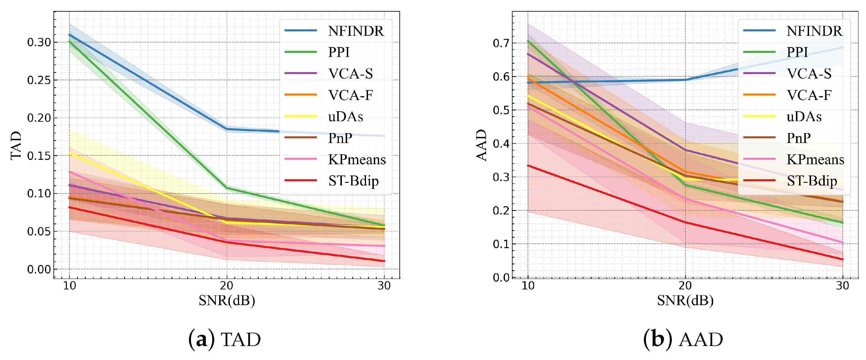
Table 2 quantitatively presents the performance of different unmixing methods using the mean TAD, AAD, TID, AID, and SSIM results of four crops on synthetic data. It is immediately observed that our proposed ST-Bdip method achieves optimal performance under all levels of noise. Table 2 also shows that the larger the SNR of the image, the better the result of unmixing. The SSIM values indicate that the abundance obtained by our proposed ST-Bdip method is most similar to the reference abundance. Different metrics are visually displayed in Figure 6 and Figure 7 with different SNR noises. In Table 2 and Figure 6, we can see that the variance in the ST-Bdip method does not perform the best when the input image has a small SNR, but the overall accuracy is still optimal. In addition, it shows better robustness when the SNR is large, which is similar to other methods. In Figure 7, we can see more intuitively that the ST-Bdip method has the smallest reconstruction error of the abundance, exceeding all other traditional and advanced methods, and the reconstruction errors of the image show few differences in all methods. However, the smaller the error value of the reconstructed image does not signify the better the result due to the existence of the temporal noise.
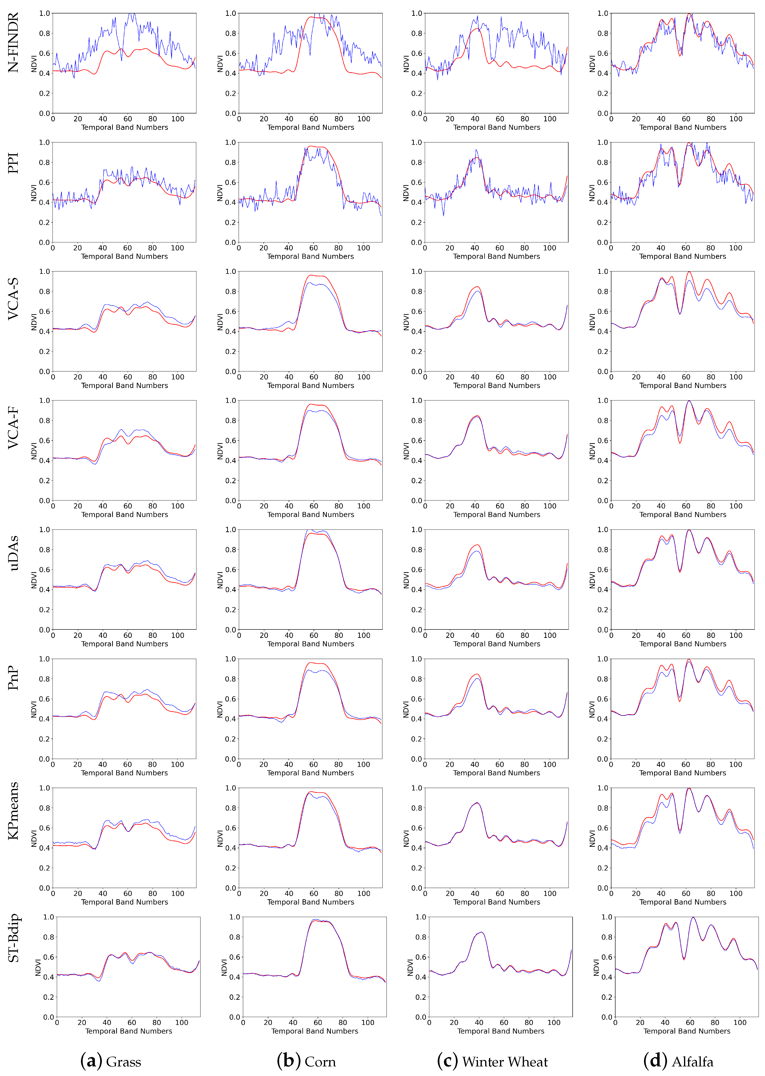
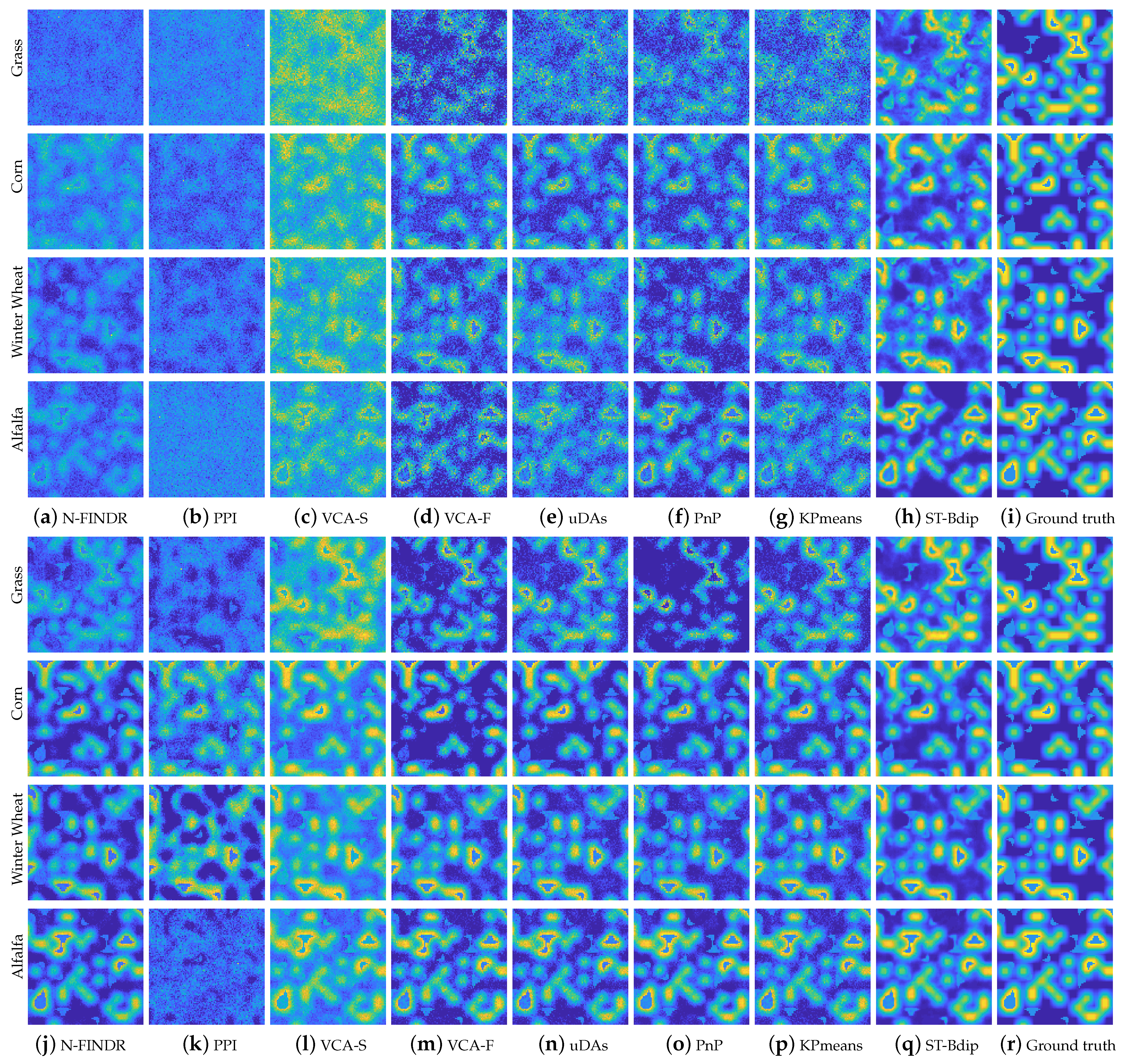
Figure 8 shows the tEM curves of four crops extracted by all methods when SNR noise equals 20 dB. It can be seen that the tEMs extracted by N-FINDR and PPI methods have more noise. Especially, the N-FINDR method deviates more from the reference tEMs of grass, corn, and winter wheat crops. There is little difference between the other methods, and ST-Bdip is closer to the ground truth for all crops. The abundance maps of the four materials for SNR noises equal to 10 dB and 20 dB are shown in Figure 9. We can find that the abundances of the VCA-S method have brighter results because they have no constraint of sum-to-one. In addition, the PPI method fails to unmix this dataset with small SNR, as shown in Figure 9b. Although the result is better when SNR equals 20 dB in Figure 9k, there is still no ideal for “Grass” and “Alfalfa” materials. Overall, the proposed ST-Bdip method shows a minimum salt and pepper noise of abundance, which is closest to the reference abundances.

4.4. Test on MODIS NDVI Dataset

The goal of the experiments is to obtain the abundances at 250 m resolution according to the extracted tEMs of the six main cover types in Scott and Sherman counties, which is helpful for the determination of crop spatial mapping and yield estimation in a higher resolution subsequently. We evaluated the average TAD, AAD, TID, AID, and RMSEs of abundances (represented by RMSE-S) and reconstruction images (represented by RMSE-X) from 20 independent runs by different methods using the MODIS NDVI products in two study areas, as shown in Table 3 and Table 4. The proposed ST-Bdip method shows optimal results in all metrics except RMSE-X. The TAD value of the ST-Bdip method is 0.2300 in Scott County and 0.2612 in Sherman County, and the AAD value is 0.8833 in Scott County and 0.8639 in Sherman County. Empirically, abundance estimation is more valuable and essential than tEM extraction. The results of abundance estimation in Table 3 and Table 4 show that the KPMeans method also has a good performance in Scott County with the AAD value of 0.8888. In Sherman County, the uDAs and KPMeans methods perform well with AAD values of 0.8975 and 0.9071, respectively.
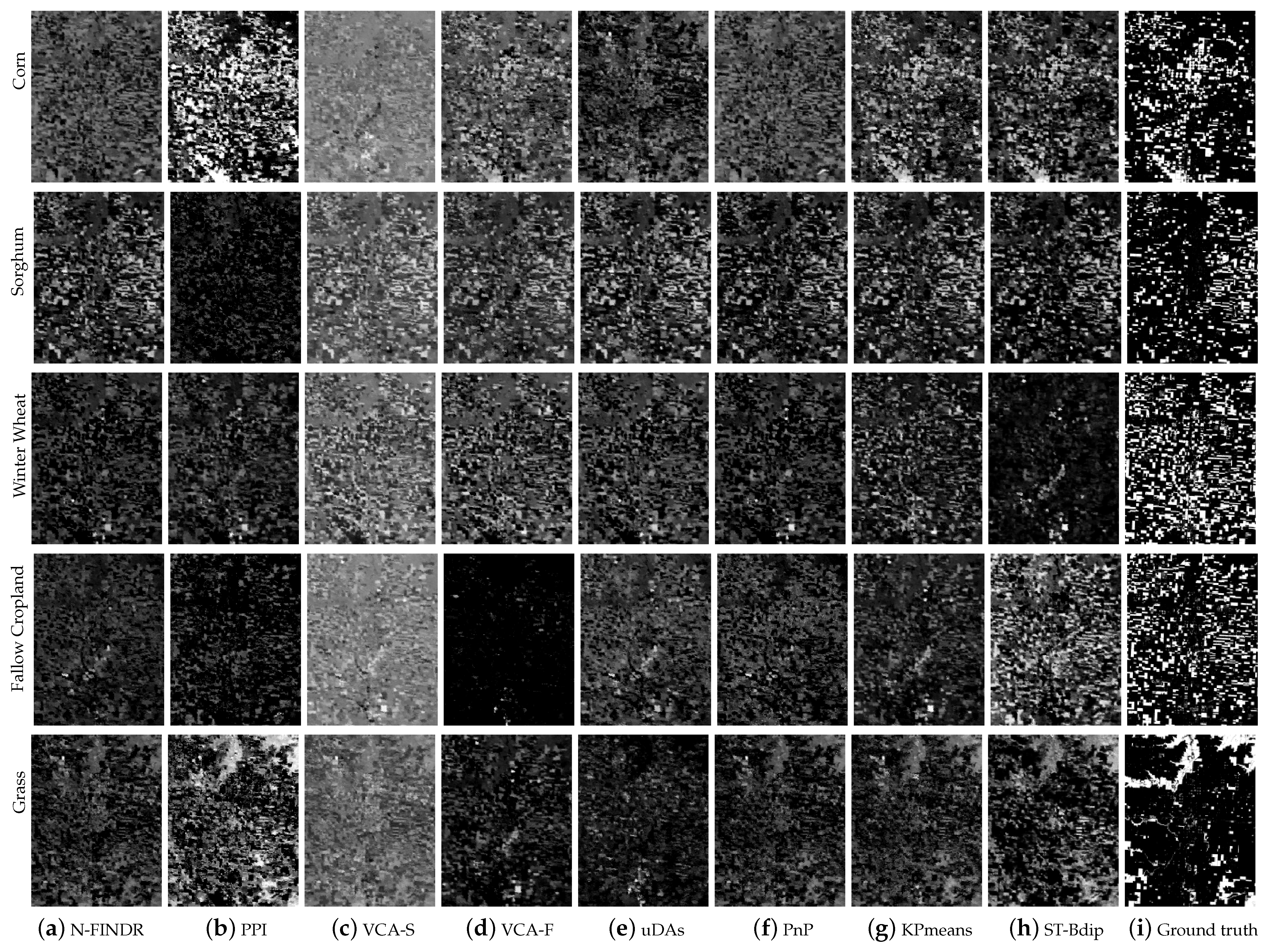
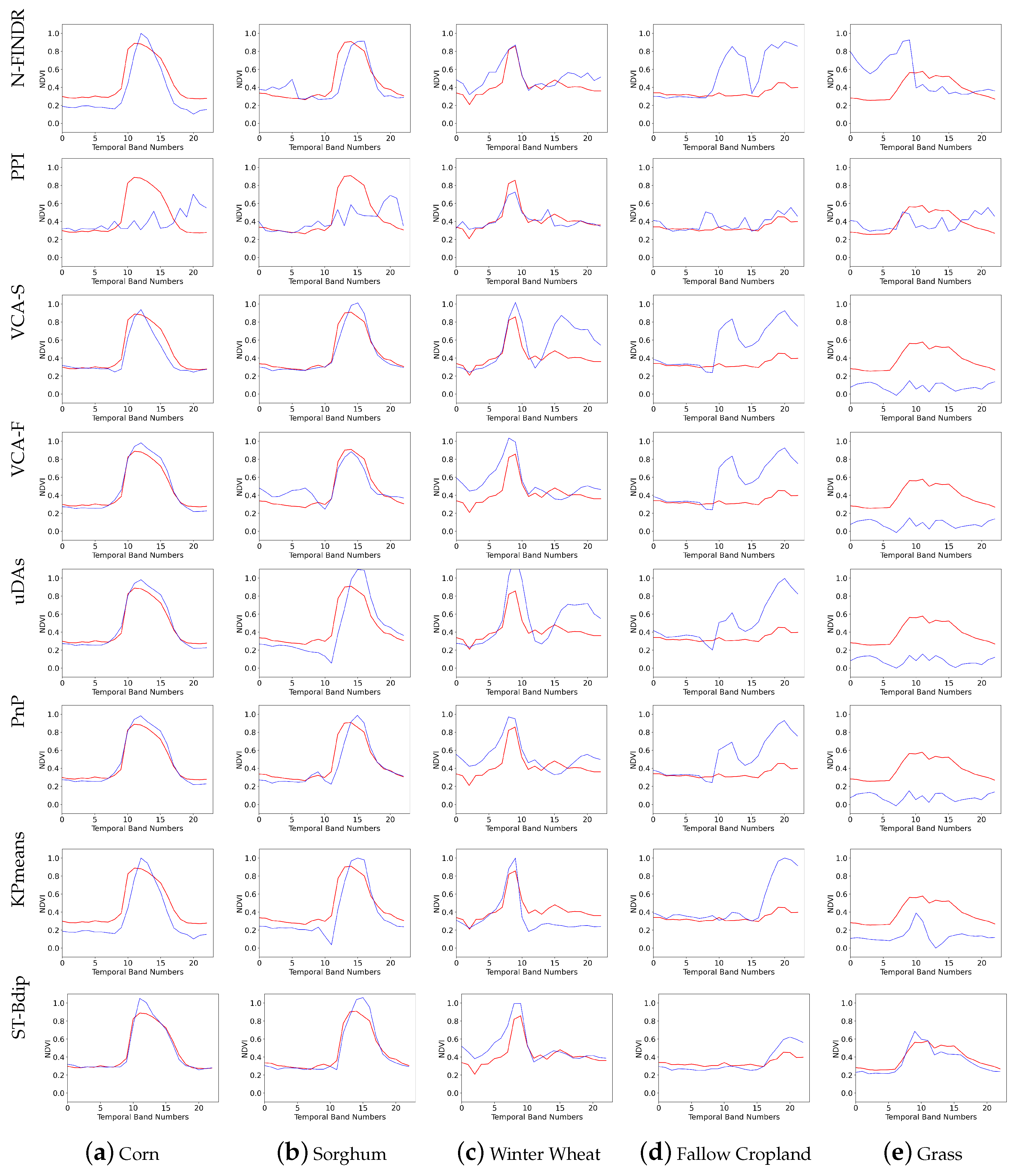
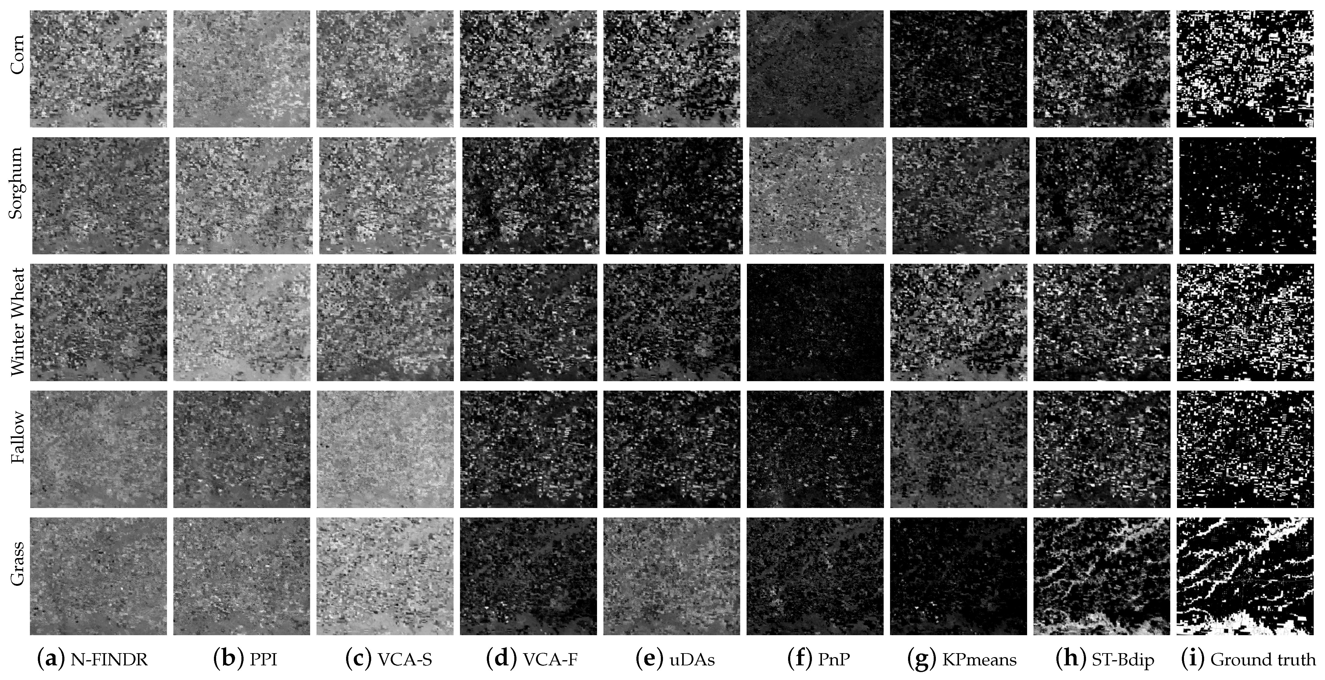
For illustrative purposes, Figure 10, Figure 11, Figure 12 and Figure 13 show some of the classification maps corresponding to the experiments reported in Table 3 and Table 4. There is no exact tEM of the “Other” class while it is calculated by the average of all the other classes, so it does not represent a certain type of land class, and the results do not reflect the superiority of the methods. And five crops (“Corn”, “Sorghum”, “Winter Wheat”, “Fallow Cropland”, and “Grass”) are mainly presented. The comparison of the five tEMs extracted by the eight methods and the reference tEMs (red lines) for Scott and Sherman counties is shown in Figure 10 and Figure 12. Correspondingly, the abundance maps of the two counties are displayed in Figure 11 and Figure 13, respectively. As we can see, compared with simulated data, real MODIS data greatly increase the difficulty of temporal unmixing. The tEMs estimated by the ST-Bdip method are more consistent with the reference tEMs than other methods, which proves the effectiveness of the TMA for the real dataset. Although the NDVI curves of corn and sorghum crops are similar, most methods extract good tEMs of them except PPI, VCA-S, and PnP methods.

5. Discussion

This paper presented a deep s-temporal method ST-Bdip based on the Bayesian framework for temporal unmixing. At present, hyperspectral remote sensing data are mainly used in most crop unmixing applications [8,68]. However, hyperspectral images have some limitations such as data redundancy, small coverage area, and challenges in data acquisition [69]. Given the time-series data as a crucial indicator of crop growth trends, this paper focuses on expanding the endmembers in unmixing from spectral curves to time-series curves and extending the application of unmixing algorithm from hyperspectral images to time-series images, providing different exploration directions to innovatively calculate the individual crop fractions in coarse resolution pixels.

5.1. Advantages of the Proposed ST-Bdip Method

We designed the experiment of traditional and advanced algorithms of hyperspectral unmixing being innovatively applied to the temporal unmixing domain. Different methods show different generalization effects. As shown in Table 2, Table 3 and Table 4, our proposed ST-Bdip method achieves relatively better performance than other comparison methods, both in terms of the extraction of tEMs and the estimation of abundances. Surprisingly, although the “Corn” and “Sorghum” classes show similar growth curves, most methods obtain distinguishable results of them in Figure 10 and Figure 12a,b. It is found that the mistakes of tEMs extraction are mainly concentrated in the “Fallow Cropland” and “Grass” classes. In addition, most existing methods assumed that the noise in the image is homogeneous noise, which cannot reflect the noise distribution in the real remote sensing image. The corresponding solution was designed in our proposed method to solve the problem of heterogeneity noise in the different temporal dimensions. In this paper, three simulated data with different noise levels and two MODIS NDVI data are used to discuss the superiority of the ST-Bdip method in the application of temporal unmixing. The results of the experiments show that most of the traditional and advanced methods have a good performance on the simulated data, and the complexity of real data brought great difficulty to temporal unmixing.
Overall, the abundance maps obtained by the ST-Bdip method are closer to the ground truth maps in terms of both the intense brightness and the structural characteristics, both in Scott County and Sherman County. The proposed ST-Bdip model demonstrates promising results in all materials, particularly in the “Fallow Cropland” class of Scott County and the “Grass” class of Sherman County versus other methods. Essentially, all of the methods misclassify the “Winter Wheat" class of Scott County in the third row of Figure 11. Comparing the CDL map with the predicted abundance maps of this material, we find that most of the highlighted abundances identified by these methods appeared in CDL as the “Alfalfa” class, which is not selected in our experiments because it is a relatively small number in the study areas. It is possible that the extracted tEMs have been biased by these methods, which results in the misclassification of the abundances. Although the uDAs and PnP methods consider the effect of image noise, the results of MODIS data unmixing are still inferior to the proposed ST-Bdip method, which has simulated heterogeneous noise in the temporal dimension.

5.2. Data Complexity Analysis

Figure 8 and Figure 9 reflect that the proposed ST-Bdip method and comparison methods can perform well in the simulation datasets without large deviation. However, the experimental results on the real MODIS data in Figure 10, Figure 11, Figure 12 and Figure 13 show that there are significant differences between different methods and different crops. We conducted a comprehensive analysis and concluded that the above results may be attributed to the complexity of real MODIS data, which can be discussed in the following aspects. First, the simulated datasets contain fewer crop categories and have lower data complexity than the real MODIS data. Second, real MODIS data are susceptible to encountering imbalanced distributions of different crops in the selected study areas, thereby introducing additional complexity to the task of crop unmixing. Third, real MODIS data are usually subject to more complex noise effects, such as Gaussian noise, impulse noise, speckle noise, etc., rather than just the Gaussian noise considered in the simulated data. Considering the above reasons, we implemented the additional data complexity experiment based on the number of crop classes, while the new simulated dataset involves six crop types for comparative assessment. The results are shown in Table 5, in which the results indeed demonstrate that temporal unmixing using time-series images with higher complexity leads to diminished accuracies. This is logical with the prevailing trends in existing applications of MODIS crop unmixing, where experiments are often based on the selection of highly distinguishable crops or a small number of crops [6]. For example, Mutlu Ozdogan used the ICA method for the temporal unmixing of winter crops, summer crops, and other classes, achieving satisfactory results [70].

6. Conclusions

In this paper, we proposed a novel DL-based ST-Bdip method for TMA of time-series images, and the EM algorithm was applied to solve the MAP problem in a Bayesian framework. This method consisted of the U-Net model and the EM algorithm, which were used for the iterative optimization of tEMs and abundances. The 3D convolution layers in the model effectively extracted the information both on the spatial and temporal dimensions. In addition, the noise heterogeneity effect in HTI was addressed by the conditional distribution of temporal observations on the M-distance loss. Three simulated data with different noise levels and two MODIS NDVI data were used for the detailed comparison experiments of seven unmixing algorithms with our proposed method, which proved that the proposed method performs better overall. The exploration of temporal unmixing methods is highly beneficial, which utilizes the important temporal information of crops for timely crop monitoring and environmental, economic, and policy decision-making. However, there are still significant challenges due to the complexity of MODIS data and the similarity of crop growth curves. In the future, we will explore how to simulate data with more accurate noise to be closer to the real data. And the advantages of time-series remote sensing data can be used more effectively when applied to a wider range of fields, particularly in the application of data fusion, where higher resolution remote sensing data (e.g., Landsat) can be synergistically utilized.

Author Contributions

Conceptualization, Y.W. and Y.F.; data collection and data processing, Y.W. and R.Z.; methodology, Y.F.; formal analysis, R.Z.; experiments, Y.W. and R.Z.; writing—original draft preparation, Y.W.; writing—review and editing, Y.W. and L.X.; visualization, Y.W.; supervision, L.X. All authors have read and agreed to the published version of the manuscript.

Funding

This work was supported in part by the National Natural Science Foundation of China under Grant 41501410, University Fund for Distinguished Young Scholars and the Natural Sciences and Engineering Research Council of Canada (NSERC) under Grant RGPIN-2019-06744.

Institutional Review Board Statement

Not applicable.

Informed Consent Statement

Not applicable.

Data Availability Statement

The data presented in this study are available upon request from the corresponding author.

Acknowledgments

The authors would like to thank the reviewers and associate editor for their valuable comments and suggestions to improve the quality of the paper.

Conflicts of Interest

The authors declare no conflict of interest.

References

  1. Cui, J.; Zhang, X.; Luo, M. Combining Linear pixel unmixing and STARFM for spatiotemporal fusion of Gaofen-1 wide field of view imagery and MODIS imagery. Remote Sens. 2018, 10, 1047. [Google Scholar] [CrossRef] [Green Version]
  2. Shen, M.; Tang, Y.; Chen, J.; Zhu, X.; Zheng, Y. Influences of temperature and precipitation before the growing season on spring phenology in grasslands of the central and eastern Qinghai-Tibetan Plateau. Agric. For. Meteorol. 2011, 151, 1711–1722. [Google Scholar] [CrossRef]
  3. Asokan, A.; Anitha, J. Change detection techniques for remote sensing applications: A survey. Earth Sci. Inform. 2019, 12, 143–160. [Google Scholar] [CrossRef]
  4. Goenaga, M.A.; Torres-Madronero, M.C.; Velez-Reyes, M.; Van Bloem, S.J.; Chinea, J.D. Unmixing analysis of a time series of Hyperion images over the Guánica dry forest in Puerto Rico. IEEE J. Sel. Top. Appl. Earth Obs. Remote Sens. 2012, 6, 329–338. [Google Scholar] [CrossRef]
  5. Wang, Q.; Ding, X.; Tong, X.; Atkinson, P.M. Spatio-temporal spectral unmixing of time-series images. Remote Sens. Environ. 2021, 259, 112407. [Google Scholar] [CrossRef]
  6. Lobell, D.B.; Asner, G.P. Cropland distributions from temporal unmixing of MODIS data. Remote Sens. Environ. 2004, 93, 412–422. [Google Scholar] [CrossRef]
  7. Wang, Q.; Peng, K.; Tang, Y.; Tong, X.; Atkinson, P.M. Blocks-removed spatial unmixing for downscaling MODIS images. Remote Sens. Environ. 2021, 256, 112325. [Google Scholar] [CrossRef]
  8. Bioucas-Dias, J.M.; Plaza, A.; Dobigeon, N.; Parente, M.; Du, Q.; Gader, P.; Chanussot, J. Hyperspectral unmixing overview: Geometrical, statistical, and sparse regression-based approaches. IEEE J. Sel. Top. Appl. Earth Obs. Remote Sens. 2012, 5, 354–379. [Google Scholar] [CrossRef] [Green Version]
  9. Foody, G.M. Relating the land-cover composition of mixed pixels to artificial neural network classification output. Photogramm. Eng. Remote Sens. 1996, 62, 491–498. [Google Scholar]
  10. Adams, J.B.; Smith, M.O.; Johnson, P.E. Spectral mixture modeling: A new analysis of rock and soil types at the Viking Lander 1 site. J. Geophys. Res. Solid Earth 1986, 91, 8098–8112. [Google Scholar] [CrossRef]
  11. Liu, J.; Cao, W. Based on linear spectral mixture model (LSMM) Unmixing remote sensing image. In Proceedings of the Third International Conference on Digital Image Processing (ICDIP 2011), Chengdu, China, 15–17 April 2011; SPIE: Paris, France, 2011; Volume 8009, pp. 353–356. [Google Scholar]
  12. Ma, T.; Li, R.; Svenning, J.C.; Song, X. Linear spectral unmixing using endmember coexistence rules and spatial correlation. Int. J. Remote Sens. 2018, 39, 3512–3536. [Google Scholar] [CrossRef]
  13. Tao, X.; Paoletti, M.E.; Han, L.; Wu, Z.; Ren, P.; Plaza, J.; Plaza, A.; Haut, J.M. A New Deep Convolutional Network for Effective Hyperspectral Unmixing. IEEE J. Sel. Top. Appl. Earth Obs. Remote Sens. 2022, 15, 6999–7012. [Google Scholar] [CrossRef]
  14. Nascimento, J.M.; Dias, J.M. Vertex component analysis: A fast algorithm to unmix hyperspectral data. IEEE Trans. Geosci. Remote Sens. 2005, 43, 898–910. [Google Scholar] [CrossRef] [Green Version]
  15. Winter, M.E. N-FINDR: An algorithm for fast autonomous spectral end-member determination in hyperspectral data. In Imaging Spectrometry V; SPIE: Paris, France, 1999; Volume 3753, pp. 266–275. [Google Scholar]
  16. Chang, C.I.; Plaza, A. A fast iterative algorithm for implementation of pixel purity index. IEEE Geosci. Remote Sens. Lett. 2006, 3, 63–67. [Google Scholar] [CrossRef]
  17. Xu, L.; Li, J.; Wong, A.; Peng, J. Kp-means: A clustering algorithm of k “purified” means for hyperspectral endmember estimation. IEEE Geosci. Remote Sens. Lett. 2014, 11, 1787–1791. [Google Scholar]
  18. Zhao, C.; Zhao, G.; Jia, X. Hyperspectral image unmixing based on fast kernel archetypal analysis. IEEE J. Sel. Top. Appl. Earth Obs. Remote Sens. 2016, 10, 331–346. [Google Scholar] [CrossRef]
  19. Feng, X.R.; Li, H.C.; Wang, R.; Du, Q.; Jia, X.; Plaza, A.J. Hyperspectral unmixing based on nonnegative matrix factorization: A comprehensive review. IEEE J. Sel. Top. Appl. Earth Obs. Remote Sens. 2022, 15, 4414–4436. [Google Scholar] [CrossRef]
  20. Heinz, D.C. Fully constrained least squares linear spectral mixture analysis method for material quantification in hyperspectral imagery. IEEE Trans. Geosci. Remote Sens. 2001, 39, 529–545. [Google Scholar] [CrossRef] [Green Version]
  21. Bioucas-Dias, J.M.; Figueiredo, M.A. Alternating direction algorithms for constrained sparse regression: Application to hyperspectral unmixing. In Proceedings of the 2nd Workshop on Hyperspectral Image and Signal Processing: Evolution in Remote Sensing, Reykjavik, Iceland, 14–16 June 2010; IEEE: New York, NY, USA, 2010; pp. 1–4. [Google Scholar]
  22. Xu, X.; Shi, Z.; Pan, B. A supervised abundance estimation method for hyperspectral unmixing. Remote Sens. Lett. 2018, 9, 383–392. [Google Scholar] [CrossRef]
  23. Guo, R.; Wang, W.; Qi, H. Hyperspectral image unmixing using autoencoder cascade. In Proceedings of the 7th Workshop on Hyperspectral Image and Signal Processing: Evolution in Remote Sensing (WHISPERS), Tokyo, Japan, 2–5 June 2015; IEEE: New York, NY, USA, 2015; pp. 1–4. [Google Scholar]
  24. Qu, Y.; Qi, H. UDAS: An untied denoising autoencoder with sparsity for spectral unmixing. IEEE Trans. Geosci. Remote Sens. 2018, 57, 1698–1712. [Google Scholar] [CrossRef]
  25. Gao, L.; Han, Z.; Hong, D.; Zhang, B.; Chanussot, J. CyCU-Net: Cycle-consistency unmixing network by learning cascaded autoencoders. IEEE Trans. Geosci. Remote Sens. 2021, 60, 1–14. [Google Scholar] [CrossRef]
  26. Qi, L.; Li, J.; Wang, Y.; Lei, M.; Gao, X. Deep spectral convolution network for hyperspectral image unmixing with spectral library. Signal Process. 2020, 176, 107672. [Google Scholar] [CrossRef]
  27. Zhang, X.; Sun, Y.; Zhang, J.; Wu, P.; Jiao, L. Hyperspectral unmixing via deep convolutional neural networks. IEEE Geosci. Remote Sens. Lett. 2018, 15, 1755–1759. [Google Scholar] [CrossRef]
  28. Palsson, B.; Ulfarsson, M.O.; Sveinsson, J.R. Convolutional autoencoder for spectral–spatial hyperspectral unmixing. IEEE Trans. Geosci. Remote Sens. 2020, 59, 535–549. [Google Scholar] [CrossRef]
  29. Yan, C.; Fan, X.; Fan, J.; Wang, N. Improved U-Net remote sensing classification algorithm based on Multi-Feature Fusion Perception. Remote Sens. 2022, 14, 1118. [Google Scholar] [CrossRef]
  30. He, N.; Fang, L.; Plaza, A. Hybrid first and second order attention Unet for building segmentation in remote sensing images. Sci. China Inf. Sci. 2020, 63, 140305. [Google Scholar] [CrossRef] [Green Version]
  31. Zhao, M.; Wang, X.; Chen, J.; Chen, W. A Plug-and-Play Priors Framework for Hyperspectral Unmixing. IEEE Trans. Geosci. Remote Sens. 2021, 60, 5501213. [Google Scholar] [CrossRef]
  32. Diao, C.; Wang, L. Temporal partial unmixing of exotic salt cedar using Landsat time series. Remote Sens. Lett. 2016, 7, 466–475. [Google Scholar] [CrossRef]
  33. Borsoi, R.A.; Imbiriba, T.; Bermudez, J.C.M.; Richard, C.; Chanussot, J.; Drumetz, L.; Tourneret, J.Y.; Zare, A.; Jutten, C. Spectral variability in hyperspectral data unmixing: A comprehensive review. IEEE Geosci. Remote Sens. Mag. 2021, 9, 223–270. [Google Scholar] [CrossRef]
  34. Hong, D.; Gao, L.; Yao, J.; Yokoya, N.; Chanussot, J.; Heiden, U.; Zhang, B. Endmember-guided unmixing network (EGU-Net): A general deep learning framework for self-supervised hyperspectral unmixing. IEEE Trans. Neural Netw. Learn. Syst. 2021, 33, 6518–6531. [Google Scholar] [CrossRef]
  35. Su, Y.; Li, J.; Plaza, A.; Marinoni, A.; Gamba, P.; Chakravortty, S. Daen: Deep autoencoder networks for hyperspectral unmixing. IEEE Trans. Geosci. Remote Sens. 2019, 57, 4309–4321. [Google Scholar] [CrossRef]
  36. Chen, Y.; Song, X.; Wang, S.; Huang, J.; Mansaray, L.R. Impacts of spatial heterogeneity on crop area mapping in Canada using MODIS data. ISPRS J. Photogramm. Remote Sens. 2016, 119, 451–461. [Google Scholar] [CrossRef]
  37. Marchane, A.; Jarlan, L.; Hanich, L.; Boudhar, A.; Gascoin, S.; Tavernier, A.; Filali, N.; Le Page, M.; Hagolle, O.; Berjamy, B. Assessment of daily MODIS snow cover products to monitor snow cover dynamics over the Moroccan Atlas mountain range. Remote Sens. Environ. 2015, 160, 72–86. [Google Scholar] [CrossRef]
  38. Portillo-Quintero, C.; Sanchez, A.; Valbuena, C.; Gonzalez, Y.; Larreal, J. Forest cover and deforestation patterns in the Northern Andes (Lake Maracaibo Basin): A synoptic assessment using MODIS and Landsat imagery. Appl. Geogr. 2012, 35, 152–163. [Google Scholar] [CrossRef]
  39. Lloyd, D. A phenological classification of terrestrial vegetation cover using shortwave vegetation index imagery. Remote Sens. 1990, 11, 2269–2279. [Google Scholar] [CrossRef]
  40. Wardlow, B.D.; Egbert, S.L.; Kastens, J.H. Analysis of time-series MODIS 250 m vegetation index data for crop classification in the US Central Great Plains. Remote Sens. Environ. 2007, 108, 290–310. [Google Scholar] [CrossRef] [Green Version]
  41. Son, N.T.; Chen, C.F.; Chen, C.R.; Duc, H.N.; Chang, L.Y. A phenology-based classification of time-series MODIS data for rice crop monitoring in Mekong Delta, Vietnam. Remote Sens. 2013, 6, 135–156. [Google Scholar] [CrossRef] [Green Version]
  42. Sun, C.; Li, J.; Cao, L.; Liu, Y.; Jin, S.; Zhao, B. Evaluation of Vegetation Index-Based Curve Fitting Models for Accurate Classification of Salt Marsh Vegetation Using Sentinel-2 Time-Series. Sensors 2020, 20, 5551. [Google Scholar] [CrossRef]
  43. Piwowar, J.M.; Peddle, D.R.; LeDrew, E.F. Temporal mixture analysis of arctic sea ice imagery: A new approach for monitoring environmental change. Remote Sens. Environ. 1998, 63, 195–207. [Google Scholar] [CrossRef]
  44. Yang, F.; Matsushita, B.; Fukushima, T.; Yang, W. Temporal mixture analysis for estimating impervious surface area from multi-temporal MODIS NDVI data in Japan. ISPRS J. Photogramm. Remote Sens. 2012, 72, 90–98. [Google Scholar] [CrossRef] [Green Version]
  45. Li, W.; Wu, C. Phenology-based temporal mixture analysis for estimating large-scale impervious surface distributions. Int. J. Remote Sens. 2014, 35, 779–795. [Google Scholar] [CrossRef]
  46. Zhuo, L.; Shi, Q.; Tao, H.; Zheng, J.; Li, Q. An improved temporal mixture analysis unmixing method for estimating impervious surface area based on MODIS and DMSP-OLS data. ISPRS J. Photogramm. Remote Sens. 2018, 142, 64–77. [Google Scholar] [CrossRef]
  47. Torres-Madronero, M.C.; Velez-Reyes, M.; Van Bloem, S.J.; Chinea, J.D. Multi-temporal unmixing analysis of Hyperion images over the Guanica Dry Forest. In Proceedings of the 3rd Workshop on Hyperspectral Image and Signal Processing: Evolution in Remote Sensing (WHISPERS), Lisbon, Portugal, 6–9 June 2011; IEEE: New York, NY, USA, 2011; pp. 1–4. [Google Scholar]
  48. Chi, J.; Kim, H.C.; Kang, S.H. Machine learning-based temporal mixture analysis of hypertemporal Antarctic sea ice data. Remote Sens. Lett. 2016, 7, 190–199. [Google Scholar] [CrossRef]
  49. Liu, Z.; Hu, Q.; Tan, J.; Zou, J. Regional scale mapping of fractional rice cropping change using a phenology-based temporal mixture analysis. Int. J. Remote Sens. 2019, 40, 2703–2716. [Google Scholar] [CrossRef]
  50. Bruce, L.M.; Mathur, A.; Byrd, J.D., Jr. Denoising and wavelet-based feature extraction of MODIS multi-temporal vegetation signatures. GIScience Remote Sens. 2006, 43, 67–77. [Google Scholar] [CrossRef]
  51. Hermance, J.F.; Jacob, R.W.; Bradley, B.A.; Mustard, J.F. Extracting phenological signals from multiyear AVHRR NDVI time series: Framework for applying high-order annual splines with roughness damping. IEEE Trans. Geosci. Remote Sens. 2007, 45, 3264–3276. [Google Scholar] [CrossRef]
  52. Liang, S.z.; Ma, W.d.; Sui, X.y.; Yao, H.m.; Li, H.z.; Liu, T.; Hou, X.h.; Wang, M. Extracting the spatiotemporal pattern of cropping systems from NDVI time series using a combination of the spline and HANTS Algorithms: A case study for Shandong Province. Can. J. Remote Sens. 2017, 43, 1–15. [Google Scholar] [CrossRef]
  53. Shou-Zhen, L.; Peng, S.; Qian-Guo, X. A comparison between the algorithms for removing cloud pixel from MODIS NDVI time series data. Remote Sens. Nat. Resour. 2011, 23, 33–36. [Google Scholar]
  54. Shao, Y.; Lunetta, R.S.; Wheeler, B.; Iiames, J.S.; Campbell, J.B. An evaluation of time-series smoothing algorithms for land-cover classifications using MODIS-NDVI multi-temporal data. Remote Sens. Environ. 2016, 174, 258–265. [Google Scholar] [CrossRef]
  55. Zhong, L.; Hu, L.; Zhou, H.; Tao, X. Deep learning based winter wheat mapping using statistical data as ground references in Kansas and northern Texas, US. Remote Sens. Environ. 2019, 233, 111411. [Google Scholar] [CrossRef]
  56. Chen, Y.; Lu, D.; Moran, E.; Batistella, M.; Dutra, L.V.; Sanches, I.D.; da Silva, R.F.B.; Huang, J.; Luiz, A.J.B.; de Oliveira, M.A.F. Mapping croplands, cropping patterns, and crop types using MODIS time-series data. Int. J. Appl. Earth Obs. Geoinf. 2018, 69, 133–147. [Google Scholar] [CrossRef]
  57. Barkau, R.L. UNET: One-Dimensional Unsteady Flow through a Full Network of Open Channels. User’s Manual; Technical Report; Hydrologic Engineering Center: Davis, CA, USA, 1996. [Google Scholar]
  58. Ng, S.K.; Krishnan, T.; McLachlan, G.J. The EM algorithm. In Handbook of Computational Statistics: Concepts and Methods; Springer: Berlin/Heidelberg, Germany, 2012; pp. 139–172. [Google Scholar]
  59. Lebrun, M.; Buades, A.; Morel, J.M. A nonlocal Bayesian image denoising algorithm. SIAM J. Imaging Sci. 2013, 6, 1665–1688. [Google Scholar] [CrossRef]
  60. Nascimento, J.M.; Bioucas-Dias, J.M. Nonlinear mixture model for hyperspectral unmixing. In Image and Signal Processing for Remote Sensing XV; SPIE: Paris, France, 2009; Volume 7477, pp. 157–164. [Google Scholar]
  61. Winter, M.E. A proof of the N-FINDR algorithm for the automated detection of endmembers in a hyperspectral image. In Algorithms and Technologies for Multispectral, Hyperspectral, and Ultraspectral Imagery X; SPIE: Paris, France, 2004; Volume 5425, pp. 31–41. [Google Scholar]
  62. Keleşoğlu, G.; Ertürk, A.; Erten, E. Analysis of mucilage levels build up in the sea of Marmara based on unsupervised unmixing of worldview-3 data. In Proceedings of the IEEE Mediterranean and Middle-East Geoscience and Remote Sensing Symposium (M2GARSS), Istanbul, Turkey, 7–9 March 2022; IEEE: New York, NY, USA, 2022; pp. 102–105. [Google Scholar]
  63. Ishidoshiro, N.; Yamaguchi, Y.; Noda, S.; Asano, Y.; Kondo, T.; Kawakami, Y.; Mitsuishi, M.; Nakamura, H. Geological mapping by combining spectral unmixing and cluster analysis for hyperspectral data. Int. Arch. Photogramm. Remote Sens. Spat. Inf. Sci. 2016, 41, 431–435. [Google Scholar] [CrossRef] [Green Version]
  64. Lopez, A.C.C.; Mora, M.M.G.; Torres-Madroñero, M.C.; Velez-Reyes, M. Using hyperspectral unmixing for the analysis of very high spatial resolution hyperspectral imagery. In Algorithms, Technologies, and Applications for Multispectral and Hyperspectral Imaging XXIX; SPIE: Paris, France, 2023; Volume 12519, pp. 277–284. [Google Scholar]
  65. Martínez, P.J.; Pérez, R.M.; Plaza, A.; Aguilar, P.L.; Cantero, M.C.; Plaza, J. Endmember extraction algorithms from hyperspectral images. Ann. Geophys. 2006, 49, 93–101. [Google Scholar] [CrossRef]
  66. Wang, R.; Li, H.C.; Liao, W.; Pižurica, A. Double reweighted sparse regression for hyperspectral unmixing. In Proceedings of the IEEE International Geoscience and Remote Sensing Symposium (IGARSS), Beijing, China, 10–15 July 2016; IEEE: New York, NY, USA, 2016; pp. 6986–6989. [Google Scholar]
  67. Horé, A.; Ziou, D. Image Quality Metrics: PSNR vs. SSIM. In Proceedings of the 20th International Conference on Pattern Recognition, Istanbul, Turkey, 23–26 August 2010; pp. 2366–2369. [Google Scholar] [CrossRef]
  68. Palsson, B.; Sigurdsson, J.; Sveinsson, J.R.; Ulfarsson, M.O. Hyperspectral unmixing using a neural network autoencoder. IEEE Access 2018, 6, 25646–25656. [Google Scholar] [CrossRef]
  69. Sun, W.; Yang, G.; Peng, J.; Meng, X.; He, K.; Li, W.; Li, H.C.; Du, Q. A multiscale spectral features graph fusion method for hyperspectral band selection. IEEE Trans. Geosci. Remote Sens. 2021, 60, 5513712. [Google Scholar] [CrossRef]
  70. Ozdogan, M. The spatial distribution of crop types from MODIS data: Temporal unmixing using Independent Component Analysis. Remote Sens. Environ. 2010, 114, 1190–1204. [Google Scholar] [CrossRef]
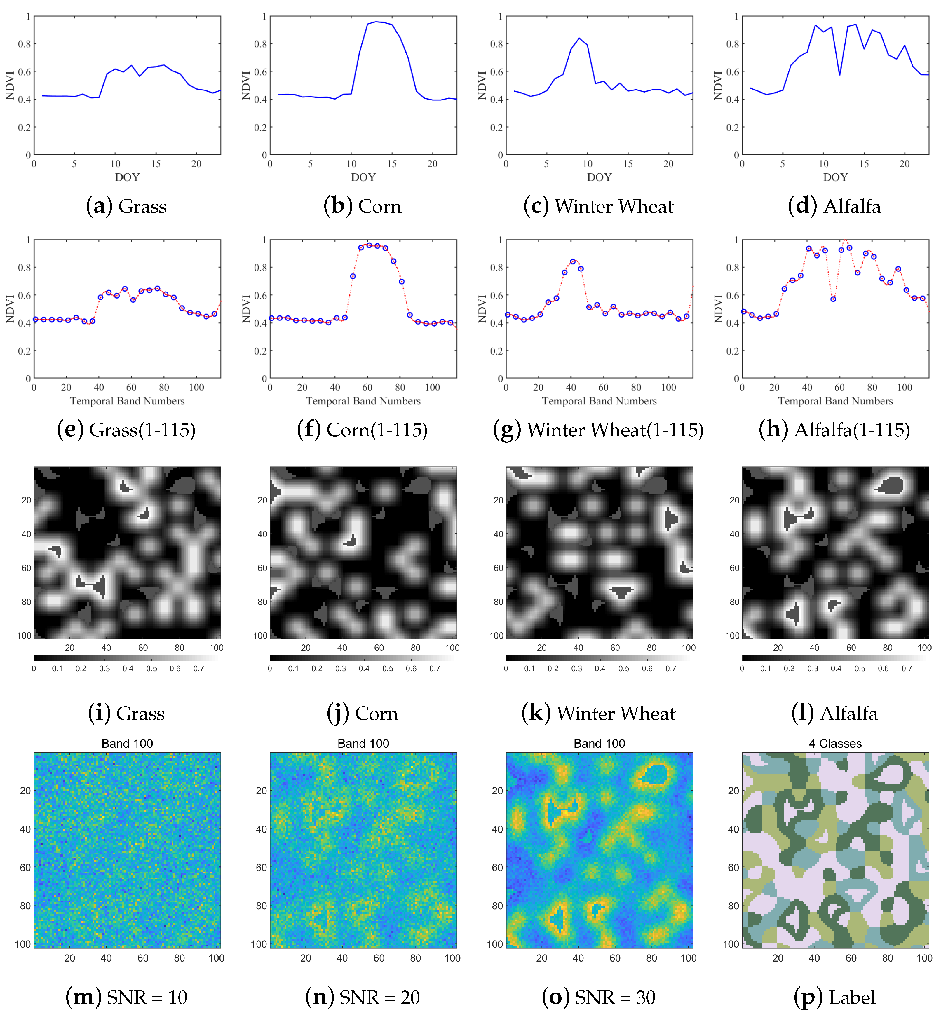
Figure 1. (ad) Illustration of four crop tEMs selected from MODIS NDVI data. (eh) Illustration of four simulated crop tEMs with 115 bands generated by the spline interpolation method. (il) Illustration of four simulated abundance maps with the size of 102 × 102 pixels. (mo) Illustration the noisy images by randomly selected 100th band of simulated data at different SNR levels. (p) Display of the hard label of the simulated datasets.
Remotesensing 15 03782 g001
Figure 2. Locations and label maps of two study areas. (a) Overall area: Kansas; (b) Sherman County; (c) Scott County.
Remotesensing 15 03782 g002
Figure 3. The selection method of reference tEMs. In each subgraph, grey lines represent the temporal curves of the homogeneous pixels of the same cropland type, and the black line represents the average temporal curve of all these homogeneous pixels.
Remotesensing 15 03782 g003
Figure 4. The calculation method of reference abundances. A MODIS NDVI pixel with 250 m spatial resolution roughly corresponds to 64 CDL pixels with 30 m spatial resolution, and the probability of each tEM is calculated, so that the reference abundances corresponding to different land cover types in the study area can be obtained.
Remotesensing 15 03782 g004
Figure 5. Model flowchart. N D V I m i x represents input time-series data, and each pixel expresses an exclusive NDVI profile curve. f represents the abundances estimated by the inverse model, the channel number of which symbolizes the number of crop categories. The “Inverse model” part is based on a U-Net model to learn the spatial correlation of the abundance field by DIP p ( f ) . The crop tEM N D V I is estimated using the “Purified means” method, which is integrated into the Bayesian framework when the abundance p ( N D V I | f ) is given. Then, TMA is employed as the “Forward model”, in which the abundance f estimated by the U-Net framework and the tEM N D V I are used to obtain the reconstructed image R e c o n s t r u c t e d N D V I m i x , and the “Loss function” is calculated to optimize the model parameters by backpropagation. Finally, within the threshold or iterations, the tEM N D V I and abundance f are updated continuously by combining the EM iteration to achieve the final results.
Remotesensing 15 03782 g005
Figure 6. TAD and AAD metrics of simulated datasets with 10 dB to 30 dB SNRs. Different colored solid lines represent different methods, and their adjacent low saturation areas represent the corresponding variance.
Remotesensing 15 03782 g006
Figure 7. The RMSE-S between the predicted abundances and the true abundance and the RMSE-X between the reconstructed images and the observed image of different methods for simulated datasets with 10 dB to 30 dB SNRs.
Remotesensing 15 03782 g007
Figure 8. Extracted tEM curves (interpolation NDVI curves) comparison between the different methods (blue lines) and the corresponding ground truths (red lines) on the simulated dataset when SNR equals 20 dB. Column (ad) displays the “Grass”, “Corn”, “Winter Wheat”, and “Other” crops, respectively.
Remotesensing 15 03782 g008
Figure 9. The abundance maps achieved by different methods on four tEMs on the simulated dataset when SNR equals 10 dB and 20 dB. Columns (ah) represent the results for the simulated data with SNR equals 10 dB, and columns (jq) represent the results for the simulated data with SNR equals 20 dB. Columns (i,r) show the reference abundance maps of four materials. Brighter pixels indicate high abundance while darker pixels indicate low abundance. It shows that the ST-Bdip method is more capable of generating abundance maps that are close to the ground truth maps in terms of both the intense brightness and the structural characteristics.
Remotesensing 15 03782 g009
Figure 10. Extracted tEM curves comparison between the different methods (blue lines) and the corresponding ground truths (red lines) on the Scott County. Column (ae) displays the “Corn”, “Sorghum”, “Winter Wheat”, “Fallow Cropland” and “Grass” crops, respectively.
Remotesensing 15 03782 g010
Figure 11. The abundance maps achieved by different methods on five tEMs (corn, sorghum, winter wheat, fallow cropland, and grass, respectively) from the top row to bottom row for temporal NDVI data in Scott County. Column (ah) display the results of “N-FINDR”, “PPI”, “VCA-S”, “VCA-F”, “uDAs”, “PnP”, “KPmeans”, and “ST-Bdip” methods, respectively. And column (i) displays the reference abundances.
Remotesensing 15 03782 g011
Figure 12. Extracted tEM curves comparison between the different methods (blue lines) and the corresponding ground truths (red lines) on the Sherman County. Column (ae) display the “Corn”, “Sorghum”, “Winter Wheat”, “Fallow Cropland”, and “Grass” crops, respectively.
Remotesensing 15 03782 g012
Figure 13. The abundance maps achieved by different methods on five tEMs (corn, sorghum, winter wheat, fallow cropland, and grass), respectively, from the top row to bottom row for temporal NDVI data in Sherman County. Column (ah) display the results of “N-FINDR”, “PPI”, “VCA-S”, “VCA-F”, “uDAs”, “PnP”, “KPmeans”, and “ST-Bdip” methods, respectively. And column (i) displays the reference abundances.
Remotesensing 15 03782 g013
Table 1. The data and pertinent information utilized in this study.
DataSpatial ResolutionTime PeriodProjectionDownload Source
MOD13Q1250 m2018/01/01Sinusoidal projectionhttps://ladsweb.modaps.eosdis.nasa.gov/ (accessed on 1 June 2023)
CDL30 m2018–2018/12/31Albers Equal Area Conic projectionhttps://nassgeodata.gmu.edu/CropScape/ (accessed on 1 June 2023)
Table 2. Mean TAD, AAD, TID, AID, 1-SSIM, and the variances of them obtained from 10 independent runs by different methods using the simulated data over SNR from 10 to 30 dB. The best results are in bold.
SNR = 10, 4 tEMs, 102 × 102 size, 115 bands
MethodTADAADTIDAID1-SSIM
N-FINDR0.3096 ± 0.020.5818 ± 0.030.1320 ± 0.024.5547 ± 0.360.5473
PPI0.3006 ± 0.010.7055 ± 0.030.1101 ± 0.015.5562 ± 0.330.7019
VCA-S0.1108 ± 0.030.6669 ± 0.180.0170 ± 0.015.1622 ± 4.000.4683
VCA-F0.0953 ± 0.040.5936 ± 0.130.0137 ± 0.016.3974 ± 3.470.3889
uDAs0.1531 ± 0.040.5420 ± 0.090.0355 ± 0.024.1086 ± 1.220.3990
PnP0.0936 ± 0.040.5186 ± 0.130.0123 ± 0.014.4523 ± 1.970.2872
KPmeans0.1286 ± 0.040.5098 ± 0.090.0241 ± 0.013.8117 ± 1.300.3343
ST-Bdip0.0816 ± 0.040.3339 ± 0.150.0110 ± 0.012.1410 ± 1.100.1387
SNR = 20, 4 tEMs, 102 × 102 size, 115 bands
MethodTADAADTIDAID1-SSIM
N-FINDR0.1849 ± 0.010.5896 ± 0.050.0404 ± 0.005.0966 ± 0.720.5711
PPI0.1073 ± 0.010.2756 ± 0.020.0132 ± 0.001.7968 ± 0.250.1669
VCA-S0.0672 ± 0.030.3803 ± 0.190.0056 ± 0.001.7978 ± 2.550.1965
VCA-F0.0648 ± 0.030.3151 ± 0.100.0052 ± 0.012.0104 ± 1.230.1961
uDAs0.0612 ± 0.040.2932 ± 0.120.0072 ± 0.011.9552 ± 1.680.1531
PnP0.0655 ± 0.030.3035 ± 0.100.0055 ± 0.012.1320 ± 1.340.1763
KPmeans0.0376 ± 0.020.2341 ± 0.130.0025 ± 0.001.5301 ± 1.880.1217
ST-Bdip0.0354 ± 0.020.1640 ± 0.080.0032 ± 0.001.0483 ± 0.530.0658
SNR = 30, 4 tEMs, 102 × 102 size, 115 bands
MethodTADAADTIDAID1-SSIM
N-FINDR0.1758 ± 0.000.6864 ± 0.080.0391 ± 0.009.4483 ± 2.970.4656
PPI0.0577 ± 0.000.1632 ± 0.030.0036 ± 0.000.5543 ± 0.240.0777
VCA-S0.0546 ± 0.020.2612 ± 0.180.0036 ± 0.001.0269 ± 2.360.1553
VCA-F0.0537 ± 0.020.2264 ± 0.070.0036 ± 0.001.2240 ± 0.870.1064
uDAs0.0554 ± 0.030.2874 ± 0.120.0053 ± 0.011.8998 ± 1.790.1278
PnP0.0530 ± 0.010.2255 ± 0.050.0031 ± 0.001.2114 ± 0.570.1435
KPmeans0.0306 ± 0.010.1044 ± 0.040.0013 ± 0.000.3667 ± 0.280.0539
ST-Bdip0.0107 ± 0.010.0536 ± 0.020.0003 ± 0.000.2663 ± 0.210.0120
Table 3. Mean TAD, AAD, TID, AID, their variances, the RMSE-S and RMSE-X obtained from 20 independent runs by different methods using the MODIS NDVI products in Scott County. The best results are in bold.
MethodsTADAADTIDAIDRMSE-SRMSE-X
N-FINDR0.2757 ± 0.050.9939 ± 0.040.3208 ± 0.0115.0797 ± 0.990.29110.0576
PPI0.3007 ± 0.061.0194 ± 0.090.9141 ± 0.4416.3344 ± 2.420.29690.0671
VCA-S0.2463 ± 0.041.0092 ± 0.090.0796 ± 0.0349.9739 ± 16.470.28650.0359
VCA-F0.2541 ± 0.050.9612 ± 0.050.0832 ± 0.0314.8227 ± 1.900.30190.0473
uDAs0.2943 ± 0.090.9452 ± 0.070.3228 ± 0.5515.1977 ± 2.020.30820.0477
PnP0.2644 ± 0.080.9668 ± 0.090.0871 ± 0.0516.2128 ± 3.310.28040.0559
KPmeans0.2557 ± 0.060.8888 ± 0.050.1128 ± 0.1313.6755 ± 0.780.26060.0403
ST-Bdip0.2300 ± 0.050.8833 ± 0.060.0710 ± 0.0513.1397 ± 1.210.23820.0451
Table 4. Mean TAD, AAD, TID, AID, their variances, the RMSE-S and RMSE-X obtained from 20 independent runs by different methods using the MODIS NDVI products in Sherman County. The best results are in bold.
MethodsTADAADTIDAIDRMSE-SRMSE-X
N-FINDR0.3067 ± 0.021.0186 ± 0.080.1263 ± 0.0115.6274 ± 2.610.31030.0795
PPI0.3185 ± 0.021.0446 ± 0.090.1407 ± 0.0217.5854 ± 8.490.32010.1177
VCA-S0.3312 ± 0.101.0687 ± 0.130.1558 ± 0.1147.1089 ± 26.490.33480.0415
VCA-F0.3173 ± 0.070.9284 ± 0.060.1431 ± 0.0614.5976 ± 1.160.27810.0543
uDAs0.3296 ± 0.070.8975 ± 0.050.7204 ± 0.7513.6823 ± 1.090.27990.0516
PnP0.2915 ± 0.020.9298 ± 0.020.1201 ± 0.0116.6188 ± 1.300.29140.0598
KPmeans0.3878 ± 0.060.9071 ± 0.020.6087 ± 0.1714.8144 ± 0.850.29860.0408
ST-Bdip0.2612 ± 0.030.8639 ± 0.030.1016 ± 0.0612.7759 ± 1.570.24200.0556
Table 5. Mean TAD, AAD, and their variances obtained from multiple independent runs by different methods using the simulated data of four crop categories and six crop categories, respectively, over SNR from 10 to 30 dB. The best results are in bold.
TADSNR = 10SNR = 20SNR = 30
4 Classes6 Classes4 Classes6 Classes4 Classes6 Classes
NFINDR0.3096 ± 0.020.3339 ± 0.010.1849 ± 0.010.1365 ± 0.010.1758 ± 0.000.0821 ± 0.00
PPI0.3006 ± 0.010.3287 ± 0.000.1073 ± 0.010.2432 ± 0.010.0577 ± 0.000.2354 ± 0.01
VCA-S0.1108 ± 0.030.1406 ± 0.010.0672 ± 0.030.0849 ± 0.010.0546 ± 0.020.0784 ± 0.00
VCA-F0.0953 ± 0.040.1590 ± 0.020.0648 ± 0.030.0811 ± 0.010.0537 ± 0.020.0710 ± 0.01
uDAs0.1531 ± 0.040.1597 ± 0.010.0612 ± 0.040.0501 ± 0.010.0554 ± 0.030.0474 ± 0.00
PnP0.0936 ± 0.040.1361 ± 0.010.0655 ± 0.030.0851 ± 0.010.0530 ± 0.010.0685 ± 0.01
KPmeans0.1286 ± 0.040.1235 ± 0.010.0376 ± 0.020.0482 ± 0.010.0306 ± 0.010.0539 ± 0.01
ST-Bdip0.0816 ± 0.040.1053 ± 0.010.0354 ± 0.020.0436 ± 0.010.0107 ± 0.010.0419 ± 0.01
AADSNR=10SNR = 20SNR = 30
4 classes6 classes4 classes6 classes4 classes6 classes
NFINDR0.5818 ± 0.030.5728 ± 0.020.5896 ± 0.050.3780 ± 0.080.6864 ± 0.080.2179 ± 0.00
PPI0.7055 ± 0.030.8999 ± 0.010.2756 ± 0.020.9445 ± 0.030.1632 ± 0.031.1779 ± 0.13
VCA-S0.6669 ± 0.180.8490 ± 0.050.3803 ± 0.190.4406 ± 0.040.2612 ± 0.180.3074 ± 0.04
VCA-F0.5936 ± 0.130.6685 ± 0.040.3151 ± 0.100.3573 ± 0.070.2264 ± 0.070.2666 ± 0.03
uDAs0.5420 ± 0.090.5728 ± 0.020.2932 ± 0.120.2834 ± 0.020.2874 ± 0.120.2111 ± 0.01
PnP0.5186 ± 0.130.5936 ± 0.050.3035 ± 0.100.3492 ± 0.050.2255 ± 0.050.2745 ± 0.05
KPmeans0.5098 ± 0.090.5216 ± 0.020.2341 ± 0.130.2210 ± 0.020.1044 ± 0.040.2134 ± 0.13
ST-Bdip0.3339 ± 0.150.3727 ± 0.060.1640 ± 0.080.2089 ± 0.010.0536 ± 0.020.1394 ± 0.02
Disclaimer/Publisher’s Note: The statements, opinions and data contained in all publications are solely those of the individual author(s) and contributor(s) and not of MDPI and/or the editor(s). MDPI and/or the editor(s) disclaim responsibility for any injury to people or property resulting from any ideas, methods, instructions or products referred to in the content.