Seasonal Vegetation Trends for Europe over 30 Years from a Novel Normalised Difference Vegetation Index (NDVI) Time-Series—The TIMELINE NDVI Product

Abstract

Remote sensing multi-decadal time-series provide important information for analysing long-term environmental change. The Advanced Very High Resolution Radiometer (AVHRR) has been providing data since the early 1980s. Normalised Difference Vegetation Index (NDVI) time-series derived thereof can be used for monitoring vegetation conditions. This study presents the novel TIMELINE NDVI product, which provides a consistent set of daily, 10-day, and monthly NDVI composites at a 1 km spatial resolution based on AVHRR data for Europe and North Africa, currently spanning the period from 1981 to 2018. After investigating temporal and spatial data availability within the TIMELINE monthly NDVI composite product, seasonal NDVI trends have been derived thereof for the period 1989–2018 to assess long-term vegetation change in Europe and northern Africa. The trend analysis reveals distinct patterns with varying NDVI trends for spring, summer and autumn for different regions in Europe. Integrating the entire growing season, the result shows positive NDVI trends for large areas within Europe that confirm and reinforce previous research. The analyses show that the TIMELINE NDVI product allows long-term vegetation dynamics to be monitored at 1 km resolution on a pan-European scale and the detection of specific regional and seasonal patterns.

1. Introduction

Our environment is constantly changing due to natural processes and human land management. Especially during the last decades, the impacts of climate change have become more and more evident [1,2,3]. In particular, vegetation growth and phenology are strongly influenced by climatic conditions with changing temperature or precipitation patterns [4]. A thorough understanding of ongoing changes on our land surface is important in order to be able to understand the impact of environmental change. Monitoring past and ongoing vegetation change and analysing vegetation trends is required to understand the possible impacts of climate change on land ecosystems and provide important information for making decisions towards sustainable land management.

Remote sensing, which facilitates area-wide spatially continuous monitoring, is the only means that allows environmental analyses to be performed over large areas and long time periods. Therefore, satellite observations have become a standard in monitoring land surface dynamics [5]. Vegetation indices derived from remote sensing are well established for monitoring the state of the vegetation. The most widely used is the Normalised Difference Vegetation Index (NDVI). The NDVI is calculated as the difference between the spectral reflectance measurements in the near-infrared (${\rho }_{NIR}$) and red (${\rho }_{red}$) regions, normalised to the range [–1, 1] by relating to their sum:

$$NDVI=\frac{{\rho }_{NIR}-{\rho }_{red}}{{\rho }_{NIR}+{\rho }_{red}}$$

(1)

NDVI time-series and their long-term analysis are important for a range of applications, such as the derivation of vegetation dynamics in the context of climate change [6,7]. For agricultural monitoring, NDVI time-series are used, e.g., for crop-type classification [8], crop productivity and yield estimation [9,10] and the derivation of crop phenology [11]. NDVI time-series are further used for deforestation or forest disturbance mapping [12,13,14,15], fire risk estimation or forecasting [16,17] as well as forest recovery monitoring [18]. Long time-series of NDVI are also important for monitoring desertification [19,20,21] and land degradation [22,23,24], as well as for monitoring drought impacts [25,26,27].

To allow climate-relevant statements to be made, monitoring of the status of the land surface for at least three decades is necessary [28,29]. While sensors such as Sentinel-3, Moderate-resolution Imaging Spectroradiometer (MODIS), Visible Infrared Imager-Radiometer Suite (VIIRS) or Proba-V provide NDVI time-series at a higher spatial resolution, the Advanced Very High Resolution Radiometer (AVHRR) is the only sensor that provides long time-series of four decades enabling researchers to produce NDVI time-series going back to the early 1980s on a global [30,31,32,33,34,35] or national scale [36,37,38]. The availability of remote sensing data spanning this long a time period, such as those from the AVHRR, offers the possibility to monitor the historic development of the environment and to identify climate-relevant changes and statistically significant trends [39,40].

Within the TIMELINE (Time-Series Processing of Medium Resolution Earth Observation Data assessing Long-Term Dynamics In our Natural Environment) project, a homogeneous multi-decadal time-series from AVHRR/1, AVHRR/2 and AVHRR/3 sensors has been generated at the German Remote Sensing Data Center (DFD) by the German Aerospace Center (DLR) [29]. Starting in the early 1980s, this time-series allows global change related processes in Europe and North Africa to be monitored at a 1 km spatial resolution. Within TIMELINE, a comprehensive range of higher-level (Level 3) land and atmosphere products are developed [29], one of which is the NDVI product [41]. This novel TIMELINE NDVI product offers the unique possibility to investigate NDVI time-series over Europe based on a consistent time-series covering almost four decades at a spatial resolution of 1 km. At the time of preparing this manuscript, no other NDVI product over Europe exists that covers this long time period and offers a spatial resolution of 1 km. In the TIMELINE project, we fill this gap [41].

A common means to investigate long-term vegetation change is trend analysis, which has been widely performed at regional to global scales [42,43,44,45,46,47,48,49]. Despite the large number of NDVI trend analyses performed around the globe, pan-European studies are rare. Julien et al. [50] focused on the European continent and derived NDVI changes between the periods 1982/1986 and 1995/1999 from the Pathfinder AVHRR Land dataset. For the period 1981–2015, He et al. [51] derived trends in vegetation condition over western Eurasia based on the Global Inventory Modelling and Mapping Studies (GIMMS) NDVI with a 1/12° resolution. Several trend analyses based on NDVI time-series have been performed on a global scale [52,53,54,55,56,57,58,59]. The studies on a global scale naturally include Europe. However, they do not show inner-European variation in detail, because of their coarse spatial resolution (ranging between 8 km and 0.5°), or, in case of MODIS-based studies, they cover only a short time period (starting in 2000 or later). There is no previous research that analysed NDVI trends for the whole of Europe over 30 years with a 1 km spatial resolution.

Most studies derive NDVI trends on an annual basis. Trends of individual seasons have been analysed less frequently on a European or global scale. Xiao and Moody [52] presented global linear trends of NDVI from 1982 to 1998 on both annual and seasonal scales. Wang et al. [58] compared the standard deviation of seasonal vegetation index trends in the growing season from 2001 to 2016 and also uncertainty of trends on a monthly scale, but the results are presented globally, aggregated across latitudes. Maps of seasonal or monthly trends are not provided. There are some studies, however, that analyse NDVI time-series with respect to trends or shifts in phenology and seasonality by investigating growing season parameters, such as start, end and length of the growing season [54,55,60,61,62].

As can be seen from previous publications, most NDVI trend studies investigated annual trends. Changes in seasonality have been reported with trends towards a longer growing season in large parts of central and eastern Europe [54,60,63]. However, the effects of climate change on the environment can be diverse and vary in space and over time [64]. For example, summertime weather extremes led to more frequent droughts and heatwaves during the period 2012–2020 in western Europe [65]. Such extremes, but also a general increase in temperature, as reported, e.g., by [66], might lead to a longer growing season in spring and autumn, but reduced vegetation activity in summer. Thus, climatic conditions may influence vegetation differently within different seasons. Therefore, in this study, we analyse NDVI trends separately for individual seasons over Europe. Based on the TIMELINE monthly NDVI time-series, we derive seasonal (spring, summer, autumn) NDVI trends for the period 1989–2018. For better comparability to other studies, a trend for the “growing season” (including the months of March through to November) was also calculated. The seasonal trends can help to address following questions: Which NDVI trends can be observed during the 30-year time period between 1989 and 2018? Are there differences in the NDVI trends among seasons? How are spatial patterns of NDVI trends distributed over Europe?

The first aim of this publication is to present the TIMELINE NDVI product, with a focus on the monthly NDVI composites. We investigate temporal and spatial data availability, which are important for the interpretation of time-series analysis results. The second aim is to present results of trend analyses based on the novel TIMELINE NDVI time-series and to contribute to our understanding of ongoing long-term vegetation change in Europe. Therefore, seasonal NDVI trends for spring, summer and autumn months as well as a “growing season” NDVI trend for the period 1989–2018 are derived and discussed.

2. Materials and Methods

2.1. TIMELINE Project Area

The area covered by this study includes the entire TIMELINE project area, which extends over Europe and northern Africa. Figure 1 shows the spatial coverage of the study area, i.e., the area for which the TIMELINE Level 3 (L3) NDVI product is generated. It has the same extent as the European Environmental Agency (EEA) reference grid, which covers the area from 900,000 m East and 900,000 m North to 7,400,000 m East and 5,500,000 m North [67]. The total land area covered amounts to 13,760,339 km². The TIMELINE NDVI products are provided in four tiles, whose extent is also shown in Figure 1. Territorial state and region abbreviations (following ISO 3166–1 [68] alpha-2 country codes) are included in the map and listed below with their corresponding geographic names.

2.2. TIMELINE NDVI Data

The TIMELINE L3 NDVI consists of three products: daily, 10-day and monthly NDVI composites [29,41]. The three NDVI composite products are created by applying a median compositing approach, for which the median value of all NDVI observations in the compositing period is selected. This procedure maintains an original physical observation and is thought to reduce signal attenuation effects such as undetected clouds as well as saturation or bidirectional reflectance effects [41]. A detailed description of the applied compositing approach and comparison to other investigated compositing methods as well as their deviation from MODIS NDVI time-series can be found in Asam et al. [41]. The authors of [41] also include a comparison of the TIMELINE NDVI time-series with the MODIS and National Oceanic and Atmospheric Administration (NOAA) Climate Data Record (CDR) NDVI to evaluate the validity of the selected compositing procedure for the entire production period. The analysis demonstrated in general a good agreement of the TIMELINE product with existing products, especially with the MODIS time-series. The analysis did not show any overarching artificial patterns, trends or irregularities, which indicated the validity of the selected compositing procedure [41]. A description of the TIMELINE Processing chain from L0 raw data to L3 NDVI can also be found in [41].

The TIMELINE L3 NDVI products are gridded and projected to the ETRS89-LAEA (Lambert Azimuthal Equal-Area) projection (EPSG code: 3035). They have a spatial resolution of 1 km. The data are provided as netCDF files including the NDVI value for the composite period and additional layers. These additional layers comprise the following: (i–ii) Julian day and corresponding time of acquisition for the selected NDVI value, (iii) variance of NDVI values in compositing period, (iv) number of available observations, (v) a 16-bit encoded quality layer and (vi–vii) geographic coordinates (latitude, longitude). Further descriptions of all data layers of the final L3 monthly NDVI product can be found in [41]. Additionally, a quicklook image is provided for each product.

The available datasets currently span the time period from October 1981 to November 2018 (version v01.04). An overview on the available time-series data for the three L3 NDVI composite products is given in

Table 1. Overview on the available time-series data for the three L3 NDVI composite products (version v01.04).

	Daily Composites	Decadal (10-Day) Composites	Monthly Composites
Time period covered	9 October 1981–9 November 2018	Decade-1 October 1981–Decade-1 November 2018	October 1981–November 2018
Number of composites	42,067	4762	1683
Available composites of maximum possible [%]	77.6	89.1	94.3
Data volume [GB]	300.16	88.84	38.5

. About 94% of possible monthly composites have been generated. The rate of available 10-day and daily composites is lower, which is to be expected due to missing acquisitions and observations affected by illumination conditions, snow and clouds [41].

2.3. Investigation of Available TIMELINE Monthly NDVI Composite Data

Some metrics regarding the availability of data within the time-series were calculated, serving as background and auxiliary information for the presented NDVI time-series analysis.

First, the number of valid pixels within each monthly composite was calculated and summed over all tiles. By this means, information was retrieved about the area for which valid NDVI data are available for each month of the time-series. Additionally, information about percentual valid data was derived for defined latitudinal (30°–40°N, 40°–50°N, 50°–60°N and 60°–70°N) and longitudinal (30°W–0°, 0°–20°E, 20°–40°E and 40°–70°E) ranges.

To retrieve spatial information about data availability, the total number of available monthly NDVI observations was counted for every pixel for the entire time-series for the period 1981–2018. For the three seasons of spring (March–May), summer (June–August) and autumn (September–November) the number of NDVI data available within the three respective months for the period 1982–2018 was calculated. Here, the period 1982–2018 was considered, i.e., leaving out the data of the incomplete year 1981, for better comparability among the resulting figures for the three seasons.

Additionally, information about the data availability at the beginning of the time-series was retrieved, as the early years of the AVHRR time-series consist of less-frequent observations and are hence prone to data gaps. For each pixel of the study area, the month, in which the first TIMELINE monthly NDVI data are available, was recorded. The same analysis was performed with respect to data availability at the end of the current NDVI time-series.

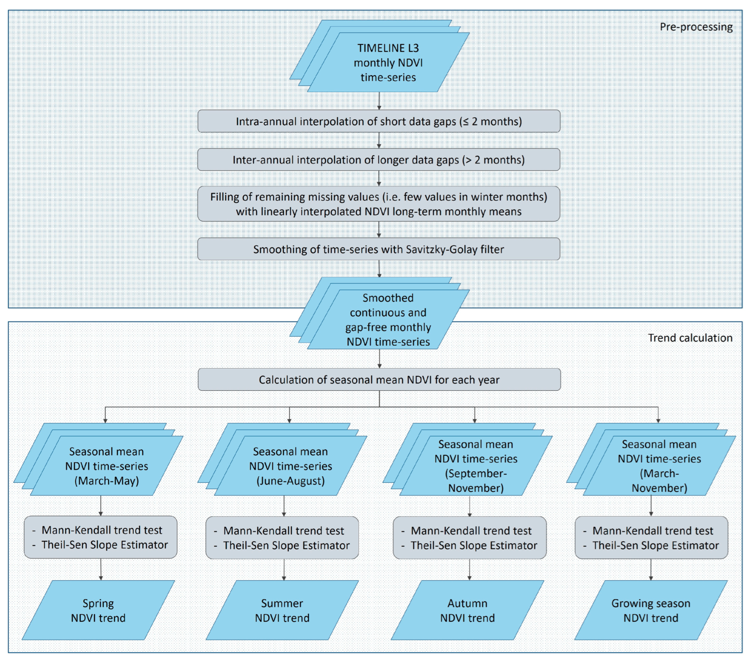
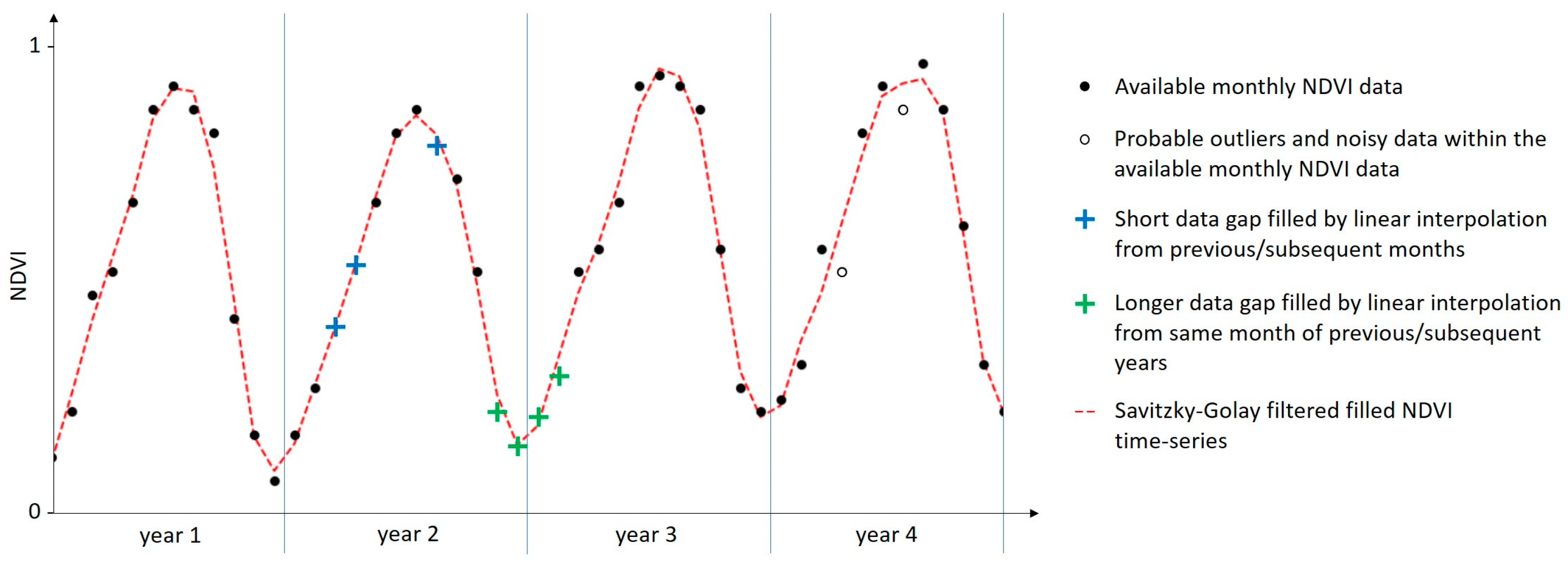
2.4. Pre-Processing of TIMELINE NDVI Time-Series for Trend Analysis

The database used within this study for the seasonal trend analysis comprises the TIMELINE monthly NDVI composites. This time-series includes data gaps (see Section 3.1) that had to be filled to form a continuous time-series for subsequent analyses. A flowchart of the processing steps is presented in Figure 2. Gaps in the time-series were filled and corrected via a four-stage approach (Figure 2 and Figure 3). First, short gaps of one or two subsequent months were filled by linear interpolation of the monthly time-series (intra-annual interpolation). In order to not ignore the phenological cycle, longer data gaps of three or more subsequent months were linearly interpolated from the closest available data of the same month, e.g., from the previous and subsequent year (inter-annual interpolation). Few remaining missing values in winter months were filled by linearly interpolated long-term (1989–2018, i.e., period considered for trend analysis) monthly means in order to retrieve a continuous and gap-free time-series. As a last step, a Savitzky–Golay filter [69] with a filter window of five months in length and a third-order polynomial was applied. Savitzky–Golay filtering is a common method used in remote sensing to smooth vegetation time-series and correct for values influenced by, e.g., clouds [58,70,71]. Figure 3 illustrates the major steps of the procedure applied for filling of data gaps and smoothing of the NDVI time-series within this study.

2.5. Seasonal Trend Analyses

For the analysis of seasonal trends, the seasonal mean NDVI for spring (March to May) summer (June to August) and autumn (September to November) months was calculated from the pre-processed NDVI data for each year. A Mann–Kendall trend test [72,73] was then performed separately for the three seasons to analyse the time-series for consistent positive or negative trends [74]. The Mann–Kendall trend test determines the frequency of the sign of the difference between all pair-wise combinations of data values ($x_j$ − $x_i$, with j > i). This leads to n(n − 1)/2 pair-wise combinations (n = total number of data values). The Mann–Kendall trend test is a non-parametric test, suitable for non-normally distributed data and small sample size [75] that is less sensitive to outliers and uneven distribution compared to parametric tests [76,77]. We consider significant trends to have p-values lower than 0.05. This is a common threshold that represents a statistical significance at the 95% level [53,56,63,65,77,78,79,80,81]. Additionally, we mask areas with more than 50% missing monthly NDVI composite data within the respective season in the period 1989–2018, as well as areas with no or little vegetation cover characterised by a mean annual NDVI of less than 0.2 (compare with Figure 1).

The direction and strength of the trend were calculated using the Theil–Sen Slope Estimator [82,83]. The Theil–Sen Slope Estimator calculates the strength of a monotonous trend as the median of the slopes (${\beta }_i$) of the lines through all point pair combinations ($x_j$and $x_i$ are the data values at times j and i, with j > i):

$${\beta }_i=\frac{x_j-x_i}{j-i} for i=1, \dots , n$$

(2)

The Theil–Sen Slope Estimator is more robust compared to simple linear regression, e.g., ordinary least squares regression, and is resistant to the impact of outliers [84,85]. The usage of the Mann–Kendall trend test in combination with the Theil–Sen slope estimator has efficiently been used for climate-relevant trend analyses in other studies, for example, [38,54,86,87,88].

In addition to the seasonal trends for spring, summer and autumn, a trend for the “growing season”, which was defined to include the months of March through to November, was calculated. In European winter (December–February), vegetation growth is widely hindered due to low temperatures and large parts of the study area being covered by snow. In terms of phenology, the period March to November includes the average beginning and end of the growing season within Europe [89,90].

3. Results

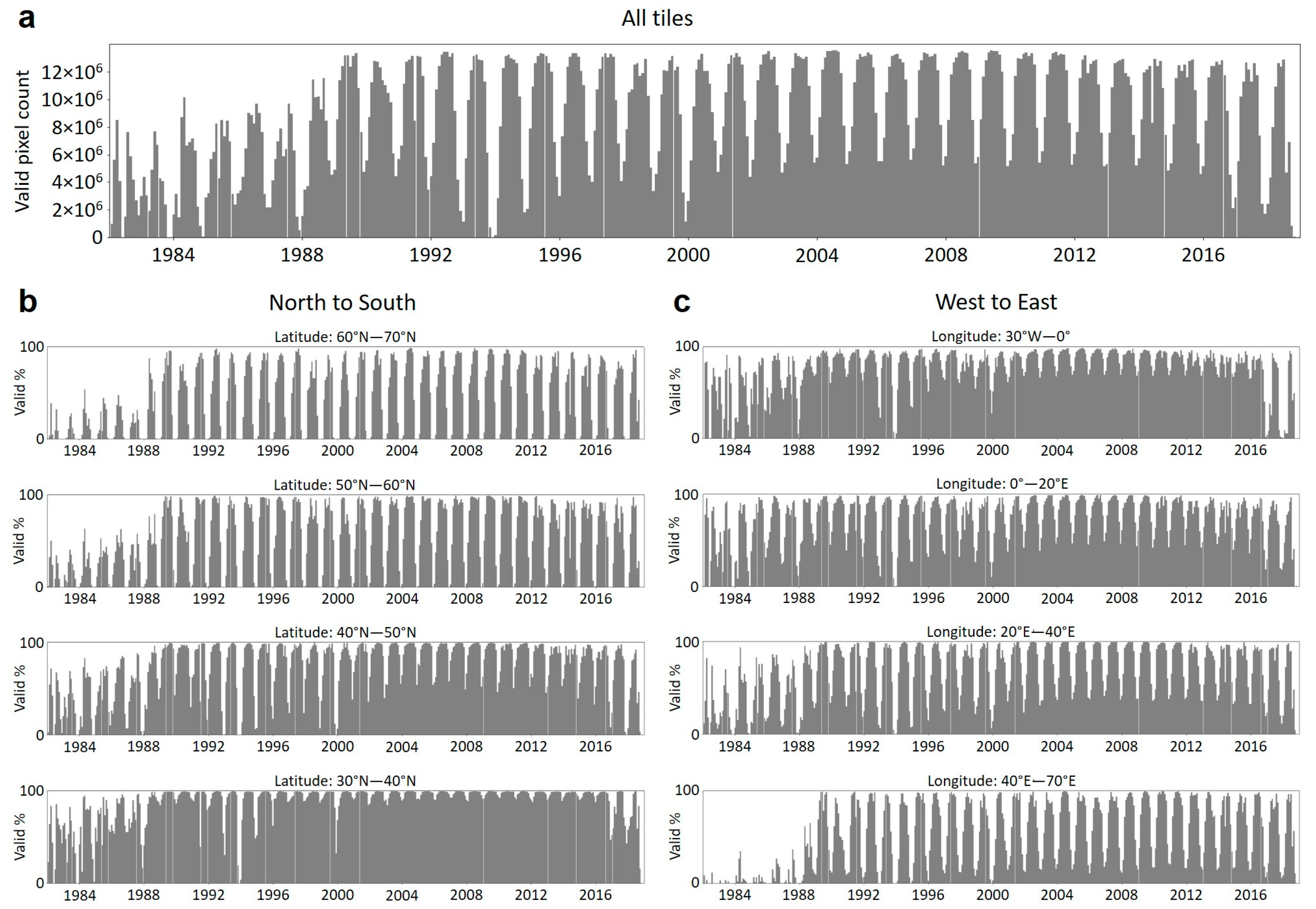
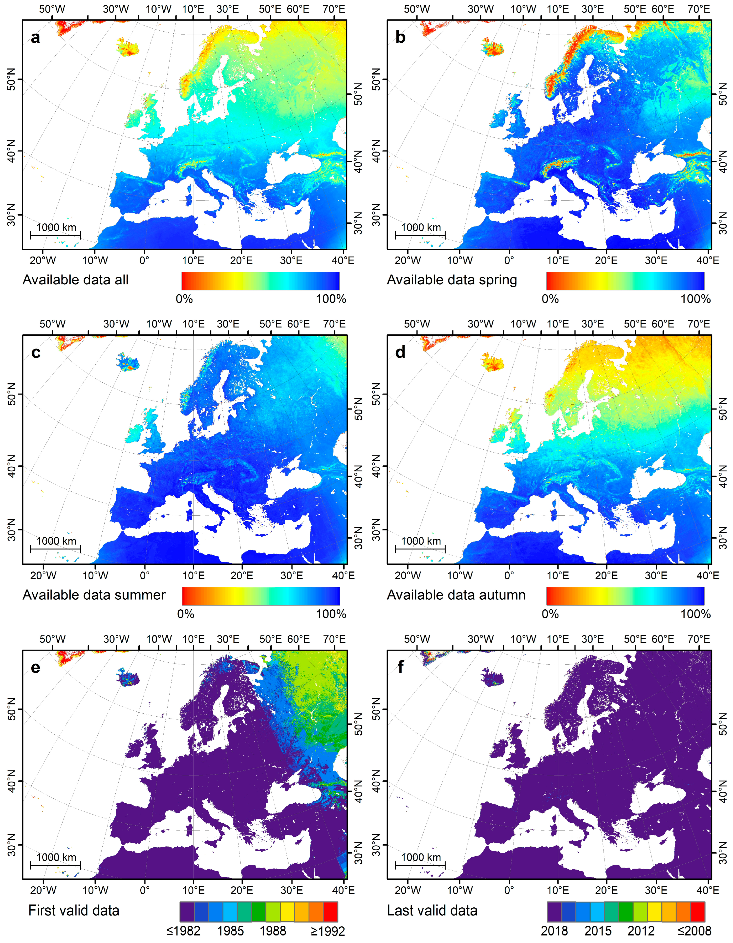
3.1. Spatial and Temporal Availability of TIMELINE Monthly NDVI Time-Series Data

In case of long time-series over large areas, such as the TIMELINE NDVI product, the availability of data within the time-series may vary in space and time. It is important to know the data availability and distribution in order to reliably interpret and analyse the time-series. For the TIMELINE monthly NDVI composite product, we investigated the data availability within the time-series from 1981 to 2018.

The amount of available TIMELINE monthly composite data for 1981–2018 is shown in Figure 4a. Each bar gives the count of valid NDVI pixels over the entire coverage area within the monthly NDVI composites. Figure 4b,c present the percent of valid NDVI pixels in the defined latitude (30°–40°N, 40°–50°N, 50°–60°N and 60°–70°N) and longitude (30°W–0°, 0°–20°E, 20°–40°E and 40°–70°E) ranges. It can be observed that overall, fewer data are available in the beginning of the time-series for the years 1981 to 1988. A clear seasonal pattern can be observed especially for northern latitudes with missing NDVI data in winter due to large sun zenith angles and snow coverage. In the eastern part of the coverage area, only a few NDVI data are available within the first eight years of the time-series. Data availability is generally higher towards the south and west of the study area. The increasing seasonality towards the east can be explained by extensive snow coverage due to the continental climate, the landmass distribution with more land in higher latitudes in eastern Europe compared to western Europe, and the coverage area of the TIMELINE products that extends furthest to the east at about 59°N (compare with Figure 1).

Figure 5a shows the availability of monthly NDVI composite data per pixel as the percentage of the maximum possible count of data for the period 1981–2018 (i.e., 100% represents a count of 446 composites). A clear gradient from the north (few data) to the South (many data) as well as from mountainous areas (few data) to lower-lying areas (many data) can be observed. The data availability is also reduced for the Canary Islands and the Azores. For Greenland, almost no NDVI data are available. The period October 1981 to November 2018 comprises 446 months. The maximum number of available monthly composite data counted on a per-pixel basis is 434. This indicates that at least a few time-series data are missing for every pixel within the study area.

Additionally, the percentages of available monthly NDVI data for the three seasons of spring (March–May), summer (June–August) and autumn (September–November) were separately examined. This provides important information for the seasonal analyses. The distribution of available data for the three seasons are shown in Figure 5b–d. For better comparability, the time period considered for the count of seasonal data was restricted to the years 1982 to 2018. The maximum possible count of monthly data per season for these 37 years is 111, represented by 100%. The figure for spring (Figure 5b) shows the lowest data availability for mountainous regions. A reduction in available data can also be located at high latitudes, in Iceland and continental eastern Europe. For summer (Figure 5c), data availability is generally good with fewer data in eastern (>60°E) Europe, parts of Iceland, Ireland, Scotland as well as high mountainous regions. The availability of data for autumn (Figure 5d) shows a pronounced gradient from north to south with fewer data for more northern regions and an influence of terrain height with fewer data for mountainous areas.

For investigations that consider the timely development of NDVI over several years, the availability of NDVI data within different years is also important. The number of AVHRR observations varies between years and is considerably lower in earlier years [29]. Thus, for the early 1980s, fewer scenes were available for NDVI composite generation. In order to further investigate this aspect, the month of the first available NDVI data was recorded for each spatial location. Figure 5e shows the corresponding year in which the first NDVI monthly composite data are available. For most of Europe, the first data are available in 1981 or 1982 (dark purple). In the eastern part with longitudes > 35°E, the first data are present later, e.g., in 1984 (blue), 1986 (mint green) and 1988 (light green). Analogously, Figure 5f shows the corresponding year representing the month of the last available data within the current TIMELINE L3 NDVI product time-series. Except for Greenland and a glacier area in Iceland, no larger regions within Europe are affected by constantly missing NDVI data at the end of the NDVI time-series.

For trend analyses, it is important to have valid data for the entire time period considered. The data availability analysis reveals that a large area in the northeast of the TIMELINE study region is characterised by missing data within the first eight years (Figure 4 and Figure 5e). Considering this observation, the time period for the subsequent NDVI trend analysis of this study was confined to the years 1989–2018 to be able to include the entire TIMELINE study area.

3.2. Seasonal NDVI Trends for Spring, Summer, Autumn and the Growing Season (1989–2018)

The results of the trend analyses for the years 1989–2018 are presented in the following figures separately for spring (Figure 6 and Figure 7), summer (Figure 8 and Figure 9) and autumn (Figure 10). Figure 11 shows the trend for the growing season including the period from March through to November, as described in Section 2.5. The figures cover the extent of the TIMELINE L3 NDVI product (compare with Figure 1). In the presented main figures of the seasonal trends (Figure 6a, Figure 8a, Figure 10a and Figure 11a), only significant trends are shown. Trends with a significance level of p ≥ 0.05 were considered insignificant. In addition, for all main figures, areas with less than 50% of possibly available monthly NDVI composite data present within the respective season in the period 1989–2018 were masked. Moreover, areas with little or no vegetation cover characterised by a mean annual NDVI of less than 0.2 were also masked. The side-figures on the right within Figure 6, Figure 8, Figure 10 and Figure 11 present the unmasked slope of the regression from the Theil–Sen Slope Estimator (b) and the p-value of the Mann–Kendall trend test (c) for each of the seasonal trend analyses.

Additionally, two tables are provided that give numerical information about the four seasonal trends derived.

Table 2. Area with negative or positive NDVI trends with p < 0.05 (significant) or p ≥ 0.05 (insignificant), respectively, as well as masked land area (mean annual NDVI < 0.2 or available monthly NDVI data < 50%), given as percentage of total land area within the extent of the TIMELINE L3 NDVI product [%], and absolute area [km²] for different seasons.

	Negative (p < 0.05)		Negative (p ≥ 0.05)		Positive (p < 0.05)		Positive (p ≥ 0.05)		Masked Land Area
	[%]	[km2]	[%]	[km2]	[%]	[km2]	[%]	[km2]	[%]	[km2]
Spring	3.61	496,748	16.58	2,281,464	20.89	2,874,535	38.01	5,230,305	20.91	2,877,287
Summer	6.20	853,141	20.12	2,768,580	21.58	2,969,481	35.87	4,935,834	16.23	2,233,303
Autumn	4.55	626,095	10.71	1,473,732	25.28	3,478,614	19.03	2,618,593	40.43	5,563,305
Growing season	2.17	298,599	7.99	1,099,451	55.43	7,627,356	18.44	2,537,407	15.97	2,197,526

presents the area that experienced significant or insignificant negative or positive trends for each season. Each area is given as the percentage of the total land area (13,760,339 km²) within the extent of the TIMELINE L3 NDVI product, and as the absolute area.

Table 3. Average strength of trends observed for negative and positive NDVI trends with p < 0.05 (significant) and p ≥ 0.05 (insignificant), respectively, for the different seasons. The strength of the trends is expressed in NDVI units over the 30-year study period (1989–2018).

	Negative (p < 0.05)	Negative (p ≥ 0.05)	Positive (p < 0.05)	Positive (p ≥ 0.05)
Spring	−0.1114	−0.0320	0.1202	0.0455
Summer	−0.0992	−0.0281	0.0918	0.0319
Autumn	−0.1222	−0.0346	0.1369	0.0436
Growing season	−0.1198	−0.0340	0.1483	0.0457

gives the average strength of the trend within areas of significant or insignificant negative or positive trends, expressed in NDVI units over the 30-year study period (1989–2018). The columns with p < 0.05 (significant trend) correspond to the negative and positive trends shown in the main figures (a) within Figure 6, Figure 8, Figure 10 and Figure 11.

The NDVI trend for spring (Figure 6) shows some areas with negative or positive trends that are distributed over the study area and covering a local to regional extent. The total area experiencing a significant positive trend sums up to 2,874,535 km², which corresponds to 20.89% of the land area within the extent of the TIMELINE project area (Table 2). The average NDVI increase within the area with significant positive spring NDVI trends (blue area in Figure 6a) is 0.12 NDVI units over the 30-year period 1989–2018 (Table 3). Larger areas with positive trends can be observed in central Europe, including eastern Germany and Czechia, in south-eastern Europe, with the strongest positive NDVI trends located in southern Romania, along the southern coast of the Black Sea, as well as for a larger area in north-eastern Europe starting from Sweden and spreading over Finland and Russia (Figure 6). Moreover, positive spring NDVI trends can be observed within other smaller regions for example in Italy, France, Great Britain, parts of Spain, or Algeria.

The area for which significant negative spring NDVI trends are observed extends over 3.6% of the study area, covering 496,748 km² (Table 2). Its average trend is −0.11 NDVI units over the 30-year study period (Table 3). Negative spring NDVI trends can be observed, for example, for Morocco, parts of the Canary Islands, parts of Spain and within the Landes forest in France (Figure 6). The continental part of eastern Europe also shows negative trends for the central Ukraine and on both sides of the Volga river in Russia. Moreover, in parts of Tunisia, Libya, the Nile Delta in Egypt, and Israel, negative spring NDVI trends can be found.

The spatial resolution of the TIMELINE NDVI product of 1 km also allows us to capture NDVI trends on a local scale. Three examples of locally outstanding spring NDVI trends are shown in more spatial detail in Figure 7. Having a look at these areas at higher resolution and comparing satellite imagery of the same areas from the years 1989/1990 and 2018, it becomes apparent that the trends observed in these areas can be explained by land management and land-use change. For example, in northern Russia, defined areas with a negative spring NDVI trend can be observed that can be attributed to forest logging (Figure 7A). Another example of local man-made changes is the areas with increasing irrigated agriculture that show spatially limited positive spring NDVI trends, and this can be found, for example, on both sides of the Nile Delta (Figure 7B). The core area of the Nile Delta, in contrast, shows a negative NDVI trend, which can be explained by urban expansion encroaching on established agricultural lands [91,92,93]. The third example within Figure 7 shows an area with several newly established agricultural fields in Saudi Arabia (Figure 7C) that are characterised by a strong NDVI increase within the period 1989–2018.

The summer NDVI for 1989–2018 (Figure 8) shows comparatively low trends distributed over Europe in a rather patchy pattern. The average strength of the significant positive trends is 0.09 NDVI units, and that of the negative trends is −0.10 NDVI units over the 30-year period of investigation (Table 3). The trends that can be observed for central, northern and south-eastern Europe are mainly positive, but patches with a negative trend can also be located on a small scale all over the area (Figure 8). England shows partly positive trends, while the summer NDVI trend in Scotland and Ireland is rather negative. Spain also shows distinct areas with positive or negative trends. Positive trends dominate in the north, while large parts of the country experience negative summer NDVI trends. Larger areas dominated by significant negative summer NDVI trends can be found in Morocco, southern Russia and West Kazakhstan. Turkey also shows some areas with significant negative trends, but the western part of the country experiences mainly positive trends (Figure 8).

Though about 26% of the land area investigated experiences negative summer NDVI trends, for only 6.2% of the area (853,141 km²), this trend is significant at the 95% level (Table 2). The area with significant positive summer NDVI trends extends over 21.6% of the study area.

The summer NDVI also features some areas with outstanding NDVI trends. Three selected areas are presented in Figure 9 at a higher spatial resolution to allow for identifying patterns within these areas. The first detail view shows a surface mining area in eastern Germany (Figure 9D). Three small defined sites with negative NDVI trend stand out that coincide with areas of surface mining (open-cast mines Nochten, Welzow and Jaenschwalde). Former surface mines, which have been recultivated within the period of investigation, can be identified by a strong NDVI increase (Figure 9D). The other two example areas include agricultural fields that have been established or intensified during the period of investigation. These agricultural fields can be identified based on their strong positive summer NDVI trend, for example, in the area in north-eastern Spain (Figure 9E). The example area shown in Figure 9F can be found in Şanlıurfa/Mardin provinces in southern Turkey and also features outstanding positive NDVI trends that can be associated with agricultural development in this area.

The autumn NDVI trend for 1989–2018 (Figure 10a) shows a significant positive trend for large parts of western, central and south-eastern Europe. Eastern Europe also has a positive trend except for a larger region around the Sea of Azov, for which a negative trend can be observed. In northern Europe, areas in high latitudes have been masked due to low data availability, and thus, no trend is shown.

Parts of Morocco are characterised by a negative NDVI trend for autumn during the period 1989–2018, while the observed trend in northern Algeria and Tunisia is rather positive. Spain and Turkey show patches of both positive and negative trends. Some agricultural areas established during the period of investigation can again be clearly identified as locally limited areas with a high positive autumn NDVI trend.

The area with significant positive autumn trends comprises 3,478,614 km² (25.3% of the land area) and shows an average increase of 0.14 NDVI units over the 30-year period of investigation. The area with significant negative trends covers 626,095 km² (4.6%) with an average decrease of −0.12 NDVI units over the 30-year study period (Table 2 and Table 3).

The NDVI trend for the growing season shows a positive trend for most of Europe (Figure 11). More than 55% of the land area covered by the TIMELINE NDVI product has a significant positive trend (7,627,356 km²) with an average strength of 0.15 NDVI units over the period of investigation (Table 2 and Table 3). The growing season NDVI trend is significant at a level of even p < 0.01 for large parts of the study area (Figure 11c). The regions experiencing strongest positive growing season NDVI trends can be located in central and south-eastern Europe, but also, northern, western, southern and eastern Europe show mostly positive NDVI trends. Agricultural areas established during the period of investigation, e.g., in Turkey, Egypt and Saudi Arabia, stand out as locally limited areas with a high positive NDVI trend.

Some areas with a negative NDVI trend for the growing season can also be identified. These areas, however, comprise only a small part of the study area (2.2%, i.e., 298,599 km²; Table 2). Strong negative trends are observed for parts of the Canary Islands (this might also be influenced by low data availability; see Section 4.3) and parts of Morocco. Small areas in central and southern Spain, as well as areas in Libya, the Nile delta, Israel and Turkey, also show a negative NDVI trend when considering the entire growing season. For the area around the Sea of Azov, covering parts of south-eastern Ukraine, southern Russia and West Kazakhstan, negative NDVI trends for the growing season can also be observed during the period 1989–2018.

4. Discussion

4.1. Data Availability within the TIMELINE L3 Monthly NDVI Product

In this study, we present the TIMELINE NDVI product and investigate the data availability of the monthly NDVI composites and how it varies temporally and spatially. The results with respect to data availability within the monthly NDVI time-series show a seasonal pattern with data gaps during the winter season that are especially pronounced in the north of the study area. This can be explained by less data availability towards northern latitudes due to lower sun illumination and the larger snow coverage in winter, which lead to a reduced number of valid observations. In mountainous regions, the NDVI data availability is also reduced due to longer snow coverage. Therefore, NDVI analyses for the winter period and snow-covered areas are limited.

A reduced data availability can also be observed in the beginning of the time-series. Especially in the eastern part (east of ca. 35°E) of the product coverage area, NDVI data are missing for the first years. The time period to be included for possible future data analyses for this area should be adjusted accordingly, similarly to the adjustment made in this study. The data availability is also reduced for the Canary Islands and is very limited for the Azores and Greenland. The data for the years 1981 to 1988 should generally be handled with caution, because a lower number of AVHRR observations are available for NDVI composite generation during this period before the start of NOAA-11 [29,41].

In this study, to be able to cover the entire TIMELINE area, the time period for the trend analysis was limited to 1989–2018. Due to the long time coverage of the TIMELINE product, this still leaves 30 years for the trend analysis, which can be considered sufficient to allow climate-relevant statements to be made [28,29].

4.2. Generation of Continuous NDVI Time-Series

The TIMELINE monthly composite NDVI time-series includes data gaps due to different reasons including snow and cloud coverage, periods of low sun zenith angles, or missing observations. In this study, we therefore implemented an approach for gap-filling and smoothing of the NDVI time-series on a per-pixel basis in order to generate a continuous NDVI time-series suitable for subsequent analysis. Our approach combines “intra-year” interpolation for short gaps of up to two months with “inter-year” interpolation for longer time periods. This approach was chosen in order to also maintain the phenological cycle in case of longer data gaps. An advantage of our approach is that it relies only on the available data of the TIMELINE L3 NDVI product. In contrast to filling with other products, this is more straightforward and avoids integrating errors or inconsistencies due to differences in spatial resolution, geometry and calibration. A Savitzky–Golay filter was finally applied in order to remove outliers and to smooth the time-series.

The filling of missing data is an important step required for time-series analyses. In comparison to other NDVI studies, for which solely linear interpolation has been applied, e.g., using Satellite Pour l’Observation de la Terre—Végétation (SPOT-VGT), GIMMS or MODIS NDVI data [49,70,94,95], we suggest using a method that is also able to keep the NDVI phenological signal in case of requiring the reconstruction of longer data gaps for the TIMELINE NDVI time-series. There are several possible pre-processing methods, and the choice of which to use depends upon the subject of the envisaged analysis and the study region, for example [54,96,97,98,99,100,101].

4.3. Discussion and Comparison of NDVI Trends

In this study, we present seasonal trends for the 30-year period from 1989 to 2018. The distribution and strength of the observed trends differ among spring, summer and autumn seasons. Having a look at the growing season, we observe a mainly positive NDVI trend for Europe with some regional exceptions (compare with Figure 11). The trends for individual seasons show distinct patterns and reveal vegetation dynamics occurring only for specific seasons. Especially in summer, the NDVI trend does not show a European-wide greening, but it shows negative NDVI trends for several regions (compare with Figure 8). Positive trends in summer are regionally limited and less pronounced compared to the growing season trend. In spring, the NDVI trend also shows a patchy distribution with both positive and negative trends, while in autumn, positive trends extend over a rather large area. For some regions, significant trends can be identified for only one season (e.g., positive trend in spring for the region along the lower reach of the Danube River), while other regions are characterised by varying or opposing trends in different seasons (e.g., the region north of the Caucasus mountains between the Black Sea and Caspian Sea; several areas within the Iberian Peninsula). The seasonal trends reveal that the development of vegetation condition is not constant throughout the growing season. The results show that the individual trends for spring, summer and autumn provide additional information compared to the growing season trend.

Comparisons to previous studies on NDVI trends can mainly be performed for the growing season, as individual seasons have rarely been analysed [38,52]. It has to be considered that other studies often include a shorter or differing time period and are partly based on other variables, mostly the annual mean NDVI. Most previous NDVI trend analyses have been performed on a global scale with a low spatial resolution. Few studies include smaller regions within Europe or focus on specific land cover classes, such as [38,86]. None of the previous studies presented NDVI trends for three decades for the whole of Europe with a 1 km spatial resolution.

The comparison of our results with other studies shows that the distribution of areas with a positive/negative trend corresponds to the results of previous research. An early study from Xiao and Moody [52] analysed NDVI trends globally for 1982–1998 using the AVHRR-derived Pathfinder NDVI dataset and found a positive annual NDVI trend for most of Europe ranging between 1% and 14%. The strongest positive trends are observed for central and eastern Europe, the UK and southern Sweden. For the south of Spain, a negative NDVI trend was found. Seasonal trends were less pronounced with mainly positive trends. Julien et al. [50] presented the NDVI difference between the periods 1982/1986 and 1995/1999 derived from the Pathfinder AVHRR Land dataset. They reported an NDVI decrease in arid and semiarid areas (northern Africa, southern Spain, Middle East) and an increase in temperate areas (western and central Europe) with a stronger increase in NDVI mean values, especially for Germany, Czech Republic, Poland and Belarus, where NDVI values have increased by more than 0.07. Beck et al. [53] compared annual mean NDVI trends from four AVHRR-based Global Area Coverage NDVI datasets for the period 1982–1999. The trends observed for Europe differ in magnitude among datasets, but they predominantly show a “greening” of vegetation for Europe. The spatial distribution of trends from these early studies [50,52,53], in general, fit to the trends observed in our study, though it has to be considered that they only overlap by about 10 years with our study.

De Jong et al. [54] retrieved NDVI trends for the period 1981–2006 based on GIMMS NDVI. The trend within Europe was negative for southern Spain/Portugal, while the rest of Europe showed mainly positive or insignificant trends. The areas showing strongest positive trends coincide with those observed in our study. Sobrino and Julien [55] also observed a positive trend of yearly integrated GIMMS NDVI over Europe similarly to other studies. They also report an increase in growing season length for central, eastern and northern Europe. Fensholt and Proud [56] analysed GIMMS and MODIS NDVI for the ten-year period between 2000 and 2010. Large areas in Europe showed no significant trend. The linear trend based on monthly observations was negative, e.g., for parts of Spain, Portugal and France. The strongest negative trends were observed within southern Russia and western Kazakhstan, where, in this study, a negative summer NDVI trend was found as well. Positive trends were reported, e.g., for the eastern coast of Spain, southern Europe, Turkey and Algeria. The trends are presented in the range +/−0.1 over the study period and show lower values for GIMMS compared to MODIS NDVI. Eastman et al. [61] also report an increase in mean NDVI for the period 1982–2011 for large areas within Europe and an increase in the difference between minimum and maximum NDVI without affecting the mean for continental eastern Europe. The areas of increasing NDVI coincide with positive NDVI trends in our study. Liu et al. [57] present the annual rate of change in NDVI for the period 1982–2012 based on GIMMS NDVI. They report a greening for large areas in Europe and insignificant or partly negative trends for the area north of the Black Sea towards the Caspian Sea, findings which are consistent with our results. The strength of the presented trend is also in a comparable range to our results. Wang et al. [58] compared global VI trends for the period 2001–2016. The GIMMS NDVI trend was positive for most of Europe and negative for northern areas such as Norway, areas within the Iberian Peninsula, and central and eastern Europe. Pronounced negative vegetation trends were observed for the southern part of eastern Europe (Ukraine, southern Russia, Kazakhstan), coinciding with the trends observed in our study. Zhang et al. [59] present global annual NDVI trends for the period 2001–2015 based on MODIS Terra NDVI that also show mainly positive trends except for the area covering the south of the Ukraine towards Kazakhstan, where positive trends are observed. For the period 1981 to 2015, He et al. [51] reported an increasing NDVI for large parts of Europe based on GIMMS data, but also no or negative trends in the Ukraine/Russia/Kazakhstan area, where we observe negative NDVI trends. Their results are in good agreement with our observations.

For the central-eastern part of the study area, covering parts of the Ukraine, southern Russia and Kazakhstan, where we observe negative NDVI trends, other previous studies have also reported negative NDVI trends, especially those including more recent years [51,56,58,59]. In the area with a decreasing summer or autumn NDVI trend, a decreasing trend in summer precipitation between 1960 and 2015 was also reported by the European Environment Agency (EEA) [102]. Stöckli and Vidale [103] found a trend towards an earlier occurrence of autumn phases based on a 20-year AVHRR dataset from 1982 to 2001 for most of the areas with a negative autumn NDVI trend in the Ukraine/Russia/Kazakhstan region from our study. A comparison of the trends in this region with a land cover map (ESA CCI [104]) reveals that negative trends are mostly located in agricultural areas, while forests show mainly positive trends for the growing season and insignificant or positive trends for summer and autumn. A recent publication by Yao et al. [105] found that water reservoirs in this area experience the strongest negative water storage trend for the period 1992–2020 within Europe. Lake volume loss in that region could be attributed to temperature and potential evapotranspiration or precipitation and runoff [105].

A more spatially detailed comparison of NDVI trends is possible with regional studies, such as the study by Vicente-Serrano et al. [38], who analysed NDVI trends in Spain for the period 1981–2014 with a 1.1 km spatial resolution and also presented results for individual seasons. The areas showing negative or positive trends are in generally good agreement with the results of our study for all seasons. The magnitude of change is also in a similar range for both studies. Our results are also generally consistent with previous studies for Spain considering previous and shorter time periods [106,107].

Prâvâlie et al. [86] analysed the summer season (June–August) NDVI for forest areas in Romania and reported a countrywide increase in NDVI during the period 1987–2018. Only a small part of the forest area showed a decreasing trend, which is also partly present in our results but has been masked as insignificant.

For Tenerife and Gran Canaria, for which we observe partly strong negative NDVI trends, no regional NDVI trend analyses were found for comparison. Global studies have too coarse a resolution to be able to identify trends for this area. However, climate trends with increasing temperatures have been reported for the Canary Islands [108,109], which might have caused negative vegetation trends. The mean yearly temperature for the Canary Islands shows an increase of 0.7 °C for the period from 1979 to 2021, while the precipitation trend shows a decrease from 251 mm to 217 mm [110]. However, the trend observed for the Canary Islands might also be affected by lower data availability due to their location at the edge of the observation area (most south-western area) with fewer data available especially at the beginning of the time-series. Exceptionally high NDVI values within the first years might have affected the derived trend.

For the Alps, a previous study by Choler et al. [78] observed a greening trend for the 2000–2020 period. Asam et al. [111] detected an overall increasing NDVI for 2000–2017 based on MODIS over the Alps. In our study, a greening can also be observed for the Alps region when looking at the autumn and growing season trends. Some individual pixels and small areas with a negative NDVI trend are present in our results, which are located in areas with a data availability just above 50% in the NDVI time-series. Thus, the negative trend for these pixels might be caused by the low number of original NDVI observations. Applying a higher percentage for the mask (e.g., two-thirds of valid composite data are required within the time-series) would mask these areas.

A regional NDVI trend study is also available for Iceland. Raynolds et al. [112] analysed the AVHRR (GIMMS with 12.4 km resolution)-derived NDVI trends of Iceland from 1982–2010, as well as MODIS NDVI for the period 2002–2013. The GIMMS trend is mostly positive until the year 2000, but from then, negative NDVI trends are more common until 2010. The negative trend was confirmed with the MODIS dataset. The results for the summer NDVI trend from this study are in good agreement with the MODIS maximum annual NDVI trend presented by [112], showing similar spatial distribution and magnitude of trends.

Our results for northern Africa can be compared to a study by Barrio et al. [113], who observed a similar pattern with respect to land condition trends for the period 1998–2008. Their results generally confirm the trends observed for the growing season NDVI in our study for Morocco, Algeria and Tunisia.

The comparison shows that the NDVI trends observed in this study are generally consistent with previous studies. Our findings confirm the greening trend that has been reported for large parts of Europe, and due to the longer time-series as well to the higher spatial resolution, reinforce this finding with a higher reliability. On a regional scale and for individual seasons, the NDVI trends of this study show detailed and spatially explicit trends with variations in positive and negative trends, which agree with regional research and add details of the development of vegetation condition.

4.4. Comparison of TIMELINE L3 NDVI and Other AVHRR NDVI Products

The TIMELINE L3 NDVI product is a novel product complementing other available NDVI products derived from AVHRR data. Table 4 gives on overview of the TIMELINE L3 NDVI product features in comparison to examples of other currently available AVHRR NDVI products of at least national or continental coverage. Table 4 provides information about spatial coverage and resolution, temporal coverage and resolution, and the data provider for each product.

The majority of AVHRR NDVI products listed in the table are available on a global scale. One product is available for Canada, and one product is available for Peninsula Spain and the Balearic Islands. The resolution of the grid cells varies from 1 km to 16 km and 0.05 degrees to 0.5 degrees. The NDVI products are available on a monthly basis up to daily intervals. Currently, only NOAA and NASA produce global data products which cover the full time-series from the 1980s up to the present day. These long-term time-series are available at a spatial resolution of 0.05 degrees or 4 km grid size only. NDVI products with a 1 km spatial resolution are available on a national scale or produced for a certain limited time period. In this context, the widely used MODIS NDVI products should also be mentioned. The MODIS Vegetation Index Products provide NDVI time-series at different spatial (0.25 km, 0.5 km, 1 km, 0.05 degree) and temporal (16-day, monthly) resolutions [114]. However, the MODIS NDVI products are only available over the MODIS time span from 2000 onwards. Currently, no NDVI product over Europe exists covering the full time-series of four decades and offering a spatial resolution of 1 km. This gap is filled by the TIMELINE NDVI product.

Table 4. Parameters of the TIMELINE L3 NDVI product and examples of other currently available AVHRR NDVI products.

Product	Spatial Coverage	Temporal Coverage	Spatial Resolution	Temporal Resolution	Produced by
TIMELINE L3 NDVI	Europe and northern Africa	1981–2018 (will be continued)	1 km	daily, 10 days, monthly	DLR
LTDR NDVI [115]	Global	1981–present	0.05 degree	daily	NASA
NOAA CDR of AVHRR NDVI V5 [35]	Global	1981–present	0.05 degree	daily	NOAA
Boston University NDVI [116]	Global	1981–2001	16 km, 0.5 degree	monthly	Boston University
NDVI3g GIMMS [30,31]	Global	1981–2015	1/12 degree	15 days	NASA/GFSC
NDVI V2 (ENDVI10) [34]	Global	2007–present	1 km	10 days	VITO/EUMETSAT LSA SAF
Crop Condition Assessment Program (CCAP) NDVI [36]	Canada	1987–2020	1 km	daily, weekly	Statistics Canada
Sp_1 km_NDVI [38]	Spain	1981–2015	1 km	semi-monthly	Spanish National Research Council

Table 4. Parameters of the TIMELINE L3 NDVI product and examples of other currently available AVHRR NDVI products.

Product	Spatial Coverage	Temporal Coverage	Spatial Resolution	Temporal Resolution	Produced by
TIMELINE L3 NDVI	Europe and northern Africa	1981–2018 (will be continued)	1 km	daily, 10 days, monthly	DLR
LTDR NDVI [115]	Global	1981–present	0.05 degree	daily	NASA
NOAA CDR of AVHRR NDVI V5 [35]	Global	1981–present	0.05 degree	daily	NOAA
Boston University NDVI [116]	Global	1981–2001	16 km, 0.5 degree	monthly	Boston University
NDVI3g GIMMS [30,31]	Global	1981–2015	1/12 degree	15 days	NASA/GFSC
NDVI V2 (ENDVI10) [34]	Global	2007–present	1 km	10 days	VITO/EUMETSAT LSA SAF
Crop Condition Assessment Program (CCAP) NDVI [36]	Canada	1987–2020	1 km	daily, weekly	Statistics Canada
Sp_1 km_NDVI [38]	Spain	1981–2015	1 km	semi-monthly	Spanish National Research Council

4.5. Outlook and Further Development of TIMELINE L3 NDVI Product

In this study, NDVI trends for the period 1989–2018 for Europe were investigated. Within further studies, additional analyses can be conducted based on the TIMELINE NDVI product within various thematic contexts. The time coverage of almost 40 years and spatial resolution of 1 km allow for long-term analyses to be performed on a pan-European to regional scale. Moreover, the high temporal resolution of the 10-day or daily NDVI products may additionally be used for analyses with respect to phenological patterns such as the start and end of the growing season.

The TIMELINE NDVI product is also subject to further development. Data processing for the extension of the time-series to more recent years including additional NOAA and Meteorological Operational Satellite (MetOp) AVHRR data is currently ongoing.

5. Conclusions

We present the TIMELINE NDVI product, which provides a novel set of daily, 10-day and monthly NDVI composites derived from AVHRR data for Europe and North Africa. The NDVI composites have a spatial resolution of 1 km and currently span the period 1981–2018. The total number of generated datasets currently comprise 42,067 daily composites (~300 GB), 4762 10-day composites (~89 GB) and 1683 monthly composites (38.5 GB).

In this study, we analysed the temporal and spatial data availability within the monthly TIMELINE NDVI time-series. Both seasonal and geographic differences and areas with lower data availability in the beginning of the time-series are identified and presented. A clear seasonal pattern can be observed with missing NDVI data in winter, especially for northern latitudes. Overall, fewer data are available at the beginning of the time-series for the years 1981 to 1988. For this period, fewer AVHRR scenes were available for composite generation. While for most of the study area, the first data are available in 1981 or 1982, the most eastern part of the study area with longitudes > 35°E is affected by missing data for up to eight years at the beginning of the time-series. Other regions at the border of the study area, such as Greenland, the Azores and Canary Islands, are also affected by missing data in the 1980s. The presented results of the data availability analysis are important to understand the possibilities and limitations of the TIMELINE NDVI product for time-series analyses.

Additionally, we derived and investigated seasonal and growing season NDVI trends for the period 1989–2018 based on the TIMELINE NDVI product. Our analysis covers the entire TIMELINE project area. Areas with a mean annual NDVI < 0.2 or a data availability of monthly composites < 50% for the respective season were masked. The following findings with respect to area coverage and strength of the trends for spring, summer and autumn can be concluded:

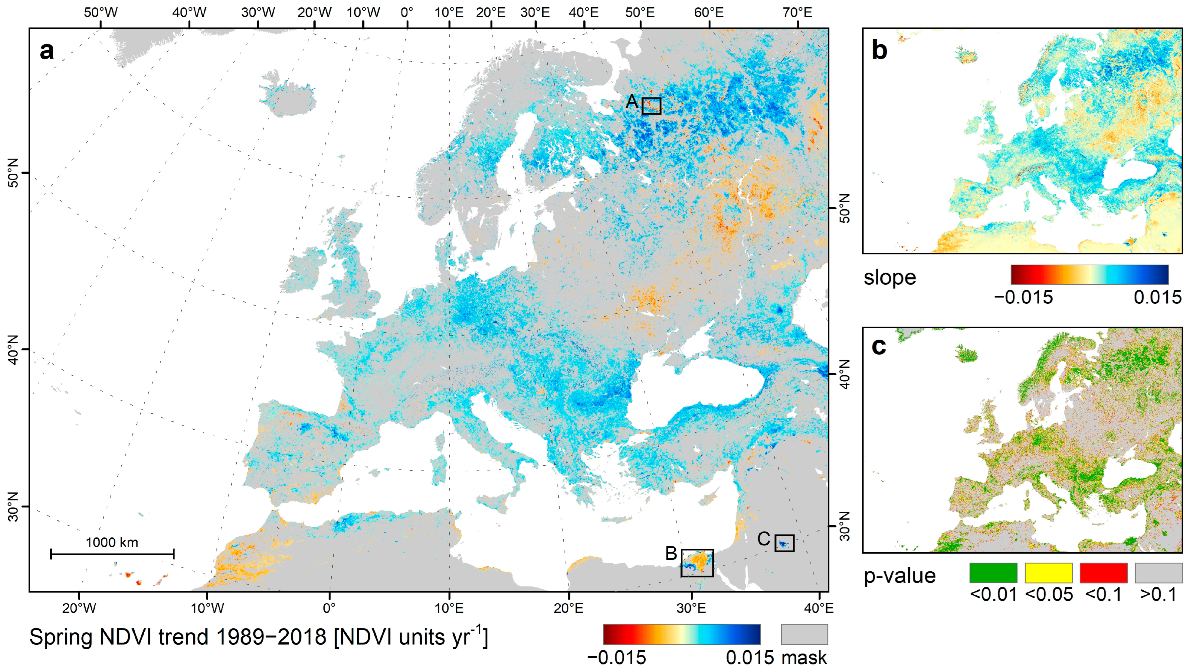
• In spring, an area of 2,874,535 km² (20.9% of the land area within the TIMELINE project area) shows a significant (p < 0.05) positive NDVI trend, while 496,748 km² (3.6%) has a significant negative trend.
• The area with negative NDVI trends is largest for summer, with 853.141 km² (6.2%) experiencing a significant negative trend. Including both significant and insignificant trends, a total area of 3,621,721 km² (26.3%) is affected by negative trends in summer. Significant positive trends are observed in summer for 2,969,481 km² (21.6% of the land area).
• In autumn, the areas affected by significant positive and negative trends cover 3,478,614 km² (25.3%) and 626,095 km² (4.6%), respectively. About 40% of the land area was masked due to low mean annual NDVI or low data availability in autumn.
• The average strength of the significant (p < 0.05) trends varies between spring, summer and autumn. The strongest average trends can be observed in autumn, with −0.12 NDVI units over the 30-year period 1989–2018 for negative trends and 0.14 NDVI units for positive trends. In summer, the average strength over all areas with significant trends is weakest, with about −0.1 NDVI units for negative trends and 0.09 NDVI units for positive trends, again, both given over the 30-year period 1989–2018.

The trends for individual seasons (spring, summer, autumn) show distinct spatial distributions of positive and negative trends. For selected geographical regions, the following larger patterns and observations can be summarised:

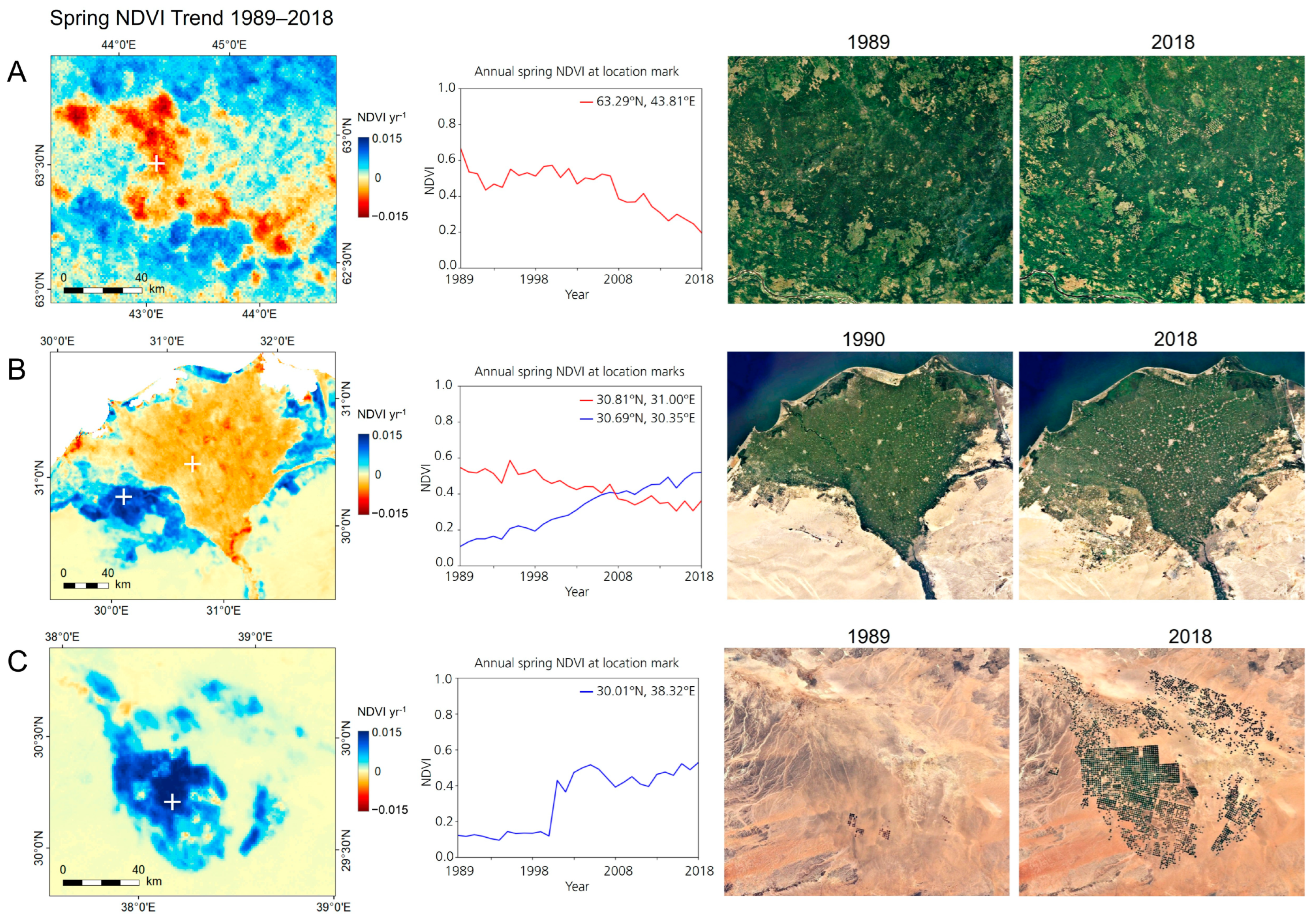
• Scandinavia: Positive spring NDVI trends can be observed within a strip spreading from Norway over central Sweden to southern Finland. In summer, the region has mostly insignificant trends, but an NDVI increase can be observed along the eastern coast of Scandinavia.
• The north-eastern part of study area: The strip with positive spring NDVI trends observed for Scandinavia extends further east over northern Russia between 58°N and 65°N. In summer, this area shows mostly no NDVI trends, but positive trends can be found further south at about 53°N–58°N. In autumn, the most northern area was masked due to low data availability, but for the area from the Baltic states and Belarus towards the East, positive NDVI trends also dominate.
• The central-eastern part of the study area: In spring, most areas have no significant trend, but some regions in central Russia and northern Ukraine show a negative trend. In summer, a large region spreading over southern Russia and West Kazakhstan has significant negative NDVI trends. In autumn, a larger region covering parts of southern Russia and south-eastern Ukraine shows an outstanding NDVI decrease. The affected area and strength of the negative NDVI trends within this area increase from spring to autumn.
• Turkey: The coastal area along the Black Sea and western Turkey shows mainly positive trends for all three seasons. Along the northern coast, the strongest NDVI increase can be observed in spring. In central Turkey, several small areas are located that exhibit negative NDVI trends in summer and autumn.
• Central and southern Europe: In spring, for about half the area of the region, positive NDVI trends can be observed, which are located in specific regions such as in the Netherlands, eastern Germany, western Poland and Czechia. Positive spring trends also spread further southeast over Hungary, Romania, Serbia, Bulgaria, North Macedonia, Albania and Greece. Summer NDVI shows smaller areas with significant trends. These are also mostly positive, but less pronounced. Negative summer NDVI trends can be found for small patches in, e.g., Italy and Romania. Greece and Albania have relatively large areas with significant positive summer NDVI trends. In autumn, significant positive NDVI trends are widespread across the region.
• Western Europe: France and Great Britain show only few areas with significant trends in spring and summer, which are mostly positive, except for the northern part of Great Britain/Ireland and southern France, where several small areas with significant negative trends can be observed in summer. In autumn, large parts of the region experience significant positive NDVI trends.
• The Iberian Peninsula: For the Iberian Peninsula, all seasonal trends show patches of both positive and negative and insignificant NDVI trends. While positive trends dominate in spring and autumn, the summer trend is mostly negative, showing several regions with a decrease in the NDVI, except for the northern coast, where positive trends can be observed for all seasons.
• Northern Africa: Larger areas in Morocco show negative NDVI trends for all seasons, while coastal areas in Algeria and Tunisia also have negative trends in summer, but mostly positive trends in spring and autumn.

The growing season trend shows a positive NDVI trend for large areas within Europe. This confirms and, due to the longer time-series as well as the higher spatial resolution, reinforces previous findings of a greening of vegetation over Europe. Our results show a significant positive NDVI trend for the growing season for an area of 7,627,356 km², corresponding to 55.4% of the land area within the extent of the TIMELINE project area. In particular, western, central, southern and north-eastern Europe show widespread significant positive NDVI trends. Negative NDVI trends for the growing season are only observed for small areas, mainly in Morocco and in an area spreading from southern Ukraine to West Kazakhstan, summing up to 298.599 km² (2.2% of the land area). The average strength of the significant positive and negative trends is 0.15 NDVI units and −0.12 NDVI units over the 30-year period 1989–2018, respectively.

In our results, due to the 1 km spatial resolution of the TIMELINE NDVI, details such as variations and negative trends on a regional and local scale additionally become apparent. Examples presented include mining areas (Germany), forest logging (Russia) and urban encroachment on agricultural land (Egypt), all resulting in outstanding negative NDVI trends. Locally outstanding positive NDVI trends were observed, for example, in recultivation areas (Germany) and land undergoing agricultural intensification and expansion (Egypt, Saudi Arabia, France, Turkey).

The general positive NDVI trend over 30 years observed in our study might be associated with climate change. A general warming and an extension of the growing season might be possible explanations for the major trends observed in this study. However, the seasonal trends also reveal that trends are not constant throughout the growing season. This indicates that the impact of climate change on vegetation varies among seasons. The consequences for agriculture, forests, or other land use or land cover types differ as well. While trends observed over large regions are possibly associated with climate change, the results of this study also reveal outstanding trends on a local scale that can clearly be attributed to human activities and land management.

The novel TIMELINE NDVI product presented in this study offers a unique possibility to analyse a time-series of almost 40 years with a spatial resolution of 1 km and a temporal resolution of up to one day over Europe. Information products derived thereof, such as trends, anomalies or phenological information, can assist to further understand ongoing vegetation change and dynamics, and their relation to climate parameters.

References

1. Tollefson, J. Earth Is Warmer Than It’s Been in 125,000 Years, Says Landmark Climate Report. Nature 2021, 596, 171–172. [Google Scholar] [CrossRef]
2. Ayanlade, A.; Sergi, C.M.; Di Carlo, P.; Ayanlade, O.S.; Agbalajobi, D.T. When Climate Turns Nasty, What Are Recent and Future Implications? Ecological and Human Health Review of Climate Change Impacts. Curr. Clim. Chang. Rep. 2020, 6, 55–65. [Google Scholar] [CrossRef]
3. Jin, S.F.; Wang, L.X.; Yan, X.D. Climate change adaptation and disaster risk assessments: A preface. Phys. Chem. Earth 2020, 120, 2. [Google Scholar] [CrossRef]
4. Mohanty, S.; Mohanty, B.P. Global climate change: A cause of concern. Natl. Acad. Sci. Lett. 2009, 32, 149–156. [Google Scholar]
5. Kuenzer, C.; Dech, S.; Wagner, W. Remote Sensing Time Series Revealing Land Surface Dynamics: Status Quo and the Pathway Ahead. In Remote Sensing Time Series Analyses Revealing Land Surface Dynamics; Kuenzer, C., Dech, S., Wagner, W., Eds.; Springer: Dordrecht, The Netherlands, 2015; pp. 1–24. [Google Scholar]
6. Anyamba, A.; Tucker, C.J. Analysis of Sahelian vegetation dynamics using NOAA-AVHRR NDVI data from 1981–2003. J. Arid. Environ. 2005, 63, 596–614. [Google Scholar] [CrossRef]
7. Xue, X.; Wang, Z.J.; Hou, S.S. NDVI-Based Vegetation Dynamics and Response to Climate Changes and Human Activities in Guizhou Province, China. Forests 2023, 14, 753. [Google Scholar] [CrossRef]
8. Momm, H.G.; ElKadiri, R.; Porter, W. Crop-Type Classification for Long-Term Modeling: An Integrated Remote Sensing and Machine Learning Approach. Remote Sens. 2020, 12, 449. [Google Scholar] [CrossRef] [Green Version]
9. Tottrup, C.; Rasmussen, M.S. Mapping long-term changes in savannah crop productivity in Senegal through trend analysis of time series of remote sensing data. Agric. Ecosyst. Environ. 2004, 103, 545–560. [Google Scholar] [CrossRef]
10. Prasad, N.R.; Patel, N.R.; Danodia, A. Cotton Yield Estimation Using Phenological Metrics Derived from Long-Term MODIS Data. J. Indian Soc. Remote Sens. 2021, 49, 2597–2610. [Google Scholar] [CrossRef]
11. Gim, H.J.; Ho, C.H.; Jeong, S.; Kim, J.; Feng, S.; Hayes, M.J. Improved mapping and change detection of the start of the crop growing season in the US Corn Belt from long-term AVHRR NDVI. Agric. For. Meteorol. 2020, 294, 108143. [Google Scholar] [CrossRef]
12. Cespedes, J.; Sylvester, J.M.; Perez-Marulanda, L.; Paz-Garcia, P.; Reymondin, L.; Khodadadi, M.; Tello, J.J.; Castro-Nunez, A. Has global deforestation accelerated due to the COVID-19 pandemic? J. For. Res. 2023, 34, 1153–1165. [Google Scholar] [CrossRef] [PubMed]
13. Hamunyela, E.; Verbesselt, J.; de Bruin, S.; Herold, M. Monitoring Deforestation at Sub-Annual Scales as Extreme Events in Landsat Data Cubes. Remote Sens. 2016, 8, 651. [Google Scholar] [CrossRef]
14. Gao, Y.; Quevedo, A.; Szantoi, Z.; Skutsch, M. Monitoring forest disturbance using time-series MODIS NDVI in Michoacan, Mexico. Geocarto Int. 2021, 36, 1768–1784. [Google Scholar] [CrossRef]
15. DeVries, B.; Verbesselt, J.; Kooistra, L.; Herold, M. Robust monitoring of small-scale forest disturbances in a tropical montane forest using Landsat time series. Remote Sens. Environ. 2015, 161, 107–121. [Google Scholar] [CrossRef]
16. Gabban, A.; Liberta, G.; San-Miguel-Ayanz, J.; Barbosa, P. Forest fire risk estimation from time series analysis of NOAA NDVI data. In Proceedings of the Remote Sensing for Agriculture, Ecosystems, and Hydrology V, Barcelona, Spain, 8–12 September 2003; pp. 587–595. [Google Scholar]
17. Michael, Y.; Helman, D.; Glickman, O.; Gabay, D.; Brenner, S.; Lensky, I.M. Forecasting fire risk with machine learning and dynamic information derived from satellite vegetation index time-series. Sci. Total Environ. 2021, 764, 142844. [Google Scholar] [CrossRef] [PubMed]
18. Walker, J.J.; Soulard, C.E. Phenology Patterns Indicate Recovery Trajectories of Ponderosa Pine Forests after High-Severity Fires. Remote Sens. 2019, 11, 2782. [Google Scholar] [CrossRef] [Green Version]
19. Hellden, U.; Tottrup, C. Regional desertification: A global synthesis. Glob. Planet. Chang. 2008, 64, 169–176. [Google Scholar] [CrossRef]
20. Sousa, W.R.N.; Couto, M.S.; Castro, A.F.; Silva, M.P.S. Evaluation of Desertification Processes in Ouricuri-PE Through Trend Estimates of Times Series. IEEE Lat. Am. Trans. 2013, 11, 602–606. [Google Scholar] [CrossRef]
21. Zhao, X.W.; Yu, M.L.; Pan, S.; Jin, F.X.; Zou, D.X.; Zhang, L.X. Spatio-temporal distribution and trends monitoring of land desertification based on time-series remote sensing data in northern China. Environ. Earth Sci. 2023, 82, 263. [Google Scholar] [CrossRef]
22. Hott, M.C.; Carvalho, L.M.T.; Antunes, M.A.H.; Resende, J.C.; Rocha, W.S.D. Analysis of Grassland Degradation in Zona da Mata, MG, Brazil, Based on NDVI Time Series Data with the Integration of Phenological Metrics. Remote Sens. 2019, 11, 2956. [Google Scholar] [CrossRef] [Green Version]
23. Burrell, A.L.; Evans, J.P.; Liu, Y. Detecting dryland degradation using Time Series Segmentation and Residual Trend analysis (TSS-RESTREND). Remote Sens. Environ. 2017, 197, 43–57. [Google Scholar] [CrossRef]
24. Paudel, K.P.; Andersen, P. Assessing rangeland degradation using multi temporal satellite images and grazing pressure surface model in Upper Mustang, Trans Himalaya, Nepal. Remote Sens. Environ. 2010, 114, 1845–1855. [Google Scholar] [CrossRef]
25. Xulu, S.; Peerbhay, K.; Gebreslasie, M.; Ismail, R. Drought Influence on Forest Plantations in Zululand, South Africa, Using MODIS Time Series and Climate Data. Forests 2018, 9, 528. [Google Scholar] [CrossRef] [Green Version]
26. Tian, F.; Wu, J.J.; Liu, L.Z.; Leng, S.; Yang, J.H.; Zhao, W.H.; Shen, Q. Exceptional Drought across Southeastern Australia Caused by Extreme Lack of Precipitation and Its Impacts on NDVI and SIF in 2018. Remote Sens. 2020, 12, 54. [Google Scholar] [CrossRef] [Green Version]
27. Jia, L.; Yu, K.X.; Li, Z.B.; Li, P.; Xu, G.C.; Cheng, Y.T.; Zhang, X.; Yang, Z. The effect of meteorological drought on vegetation cover in the Yellow River basin, China. Int. J. Climatol. 2022, 42, 4830–4849. [Google Scholar] [CrossRef]
28. Lieberherr, G.; Wunderle, S. Lake Surface Water Temperature Derived from 35 Years of AVHRR Sensor Data for European Lakes. Remote Sens. 2018, 10, 990. [Google Scholar] [CrossRef] [Green Version]
29. Dech, S.; Holzwarth, S.; Asam, S.; Andresen, T.; Bachmann, M.; Boettcher, M.; Dietz, A.; Eisfelder, C.; Frey, C.; Gesell, G.; et al. Potential and Challenges of Harmonizing 40 Years of AVHRR Data: The TIMELINE Experience. Remote Sens. 2021, 13, 3618. [Google Scholar] [CrossRef]
30. Pinzon, J.E.; Tucker, C.J. A Non-Stationary 1981–2012 AVHRR NDVI3g Time Series. Remote Sens. 2014, 6, 6929–6960. [Google Scholar] [CrossRef] [Green Version]
31. Tucker, C.J.; Pinzon, J.E.; Brown, M.E.; Slayback, D.A.; Pak, E.W.; Mahoney, R.; Vermote, E.F.; El Saleous, N. An extended AVHRR 8-km NDVI dataset compatible with MODIS and SPOT vegetation NDVI data. Int. J. Remote Sens. 2005, 26, 4485–4498. [Google Scholar] [CrossRef]
32. Myneni, R.B.; Tucker, C.J.; Asrar, G.; Keeling, C.D. Interannual variations in satellite-sensed vegetation index data from 1981 to 1991. J. Geophys. Res. Atmos. 1998, 103, 6145–6160. [Google Scholar] [CrossRef] [Green Version]
33. Swinnen, E.; Veroustraete, F. Extending the SPOT-VEGETATION NDVI time series (1998–2006) back in time with NOAA-AVHRR data (1985–1998) for southern Africa. IEEE T Geosci. Remote 2008, 46, 558–572. [Google Scholar] [CrossRef]
34. LSA SAF. Normalized Difference Vegetation Index CDR Release 2—Metop, EUMETSAT SAF on Land Surface Analysis. 2021. Available online: https://navigator.eumetsat.int/product/EO:EUM:DAT:0385 (accessed on 12 March 2023).
35. Vermote, E. NOAA CDR Program. In NOAA Climate Data Record (CDR) of AVHRR Normalized Difference Vegetation Index (NDVI), Version 5; NOAA National Centers for Environmental Information: Washington, DC, USA, 2019. [Google Scholar] [CrossRef]
36. Government of Canada. Corrected representation of the NDVI using historical AVHRR satellite images (1 km resolution) from 1987 to 2021. In Statistics Canada; Government of Canada: Ottawa, ON, Canada, 2021. [Google Scholar]
37. Earth Resources Observation and Science (EROS) Center. USGS EROS Archive—AVHRR Normalized Difference Vegetation Index (NDVI) Composites. Available online: https://www.usgs.gov/centers/eros/science/usgs-eros-archive-avhrrnormalized-difference-vegetation-index-ndvi-composites?qt-science_center_objects=0#qt-science_center_objects (accessed on 12 March 2023).
38. Vicente-Serrano, S.M.; Martin-Hernandez, N.; Reig, F.; Azorin-Molina, C.; Zabalza, J.; Begueria, S.; Dominguez-Castro, F.; El Kenawy, A.; Pena-Gallardo, M.; Noguera, I.; et al. Vegetation greening in Spain detected from long term data (1981–2015). Int. J. Remote Sens. 2020, 41, 1709–1740. [Google Scholar] [CrossRef]
39. Hollmann, R.; Merchant, C.J.; Saunders, R.; Downy, C.; Buchwitz, M.; Cazenave, A.; Chuvieco, E.; Defourny, P.; de Leeuw, G.; Forsberg, R.; et al. The Esa Climate Change Initiative Satellite Data Records for Essential Climate Variables. B Am. Meteorol. Soc. 2013, 94, 1541–1552. [Google Scholar] [CrossRef] [Green Version]
40. Naegeli, K.; Franke, J.; Neuhaus, C.; Rietze, N.; Stengel, M.; Wu, X.; Wunderle, S. Revealing four decades of snow cover dynamics in the Hindu Kush Himalaya. Sci. Rep. 2022, 12, 13443. [Google Scholar] [CrossRef]
41. Asam, S.; Eisfelder, C.; Hirner, A.; Reiners, P.; Holzwarth, S.; Bachmann, M. AVHRR NDVI Compositing Method Comparison and Generation of Multi-Decadal Time Series—A TIMELINE Thematic Processor. Remote Sens. 2023, 15, 1631. [Google Scholar] [CrossRef]
42. Dong, J.Q.; Li, L.H.; Li, Y.Z.; Yu, Q. Inter-comparisons of mean, trend and interannual variability of global terrestrial gross primary production retrieved from remote sensing approach. Sci. Total Environ. 2022, 822, 153343. [Google Scholar] [CrossRef]
43. Faour, G.; Mhawej, M.; Nasrallah, A. Global trends analysis of the main vegetation types throughout the past four decades. Appl. Geogr. 2018, 97, 184–195. [Google Scholar] [CrossRef]
44. Fensholt, R.; Rasmussen, K.; Nielsen, T.T.; Mbow, C. Evaluation of earth observation based long term vegetation trends—Intercomparing NDVI time series trend analysis consistency of Sahel from AVHRR GIMMS, Terra MODIS and SPOT VGT data. Remote Sens. Environ. 2009, 113, 1886–1898. [Google Scholar] [CrossRef]
45. Lourenco, P.; Alcaraz-Segura, D.; Reyes-Diez, A.; Requena-Mullor, J.M.; Cabello, J. Trends in vegetation greenness dynamics in protected areas across borders: What are the environmental controls? Int. J. Remote Sens. 2018, 39, 4699–4713. [Google Scholar] [CrossRef]
46. Pouliot, D.; Latifovic, R.; Olthof, I. Trends in vegetation NDVI from 1 km AVHRR data over Canada for the period 1985–2006. Int. J. Remote Sens. 2009, 30, 149–168. [Google Scholar] [CrossRef]
47. Tang, G.; Arnone, J.A.; Verburg, P.S.J.; Jasoni, R.L.; Sun, L. Trends and climatic sensitivities of vegetation phenology in semiarid and arid ecosystems in the US Great Basin during 1982–2011. Biogeosciences 2015, 12, 6985–6997. [Google Scholar] [CrossRef] [Green Version]
48. Tian, F.; Fensholt, R.; Verbesselt, J.; Grogan, K.; Horion, S.; Wang, Y.J. Evaluating temporal consistency of long-term global NDVI datasets for trend analysis. Remote Sens. Environ. 2015, 163, 326–340. [Google Scholar] [CrossRef]
49. Uereyen, S.; Bachofer, F.; Klein, I.; Kuenzer, C. Multi-faceted analyses of seasonal trends and drivers of land surface variables in Indo-Gangetic river basins. Sci. Total Environ. 2022, 847, 157515. [Google Scholar] [CrossRef]
50. Julien, Y.; Sobrino, J.A.; Verhoef, W. Changes in land surface temperatures and NDVI values over Europe between 1982 and 1999. Remote Sens. Environ. 2006, 103, 43–55. [Google Scholar] [CrossRef]
51. He, Q.; Xu, B.L.; Dieppois, B.; Yetemen, O.; Sen, O.L.; Klaus, J.; Schoppach, R.; Caglar, F.; Fan, P.Y.; Chen, L.; et al. Impact of the North Sea-Caspian pattern on meteorological drought and vegetation response over diverging environmental systems in western Eurasia. Ecohydrology 2022, 15, e2446. [Google Scholar] [CrossRef]
52. Xiao, J.; Moody, A. Geographical distribution of global greening trends and their climatic correlates: 1982–1998. Int. J. Remote Sens. 2005, 26, 2371–2390. [Google Scholar] [CrossRef]
53. Beck, H.E.; McVicar, T.R.; van Dijk, A.I.J.M.; Schellekens, J.; de Jeu, R.A.M.; Bruijnzeel, L.A. Global evaluation of four AVHRR-NDVI data sets: Intercomparison and assessment against Landsat imagery. Remote Sens. Environ. 2011, 115, 2547–2563. [Google Scholar] [CrossRef]
54. de Jong, R.; de Bruin, S.; de Wit, A.; Schaepman, M.E.; Dent, D.L. Analysis of monotonic greening and browning trends from global NDVI time-series. Remote Sens. Environ. 2011, 115, 692–702. [Google Scholar] [CrossRef] [Green Version]
55. Sobrino, J.A.; Julien, Y. Global trends in NDVI-derived parameters obtained from GIMMS data. Int. J. Remote Sens. 2011, 32, 4267–4279. [Google Scholar] [CrossRef]
56. Fensholt, R.; Proud, S.R. Evaluation of Earth Observation based global long term vegetation trends—Comparing GIMMS and MODIS global NDVI time series. Remote Sens. Environ. 2012, 119, 131–147. [Google Scholar] [CrossRef]
57. Liu, Y.; Li, Y.; Li, S.C.; Motesharrei, S. Spatial and Temporal Patterns of Global NDVI Trends: Correlations with Climate and Human Factors. Remote Sens. 2015, 7, 13233–13250. [Google Scholar] [CrossRef] [Green Version]
58. Wang, Z.Q.; Wang, H.; Wang, T.F.; Wang, L.N.; Liu, X.; Zheng, K.; Huang, X.T. Large discrepancies of global greening: Indication of multi-source remote sensing data. Glob. Ecol. Conserv. 2022, 34, e02016. [Google Scholar] [CrossRef]
59. Zhang, Y.L.; Song, C.H.; Band, L.E.; Sun, G.; Li, J.X. Reanalysis of global terrestrial vegetation trends from MODIS products: Browning or greening? Remote Sens. Environ. 2017, 191, 145–155. [Google Scholar] [CrossRef] [Green Version]
60. Julien, Y.; Sobrino, J.A. Global land surface phenology trends from GIMMS database. Int. J. Remote Sens. 2009, 30, 3495–3513. [Google Scholar] [CrossRef] [Green Version]
61. Eastman, J.R.; Sangermano, F.; Machado, E.A.; Rogan, J.; Anyamba, A. Global Trends in Seasonality of Normalized Difference Vegetation Index (NDVI), 1982–2011. Remote Sens. 2013, 5, 4799–4818. [Google Scholar] [CrossRef] [Green Version]
62. Ye, W.T.; van Dijk, A.I.J.M.; Huete, A.; Yebra, M. Global trends in vegetation seasonality in the GIMMS NDVI3g and their robustness. Int. J. Appl. Earth Obs. 2021, 94, 102238. [Google Scholar] [CrossRef]
63. Klimavicius, L.; Rimkus, E.; Stonevicius, E.; Maciulyte, V. Seasonality and long-term trends of NDVI values in different land use types in the eastern part of the Baltic Sea basin. Oceanologia 2023, 65, 171–181. [Google Scholar] [CrossRef]
64. Zhao, J.; Xiang, K.L.; Wu, Z.T.; Du, Z.Q. Varying Responses of Vegetation Greenness to the Diurnal Warming across the Global. Plants 2022, 11, 2648. [Google Scholar] [CrossRef]
65. Deng, K.Q.; Azorin-Molina, C.; Yang, S.; Hu, C.D.; Zhang, G.F.; Minola, L.; Vicente-Serrano, S.; Chen, D.L. Shifting of summertime weather extremes in Western Europe during 2012–2020. Adv. Clim. Chang. Res. 2022, 13, 218–227. [Google Scholar] [CrossRef]
66. Di Luca, A.; de Elia, R.; Bador, M.; Argueso, D. Contribution of mean climate to hot temperature extremes for present and future climates. Weather. Clim. Extrem. 2020, 28, 100255. [Google Scholar] [CrossRef]
67. Peifer, H.E. About the EEA Reference Grid. Available online: https://www.eea.europa.eu/data-and-maps/data/eea-reference-grids-2/about-the-eea-reference-grid/eea_reference_grid_v1.pdf/at_download/ (accessed on 30 June 2023).
68. ISO 3166-1; Codes for the Representation of Names of Countries and Their Subdivisions—Part 1: Country Codes. International Organization for Standardization (ISO): Geneva, Switzerland, 2020.
69. Savitzky, A.; Golay, M.J.E. Smoothing and Differentiation of Data by Simplified Least Squares Procedures. Anal. Chem. 1964, 36, 1627–1639. [Google Scholar] [CrossRef]
70. Chen, J.; Jonsson, P.; Tamura, M.; Gu, Z.H.; Matsushita, B.; Eklundh, L. A simple method for reconstructing a high-quality NDVI time-series data set based on the Savitzky-Golay filter. Remote Sens. Environ. 2004, 91, 332–344. [Google Scholar] [CrossRef]
71. Estel, S.; Kuemmerle, T.; Alcantara, C.; Levers, C.; Prishchepov, A.; Hostert, P. Mapping farmland abandonment and recultivation across Europe using MODIS NDVI time series. Remote Sens. Environ. 2015, 163, 312–325. [Google Scholar] [CrossRef]
72. Mann, H.B. Nonparametric Tests Against Trend. Econometrica 1945, 13, 245–259. [Google Scholar] [CrossRef]
73. Kendall, M. Rank Correlation Measures; Charles Griffin: London, UK, 1975; Volume 202. [Google Scholar]
74. Hussain, M.M.; Mahmud, I. pyMannKendall: A python package for non parametric Mann Kendall family of trend tests. J. Open Source Softw. 2019, 4, 1556. [Google Scholar] [CrossRef]
75. de Beurs, K.M.; Henebry, G.M. A statistical framework for the analysis of long image time series. Int. J. Remote Sens. 2005, 26, 1551–1573. [Google Scholar] [CrossRef]
76. Wang, F.; Shao, W.; Yu, H.J.; Kan, G.Y.; He, X.Y.; Zhang, D.W.; Ren, M.L.; Wang, G. Re-evaluation of the Power of the Mann-Kendall Test for Detecting Monotonic Trends in Hydrometeorological Time Series. Front. Earth Sci. 2020, 8, 14. [Google Scholar] [CrossRef]
77. Guo, X.Y.; Zhang, H.Y.; Wu, Z.F.; Zhao, J.J.; Zhang, Z.X. Comparison and Evaluation of Annual NDVI Time Series in China Derived from the NOAA AVHRR LTDR and Terra MODIS MOD13C1 Products. Sensors 2017, 17, 1298. [Google Scholar] [CrossRef] [Green Version]
78. Choler, P.; Bayle, A.; Carlson, B.Z.; Randin, C.; Filippa, G.; Cremonese, E. The tempo of greening in the European Alps: Spatial variations on a common theme. Glob. Chang. Biol. 2021, 27, 5614–5628. [Google Scholar] [CrossRef]
79. Gao, W.D.; Zheng, C.; Liu, X.H.; Lu, Y.D.; Chen, Y.F.; Wei, Y.; Ma, Y.D. NDVI-based vegetation dynamics and their responses to climate change and human activities from 1982 to 2020: A case study in the Mu Us Sandy Land, China. Ecol. Indic. 2022, 137, 108745. [Google Scholar] [CrossRef]
80. Guay, K.C.; Beck, P.S.A.; Berner, L.T.; Goetz, S.J.; Baccini, A.; Buermann, W. Vegetation productivity patterns at high northern latitudes: A multi-sensor satellite data assessment. Glob. Chang. Biol. 2014, 20, 3147–3158. [Google Scholar] [CrossRef] [PubMed] [Green Version]
81. Horion, S.; Fensholt, R.; Tagesson, T.; Ehammer, A. Using earth observation-based dry season NDVI trends for assessment of changes in tree cover in the Sahel. Int. J. Remote Sens. 2014, 35, 2493–2515. [Google Scholar] [CrossRef]
82. Theil, H. A rank-invariant method of linear and polynomial regression analysis. Ned. Akad. Wetenchappen Ser. A 1950, 53, 386–392. [Google Scholar]
83. Sen, P.K. Estimates of the Regression Coefficient Based on Kendall’s Tau. J. Am. Stat. Assoc. 1968, 63, 1379–1389. [Google Scholar] [CrossRef]
84. Eastman, J.R.; Sangermano, F.; Ghimire, B.; Zhu, H.L.; Chen, H.; Neeti, N.; Cai, Y.M.; Machado, E.A.; Crema, S.C. Seasonal trend analysis of image time series. Int. J. Remote Sens. 2009, 30, 2721–2726. [Google Scholar] [CrossRef]
85. Fernandes, R.; Leblanc, S.G. Parametric (modified least squares) and non-parametric (Theil-Sen) linear regressions for predicting biophysical parameters in the presence of measurement errors. Remote Sens. Environ. 2005, 95, 303–316. [Google Scholar] [CrossRef]
86. Pravalie, R.; Sirodoev, I.; Nita, I.A.; Patriche, C.; Dumitrascu, M.; Rosca, B.; Tiscovschi, A.; Bandoc, G.; Savulescu, I.; Manoiu, V.; et al. NDVI-based ecological dynamics of forest vegetation and its relationship to climate change in Romania during 1987–2018. Ecol. Indic. 2022, 136, 108629. [Google Scholar] [CrossRef]
87. Zeder, J.; Fischer, E.M. Observed extreme precipitation trends and scaling in Central Europe. Weather. Clim. Extrem. 2020, 29, 100266. [Google Scholar] [CrossRef]
88. Zittis, G.; Bruggeman, A.; Lelieveld, J. Revisiting future extreme precipitation trends in the Mediterranean. Weather. Clim. Extrem. 2021, 34, 100380. [Google Scholar] [CrossRef]
89. Rotzer, T.; Chmielewski, F.M. Phenological maps of Europe. Clim. Res. 2001, 18, 249–257. [Google Scholar] [CrossRef]
90. Tomczyk, A.M.; Szyga-Pluta, K. Variability of thermal and precipitation conditions in the growing season in Poland in the years 1966–2015. Theor. Appl. Clim. 2019, 135, 1517–1530. [Google Scholar] [CrossRef] [Green Version]
91. Radwan, T.M.; Blackburn, G.A.; Whyatt, J.D.; Atkinson, P.M. Dramatic Loss of Agricultural Land Due to Urban Expansion Threatens Food Security in the Nile Delta, Egypt. Remote Sens. 2019, 11, 332. [Google Scholar] [CrossRef] [Green Version]
92. Bratley, K.; Ghoneim, E. Modeling Urban Encroachment on the Agricultural Land of the Eastern Nile Delta Using Remote Sensing and a GIS-Based Markov Chain Model. Land 2018, 7, 114. [Google Scholar] [CrossRef] [Green Version]
93. Badreldin, N.; Abu Hatab, A.; Lagerkvist, C.-J. Spatiotemporal dynamics of urbanization and cropland in the Nile Delta of Egypt using machine learning and satellite big data: Implications for sustainable development. Environ. Monit. Assess. 2019, 191, 767. [Google Scholar] [CrossRef] [PubMed]
94. Kern, A.; Marjanovic, H.; Barcza, Z. Spring vegetation green-up dynamics in Central Europe based on 20-year long MODIS NDVI data. Agric. For. Meteorol. 2020, 287, 107969. [Google Scholar] [CrossRef]
95. Schucknecht, A.; Erasmi, S.; Niemeyer, I.; Matschullat, J. Assessing vegetation variability and trends in north-eastern Brazil using AVHRR and MODIS NDVI time series. Eur. J. Remote Sens. 2013, 46, 40–59. [Google Scholar] [CrossRef] [Green Version]
96. Beck, P.S.A.; Atzberger, C.; Hogda, K.A.; Johansen, B.; Skidmore, A.K. Improved monitoring of vegetation dynamics at very high latitudes: A new method using MODIS NDVI. Remote Sens. Environ. 2006, 100, 321–334. [Google Scholar] [CrossRef]
97. Hird, J.N.; McDermid, G.J. Noise reduction of NDVI time series: An empirical comparison of selected techniques. Remote Sens. Environ. 2009, 113, 248–258. [Google Scholar] [CrossRef]
98. Li, H.B.; Wang, C.Z.; Zhang, L.J.; Li, X.X.; Zang, S.Y. Satellite monitoring of boreal forest phenology and its climatic responses in Eurasia. Int. J. Remote Sens. 2017, 38, 5446–5463. [Google Scholar] [CrossRef]
99. Liu, R.G.; Shang, R.; Liu, Y.; Lu, X.L. Global evaluation of gap-filling approaches for seasonal NDVI with considering vegetation growth trajectory, protection of key point, noise resistance and curve stability. Remote Sens. Environ. 2017, 189, 164–179. [Google Scholar] [CrossRef] [Green Version]
100. Misra, G.; Buras, A.; Menzel, A. Effects of Different Methods on the Comparison between Land Surface and Ground PhenologyA Methodological Case Study from South-Western Germany. Remote Sens. 2016, 8, 753. [Google Scholar] [CrossRef] [Green Version]
101. Zhou, J.; Jia, L.; Menenti, M. Reconstruction of global MODIS NDVI time series: Performance of Harmonic ANalysis of Time Series (HANTS). Remote Sens. Environ. 2015, 163, 217–228. [Google Scholar] [CrossRef]
102. EEA. Trends in Annual (Left) and Summer (Right) Precipitation across Europe between 1960 and 2015. Available online: https://www.eea.europa.eu/data-and-maps/figures/trends-in-annual-left-and-1 (accessed on 10 May 2023).
103. Stockli, R.; Vidale, P.L. European plant phenology and climate as seen in a 20-year AVHRR land-surface parameter dataset. Int. J. Remote Sens. 2004, 25, 3303–3330. [Google Scholar] [CrossRef]
104. ESA. Land Cover CCI Product User Guide Version 2; Tech. Rep. 2017. Available online: https://climate.esa.int/media/documents/CCI_Land_Cover_PUG_v2.0.pdf (accessed on 4 May 2023).
105. Yao, F.; Livneh, B.; Rajagopalan, B.; Wang, J.; Crétaux, J.-F.; Wada, Y.; Berge-Nguyen, M. Satellites reveal widespread decline in global lake water storage. Science 2023, 380, 743–749. [Google Scholar] [CrossRef]
106. Vicente-Serrano, S.M.; Heredia-Laclaustra, A. NAO influence on NDVI trends in the Iberian peninsula (1982–2000). Int. J. Remote Sens. 2004, 25, 2871–2879. [Google Scholar] [CrossRef]
107. Martinez, B.; Gilabert, M.A. Vegetation dynamics from NDVI time series analysis using the wavelet transform. Remote Sens. Environ. 2009, 113, 1823–1842. [Google Scholar] [CrossRef]
108. Martin, J.L.; Bethencourt, J.; Cuevas-Agullo, E. Assessment of global warming on the island of Tenerife, Canary Islands (Spain). Trends in minimum, maximum and mean temperatures since 1944. Clim. Chang. 2012, 114, 343–355. [Google Scholar] [CrossRef]
109. Luque, Á.A.; Martín, J.L.; Dorta, P.; Mayer, P.L. Temperature Trends on Gran Canaria (Canary Islands). An Example of Global Warming over the Subtropical Northeastern Atlantic. Appl. Categ. Struct. 2014, 4, 20–28. [Google Scholar] [CrossRef] [Green Version]
110. Meteoblue. Climate Change Canary Islands. Available online: https://www.meteoblue.com/en/climate-change/canary-islands_spain_2593110?month=5 (accessed on 4 May 2023).
111. Asam, S.; Callegari, M.; Matiu, M.; Fiore, G.; De Gregorio, L.; Jacob, A.; Menzel, A.; Zebisch, M.; Notarnicola, C. Relationship between Spatiotemporal Variations of Climate, Snow Cover and Plant Phenology over the Alps-An Earth Observation-Based Analysis. Remote Sens. 2018, 10, 1757. [Google Scholar] [CrossRef] [Green Version]
112. Raynolds, M.; Magnusson, B.; Metusalemsson, S.; Magnusson, S.H. Warming, Sheep and Volcanoes: Land Cover Changes in Iceland Evident in Satellite NDVI Trends. Remote Sens. 2015, 7, 9492–9506. [Google Scholar] [CrossRef] [Green Version]
113. del Barrio, G.; Sanjuan, M.E.; Hirche, A.; Yassin, M.; Ruiz, A.; Ouessar, M.; Valderrama, J.M.; Essifi, B.; Puigdefabregas, J. Land Degradation States and Trends in the Northwestern Maghreb Drylands, 1998–2008. Remote Sens. 2016, 8, 603. [Google Scholar] [CrossRef] [Green Version]
114. NASA. MODIS Vegetation Index Products (NDVI and EVI). Available online: https://modis.gsfc.nasa.gov/data/dataprod/mod13.php (accessed on 4 July 2023).
115. Pedelty, J.; Devadiga, S.; Masuoka, E.; Brown, M.; Pinzon, J.; Tucker, C.; Roy, D.; Ju, J.C.; Vermote, E.; Prince, S.; et al. Generating a Long-term Land Data Record from the AVHRR and MODIS instruments. In Proceedings of the IEEE International Geoscience and Remote Sensing Symposium, Barcelona, Spain, 23–28 July 2007; pp. 1021–1025. [Google Scholar] [CrossRef]
116. Myneni, R.B.N.; Nemani, R.R.; Running, S.W. Algorithm for the estimation of global land cover, LAI and FPAR based on radiative transfer models. IEEE Trans. Geosci. Remote Sens. 1997, 35, 1380–1393. [Google Scholar] [CrossRef] [Green Version]
Figure 1. Extent of the TIMELINE L3 NDVI products with tiling scheme (Tiles 1–4) in ETRS89-LAEA projection. The background image presents the mean annual NDVI for 1981–2018. Oceans and inland water bodies are shown in white. Territorial state and region abbreviations included in the map are listed below with their corresponding geographic names.
Remotesensing 15 03616 g001
Figure 2. Flowchart showing the steps applied for pre-processing of the TIMELINE monthly NDVI time-series and calculation of seasonal trends within this study.
Remotesensing 15 03616 g002
Figure 3. Exemplary visualization of the major steps for filling data gaps and smoothing the NDVI time-series during pre-processing.
Remotesensing 15 03616 g003
Figure 4. Diagrams showing (a) valid NDVI pixels within all tiles for each month for 1981–2018 and (b,c) percent of valid NDVI pixels in monthly NDVI composites for 1981–2018. (b) The diagrams on the left represent latitude ranges from north to south: 60°–70°N (above), 50°–60°N, 40°–50°N and 30°–40°N (below). (c) The diagrams on the right represent longitude ranges from west to east: 30°W–0° (above), 0°–20°E, 20°–40°E and 40°–70°E (below).
Remotesensing 15 03616 g004
Figure 5. Availability of monthly NDVI data for (a) the entire time-series 1981–2018, (b) spring months 1982–2018, (c) summer months 1982–2018 and (d) autumn months 1982–2018, given as percentage of maximum possible monthly composites. (e) Year in which the first monthly NDVI composite data are available; (f) year in which the last monthly NDVI composite data are available.
Remotesensing 15 03616 g005
Figure 6. (a) NDVI trend for spring (March–May) for the period 1989–2018. (b) Unmasked slope of the regression from the Theil–Sen Slope Estimator given in [NDVI units year−1]. (c) p-value of the Mann–Kendall trend test (range [0, 1]). The black rectangles give the extent of three areas (A, B, C) for which detail views are presented in Figure 7.
Remotesensing 15 03616 g006
Figure 7. Detail views showing the unmasked spring NDVI trend for the period 1989–2018 for the three areas (AC) highlighted in Figure 6: (A)—forest in northern Russia, (B)—Nile Delta in Egypt, (C)—agriculture in Saudi Arabia. The line charts show the annual spring NDVI at selected location marks (white signs). The satellite images on the right illustrate the situation in 1989/1990 and 2018 (image Landsat/Copernicus; Google Earth).
Remotesensing 15 03616 g007
Figure 8. (a) NDVI trend for summer (June–August) for the period 1989–2018. (b) Unmasked slope of the regression from the Theil–Sen Slope Estimator given in [NDVI units year−1]. (c) p-value of the Mann–Kendall trend test (range [0, 1]). The black rectangles give the extent of three areas (D, E, F) for which detail views are presented in Figure 9.
Remotesensing 15 03616 g008
Figure 9. Detail views showing the unmasked summer NDVI trend for the period 1989–2018 for the three areas (DF) highlighted in Figure 8: (D)—surface mining in eastern Germany, (E)—agriculture in north-eastern Spain, (F)—agriculture in Turkey. The line charts show the annual summer NDVI at selected location marks (white signs). The satellite images on the right illustrate the situation in 1989 and 2018 (image Landsat/Copernicus; Google Earth).
Remotesensing 15 03616 g009
Figure 10. (a) NDVI trend for autumn (September–November) for the period 1989–2018. (b) Unmasked slope of the regression from the Theil–Sen Slope Estimator given in [NDVI units year−1]. (c) p-value of the Mann–Kendall trend test (range [0, 1]).
Remotesensing 15 03616 g010
Figure 11. (a) NDVI trend for the growing season (March–November) for the period 1989–2018. (b) Unmasked slope of the regression from the Theil–Sen Slope Estimator given in [NDVI units year−1]. (c) p-value of the Mann–Kendall trend test (range [0, 1]).
Remotesensing 15 03616 g011