Article

NDVI Response to Satellite-Estimated Antecedent Precipitation in Dryland Pastures

1
Centre for Water Security and Environmental Sustainability, School of Engineering, The University of Newcastle, Callaghan, NSW 2308, Australia
2
Instituto Nacional de Tecnología Agropecuaria (INTA), EEA Rama Caída, Mendoza 5600, Argentina
3
School of Engineering, Deakin University, Geelong, VIC 3216, Australia
*
Author to whom correspondence should be addressed.
Remote Sens. 2023, 15(14), 3615; https://doi.org/10.3390/rs15143615
Submission received: 23 May 2023 / Revised: 5 July 2023 / Accepted: 14 July 2023 / Published: 20 July 2023
(This article belongs to the Special Issue Agricultural Water Management Using Geospatial Technologies)

Abstract

:
Precipitation is a critical driver of vegetation productivity and dynamics in dryland environments, especially in areas with intense livestock farming. Availability and access to accurate, reliable, and timely rainfall data are essential for natural resources management, environmental monitoring, and informing hydrological rainfall-runoff models. Gauged precipitation data in drylands are often scarce, fragmented, and with low spatial resolution; therefore, satellite-estimated precipitation becomes a valuable dataset for overcoming this constraint. Using statistical indices, we compared satellite-derived precipitation data from four products (CHIRPS, GPM, TRMM, and PERSIANN-CDR) against gauged data at different temporal scales (daily, monthly, and yearly). Spatial correlations were calculated for GPM and CHIRPS estimates against interpolated gauged precipitation. We then estimated NDVI response to Antecedent Accumulated Precipitation (AAP) for 1, 3, 6, 9, and 12 months of four major vegetation types typical of the region. Statistical metrics varied with temporal scales being highest and acceptable for periods of 1 month or 1 year. At monthly scale GPM presented the best Pearson’s Correlation Coefficient (r), Root Mean Square Error (RMSE) and RMSE-observations standard deviation ratio (RSR) and CHIRPS resulted in lower Mean Error (ME) and Bias. On an annual basis CHIRPS showed the best adjustment for all indicators except for r. NDVI responses to 3 months of AAP were significant for all vegetation types in the study area. The findings of this study show that estimated precipitation data from GPM and CHIRPS satellites are accurate and valuable as a tool for analysing the relationships between precipitation and vegetation in the drylands of Mendoza.

1. Introduction

The vegetation dynamic in dryland systems is highly dependent on soil moisture availability [1,2]. This moisture is driven by a variable precipitation pattern characteristic of drylands, and knowledge of this variability over different timescales contributes to a better forecast of the state of the vegetation [3,4]. When combined with hydrological information, satellite-derived vegetation indices are potent indicators of dryland ecosystem status [5]. Vegetation indices represent spectral transformations by combining two or more spectral bands to reflect vegetation characteristics regarding its state and condition. There are several vegetation-related indices developed in research, such as NDVI (Normalized Difference Vegetation Index), EVI (Enhanced Vegetation Index), SAVI (Soil Adjusted Vegetation Index), DVI (Difference Vegetation Index), NDII (Normalized Difference Infrared Index) among others [6,7]. NDVI and EVI are the two most common remote sensing (satellite-derived) indices widely used due to their simplicity. Both indices are proxy indicators for analysing vegetation dynamics and productivity [6,8,9,10,11]. NDVI has also been used in the detection of thresholds for degradation [12,13], the classification and identification of areas of intervention within river basins [14], in natural resources zoning [15], as well as to identify and quantify the herbaceous component of the NDVI [16] and fractional vegetation covers [17,18].
At the same time, vegetation types and above-ground net primary production have been shown to have a direct relationship with precipitation and soil moisture, especially in drylands. Previous studies suggest a high correlation between precipitation and NDVI by considering inter-annual variations [3]. Furthermore, vegetation growth is susceptible to precipitation variations and seasonality, which helps inform warning systems, avoid overgrazing during dry periods, and adjust the stock rate [19]. Using an algorithm derived from MODIS surface reflectance [20], photosynthetic and non-photosynthetic vegetation fractional cover trends were defined and analysed in grasslands and savanna woodlands. These vegetation fractions present a significant relationship with antecedent accumulated precipitation (AAP) regarding responses and variations [21].
Lack of precipitation-gauged data or spatially and temporally sparse and fragmented data is a barrier to sustainably understanding and managing natural pastures [8,22,23]. In areas where precipitation data present long and continuous series, these can be used as a critical source of information for analysing vegetation growth in combination with vegetation indices and defining management practices for livestock production. Otherwise, satellite-derived precipitation data can be applied in areas with little observed or gauged data, especially in developing countries [24,25,26,27] or over great extensions without a gauge network, such as China and Australia [28].
Timely and accurate precipitation data are then core for supporting cattle grazing in drylands and, to a greater extent, for water management, environmental monitoring such as floods and droughts, early warning assessment, as well as inputs for rainfall-runoff models and decision support systems [28,29,30,31]
Global scale reviews of precipitation data at different time scales, from daily to annual, have shown inconsistencies and variability among datasets depending on the type of sensors, data collection methods (gauged, satellite-derived, or a combination), regions, and algorithms used to estimate precipitation data. Several satellite-derived products for estimated precipitation have been evaluated in different regions and climate conditions and some of them showed a good performance and an acceptable accuracy [32].
This paper aims to use remote sensing products to obtain reliable precipitation estimates and to determine the relationship between NDVI and AAP in natural dryland vegetation types as a basis for decision support of cattle grazing. Methods are applied to the drylands of Mendoza, Argentina, a fragile arid and semi-arid ecosystem facing overgrazing and logging, which has led to increased degradation and desertification processes [33]. Tracking vegetation responses to precipitation in this region is of utmost importance for managing the limited water resources. Here, satellite-derived precipitation data for Mendoza using four different satellite products are compared against observed data at several temporal scales and applied later for analysing the relationships between AAP and NDVI at different temporal scales.

2. Materials and Methods

2.1. Study Site

The province of Mendoza is located in the central west of Argentina from latitudes 32°00′ to 37°35′ south and longitudes 66°30′ to 70°35′ west. Mendoza covers an area of 150,839 km2, with the Andean range covering close to 33% of the area on the western boundary. The plain land extends from the mountains to the east. The Andean range heavily regulates continental and semi-arid climates, with mean annual precipitation between 100 mm in the northwest and 600 mm in the southeast [33]. The mean summer temperature is 24 °C, and the winter temperature is 6 °C, with a significant daily and seasonal temperature amplitude. Mendoza subdivides into twelve areas or departments; however, this research focuses on the Department of General Alvear, the southern sectors of the Departments of Santa Rosa and La Paz, and the southern and eastern parts of the Department of San Rafael. These areas are below the 700 masl., covering about 32.700 km2 and entirely inserted in the Monte desert biome where the mean annual rainfall is 350 mm (Figure 1).
Two soil orders dominate in almost all areas of Mendoza, aridisols and entisols, characterized by underdeveloped soil with low organic matter content. Aridisols present an aridic soil moisture regime or a salinic horizon with hydromorphism. Four main soil subgroups are found in Mendoza: typic torripsamments, typic torrifluvents, typic torriortents and typic calciargids [34]. From a geomorphological point of view, this area belongs to an endorheic basin filled with fluvial and wind sediments during the upper tertiary and quaternary [35].
Bush steppes and azonal forest vegetation dominated the phytogeography region of “Monte,” characterized by evergreen and resinous xerophyte species mainly of the Zygophyllaceae family [36]. Recent studies using MODIS satellite images defined a functional classification of five Homogeneous Vegetation Areas applying supervised image classification considering the annual integral of NDVI in the time lapse between 2000 and 2019 as the main component [37]. These areas are: (i) Bush steppe with low land cover; (ii) Open Bush; (iii) Forest of Prosopis flexuosa; (iv) Riparian forest; and (v) Psammophilious Grassland of Elionurus muticus [37] (Figure 1).
Bush steppe with low land cover is a vegetation unit dominated by opened patches of “jarilla” (Larrea divaricate). In contrast, the herbaceous stratum is dominated by Trichloris crinita and Chloris castilloniana, both species of forage value. Open Bush corresponds to areas dominated by bushes of “jarilla” (Larrea divaricate) with isolated trees of “Algarrobo” (Prosopis flexuosa). These trees vary in density according to natural bushfire incidence, recurrence, and regeneration conditions. The herbaceous stratum is characterized by gramineae species of “esporobolo” (Sporobolus sp.), “pasto algodón” (Digitaria californica), “flechilla de verano” (Aristida mendocina), “cola de zorro” (Setaria leucopila), Pappphorum caespitosum, and Trichloris crinite. Forest of Prosopis flexuosa (“Algarrobo”) presents three well-defined strata. Prosopis dominate the tree stratum. The bush stratum is dominated by Larrea together with other bushes such as “chañar” (Geofroea decorticans) and “caldén” (Prosopis caldenia). Grass of Gramineae species and broadleaved species dominate the herbaceous stratum. Riparian forests are wooded areas adjacent to temporary streams where the tree stratum reaches its maximum expression. The dominant genus is Prosopis, with the presence of Tamarix. Finally, Psammophilous grassland is dominated by “paja Amarga” (Elionurus muticus) and “olivillo” (Hyalis argentea) without trees and few bushes [38,39].
The area is devoted to cattle breeding on these four types of native bushes and rangelands. Livestock farming is the main agricultural activity of the region, besides irrigated agriculture near water bodies. It relies on the productivity of natural resources, which is closely related to the monthly, annual, and seasonal precipitation. Rainfall is irregular not only in inter-annual quantity but also in timing [40]. Productivity depends on the type of vegetation, availability of herbaceous species with forage value, antecedents of natural disasters such as bushfires or droughts, and management practices. Large farming areas are necessary for livestock production due to limited water access and scarcity of foraging resources, leading to meagre livestock production rates (0.02 to 0.05 livestock animals per hectare) [40].

2.2. Normalized Difference Vegetation Index (NDVI) and Accumulated Antecedent Is Precipitation (AAP)

NDVI index and AAP were correlated using Pearson’s Correlation Coefficient at monthly timesteps. NDVI from MODIS-Terra (Moderate Resolution Imaging Spectroradiometer)—Vegetation Indices (MOD13Q1 V6.1). The MOD13Q Version 6.1 used in this paper is a derived NDVI as the continuity index to the existing National Oceanic and Atmospheric Administration-Advanced Very High-Resolution Radiometer (NOAA-AVHRR). It is generated every 16 days at 250 m (m) spatial resolution. It is a product featuring atmospherically corrected bi-directional surface reflectance that has been masked for water, clouds, heavy aerosols, and cloud shadows and was averaged to the timestep of the analysis [41]. NDVI and monthly precipitation from GPM [42] were correlated over a period of 20 years (June 2000 to May 2020/240 months) considering 0 AAP (monthly) and 1, 3, 6, 9, and 12 months of AAP. As an example, for the month of March it was considered the precipitation of the month (0 AAP), the precipitation of February (1 AAP), the sum of precipitation of December, January, and February (3 AAP), the sum of precipitation from September to February (6 AAP), the sum of precipitation from June to February (9 AAP), and finally the sum of precipitation from March to February (12 AAP). The analysis was carried out spatially (pixel-to-pixel) in 100 points of each of the four primary vegetation types of the area of interest (Bush steppe with low land cover; Open Bush; Forest of Prosopis flexuosa; and Psammophilous Grassland). In summary, correlations were made at 400 points over 240 months at six different AAPs.
Considering measured data, NDVI and AAP were correlated in the four ground stations that belong to institutional networks and are operated by national organizations, meaning they are collected following a protocol. These stations include only two vegetation types: Open Bush (Ñacuñan and Cochicó) and Forest of Prosopis (El Goico and La Mora). The correlation was performed according to the gauged precipitation data from 2008 to 2019 against the average of the 100 points NDVI of each vegetation type.

2.3. Gauged and Satellite Estimated Precipitation Data

A comparison of gauged and satellite data was performed to analyse the suitability of using satellite precipitation data to estimate AAP. Precipitation gauge data were collected from nine gauge stations (Table 1) across Mendoza or nearby (Figure 2). Two gauge stations, Ñacuñan and Cochicó, are operated by the Argentine Institute of Researching in Arid Zones—IADIZA. These are automatic stations, Ventage Pro 2 type, with an integrated sensor that combines temperature, relative humidity, precipitation by a bucket system, solar radiation, and wind speed, all together in a unique package. The other two gauge stations, Puesto La Mora and El Goico, are conventional stations operated by the Secretariat of Infrastructure and Water Resources Policy in the National System of Hydrological Information (NSHI) framework. Data from Rama Caída combine an automatic gauge station and a conventional station operated by the Argentine Institute of Agriculture Technology. Puesto Marfil and Navia are automatic stations operated by NSHI. Finally, two other gauge stations, San José and Caltana, are conventional pluviometers located on local farms operated by the owners or farm managers. Five stations (Cochicó, El Goico, Puesto La Mora, and Ñacuñan) were used for direct comparison and validation pixel-to-point at daily timestep; an additional station with monthly data (San Jose) was used for pixel-to-point at monthly and yearly timestep. Finally, three additional gauge stations (Rama Caida, Navia, and Puesto Marfil) were considered for interpolation analysis on a pixel-to-pixel basis to represent the interest area’s border better.
Precipitation data from remote sensing collections were gathered (12 August 2020) through Google Earth Engine (GEE) considering four free-access sources with global coverage (Table 2): Tropical Rainfall Measuring Mission (TRMM); Global Precipitation Measurement (GPM); Climate Hazards Group InfraRed Precipitation with Station data (CHIRPS); and Precipitation Estimation from Remotely Sensed Information Using Artificial Neural Networks-Climate Data Record (PERSIANN-CDR). TRMM is a gridded precipitation product built by calibrating and combining infrared and microwave precipitation estimates from multiple satellites, including SSMI (Special Sensor Microwave Imager), SSMIS (Special Sensor Microwave Imager Sounder), MHS (Microwave Humidity Sounder), AMSU-B (Advanced Microwave Sounding Unit—B), and AMSR-E (Advanced Microwave Scanning Radiometer for EOS) [43]. GPM is an international satellite mission that retrieves precipitation estimates by applying an algorithm that inter-calibrates, interpolates, and merges satellite and gauge data [42]. CHIRPS combines satellite imagery with in situ station data to create gridded precipitation estimates based on infrared cold-cloud duration observations [44]. Finally, PERSIANN-CDR uses Gridded Satellite (GridSat-B1) infrared data that are derived from merging ISCCP B1 infrared data, along with GPCP version 2.2, combining infrared and passive/active microwave information from multiple geostationary earth-orbiting and low-earth-orbit satellites, and uses an artificial neural network (ANN) model to estimate the surface precipitation rate at each pixel [45].

2.4. Data Analysis

Observed and estimated precipitation data were analysed in the different gauge station locations (pixel-to-point) according to each satellite product’s spatial resolution, considering the pixel values that intersect the gauge station location. An initial assessment for data consistency was carried out using the double-mass curve methodology. The double-mass curve compares accumulated annual precipitation of estimated data at each station against a reference station using linear regression, and inconsistencies are shown as changes in the curve slope. The reference accumulated precipitation was obtained by spatially averaging the yearly data of all stations.
Statistical analysis was performed by considering the following indices [24,46,47]:
(i) Pearson’s correlation coefficient (r): this procedure shows the strength of the relationship between the measured and estimated precipitation data. Values of PCC closest to 1 are highly correlated.
r = i = 1 n G i G ¯ S i S ¯ i = 1 n G i G ¯ 2   i = 1 n S i S ¯ 2
where G is the measured precipitation data in the gauge station, S is the estimated data by remote sensing, n is the number of data pairs, i is individual data corresponding to daily, monthly, or annual data, and G ¯ and S ¯ are the averages of measured and estimated precipitation, respectively.
(ii) Mean Error (ME): this method shows the average error between measured and gauged data. Negative values indicate an underestimation of satellite precipitation, while positive values indicate an overestimation of satellite precipitation. Values range from −ꝏ to ꝏ with the desired value being 0.
M E = 1 n i = 1 n S i G i
(iii) Bias: this indicator shows to what extent measured data are underestimated or overestimated by satellite data according to the negative or positive value, respectively. The desired value is 0; low magnitudes indicate high simulation accuracy.
B i a s = i = 1 n S i i = 1 n G i 1
(iv) Root Mean Square Error (RMSE) and Root Mean Square Error Observation Standard Deviation Ratio (RSR): the RMSE estimates the absolute average error between measured data and satellite-estimated data. RSR incorporates the standard deviation (STD DV) as a normalization factor. Both metrics range from 0 to ꝏ with the desired value being 0. The lower the values, the better the model’s performance.
R M S E = 1 n   i = 1 n S i G i 2
R S R = R M S E S T D   D V
(v) Nash–Sutcliffe Efficiency coefficient (NSEc): this index shows to what extent the satellite estimates data are a good predictor of the measured data. Values range from −ꝏ to 1, being the desired value 1.
N S E c = 1 i = 1 n S i G i 2 i = 1 n G i G ¯ 2
To analyse the accuracy of estimated precipitation spatially (pixel-to-pixel), satellite-estimated precipitation from CHIRPS and GPM were compared against interpolated gauged data using the r indicator over the area of interest. Data from Rama Caída, Puesto Marfil, Navia, Ñacuñan, Cochicó, El Goico, and La Mora (Figure 2) were used for interpolating monthly precipitation (mm/month) from November 2008 to December 2018. Data from Caltana and San José (Figure 2) were used for validating the interpolation.
(vi) Inverse Distance Weighted to a power: two interpolation analyses were carried out using the System for Automated Geoscientific Analyses (SAGA), Version: 7.6.3, 64-bit (http://www.saga-gis.org, accessed on 30 June 2020) and Real Statistic Add-Ins for Microsoft Excel. Interpolation was run in two cell sizes, 0.05 and 0.1 degrees, corresponding to the spatial resolutions of the satellite data from CHIRPS and GPM, respectively.

3. Results

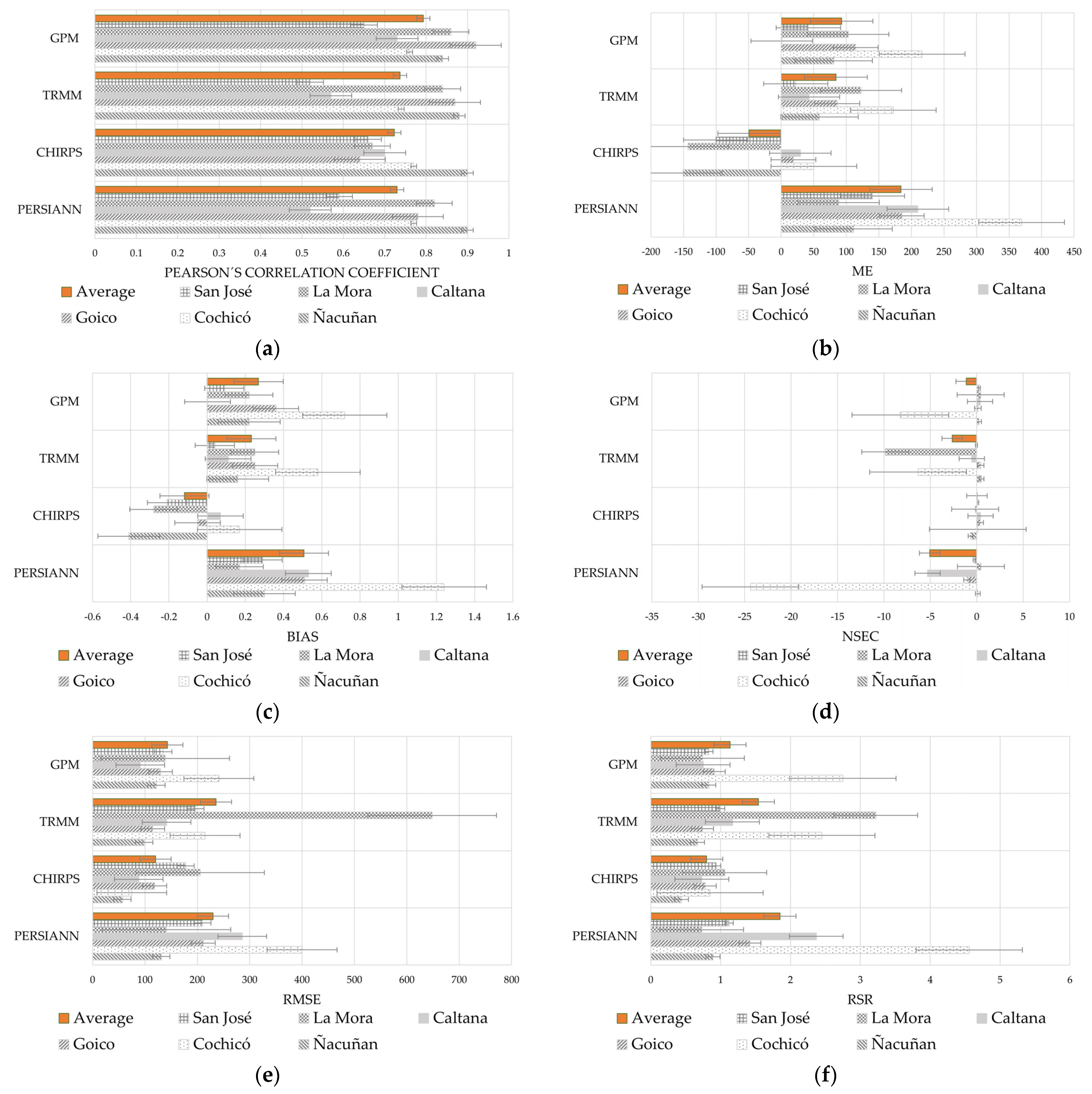
3.1. Gauged and Estimated Precipitation Comparison

The double-mass analyses indicated the consistency of all remote-sensing products. All satellite products showed linear behaviour without any break in the slope and with high correlation values (r2 > 0.99) at the six gauge stations, which ensured data consistency throughout the gathering period [48] (Figures S1–S4 in Supplementary Materials).

3.1.1. Pixel-to-Point Analysis

Indicators r, ME, Bias, RMSE, RSR, and NSEc were used to test the relation between daily, monthly and annual gauged and estimated precipitation data. Results are presented in Figure 3a–f for the monthly scale and Figure 4a–f for the annual scale and Tables S1–S12, respectively. Daily r showed lower correlations (0.14 < r < 0.65) for all the locations (Table 3); therefore, further analyses were carried out only on a monthly and annual basis.
Monthly indicators performance varied among satellite products and gauge stations. Monthly r showed good average values for GPM and TRMM and fair average values for CHIRPS and PERSIANN. In general, CHIRPS, TRMM and GPM performed better compared to PERSIAN. The higher r values were found for GPM estimate precipitation at all gauge stations (Figure 3a), ranging from 0.72 at Cochicó to 0.90 at Ñacuñan. Regarding ME, values ranged from 31 mm/month for PERSIAN at Cochicó to 0.07 mm/month for GPM at Caltana (Figure 3b). GPM and TRMM had very similar average ME, and they both overestimate precipitation at around 7 mm/month, while CHIRPS underestimates it at about 5 mm/month (Figure 3b). The most significant adjustments were found at the Caltana gauge station for CHIRPS (ME = 0.04) and GPM (ME = 0.002). Similarly, CHIRPS, TRMM and GPM showed better Bias values than PERSIANN and while CHIRPS underestimates some stations, GPM and TRMM show consistent overestimation (Figure 3c). The average values of NSEc showed acceptable performance for CHIRPS in all stations, mostly acceptable for TRMM and GPM, but very poor performance for PERSIANN (Figure 3d). At the gauge station level, the best performance of satellite estimated data was found for GPM at Ñacuñan (NSEc = 0.75) and Caltana (NSEc = 0.68). RMSE and RSR presented acceptable average values for CHIRPS, GPM and GPM and worse performance for PERSIANN. At all gauge stations, CHIRPS consistently presented values of RSR between 0 and 1 (Figure 3f). The best GPM performance occurred at Ñacuñan with the lowest RMSE (18.1) and RSR (0.50) values (Figure 3e,f).
On an annual basis, the performance of estimated precipitation against gauged data was variable among satellite products and gauge stations. The highest r was found in GPM at Goico (0.92), while the worst performance was PERSIANN at Caltana (0.52) (Figure 4a). In general, Caltana stations had the best performance with all estimated precipitation. In addition, all satellite estimated data presented good average r values, with the GPM with the highest score (Figure 4a). CHIRPS presented the lowest values of ME and Bias with a negative sign (underestimation). At the same time, TRMM and GPM also performed well when considering ME and Bias metrics but overestimated the data (Figure 4b,c). GPM at Caltana showed the best adjustment for estimated annual data with a ME of 0.89 mm and a Bias of 0.002. CHIRPS is the only product with a positive average NSEc value, while the other satellite products’ performance was only acceptable in some stations (Figure 4d). CHIRPS showed good RMSE and RSR average values compared to the other products (Figure 4f). To integrate and compare the indicators by satellite product for the six gauge stations, the average monthly and annual values are presented in Table 4 and Table 5. Best values are highlighted in bold.
At monthly timestep (Table 4), GPM presented the best correlation, RMSE, and RSR. CHIRPS resulted in lower ME and Bias, while both products showed equal accuracy according to NSEc values. On an annual basis (Table 5), CHIRPS showed the best adjustment for all indicators except for r. GPM correlated the best between gauged and estimated satellite precipitation.
Finally, the average value of the statistical metrics was calculated to determine the performance of the estimated data at each gauge station. Table 6 and Table 7 present the average statistics of the estimated data at each location at the monthly and annual levels.
Ñacuñan performed better for the statistical metrics considering the average of all satellite estimated data except for Bias, although this last value was acceptable.

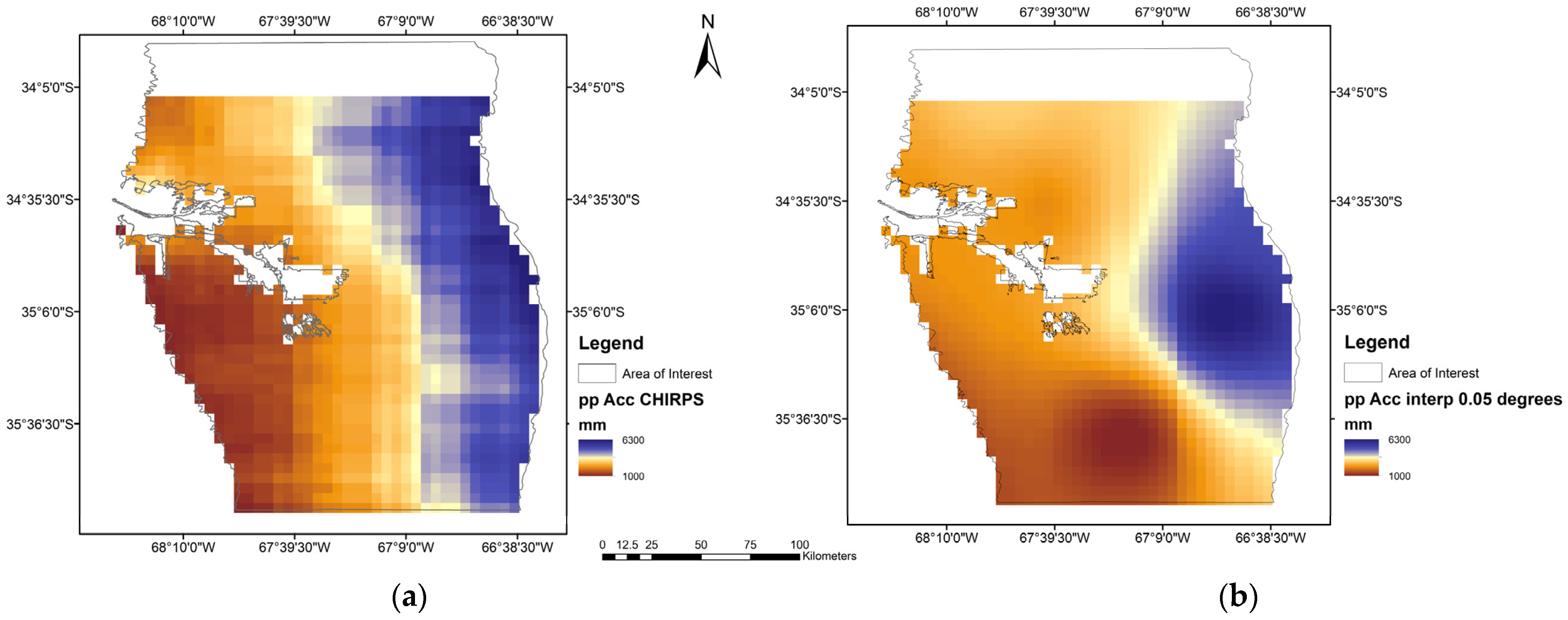
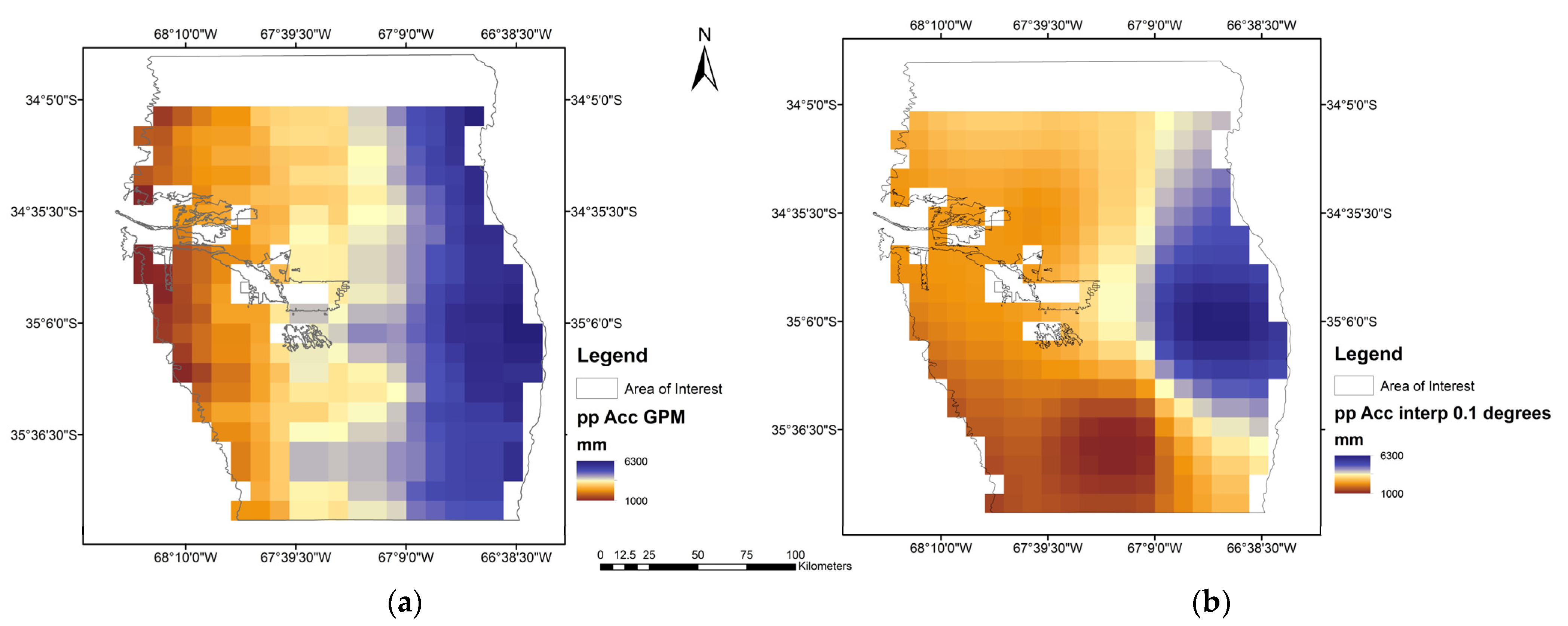
3.1.2. Pixel-to-Pixel Analysis

Pearson’s Correlation Coefficient (r) was calculated for comparing and analysing the accuracy of estimated precipitation spatially (pixel-to-pixel) against interpolated gauged data within the interest area.
Figure 5 and Figure 6 present distributed values of estimated precipitation by CHIRPS and GPM satellite and interpolated gauged data at a 0.05-degree and 0.1-degree spatial resolution, respectively, from 2008 to 2018. Figure 7 presents the distributed r between interpolated and estimated monthly precipitation by CHIRPS and GPM for the same period.
Although both satellites performed well, GPM presented a better correlation between satellite-estimated data and gauged interpolated data. For the GPM satellite, most pixels reached a high or very high correlation (r > 0.8).
Two gauge stations within the interest area, Caltana and San José, were used to validate and evaluate the correlation analysis’s consistency. Table 8 presents the PPC values for estimated data from CHIRPS, interpolated, and gauged data. Table 9 presents the results of the GPM satellite estimated precipitation.

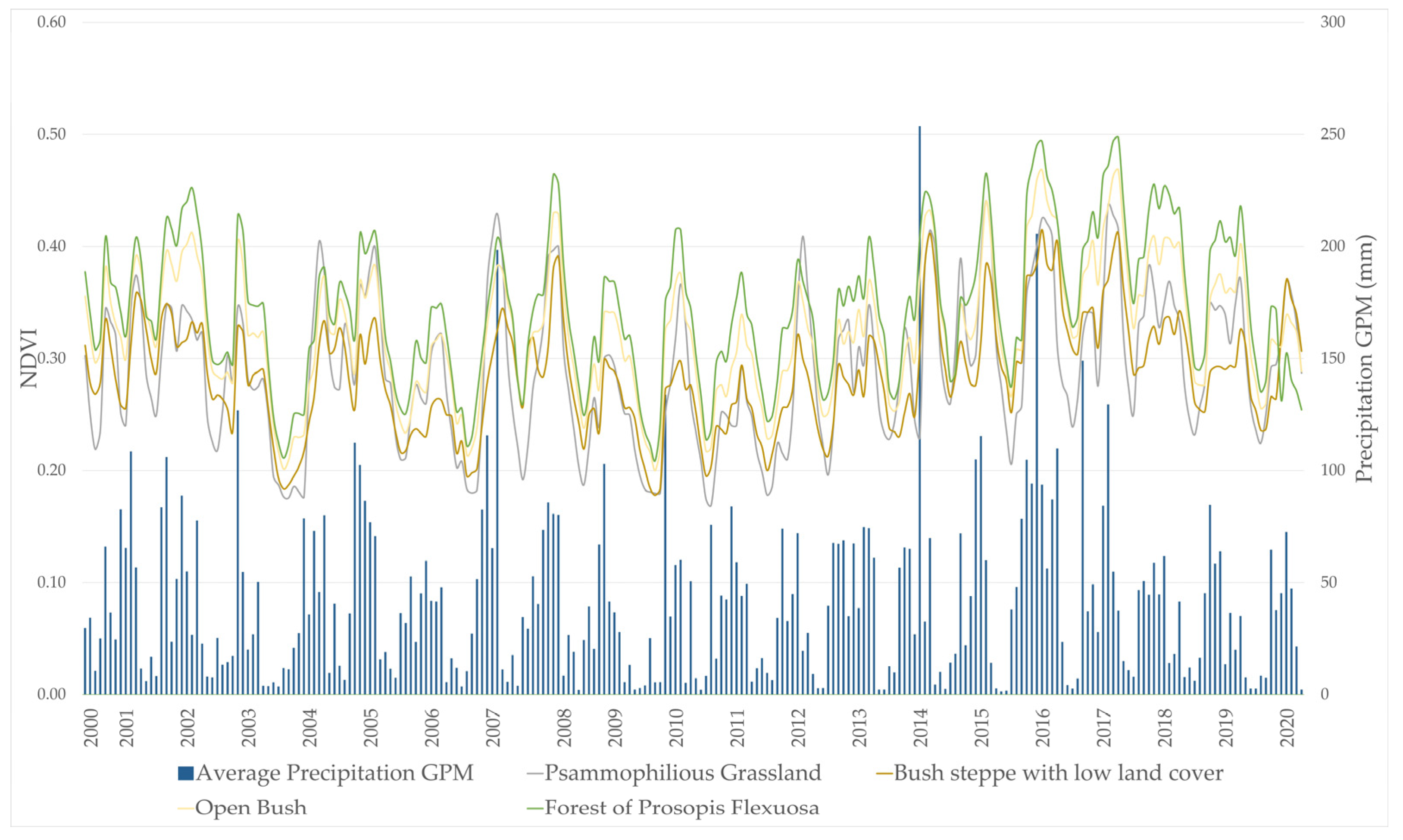
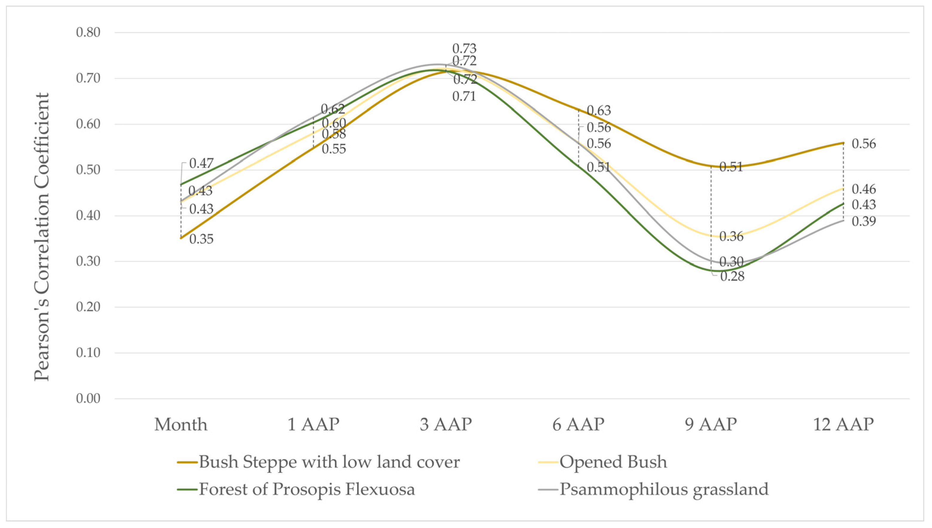
3.2. NDVI and Accumulated Antecedent Precipitation Analysis

GPM satellite estimated precipitation was then correlated to MODIS-derived NDVI at a monthly temporal scale from 2000 to 2020, considering monthly (0 AAP) and 1, 3, 6, 9 and 12 months AAP. The analysis was carried out in 100 points of each primary vegetation type of the interest area. Figure 8 shows the monthly evolution of the estimated precipitation and the NDVI for each vegetation type as the average of the points. The shape and patterns of the NDVI curves and precipitation bar show a summer seasonal vegetation growing and precipitation.
Values of r varied according to the accumulated antecedent monthly precipitation and vegetation types. Figure 9 shows the average r variation for each vegetation type as a function of AAP. All vegetation types showed a similar response and behaviour to AAP, with a higher correlation between NDVI and 3 months of AAP, followed by 1 month of AAP for Open Bush, Forest of Prosopis flexuosa, and Psammophilous grassland. It is possible to differentiate bush steppe with low land cover from the other bush types and grassland as the curve slope of this vegetation type is smoother between 6 and 12 months of AAP.
Considering ground-measured data, Figure 10 presents the correlation r for each vegetation type and AAP for the four gauged stations: Ñacuñan (a), Cochicó (b), El Goico (c), and La Mora (d).
Correlation values present differences among gauged stations and vegetation types. Lower values for Bush Steppe and Psammophilous grassland could be explained since the stations are in Open Bush and Forest of Prosopis flexuosa vegetation types. The four stations show a higher correlation for 3-months and 6-month AAP, except for Open Bush at Cochicó. Stations in Forest of Prosopis flexuosa (La Mora) and Open Bush (Ñacuñan) show similar results compared to the correlation from 100 random points and estimated precipitation (GPM).

4. Discussion

In the drylands of Mendoza, similarly to other dryland regions worldwide, few precipitation gauge data stations with long continuous series allow for suitable distributed precipitation and vegetation analysis. Satellite-estimated precipitation data are crucial and valuable for decision-making and natural resources management. However, uncertainties related to estimation methods and analytical approaches must be acknowledged and quantified to have this data translated into decision-making [30].
Estimated satellite precipitation from the four satellite products CHIRPS, GPM, TRMM, and PERSIANN are consistent throughout the gathering periods since the double-mass curves do not present significant displacement of the line from the combined points or changes in the curve slope and showed a straight linear behaviour with a high correlation (See Supplementary Materials).
The indicator r was variable among temporal scales, satellites and gauge stations. Lower r values at daily timestep can be explained by differences in how dates are assigned to satellite products and gauge stations. While satellite products are set using UTC or GTS time zones, automatic gauge stations from national networks retrieve mm/day calculated from 9 am of one day to 9 am on the following day. This noise in data matching is diluted at monthly and yearly timesteps. Then, more robust relationships between the measured and estimated precipitation data were found at monthly and annual scales. GPM showed the best performance monthly, while on an annual basis, GPM, together with CHIRPS and PERSIANN, reached high correlation values. Considering the average r, GPM presented the best correlation values. These findings are consistent with [24] who compared seven satellite-based products’ estimated precipitation in Burkina Faso. On a daily temporal scale, all the products showed a low correlation (r < 0.50). These results reversed when considering monthly and annual time steps (r > 0.80). Better performances were shown for those satellite-based products with higher spatial resolution. Increased accuracy at monthly and annual time-step was also found by Muhammad et al. [26] for satellite-based products, although with variation among climate regions. Following the performance comparison using r, the other indicators were carried out only for monthly and annual temporal scales.
ME shows the average error between measured and gauged data. One satellite product, CHIRPS, underestimates the data, while the other three overestimate the precipitation. CHIRPS presented the lower ME. However, on a monthly scale, the absolute magnitude of the difference of the mean error for TRMM and GPM compared to CHIRPS is only about 2 and 2.4 mm. Other researchers also found that most satellite-based products overestimate precipitation in South America, especially in areas with convective precipitation [32].
Bias shows to what extent measured data are underestimated or overestimated by satellite data depending on how close to 1 the values are. CHIRPS, TRMM and GPM showed a similar performance with magnitudes of difference from 1 of 0.22, 0.23 and 0.26, respectively.
CHIRPS and GPM presented the lowest absolute average error between measured and satellite-estimated data according to the RMSE at both temporal scales. These two satellites were also the best predictors of the measured data from estimates as they presented the best values of NSEc.
Gao et al. [49] compared CHIRPS and PERSIANN CDR for estimated precipitation and found that both PERSIANN and CHIRPS showed Correlation coefficients that were very similar at monthly and annual temporal scales. However, in our case, CHIRPS performed better for BIAS and RMSE. Comparing PERSIANN and CHIRPS against interpolated precipitation from gauged data, CHIRPS presented better statistics and metrics than PERSIANN, probably due to its higher spatial resolution.
Toté et al. [27] found variations comparing three satellite-estimated precipitation products in Mozambique according to the magnitude of precipitation, season, and country region. They also found that algorithms that combine TIR and PM, such as CHIRPS, had better statistical performance than those only based on TIR.
r was also calculated for comparing and analysing the accuracy of estimated precipitation from CHIRPS and GPM in a distributed extension—pixel by pixel, against interpolated gauged data within the interest area. Dembélé et al. [24] suggested carrying out this kind of pixel-to-pixel analysis to estimate the accuracy of these products for spatial precipitation patterns. GPM performed better since all the pixels reached a high or very high correlation. These findings were validated by correlating the estimated precipitation, interpolated precipitation, and gauged data at two gauge stations located within the interest area.
However, gridded precipitation data from interpolated gauged data vary according to gauge station density, distribution, and evolution over time. The accuracy of gridded and gauged data also depends on interpolation methods used, most of them based on the distance between stations. Uncertainties arise from using gridded data and employing estimated satellite precipitation data. Therefore, acknowledging and quantifying these uncertainties become significant but must not be seen as barriers to using data, especially in areas with scarce or no data [29].
In the interest area, storms occur mainly as convection episodes during spring and summer, influenced by the Andean range, air moisture, and thermal amplitude, among other factors [50]. These convective storms are spatially located; therefore, satellite-gridded estimated precipitation data are likely to fit better than interpolated data in reflecting the distributed precipitation.
MODIS-derived NDVI at a monthly temporal scale from 2000 to 2020 was correlated to GPM satellite-estimated precipitation considering monthly and 1-, 3-, 6-, 9- and 12-months AAP. This analysis in 100 points of each primary vegetation type of the interest area showed that the highest correlation between NDVI and antecedent accumulated precipitation was with 3 months AAP for all the vegetation types.
The evolution of NDVI as a function of APP showed little differences among vegetation types except for bush steppe with low land cover, which presented a smoothed curve for 6-, 9- and 12-months AAP. This similarity in the curve shapes can be partly explained because the area belongs to the same phytogeography region of “Monte” and has many typical species of semi-arid ecosystems in common.
Considering the correlation between NDVI and AAP from individual gauge stations, higher values were found with 3-month and 6-month AAP for the four vegetation types. Comparing the results of correlations from estimated and measured AAP, the differences could be partly explained by the length of the data available and that ground stations are in two of the four vegetation types.
These arid and semi-arid bushlands share the characteristic of having most of the root systems up to 1 m depth, which makes them more sensitive to short-term changes in soil moisture [7]. Previous studies analysing the vegetation fractions’ dependence on antecedent accumulated precipitation for Australia found the best response of photosynthetic fraction cover for an accumulated period lower than 12 months AAP [21]. Other researchers in arid rangelands also found a higher correlation between NDVI and AAP between three months during summer and up to six months in winter [51]. These variations in ecosystem productivity measured through NDVI associated with changes in AAP and then to water availability were also found in dryland globally but more significant in the southern hemisphere [3]. However, spatial scales of analysis and land use management must be considered in comparing patterns of responses of vegetation to antecedent accumulated precipitation.
For cattle grazing management based on natural vegetation, the relationship between NDVI, biomass, and precipitation result is essential for the production’s sustainability and avoiding overgrazing. Estimated precipitation such as satellite products was not assessed in this region, especially considering that storms present a highly uneven spatial distribution due to their convective nature [50]. Furthermore, for livestock farming, forage availability is critical in decision-making in terms of managing the calves/cows ratio and when to discharge the field. In dry areas where vegetation and animal growth are sensitive to precipitation changes, the availability of reliable and timely precipitation data would support a decision system and develop adaptation management practices considering climate change and variability [19]. Lack of precipitation-gauged data or having them spatially and temporally sparse and fragmented is a barrier to sustainably managing natural resources and production systems and building decision support systems according to environmental conditions. Remote-sensing-estimated precipitation was successfully applied in areas with little observed or gauged data, especially in developing countries [24,25,26,27] or over great extensions without a dense gauge network, such as China and Australia [28].

5. Conclusions

This paper aimed to determine the relationship between NDVI and AAP in natural dryland vegetation types as a basis for decision support in cattle grazing. In doing so and considering the lack of reliable and continuous precipitation data, firstly, observed and estimated precipitation data from remote sensing were compared to evaluate its suitability and accuracy as a tool for analysing climate parameters and vegetation index in areas with scarce gauged data, such as the drylands of Mendoza. Secondly, estimated and gauged AAP precipitation was correlated to NDVI in four vegetation types.
Results from correlating NDVI and AAP showed a high association between natural vegetation productivity and precipitation. CHIRPS and GPM showed accuracy at monthly and annual temporal scales according to the evaluated statistics and metrics, making them valuable and reliable for considering these estimated data in models and analyses. Based on the findings of this paper regarding the relationship between NDVI and AAP, farmers must consider the accumulated precipitation of 3 months of AAP rather than the current or previous month’s precipitation for livestock management.
Satellite-estimated precipitation correlated better than interpolated precipitation from gauge stations, probably due to the convective nature of the summer storms. CHIRPS has a higher spatial resolution given by a 0.05-degree pixel against 0.1-degree for GPM, which confers a more significant source of information. However, GPM would better inform early warning systems or management decisions such as forage forecasting in livestock because of its quasi-real-time availability (two or three days) at Google Earth Engine (GEE) image collection catalogues, compared to CHIRPS, which is available between 1 and 2 months later.
Limitations of this methodology may arise due to limited data processing capacity, consistency of gauged precipitation data, and timely access to information. Although the findings of this work apply to southeast Mendoza, methodologically, they can be extrapolated to other areas with scarce or fragmented precipitation information. Free access to the estimated precipitation dataset is an asset that becomes essential when combined with NDVI data to support decision-making for livestock farmers in areas with no gauged information.
In conclusion, estimated precipitation data from GPM and CHIRPS satellites are accurate and valuable for analysing the relationships between precipitation and other different factors related to vegetation growth and status, such as NDVI, natural resources management, bushfires warnings, droughts, precipitation use efficiency, and as input for a decision support system in drylands of Mendoza, Argentina.
Further studies considering water availability during the growing season of each vegetation type are needed to have a deeper understanding of vegetation dynamics and to enhance the tool for natural pasture management.

Supplementary Materials

The following supporting information can be downloaded at: https://www.mdpi.com/article/10.3390/rs15143615/s1, Figures S1–S4 present the Double Mass Analyses for the four satellite products at the gauge stations locations. Tables S1–S12 present the annual and monthly statistics by gauged and satellite-estimated precipitation for Pearson’s Correlation Coefficient (r); Mean Error (ME); Bias; Nash–Sutcliffe Efficiency Coefficient (NSEC); Root Mean Square Error (RMSE); and RMSE-observations standard deviation ratio (RSR).

Author Contributions

C.B. and J.F.R. designed the research, C.B. performed the data analysis, processed remote sensing data and wrote the manuscript, J.F.R., P.M.S., S.G.S. and S.M. significantly contributed to study design, result analysis and discussion, and manuscript refinement. All authors have read and agreed to the published version of the manuscript.

Funding

This research was funded by the University of Newcastle by a Postgraduate Research Scholarship for C.B.

Data Availability Statement

The dataset analysed during this study can be found at ee.ImageCollection (“TRMM/3B42”); ee.ImageCollection (“NASA/GPM_L3/IMERG_V06); ee.ImageCollection (“UCSB-CHG/CHIRPS/DAILY)”; ee.ImageCollection (“NOAA/PERSIANN-CDR”); https://www.mendoza-conicet.gob.ar/ladyot/red_iadiza/index.html, accessed on 10 August 2020; https://www.argentina.gob.ar/obras-publicas/hidricas/base-de-datos-hidrologica-integrada, accessed on 5 August 2020.

Acknowledgments

This research was carried out in the framework of the University of Newcastle HDR Program in Environmental Engineering through the 2020 VCHDR Vice Chancellor’s HDR Training scholarship. It was also supported by the National Institute of Agriculture Technology (INTA) of Argentina (www.inta.gob.ar).

Conflicts of Interest

The authors declare no conflict of interest.

References

  1. Saco, P.M.; Willgoose, G.R.; Hancock, G.R. Eco-geomorphology of banded vegetation patterns in arid and semi-arid regions. Hydrol. Earth Syst. Sci. 2007, 11, 1717–1730. [Google Scholar] [CrossRef] [Green Version]
  2. Saco, P.M.; Moreno-de las Heras, M. Ecogeomorphic coevolution of semiarid hillslopes: Emergence of banded and striped vegetation patterns through interaction of biotic and abiotic processes. Water Resour. Res. 2013, 49, 115–126. [Google Scholar] [CrossRef]
  3. Zhao, W.; Yu, X.; Xu, C.; Li, S.; Wu, G.; Yuan, W. Dynamic traceability effects of soil moisture on the precipitation–vegetation association in drylands. J. Hydrol. 2022, 615, 128645. [Google Scholar] [CrossRef]
  4. Tian, S.; Van Dijk, A.I.J.M.; Tregoning, P.; Renzullo, L.J. Forecasting dryland vegetation condition months in advance through satellite data assimilation. Nat. Commun. 2019, 10, 469. [Google Scholar] [CrossRef] [PubMed] [Green Version]
  5. Almalki, R.; Khaki, M.; Saco, P.M.; Rodriguez, J.F. Monitoring and Mapping Vegetation Cover Changes in Arid and Semi-Arid Areas Using Remote Sensing Technology: A Review. Remote Sens. 2022, 14, 5143. [Google Scholar] [CrossRef]
  6. Zeng, L.; Wardlow, B.D.; Xiang, D.; Hu, S.; Li, D. A review of vegetation phenological metrics extraction using time-series, multispectral satellite data. Remote Sens. Environ. 2020, 237, 111511. [Google Scholar] [CrossRef]
  7. Joiner, J.; Yoshida, Y.; Anderson, M.; Holmes, T.; Hain, C.; Reichle, R.; Koster, R.; Middleton, E.; Zeng, F.-W. Global relationships among traditional reflectance vegetation indices (NDVI and NDII), evapotranspiration (ET), and soil moisture variability on weekly timescales. Remote Sens. Environ. 2018, 219, 339–352. [Google Scholar] [CrossRef]
  8. Ruppert, J.C.; Holm, A.; Miehe, S.; Muldavin, E.; Snyman, H.A.; Wesche, K.; Linstädter, A. Meta-analysis of ANPP and rain-use efficiency confirms indicative value for degradation and supports non-linear response along precipitation gradients in drylands. J. Veg. Sci. 2012, 23, 1035–1050. [Google Scholar] [CrossRef]
  9. Zhao, Y.; Wang, X.; Vázquez-Jiménez, R. Evaluating the performance of remote sensed rain-use efficiency as an indicator of ecosystem functioning in semi-arid ecosystems. Int. J. Remote Sens. 2018, 39, 3344. [Google Scholar] [CrossRef]
  10. Baldassini, P.; Volante, J.N.; Califano, L.M.; Paruelo, J.M. Caracterización regional de la estructura y de la productividad de la vegetación de la Puna mediante el uso de imágenes MODIS / Regional characterization of the structure and productivity of the vegetation of the Puna using MODIS images. Ecol. Austral 2012, 22, 22–32. [Google Scholar]
  11. Qin, X.-J.; Hong, J.-T.; Ma, X.-X.; Wang, X.-D. Global patterns in above-ground net primary production and precipitation-use efficiency in grasslands. J. Mt. Sci. 2018, 15, 1682–1692. [Google Scholar] [CrossRef]
  12. Saco, P.M.; Moreno-de las Heras, M.; Keesstra, S.; Baartman, J.; Yetemen, O.; Rodríguez, J.F. Vegetation and soil degradation in drylands: Non linear feedbacks and early warning signals. Curr. Opin. Environ. Sci. Health 2018, 5, 67–72. [Google Scholar] [CrossRef]
  13. Saco, P.M.; Rodríguez, J.F.; Moreno-de las Heras, M.; Keesstra, S.; Azadi, S.; Sandi, S.; Baartman, J.; Rodrigo-Comino, J.; Rossi, M.J. Using hydrological connectivity to detect transitions and degradation thresholds: Applications to dryland systems. CATENA 2020, 186, 104354. [Google Scholar] [CrossRef]
  14. López-Pérez, A.; Martínez-Menes, M.R.; Fernández-Reynoso, D.S. Priorización de áreas de intervención mediante análisis morfométrico e índice de vegetación. Technol. Cienc. Agua 2015, 6, 121–137. [Google Scholar]
  15. Pasquarella, V.J.; Holden, C.E.; Woodcock, C.E. Improved mapping of forest type using spectral-temporal Landsat features. Remote Sens. Environ. 2018, 210, 193–207. [Google Scholar] [CrossRef]
  16. Blanco, L.J.; Paruelo, J.M.; Oesterheld, M.; Biurrun, F.N.; Rocchini, D. Spatial and temporal patterns of herbaceous primary production in semi-arid shrublands: A remote sensing approach. J. Veg. Sci. 2016, 27, 716. [Google Scholar] [CrossRef]
  17. Jiapaer, G.; Chen, X.; Bao, A. A comparison of methods for estimating fractional vegetation cover in arid regions. Agric. For. Meteorol. 2011, 151, 1698–1710. [Google Scholar] [CrossRef]
  18. Sandi, S.G.; Rodriguez, J.F.; Saintilan, N.; Wen, L.; Kuczera, G.; Riccardi, G.; Saco, P.M. Resilience to drought of dryland wetlands threatened by climate change. Sci. Rep. 2020, 10, 13232. [Google Scholar] [CrossRef]
  19. Souza, R.; Hartzell, S.; Feng, X.; Dantas Antonino, A.C.; de Souza, E.S.; Cezar Menezes, R.S.; Porporato, A. Optimal management of cattle grazing in a seasonally dry tropical forest ecosystem under rainfall fluctuations. J. Hydrol. 2020, 588, 125102. [Google Scholar] [CrossRef]
  20. Hill, M.J.; Guerschman, J.P. The MODIS Global Vegetation Fractional Cover Product 2001–2018: Characteristics of Vegetation Fractional Cover in Grasslands and Savanna Woodlands. Remote Sens. 2020, 12, 406. [Google Scholar] [CrossRef] [Green Version]
  21. Guerschman, J.P.; Hill, M.J.; Leys, J.; Heidenreich, S. Vegetation cover dependence on accumulated antecedent precipitation in Australia: Relationships with photosynthetic and non-photosynthetic vegetation fractions. Remote Sens. Environ. 2020, 240, 111670. [Google Scholar] [CrossRef]
  22. Li, H.; Wei, X.; Zhou, H. Rain-use efficiency and NDVI-based assessment of karst ecosystem degradation or recovery: A case study in Guangxi, China. Environ. Earth Sci. 2015, 74, 977–984. [Google Scholar] [CrossRef]
  23. Ma, J.; Jia, X.; Zha, T.; Bourque, C.P.A.; Tian, Y.; Bai, Y.; Liu, P.; Yang, R.; Li, C.; Li, C.; et al. Ecosystem water use efficiency in a young plantation in Northern China and its relationship to drought. Agric. For. Meteorol. 2019, 275, 1–10. [Google Scholar] [CrossRef]
  24. Dembélé, M.; Zwart, S.J. Evaluation and comparison of satellite-based rainfall products in Burkina Faso, West Africa. Int. J. Remote Sens. 2016, 37, 3995–4014. [Google Scholar] [CrossRef] [Green Version]
  25. Banerjee, A.; Chen, R.; Meadows, M.E.; Singh, R.B.; Mal, S.; Sengupta, D. An Analysis of Long-Term Rainfall Trends and Variability in the Uttarakhand Himalaya Using Google Earth Engine. Remote Sens. 2020, 12, 709. [Google Scholar] [CrossRef] [Green Version]
  26. Muhammad, E.; Muhammad, W.; Ahmad, I.; Muhammad Khan, N.; Chen, S. Satellite precipitation product: Applicability and accuracy evaluation in diverse region. Sci. China Technol. Sci. 2020, 63, 819–828. [Google Scholar] [CrossRef]
  27. Toté, C.; Patricio, D.; Boogaard, H.; Van der Wijngaart, R.; Tarnavsky, E.; Funk, C. Evaluation of Satellite Rainfall Estimates for Drought and Flood Monitoring in Mozambique. Remote Sens. 2015, 7, 1758–1776. [Google Scholar] [CrossRef] [Green Version]
  28. Woldemeskel, F.M.; Sivakumar, B.; Sharma, A. Merging gauge and satellite rainfall with specification of associated uncertainty across Australia. J. Hydrol. 2013, 499, 167–176. [Google Scholar] [CrossRef]
  29. Tozer, C.R.; Kiem, A.S.; Verdon-Kidd, D.C. On the uncertainties associated with using gridded rainfall data as a proxy for observed. Hydrol. Earth Syst. Sci. 2012, 16, 1481–1499. [Google Scholar] [CrossRef] [Green Version]
  30. Kiem, A.S.; Austin, E.K.; Verdon-Kidd, D.C. Water resource management in a variable and changing climate: Hypothetical case study to explore decision making under uncertainty. J. Water Clim. Chang. 2015, 7, 263–279. [Google Scholar] [CrossRef]
  31. Gibson, A.J.; Verdon-Kidd, D.C.; Hancock, G.R.; Willgoose, G. Catchment-scale drought: Capturing the whole drought cycle using multiple indicators. Hydrol. Earth Syst. Sci. 2020, 24, 1985–2002. [Google Scholar] [CrossRef] [Green Version]
  32. Sun, Q.; Miao, C.; Duan, Q.; Ashouri, H.; Sorooshian, S.; Hsu, K.-L. A Review of Global Precipitation Data Sets: Data Sources, Estimation, and Intercomparisons. Rev. Geophys. 2018, 56, 79–107. [Google Scholar] [CrossRef] [Green Version]
  33. Abraham, E.; del Valle, H.F.; Roig, F.; Torres, L.; Ares, J.O.; Coronato, F.; Godagnone, R. Overview of the geography of the Monte Desert biome (Argentina). J. Arid Environ. 2009, 73, 144–153. [Google Scholar] [CrossRef]
  34. Cruzate, G.; Gomez, L.; Pizarro, M.J.; Mercuri, P.; Banchero, S. Suelos de la República Argentina. SAGyP-INTA-Proy. PNUD ARG/85/019; 2007. Available online: http://www.geointa.inta.gob.ar/2013/05/26/suelos-de-la-republica-argentina/ (accessed on 18 March 2020).
  35. Abraham, E. Geomorfología de la Provincia de Mendoza. Argent. Recur. Y Probl. Ambient. De La Zona Árida 2000, 29–48. Available online: https://www.researchgate.net/publication/285798616_Geomorfologia_de_la_Provincia_de_Mendoza (accessed on 5 April 2020).
  36. Cabrera, A.L. Regiones Fitogeográficas Argentinas. In Enciclopedia Argentina de Agricultura y Jardinería; ACME SACI: Buenos Aires, Argentina, 1976; Volume 2, p. 85. [Google Scholar]
  37. MAyDS, I.-P. Manejo Sustentable de Tierras en las Zonas Secas del Noroeste Argentino. PNUD ARG/14/G55. Tech. Rep. PNUD Third Progress Report; 2020; p. 158. Available online: https://inta.gob.ar/sites/default/files/pnud_arg_14_g55_avance_informe_3_version_final.pdf (accessed on 20 December 2020).
  38. Mora, S.; Orozco, A.; Eraso, V.y.; Montecinos, F. Evaluación de alternativas tecnológicas para Ia recuperación de pastizales psamofitos en el sur de Mendoza. Rev. Argent. Prod. Anim. 2008, 28, 194. [Google Scholar]
  39. Olmedo, G.; Vallone, R.; Tacchini, F.; Naldini, E. Zonificación de la Vegetación y de Áreas Ganaderas de la Zona Árida del Departamento de General Alvear. 2014, pp. 23–36. Available online: https://www.researchgate.net/publication/278668151_Zonificacion_de_la_vegetacion_y_de_Areas_Ganaderas_de_la_Zona_Arida_del_Departamento_de_General_Alvear (accessed on 27 February 2020).
  40. Mendoza, C.G.D. Caracterización 2019. Ministerio de Economía y Energía; Subsecretría de A.Y.G., Ed.; Cluster Ganadero de Mendoza: Mendoza, Argentina, 2019; p. 21. [Google Scholar]
  41. Didan, K. MOD13Q1 MODIS/Terra Vegetation Indices 16-Day L3 Global 250m SIN Grid V006; Daac, N.E.L.P., Ed.; NASA: Washington, DC, USA, 2015. Available online: https://lpdaac.usgs.gov (accessed on 4 August 2020).
  42. Huffman, G.J.; Stocker, E.F.; Bolvin, D.T.; Nelkin, E.J.; Tan, J. GPM IMERG Final Precipitation L3 1 Month 0.1 Degree x 0.1 Degree V06; NASA: Washington, DC, USA, 2019. Available online: https://disc.gsfc.nasa.gov/datasets/GPM_3IMERGM_06/summary (accessed on 14 August 2020).
  43. Adler, R.F.; Sapiano, M.; Huffman, G.J.; Wang, J.; Gu, G.; Bolvin, D.; Chiu, L.; Schneider, U.; Becker, A.; Nelkin, E.; et al. The Global Precipitation Climatology Project (GPCP) Monthly Analysis (New Version 2.3) and a Review of 2017 Global Precipitation. Atmosphere 2018, 9, 138. [Google Scholar] [CrossRef]
  44. Funk, C.; Peterson, P.; Landsfeld, M.; Pedreros, D.; Verdin, J.; Shukla, S.; Husak, G.; Rowland, J.; Harrison, L.; Hoell, A.; et al. The climate hazards infrared precipitation with stations—A new environmental record for monitoring extremes. Sci. Data 2015, 2, 150066. [Google Scholar] [CrossRef] [Green Version]
  45. Ashouri, H.; Hsu, K.-L.; Sorooshian, S.; Braithwaite, D.K.; Knapp, K.R.; Cecil, L.D.; Nelson, B.R.; Prat, O.P. PERSIANN-CDR: Daily Precipitation Climate Data Record from Multisatellite Observations for Hydrological and Climate Studies. Bull. Am. Meteorol. Soc. 2015, 96, 69–83. [Google Scholar] [CrossRef] [Green Version]
  46. Duan, Z.; Bastiaanssen, W.G.M.; Liu, J. Monthly and annual validation of TRMM Mulitisatellite Precipitation Analysis (TMPA) products in the Caspian Sea Region for the period 1999–2003. In Proceedings of the IEEE International Geoscience and Remote Sensing Symposium, Munich, Germany, 22–27 July 2012; pp. 3696–3699. [Google Scholar] [CrossRef]
  47. Moriasi, D.N.; Arnold, J.G.; Van Liew, M.W.; Bingner, R.L.; Harmel, R.D.; Veith, T.L. Model Evaluation Guidelines for Systematic Quantification of Accuracy in Watershed Simulations. Trans. ASABE 2007, 50, 885–900. [Google Scholar] [CrossRef]
  48. Ponce, V.M. Engineering Hydrology: Principles and Practices; Prentice Hall: Englewood Cliffs, NJ, USA, 1989; Volume 640. [Google Scholar]
  49. Gao, F.; Zhang, Y.; Chen, Q.; Wang, P.; Yang, H.; Yao, Y.; Cai, W. Comparison of two long-term and high-resolution satellite precipitation datasets in Xinjiang, China. Atmos. Res. 2018, 212, 150–157. [Google Scholar] [CrossRef]
  50. Calori, A.; Santos, J.R.; Blanco, M.; Pessano, H.; Llamedo, P.; Alexander, P.; de la Torre, A. Ground-based GNSS network and integrated water vapor mapping during the development of severe storms at the Cuyo region (Argentina). Atmos. Res. 2016, 176–177, 267–275. [Google Scholar] [CrossRef]
  51. Long, X.; Guan, H.; Sinclair, R.; Batelaan, O.; Facelli, J.M.; Andrew, R.L.; Bestland, E. Response of vegetation cover to climate variability in protected and grazed arid rangelands of South Australia. J. Arid. Environ. 2019, 161, 64–71. [Google Scholar] [CrossRef]
Figure 1. Vegetation types according to the functional classification. Relatives: (a) Argentina, (b) Mendoza province.
Remotesensing 15 03615 g001
Figure 2. Location of Gauge Stations used in the study (interpolation and validation). Inserts: (a) Argentina, (b) Mendoza province.
Remotesensing 15 03615 g002
Figure 3. Monthly indicators by gauged and satellite estimated precipitation for (a) Pearson’s Correlation Coefficient (r); (b) Mean Error (ME); (c) Bias; (d) Nash–Sutcliffe Efficiency Coefficient (NSEC); (e) Root Mean Square Error (RMSE); and (f) RMSE-observations standard deviation ratio (RSR).
Remotesensing 15 03615 g003aRemotesensing 15 03615 g003b
Figure 4. Annual statistics by gauged and satellite estimated precipitation for (a) Pearson’s Correlation Coefficient (r); (b) Mean Error (ME); (c) Bias; (d) Nash–Sutcliffe Efficiency Coefficient (NSEC); (e) Root Mean Square Error (RMSE); and (f) RMSE-observations standard deviation ratio (RSR).
Remotesensing 15 03615 g004
Figure 5. Distributed values of estimated precipitation using CHIRPS and interpolated data. (a) Accumulated estimated precipitation using CHIRPS and (b) Accumulated interpolated precipitation data at 0.05 degrees.
Remotesensing 15 03615 g005
Figure 6. Distributed values of estimated precipitation using GPM and interpolated data at 0.1 degrees. (a) Accumulated estimated precipitation using GPM and (b) Accumulated interpolated precipitation data at 0.1 degrees.
Remotesensing 15 03615 g006
Figure 7. Distributed Pearson’s Correlation Coefficient between interpolated gauged data. (a) Estimated precipitation using CHIRPS, and (b) estimated precipitation using GPM.
Remotesensing 15 03615 g007
Figure 8. Monthly average Precipitation and NDVI evolution for the vegetation type.
Remotesensing 15 03615 g008
Figure 9. Average Pearson’s Correlation Coefficient for Vegetation type and Accumulated Antecedent Precipitation.
Remotesensing 15 03615 g009
Figure 10. Average Pearson’s Correlation Coefficient for Vegetation type and Accumulated Antecedent Precipitation measured in gauge stations (a) Ñacuñan, (b) Cochicó, (c) El Goico, and (d) La Mora.
Remotesensing 15 03615 g010
Table 1. Gauge stations information.
Gauge StationsData AvailabilityProvider/SourceSpatial ResolutionObserved Precipitation
Ñacuñan *2008-05-01/2019-08-23IADIZAPointmm/day
Ñacuñan *1919–2019IADIZAPointmm/month
El Goico *1993-01-01/2019-12-31NSHIPointmm/day
Puesto La Mora *1983-07-01/2020-06-30NSHIPointmm/day
San Jose **1984-01/2019-03Local farmerPointmm/month
Caltana **2011-01-01/2020-07-31Local farmerPointmm/day
Cochicó *2008-09-10/2019-08-22IADIZAPointmm/day
Rama Caída***01-09-1968–todayINTAPointmm/day
Puesto Marfil ***01-11-2008/31-07-2019NSHIPointmm/day
Navia ***01-08-2002/31-03-2021NSHIPointmm/day
* Pixel-to-point and Interpolation; ** Pixel-to-point and validation pixel-to-pixel; *** Used only for interpolation.
Table 2. Image collections information.
Image CollectionsData
Availability
Provider/SourceSpatial ResolutionTemporal ResolutionEstimated Precipitation
TRMM Daily/Monthly1998-01-01NASA
ee.ImageCollection(“TRMM/3B42”)
0.25 degrees3-hmm/h
GPM Daily/Monthly2000-06-01NASA
ee.ImageCollection(“NASA/GPM_L3/IMERG_V06”)
0.1 degrees30 min/3 h/dailymm/h
CHIRPS1981-01-01UCSB/CHG
ee.ImageCollection(“UCSB-CHG/CHIRPS/DAILY”)
0.05 degreesDailymm/day
PERSIANN1983-01-01NOAA
UC-IRVINE/CHRS
ee.ImageCollection(“NOAA/PERSIANN-CDR”)
0.25 degreesDailymm/day
Table 3. Daily Pearson’s Correlation Coefficient between gauged and satellite-estimated precipitation.
ÑacuñanCochicóGoicoCaltanaLa Mora
PERSIANN0.340.300.290.140.32
CHIRPS0.320.390.250.140.24
TRMM 0.630.440.290.220.36
GPM 0.650.440.350.350.40
Table 4. Monthly Pearson’s Correlation Coefficient (r), Mean Error (ME), Bias, Nash–Sutcliffe Efficiency Coefficient (NSEC), Root Mean Square Error (RMSE), and RMSE-observations standard deviation ratio (RSR) by satellite product averaged over all gauge stations.
rMEBIASNSECRMSERSR
PERSIANN0.6215.580.42−0.3038.971.15
CHIRPS0.68−4.91−0.120.3930.230.78
TRMM0.746.940.230.2131.880.86
GPM0.787.320.260.3926.740.75
Table 5. Annual Pearson’s Correlation Coefficient (r), Mean Error (ME), Bias, Nash–Sutcliffe Efficiency Coefficient (NSEC), Root Mean Square Error (RMSE), and RMSE-observations standard deviation ratio (RSR) by satellite product averaged over all gauge stations.
rMEBIASNSECRMSERSR
PERSIANN0.73183.970.51−5.07229.841.85
CHIRPS0.72−49.25−0.120.03120.260.80
TRMM0.7484.140.23−2.64235.611.54
GPM0.7992.910.27−1.13142.861.13
Table 6. Monthly Pearson’s Correlation Coefficient (r), Mean Error (ME), Bias, Nash–Sutcliffe Efficiency Coefficient (NSEC), Root Mean Square Error (RMSE), and RMSE-observations standard deviation ratio (RSR) by gauge station averaged over all satellite products.
rMEBIASNSECRMSERSR
Ñacuñan0.831.62−0.090.5623.350.66
Cochicó0.6716.870.68−0.5634.201.21
Goico0.677.610.270.2429.860.96
Caltana0.606.080.18−0.0933.941.00
La Mora0.792.910.080.5432.020.67
San Jose0.662.300.060.3338.380.82
Table 7. Annual Pearson’s Correlation Coefficient (r), Mean Error (ME), Bias, Nash–Sutcliffe Efficiency Coefficient (NSEC), Root Mean Square Error (RMSE), and RMSE-observations standard deviation ratio (RSR) by gauge station averaged over all satellite products.
rMEBIASNSECRMSERSR
Ñacuñan0.8825.030.070.05102.080.71
Cochicó0.76202.050.68−9.71232.702.65
Goico0.80101.170.27−0.03143.460.96
Caltana0.6370.740.18−1.27151.581.25
La Mora0.8042.730.09−2.29283.401.44
San Jose0.6125.940.050.02179.630.97
Table 8. Pearson’s Correlation Coefficient among monthly estimated data from CHIRPS, interpolated data, and gauged data on a pixel-to-pixel and pixel-to-point basis at Caltana and San Jose gauge stations.
Caltana CHIRPSCaltana Gauge San José CHIRPSSan José Gauge
Caltana Gauge0.651San José gauge0.681
Caltana interpolated0.880.71San José interpolated0.830.76
Table 9. Pearson’s Correlation Coefficient among monthly estimated data from GPM, interpolated data, and gauged data on a pixel-to-pixel and pixel-to-point basis at Caltana and San Jose gauge stations.
Caltana GPMCaltana Gauge San José GPMSan José Gauge
Caltana Gauge0.741San José gauge0.721
Caltana interpolated0.890.71San José interpolated0.830.77
Disclaimer/Publisher’s Note: The statements, opinions and data contained in all publications are solely those of the individual author(s) and contributor(s) and not of MDPI and/or the editor(s). MDPI and/or the editor(s) disclaim responsibility for any injury to people or property resulting from any ideas, methods, instructions or products referred to in the content.

