Article

Monitoring Individual Tree Phenology in a Multi-Species Forest Using High Resolution UAV Images

by
Jasper Kleinsmann
1,2,*,
Jan Verbesselt
3 and
Lammert Kooistra
1
1
Laboratory of Geo-Information Science and Remote Sensing, Wageningen University and Research, 6700 AA Wageningen, The Netherlands
2
World Agroforestry, Nairobi 00100, Kenya
3
Belgian Science Policy Office (BELSPO), 1000 Brussels, Belgium
*
Author to whom correspondence should be addressed.
Remote Sens. 2023, 15(14), 3599; https://doi.org/10.3390/rs15143599
Submission received: 5 June 2023 / Revised: 12 July 2023 / Accepted: 16 July 2023 / Published: 19 July 2023
(This article belongs to the Special Issue Remote Sensing for Vegetation Phenology in a Changing Environment)

Abstract

:
Monitoring tree phenology is important for understanding ecosystem functioning and for assessing ecosystem responses to climate change. Satellite imagery offers open-access global coverage but is restricted to forest-level analyses, due to its coarse spatial resolution. Unmanned aerial vehicle (UAV) imagery can monitor phenology at the individual tree level by utilizing a centimeter-scale resolution. Two research objectives were identified for this study: (1) to derive phenological metrics at the individual tree level, using various vegetation indices (VIs); and (2) to assess the accuracy of automatic crown delineation in a diverse ecosystem. To achieve this, fourteen multi-spectral UAV flights were performed, and the ability of the normalized difference vegetation index (NDVI), enhanced vegetation index 2 (EVI2), optimized soil-adjusted vegetation index (OSAVI), and chlorophyll index red-edge (CIre) to model seasonal phenology was assessed. A double logistic model was fitted on the VI observations for each individual tree, to derive the start of season (SOS) and end of season (EOS). Individual tree crowns were delineated automatically using marker-controlled watershed segmentation (MCWS), and the treetops were identified using a local maximum filter (LMF). Overall, the automatic segmentation performed well (F-score: 0.79, IoU: 0.58), with higher accuracies in single-species areas, while it underperformed in complex mixed forest structures. All VIs captured a strong seasonal signal for the deciduous trees and derived SOS and EOS estimates consistent with literature and ground observations. General phenological patterns included an early silver birch SOS, a quick beech budburst, and large within-species phenology variations for oak trees. Seasonal VI variation for coniferous evergreen trees was limited, and the resulting phenology estimates proved unreliable. In conclusion, these findings emphasize the capabilities of UAV imagery for individual tree crown phenology monitoring. However, they also show the difficulty of monitoring evergreen phenology with the commonly-used VIs and stress the need for further investigations.

1. Introduction

Forest phenology relates to the continuous annual growth cycles of trees and is largely in sync with the seasons [1]. In temperate regions, this process is predominantly driven by temperature but also by photoperiod and water availability [2]. Hence, climate change affects ecosystem phenology through changing temperatures and precipitation [3,4]. Many studies have demonstrated an earlier start of season (SOS) as a result of global warming, and, to a lesser extent, this has been coupled with a delayed occurrence of autumn leaf senescence (end of season-EOS) [5]. The Intergovernmental Panel for Climate Change (IPCC) found an advanced onset of 2.3–5.2 days per decade globally since the 1970s [6]. In temperate and boreal forests, this rate may lie even higher, with 1.8–7.8 days per decade according to some studies [7]. This makes forest phenology a relevant indicator of climate change and is believed by some to be one of the most effective approaches to tracking climate change-induced changes in ecology [6].
Satellite-based phenology monitoring studies have been applied at forest [8,9,10,11], continental [12,13], and global scales [14,15]. However, satellites are subject to inherent limitations from weather conditions and coarse spatial and temporal resolutions [16,17]. Especially in mixed species environments, satellite-derived phenology tracking is challenging, as the satellite pixel generally exceeds the size of individual tree crowns [18]. Therefore, satellite-based phenology research is restricted to the ecosystem scale, as it is typically considered unsuitable for individual tree or species level phenology monitoring [19]. Various satellite-based studies have investigated species-level phenology, although they relied on large mono-species areas, where homogeneity could be assumed [12,13,20,21]. Nevertheless, tree-level phenology monitoring is necessary to better understand phenological variations at the species level in diverse ecosystems. This was illustrated by studies that found strongly varying species-specific responses to climate change, such as a considerably earlier onset for early-season tree species compared to late-season species [22,23]. In particular, phenological variation within tree species is under-researched [24], while the within-species variation for deciduous trees is considerable, with an average difference of 19 days in the SOS and 26 days in the EOS [25].
Unmanned aerial vehicles (UAVs) equipped with RGB or multi-spectral sensors can provide reliable data at the centimeter scale. Hence, UAV images can accurately monitor forests using their fundamental biological unit, at individual tree level. UAV imagery has been extensively applied to single-species environments [26,27,28]. Especially for agricultural and plant-breeding purposes, UAV monitoring promises significant time, labor and cost benefits [29,30]. The homogeneous character of single-species environments is particularly well-suited for plant detection, as there is less occlusion and a high similarity in shape, texture, and relative distance of vegetation. However, monocultures have a limited resemblance to the natural environment, which brings new challenges for UAV monitoring.
Fawcett (2020) [31] studied spring phenology in a mixed-species temperate forest in the United Kingdom using a high-resolution multi-spectral sensor. Based on a subset of 206 manually delineated tree crowns and using the normalized difference vegetation index (NDVI), SOS estimates for individual trees were extracted. A more automated approach was applied by Berra (2019) [21], who automatically delineated 4354 tree crowns and determined the spring phenology (SOS) based on the NDVI and the green chromatic coordinate (GCC). These studies demonstrated the capability of using UAV imagery for individual tree phenology monitoring in diverse forests. Berra (2019) [21] showcased successful integration with automated tree crown delineation. Another study used UAV imagery to monitor individual tree phenology throughout the entire season and estimated the SOS and EOS in a mixed-species forest in Japan [32]. Nevertheless, tree phenology studies covering the entire season are rare, especially in diverse mixed-species forests.
Automated individual tree crown delineation (ITCD) expands the coverage of monitoring, as it reduces the manual component of the analysis. However, in diverse environments, this is complicated, especially for traditional pixel-based methods. Object-based image analysis (OBIA) has been widely adopted in the field of remote sensing, as it achieves higher accuracies compared to pixel-based studies and reduces salt and pepper effects [33,34,35,36]. OBIA generally consists of two parts: (1) image segmentation, and (2) object classification [37]. Generally, there are three categories of image segmentation: (1) valley following, (2) watershed, and (3) region growing [38,39]. For tree crown segmentation, the watershed approach is most widely used, due to its computational efficiency and intuitive approach [40]. However, this approach is prone to over-segmentation, as it is sensitive to slight topographical differences. An enhanced marker-controlled watershed (MCWS) method was developed to account for the over-segmentation issue [41,42]. Various studies consistently observed the highest accuracies with the marker-controlled method [43,44,45].
Phenology monitoring studies using UAVs have been conducted with both RGB [46,47] and multi-spectral sensors [21,26,31]. In particular, near-infrared (NIR) reflection contains useful information for assessing photosynthetic capacity, due to the high reflection of healthy green vegetation in the NIR spectrum [48]. Consequently, NIR-based vegetation indices (VIs) have been found to outperform RGB-based indices in estimating vegetation fraction [49].
Vegetation indices can be divided into structural and physiological indices. Structural indices are sensitive to visible changes in greenness, while physiological indices measure plant physiology through the biochemical variation in vegetation [50]. Structural indices perform well in tracking photosynthetic phenology in deciduous forests; however, they tend to struggle to monitor evergreen vegetation, due to the limited seasonal variation in greenness [51]. Nevertheless, most UAV phenology monitoring studies have used structural indices as a phenology indicator [21,46,47]. Some recent studies compared the performance of various structural VIs for monitoring phenology [21,52]. Only a few have included physiological indices [26,50,51] of which, only one [26] derived indices from UAV images. These three studies used carotenoid-sensitive VIs, which have proven to be suitable for monitoring evergreen phenology, but they rely on specific wavelengths and thus require custom adjustments to the sensor, limiting their applicability for this study. However, our understanding of the performance of different UAV-derived VIs at a species level is limited, especially regarding physiological indices. Therefore, this study proposed to use and compare a combination of structural and physiological VIs.
The NDVI has been used in many UAV forest phenology monitoring studies, due to its insensitivity to noise and illumination conditions and its general robustness [21,31,48,52]. However, it is prone to early saturation, meaning that at a high vegetation level, it is less sensitive to changes in vegetation [53]. Additionally, the NDVI is sensitive to background interference from the soil or from the understory [50]. Soil-adjusted indices, such as the enhanced vegetation index 2 (EVI2) and optimized soil-adjusted vegetation index (OSAVI), tend to be less susceptible to this background interference issue. The chlorophyll index red-edge (CIre) is a physiological index that is sensitive to actual chlorophyll variations and might be a more appropriate indicator of evergreen phenology [54]. The robustness of the NDVI, the background-reducing properties of the OSAVI and EVI2, and the chlorophyll sensitivity of the CIre made these VIs the preferred indices for this study.
This study aimed to monitor the seasonal phenology at the individual tree crown level using UAV imagery in a diverse temperate forest near Wageningen. This main aim was divided into two research objectives: (1) to assess the automatic tree crown delineation performance of high-resolution UAV imagery in various forest structures and, (2) to derive the SOS and EOS from a UAV observed time series for deciduous and evergreen trees using the NDVI, EVI2, OSAVI, and CIre.

2. Materials and Methods
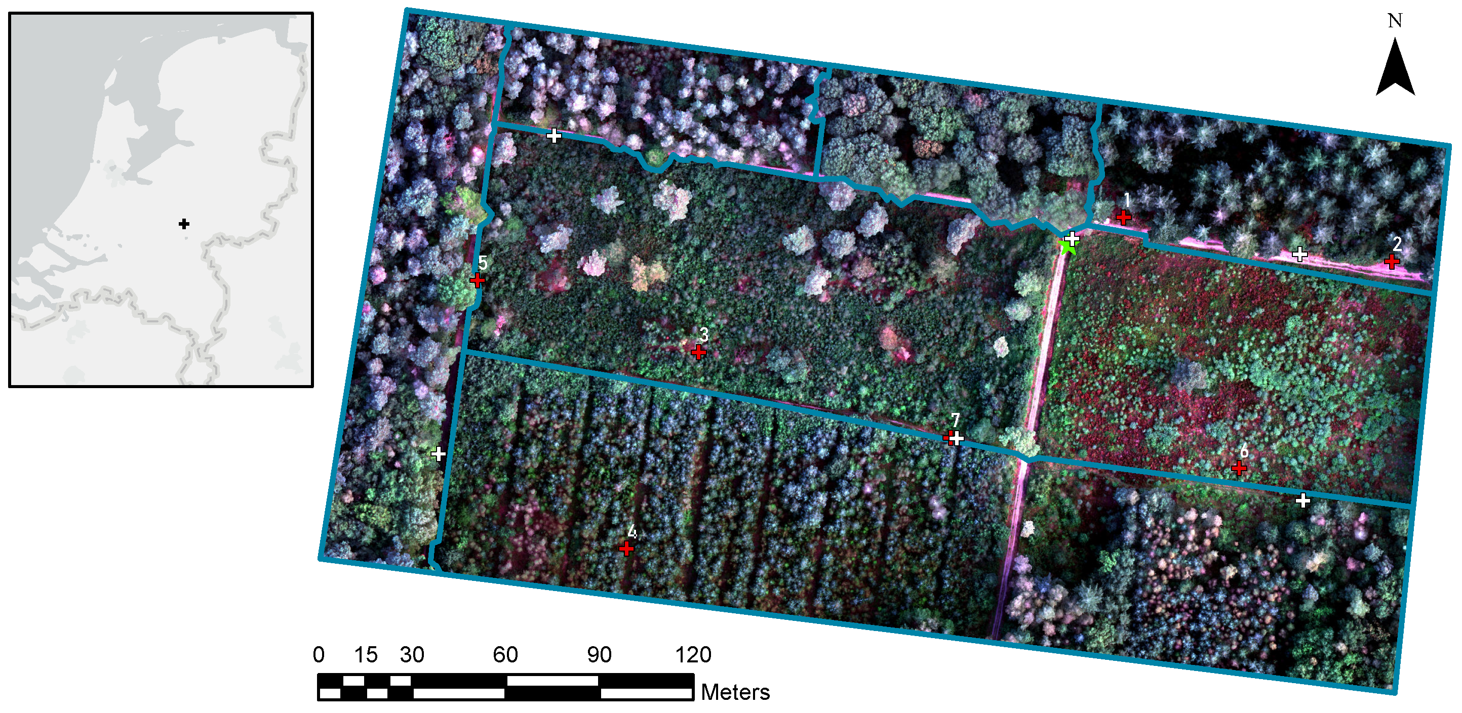
2.1. Study Area

A six-hectare forest northeast of Wageningen (51.993725 N, 5.718241 E) served as the area of interest. It lies between 40–51 m above sea level and can be considered largely flat. The area is subject to a maritime climate, with an average annual temperature of 10.6 °C and 848 mm of rainfall [55]. The area was selected due to its easy accessibility, clear visibility for UAV flights, and, most importantly, its variety of tree species. Comprised of both deciduous and evergreen tree species, as well as seedlings and mature vegetation, it represents a diverse ecosystem. The area can be divided into six areas: (1) the western part is a tree-dense mixture of deciduous and coniferous trees of varying heights (dense mixed); (2) the northwestern area contains predominantly conifer trees, mixed with some deciduous trees (coniferous mixed); (3) the mid-northern area only consists of deciduous trees (deciduous); (4) the northeastern part only has coniferous trees (coniferous); (5) the center area is covered with low-growing heath, shrubs, and some isolated deciduous and coniferous trees (sparse mixed); and (6) the southern part consists of small seedling coniferous and deciduous trees (small) (Figure 1). The dominant species in the area are the Scots pine (Pinus sylvestris), Douglas fir (Pseudotsuga menziesii), silver birch (Betula pendula), and American oak (Quercus rubra).

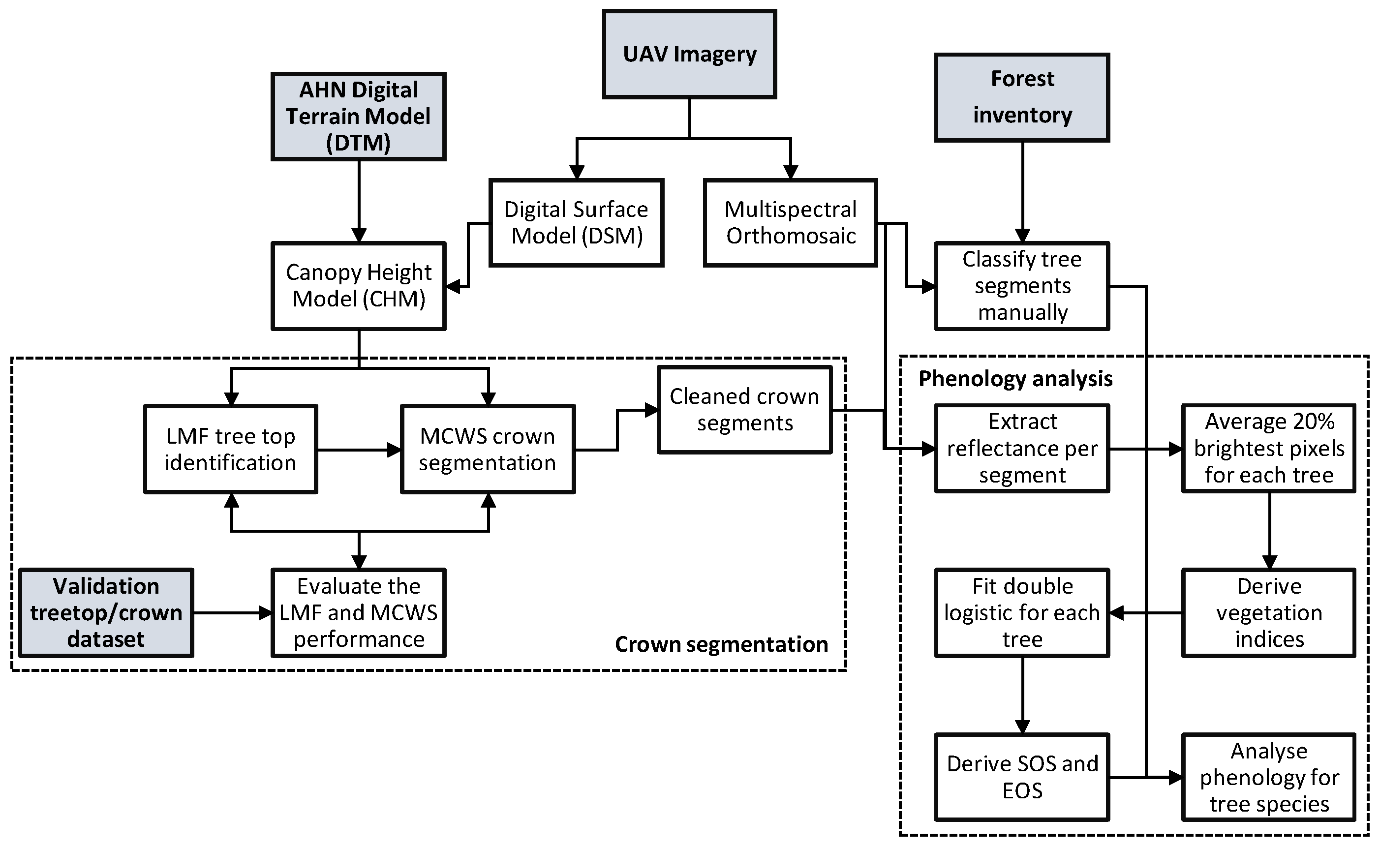
2.2. UAV Data Acquisition and Processing

In the period from 4 March to 12 December 2021, a total of fourteen flights were performed (Figure A1). At the beginning of the spring season, the flight frequency was roughly once every two weeks and increased to once per week during the peak spring season, decreasing to once a month during the summer and autumn. A DJI Matrice 210 quadcopter with real-time kinematic (RTK) GPS, in combination with a multi-spectral MicaSense Altum sensor was used. The Altum measures in five narrowband spectral regions: blue (475 nm, bandwidth = 20 nm), green (560 nm, bandwidth = 20 nm), red (668 nm, bandwidth = 10 nm), red-edge (717 nm, bandwidth = 10 nm), and NIR (840 nm, bandwidth = 40 nm).
Initially, the flights were performed in a preprogrammed grid at 60 m above ground level and with 80% frontal and lateral overlap, as recommended [56]. A sufficient overlap is required to ensure enough recognition points between the photos, to transform them into a single orthomosaic. However, the overlap between the images decreased during the spring season, as a result of the closing of tree canopies during budburst. Therefore, the last three flights were flown at 120 m altitude and in a dual grid.
Before and after each flight, a multi-spectral image was taken from a MicaSense calibration panel. UAV images capture the radiant flux at the sensor, which is dependent on weather and illumination conditions and, thus, hinders analysis over time and space [57]. With a calibration panel with a known reflectance, it is possible to account for the weather-induced differences in radiance between observations. Additionally, a sun sensor on top of the UAV measured the changes in radiance during the flight. The pre- and post-flight radiance values from the calibration panel combined with the in-flight sun-sensor values were used to convert the raw UAV images into surface reflectances. Taking into account the above-mentioned capabilities for accounting for fluctuating weather conditions, flights were conducted regardless of the illumination conditions.
During one flight on 26 July, six ground control points (GCPs) were placed, and their exact locations were measured using a Topcon RTK GPS pole. This flight functioned as the geometric reference and was used to geometrically correct all other flights.

2.2.1. Preprocessing

Radiometric calibration and structure from motion (SfM) procedures were performed within Agisoft Metashape software (v1.5.5) [58]. SfM uses recognition points in overlapping images and multi-view stereo (MVS) to stitch images together and estimate heights, enabling it to transform 2D images into 3D objects. SfM-MVS was used to create a dense 3D point cloud and a digital surface model (DSM), which were used as input to generate the orthomosaic (Figure 2). The key point limit (max number of points extracted per image) was set at 40,000, and the tie point limit (max number of alignment points per image) was set to 4000 (see full SfM settings: Figure A2). The 3D point cloud served as source data for the DSM, which represents the surface elevation. The orthomosaics from flights at 60 m had a ground sampling distance (GSD) of ∼2.5 cm/pixel compared to ∼5 cm/pixel for the flights at 120 m. Geometric correction was performed in ArcGIS Pro (v2.8.0) [59]. Achieving a high geometric accuracy is crucial for a spatial time series, to prevent shifting between the orthomosaics. A geometric correction based on the Topcon GPS measurements was performed on the geometric reference orthomosaic (on 26 July), to ensure an accurate global geometry. Relative to the corrected reference orthomosaic, the other orthomosaics were geometrically corrected using a first-order polynomial. Seven static objects in the study area served as GCPs, to ensure geometric accuracy between the orthomosaics (Figure 1). Due to the occasional occlusion of the GCPs, only five were selected for each correction. An average Euclidean error comparable to one GSD was obtained for all orthomosaics, corresponding to about ∼2 cm error for the low-altitude (60 m) flights and ∼4.5 cm at high-altitude (120 m) (Table A1).

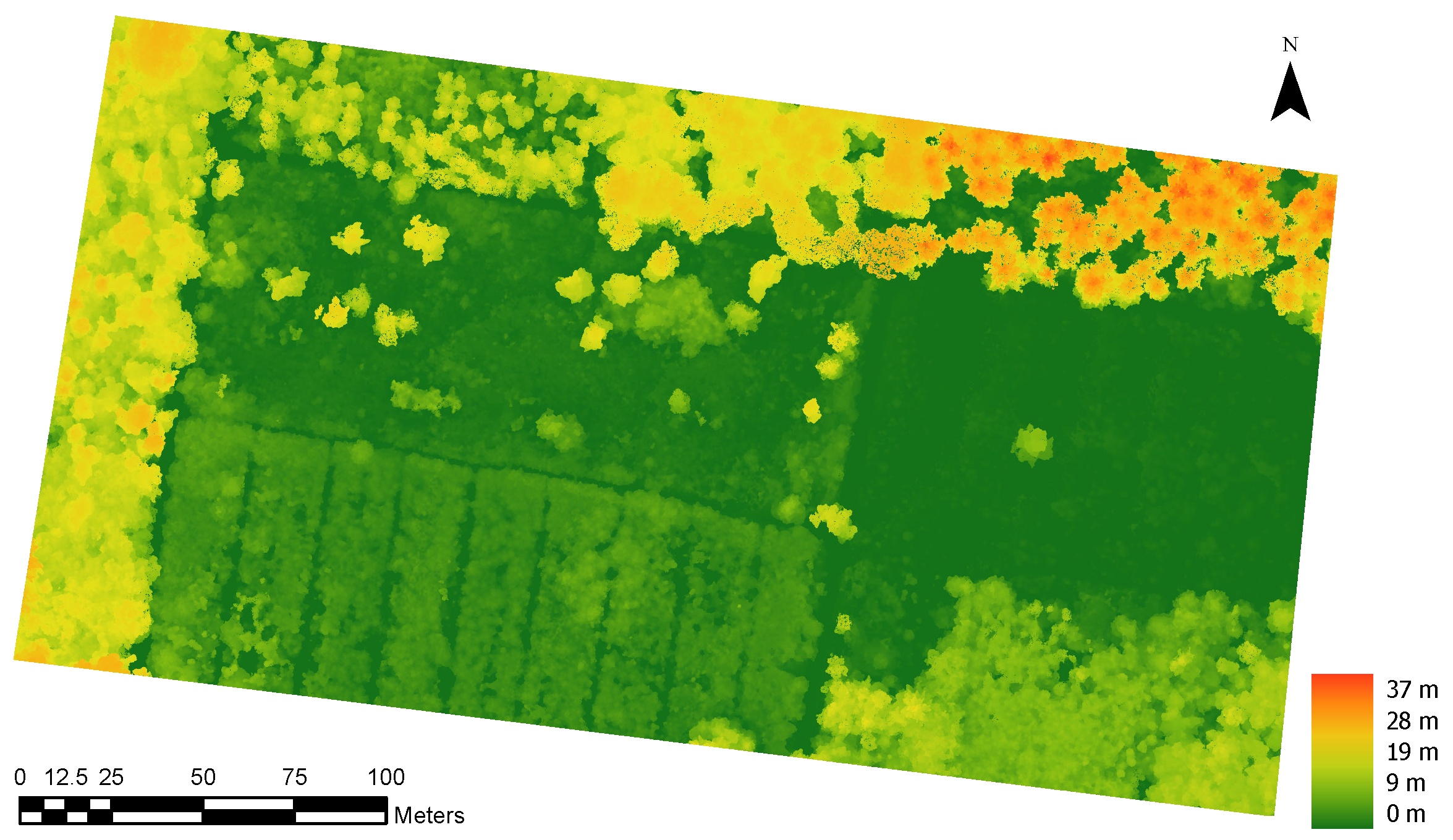
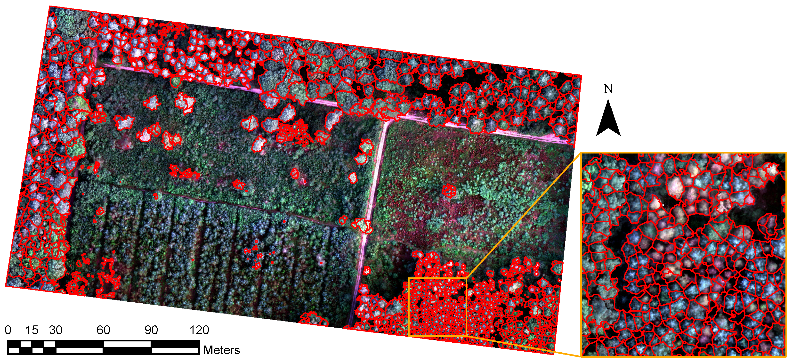
2.2.2. Automatic Tree Detection and Crown Delineation

Watershed segmentation is often performed with a canopy height model (CHM) [38,60,61]. CHMs emphasize the forest crown structure by subtracting the ground elevation, captured using a digital terrain model (DTM), from the surface elevation (DSM), making it appropriate for tree crown analyses. A clear UAV DSM with fully grown tree crowns is preferred for creating a CHM. The flight on 4 October best met these standards and was selected for the automated delineation. The DTM was acquired from the “Actueel Hoogtebestand Nederland” (AHN) (translated: “Current Height inventory the Netherlands”) [62]. This dataset uses light detection and ranging (LiDAR) to derive a DTM for the entirety of the Netherlands with a 0.5 m point density. Gaps in the DTM were interpolated with a focal mean filter with a 15 m window size. The interpolated LiDAR DTM was subtracted from the UAV DSM, to obtain the CHM (GSD ∼4.8 cm) of the study area. Due to discrepancies in the DTM and DSM, small negative values were present in the CHM, which were removed by coding them as 0. Lastly, a mean smoothing filter was applied to the CHM (window = 9 m), to alleviate noise in the raster and to make the height differences more distinct (Figure 3) [38,63]. Using the CHM, the tree crowns were automatically delineated, according to the following steps (see Figure A3 for schematic workflow):
Step 1: A local maximum filter (LMF) from the "lidR" package (v3.2.3) [64] was applied to the CHM, to detect the local peaks in the CHM raster. This technique creates a moving window around each pixel and codes a pixel as a treetop if it has the highest value in the window. A circular window was applied, as this is deemed more appropriate for detecting trees [65,66]. The window size is a crucial parameter, as a too-large window leads to errors of omission, due to unidentified trees, while a too-small window causes commission errors, where trees are counted multiple times. Traditional fixed window approaches struggle in diverse forests, due to largely varying crown sizes [38]. In response, Popescu (2004) developed a variable window that adjusts the window size based on the CHM value [66]. This method assumes a positive linear relation between tree height and crown size. In the case of multiple distinctively different homogeneous areas, multiple fixed window sizes can be appropriate. This study experimented with (1) a fixed window, (2) multiple fixed window sizes, and (3) a variable window size. For the multiple window approach, the area was split up into two strata, where one comprised the seedlings in the south (Figure 1), and the remaining area formed the other stratum. Different window parameter variations were examined, to find the optimal combination. This window optimization was performed iteratively by validating the results using various accuracy metrics, as described in Section 2.6. A mixed window size approach yielded the highest detection accuracy, which included a fixed window of W = 4 in the coniferous area and a variable window of W = 0.5 ( x 2 0.025 ) , where x denotes the tree height, in the rest of the study area. The hmin parameter, the minimum height at which a tree top is counted as such, was set to 8 m, based on a visual inspection of the CHM, in order to limit the number of detected trees. A total of 1371 treetops were identified.
Step 2: The delineation of the tree crowns was performed using the marker-controlled watershed segmentation (MCWS) within the "ForestTools" package (v0.2.5) [67]. The MCWS requires two input datasets, namely a raster representing the topography (CHM) and a point dataset with so-called “markers” representing the treetops. First, the CHM was inverted, to convert local maxima into local minima and vice versa. The inverted raster was then virtually filled, creating catchment basins. Where one basin touches another, a watershed line is drawn, representing the tree crown [38,45]. The markers prevent oversegmentation, as they only allow the creation of a basin when there is a marker, resulting in a one-to-one relationship between the predicted number of markers and tree crowns [68]. Additionally, the MCWS algorithm has a minimum tree height (MTH) parameter that sets the threshold, which must be lower than the minimum treetop height for a pixel to be considered part of a crown segment [67]. Setting this parameter high creates smaller segments and prevents non-tree-shaped segments but does lead to a lower overlap between the tree segment and the actual tree crown. Therefore, the segmentation accuracy was calculated for a range of MTH values, and the highest MTH value that retained an acceptable accuracy was selected. The segmentation accuracy assessment is explained in Section 2.6. Consequently, an MTH value of 7 m was found most appropriate, which resulted in 1944 segments. The number of segments exceeded the number of markers because the MTH value (7 m) was lower than the minimum treetop height (8 m).
Step 3: The resulting tree crown segments were cleaned, to make them better suited for further analysis. First, the segments without a corresponding marker were excluded from the dataset. Second, holes in the segments, due to foliage gaps or distortions in the CHM, were filled if smaller than 1 m2 using the filter in the “Smoothr2” package (v0.2.2) [69]. Subsequently, the crown edges were eroded, first, to account for geometric discrepancies between the orthomosaics and, second, to limit segments from covering multiple trees. A large erosion of 40 cm was applied. Last, crown segments smaller than 1 m2 were excluded. After cleaning, 876 segments remained.

2.3. Vegetation Indices

For each delineated crown segment, the multi-spectral pixel reflectances were extracted from each orthomosaic. Following Berra’s (2019) [21] approach, only the 20% brightest pixels in each crown in the green band were selected and used to compute the vegetation indices. This method limited the influence of both the understory and shading, as the brighter pixels prioritize sunlit pixels, which are more likely to be in the crown [21]. Furthermore, during leaf-off conditions, the brighter pixels tend to interact more with the tree branches and stems, which diminishes the influence of the understory and amplifies the seasonal signal. From the 20% brightest pixels, the mean reflectance for each spectral band was computed. The following vegetation indices were derived:
N D V I = N I R R N I R + R
E V I 2 = 2.5 ( N I R R N I R + 2.4 R + 1 )
O S A V I = ( 1 + 0.16 ) N I R R N I R + R + 0.16
C I r e = N I R R E 1

2.4. Field Reference Data and Manual Tree Classification

A field survey with a forestry expert was conducted in the study area, to collect ground truth tree species information. Various tree species were identified and geo-referenced. Based on the ground truth samples and a visual assessment of the orthomosaic time series, the 876 tree segments were classified manually. Some general tree characteristics were derived and used as a framework to classify the tree segments (Figure A5). Visual changes in vegetation over time were additionally used for the tree classification. Segments were excluded when the identification was not definitive, when a tree segment spanned over multiple crowns of different species, or when the segment included soil outside the tree crown. In case multiple segments covered one tree crown, their geometries were merged, to avoid an overestimation of the number of trees and to prevent a disproportional emphasis on smaller segments. Four deciduous and three coniferous species were identified in the study area (Figure A6). After the classification process, 273 segments were excluded, leaving 603 classified segments for the final analysis (Figure A7).

2.5. Fit Statistical Model

A statistical model was fitted to the vegetation index time series, to derive the phenological metrics [70]. Beck (2006) [71] proposed an improved logistic model capable of capturing both the green-up and senescence phase, by adding two parameters to the traditional logistic model. It was found that a double logistic model captures the seasonal phenology better compared to other models, such as a Fourier series or an asymmetric Gaussian function [71]. Mathematically, the double logistic model is described as follows [71]:
V I ( t ) = V I w + ( V I m V I w ) 1 1 + e m S ( t S ) + 1 1 + e m A ( t A ) 1
where VI is modeled as a function of time (t). This function estimates six parameters, namely the VI during winter ( V I w ), the maximum VI value ( V I m ), the two inflexion points where the curve rises (S) and declines (A), and the rate of change at the two inflexion points ( m S and m A ). The estimated inflexion points, S and A, represent the SOS and EOS dates, respectively. The “greenbrown” package (v2.5.0) in R was utilized to fit Beck’s double logistic model to the VI time series [72].
Estimation of the logistic parameters is based on the maximum likelihood and is thus an iterative process [73]. The number of iterations determines the goodness of fit of the ultimate convergent curve. The root mean squared error (RMSE) (Equation (6)) was computed under various iterations for ten randomly selected trees (Figure A8). Based on these results, the iteration parameter was set to 300.

Evaluate Model Performance

The root mean squared error (RMSE) is not an ideal metric for a double logistic fit. A curve with small residuals does not automatically describe the tree phenology well, since the shape of the curve and the accuracy of the inflexion points are not captured in the RMSE. Nevertheless, the RMSE does give some indication of the goodness of the fit and was therefore used as one of the metrics to assess the model quality. A normalized RMSE was used, which controls for the VI unit by dividing by the mean. This was determined with the following equations:
R M S E = 1 n Σ i = 1 n y i y ^ 2
n R M S E = R M S E y ^

2.6. Validation of the Crown Delineation

A treetop and crown validation dataset was created, to assess the quality of the automatic crown delineation and to optimize the ultimate tree segmentation. From a subset of trees, the tops were manually identified and their crowns were manually delineated based on the orthomosaic of 4 October (Figure A4). Due to the diversity in tree type, species, height, and distribution in the study area, a stratified sampling design was selected. Stratification divides the study area into distinct homogeneous areas and allows assessing the segmentation performance in different types of vegetation structures. A validation dataset was created in ArcGIS Pro (v2.8.0) [59]. First, the area was divided into six sections (Figure 1) and a random point was generated in each section. Subsequently, a 25 m square buffer was created around each point, except for the southern area, where a 15 m buffer was deemed sufficient. Tree crowns that fell within these validation plots for more than 50% were included in the validation dataset. Similar to the automatic delineation, only treetops above 8 m and tree crowns above 7 m were included. A total of 134 treetops and crowns were manually digitized.
  • Tree identification
The true positives (TP), false positives (FP), and false negatives (FN) of the LMF tree identification were determined based on the validation data. In case multiple treetops were identified in one reference crown, the highest treetop was coded as TP and the others as FP. The LMF treetop was also coded as FP when predicted to be outside of a tree crown but inside the validation plot. A reference crown without a corresponding treetop was counted as FN. Consequently, the LMF performance was expressed using the following metrics:
R e c a l l = T P T P + F N
P r e c i s i o n = T P T P + F P
F s c o r e = 2 p r e c i s i o n r e c a l l p r e c i s i o n + r e c a l l
  • Tree crown segmentation
The automatic delineation performance was assessed by comparing the segmented tree crowns (S) with the reference tree crowns (R). Tree crown segmentation strives to represent an individual crown using a single segment. Accordingly, the quality of the segmentation is not only based on the size and location of the segment but also on its shape, making the accuracy assessment different to traditional binary classification assessment [38]. As we are interested in the one-to-one accuracy of the predicted segment, only the true positives were used. In case multiple segments were delineated in one reference crown, the segment with the highest treetop was selected.
The oversegmentation (OS) and undersegmentation index (US) indicate the proportion of overlap between S and R in relation to the total area of either S (US) or R (OS) [74]. They are defined using the following equations:
O S = 1 | R i S i | | R i |
U S = 1 | R i S i | | S i |
where | R i S i | is the intersection of the reference (R) and segmented (S) and denotes the overlapping area between the two. When OS > US, this indicates oversegmentation, whereas there is undersegmentation when OS < US. An OS and US of 0 indicate a perfect match between the reference and segmented tree crown, whereas a value close to 1 indicates almost complete dissimilarity. The intersection over union index (IoU), also called the Jaccard index, provides the ratio between the area of overlap of two segments and their combined area [75]. Mathematically, the equation is written as follows:
I o U = | R i S i | | R i S i |
where | R i S i | denotes the area of the unionized geometries of R and S. This ranges from 0 to 1, with 0 indicating no overlap at all and 1 representing perfect similarity. The advantage of the IoU index is that the overlap is a function of the total combined area and thus provides an appropriate picture of the similarity of R and S relative to their size.

3. Results

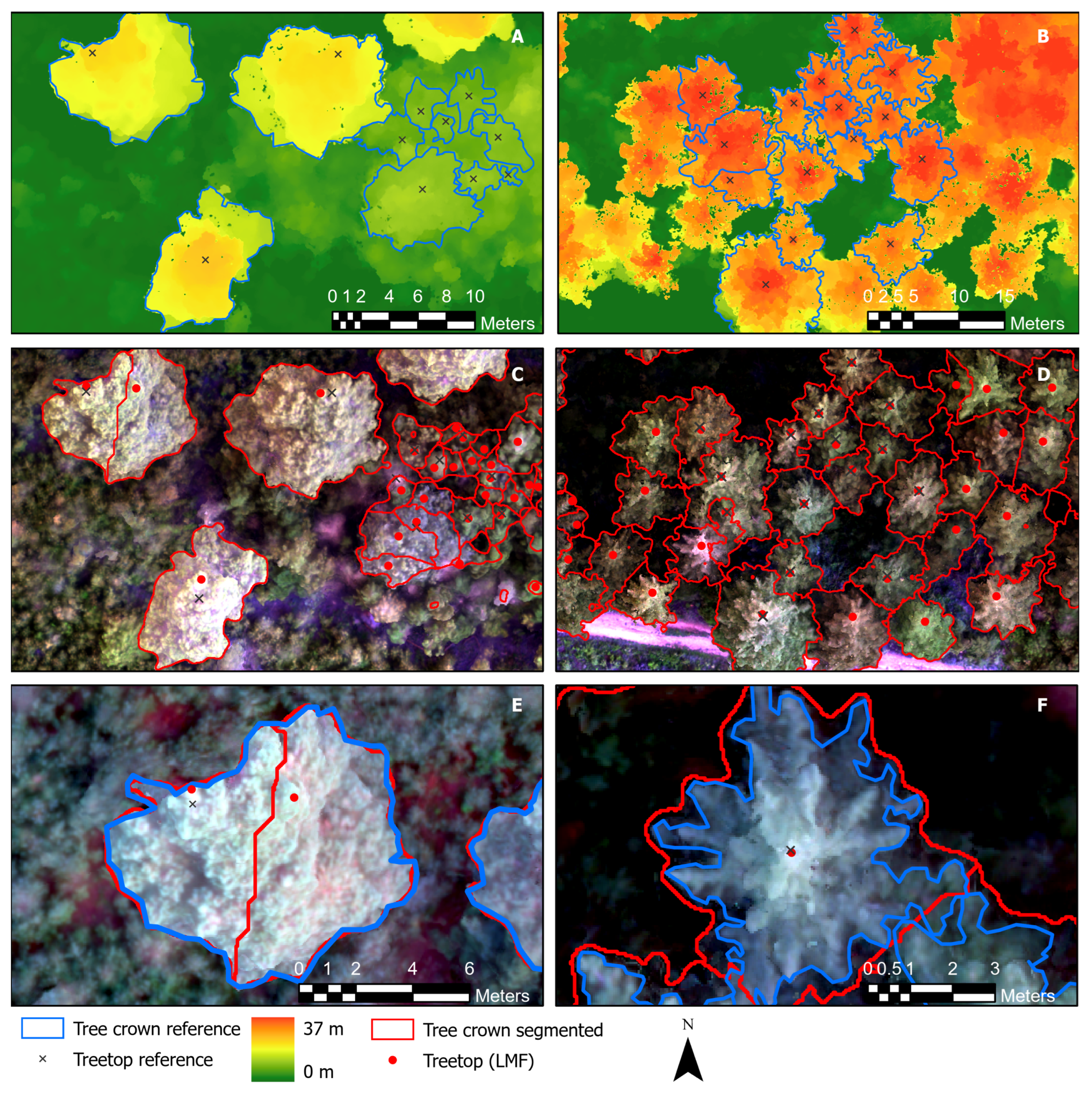
3.1. Automatic Crown Delineation

The LMF tree detection produced an average recall and precision of 0.78 and 0.81, respectively (Table 1). These results indicated that the LMF detected 78% of the actual reference trees and that 81% of the trees detected were correct. However, there were substantial variations in performance related to the different types of vegetation in the area. Coniferous trees appeared to be easily detectable, based on high F-scores (coniferous: 1, coniferous mixed: 0.95) (Table 1). Additionally, the LMF tree detection performed well on deciduous trees, with an F-score of 0.92. Lower accuracies were observed for small trees (F-score: 0.73) and in areas with more heterogeneity (dense mixed: 0.66, sparse mixed: 0.65). In the small and dense mixed area, the primary source of error came from omission errors, as the precision exceeded the recall. Errors of commission were most prominent in the sparse mixed area.
The tree crown segmentation result can be found in Figure 4. The overall accuracy was indicated by the IoU and implied an overlap of 58% between the segmented crown (S) and the reference crown (R) in relation to their combined area (Table 1). The MCWS tended to undersegment, as indicated by the US (0.34) exceeding the OS (0.15). This shows that, on average, the area outside the overlap was larger for S than for R. Additionally, the low OS indicated that a large part of a reference crown was covered by a single segmented crown. The segmentation performance was highest in areas dominated by coniferous vegetation, with an IoU of 0.71 and 0.65 in the coniferous mixed and coniferous areas, respectively. In particular, the OS was low in these coniferous areas (0.08 and 0.13). Oversegmentation was dominant in the sparse mixed area (OS: 0.34 > US: 0.16). The lowest segmentation accuracy was achieved in the small and dense mixed areas, with an average IoU of 0.45 and 0.41, respectively. In both these areas, the US was particularly high, implying that large parts of S fell outside R.

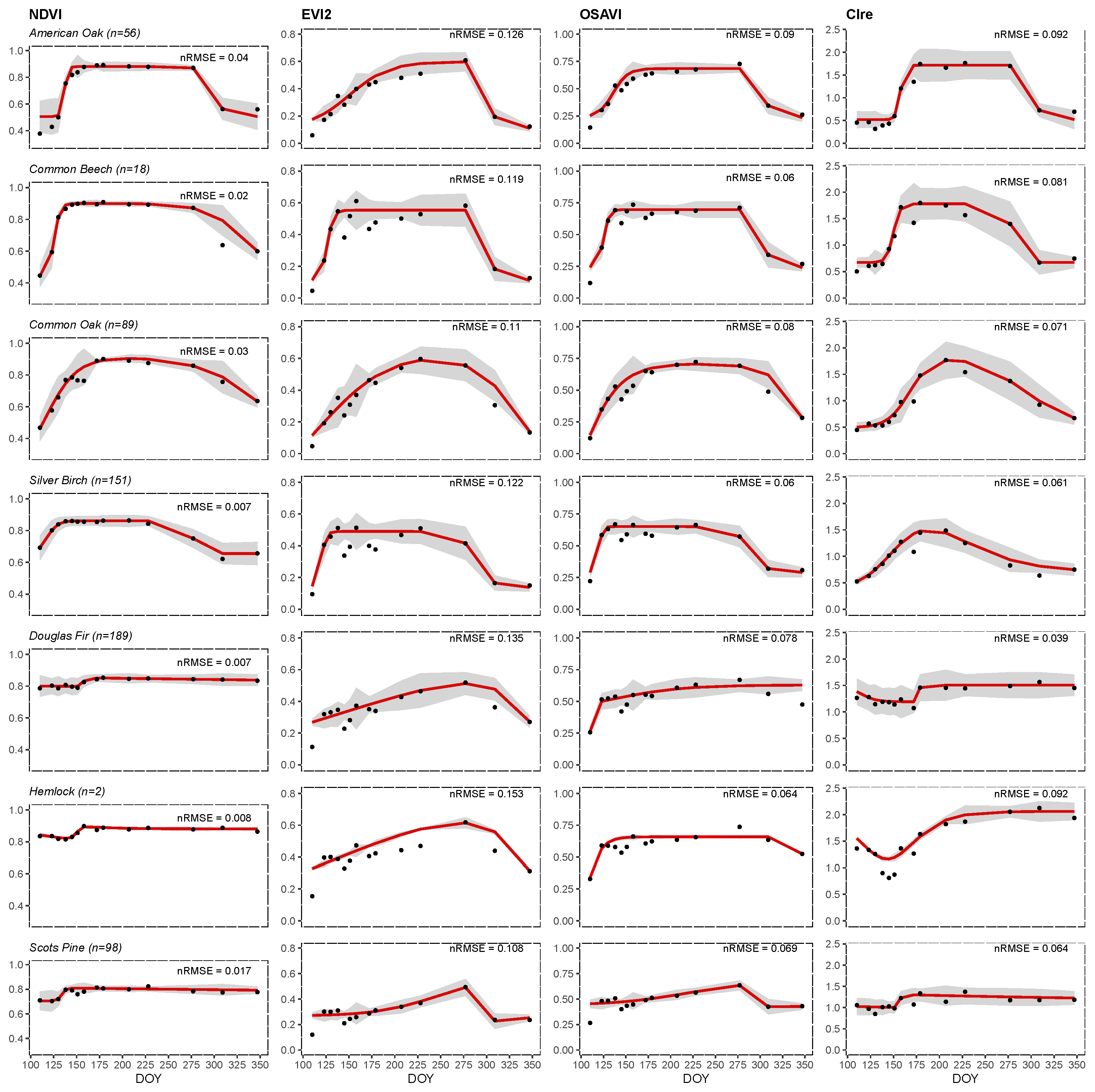
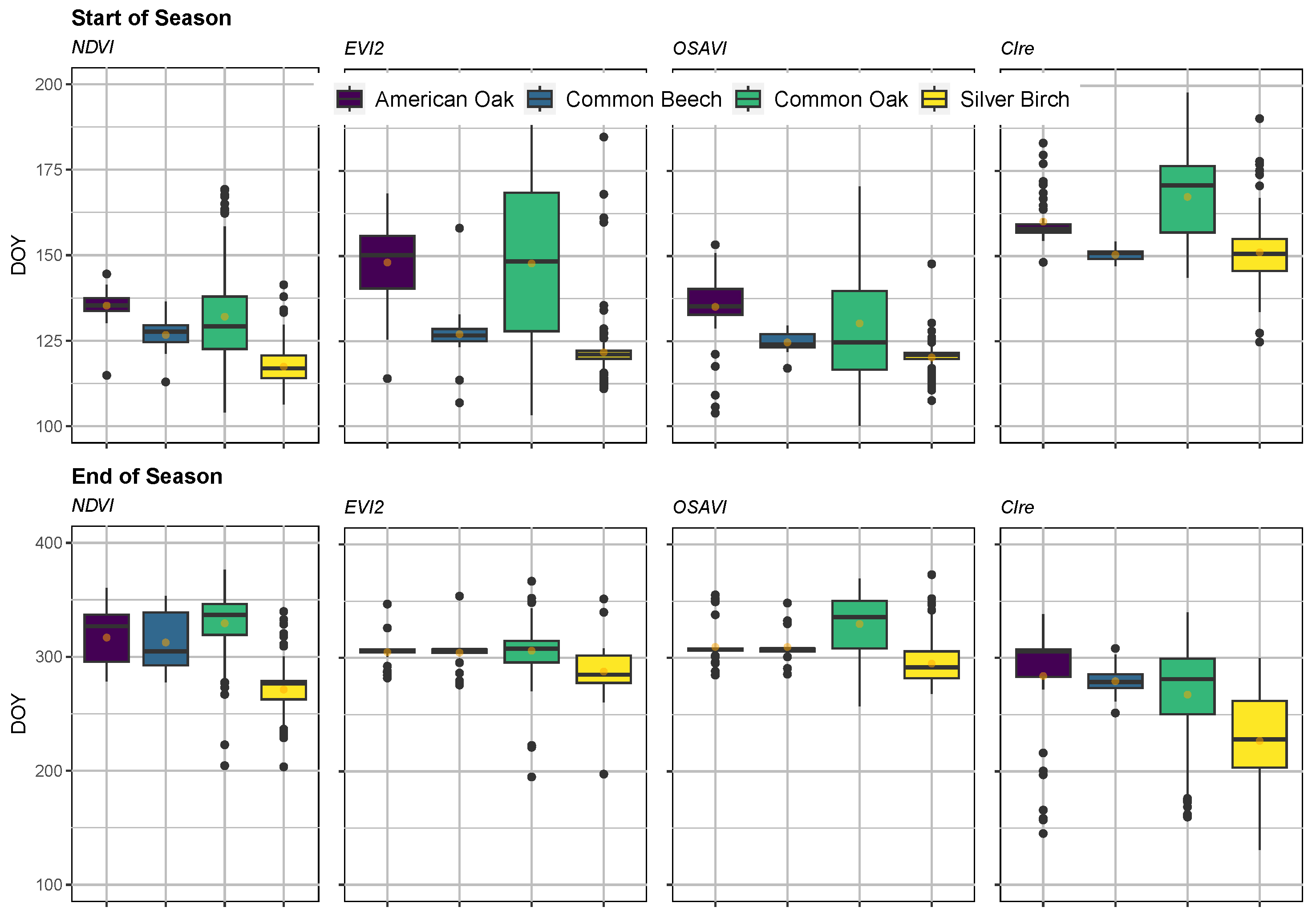
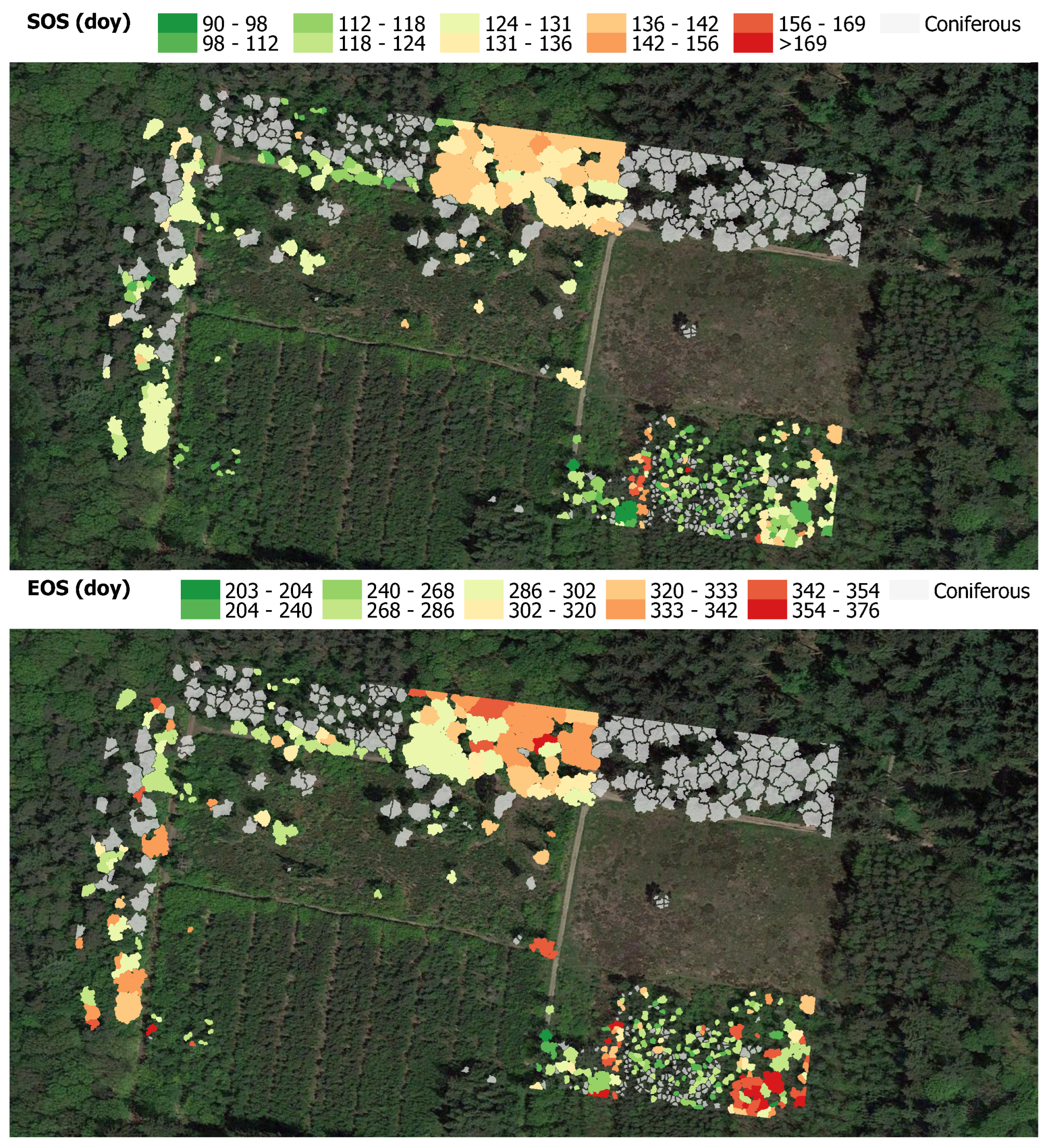
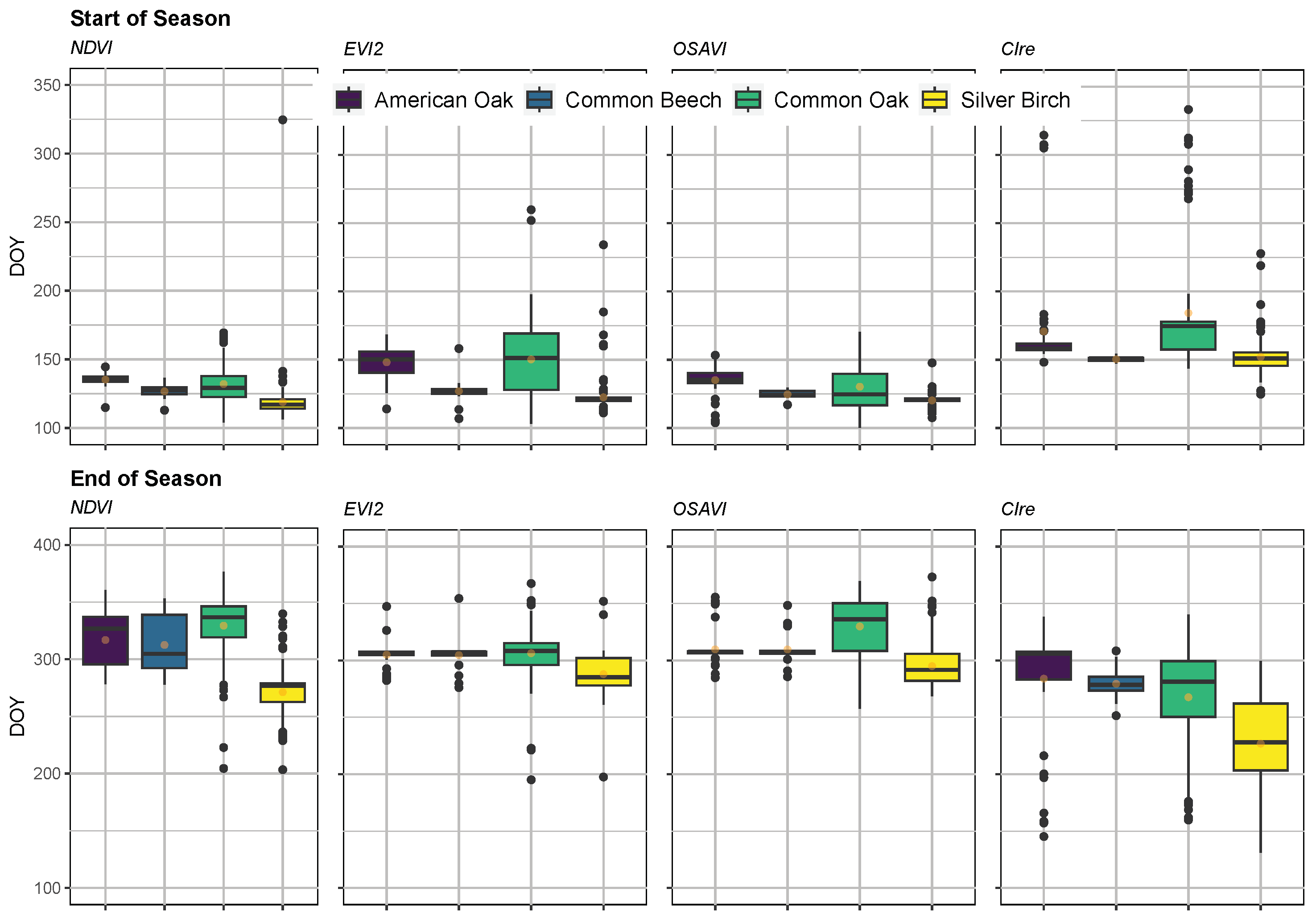
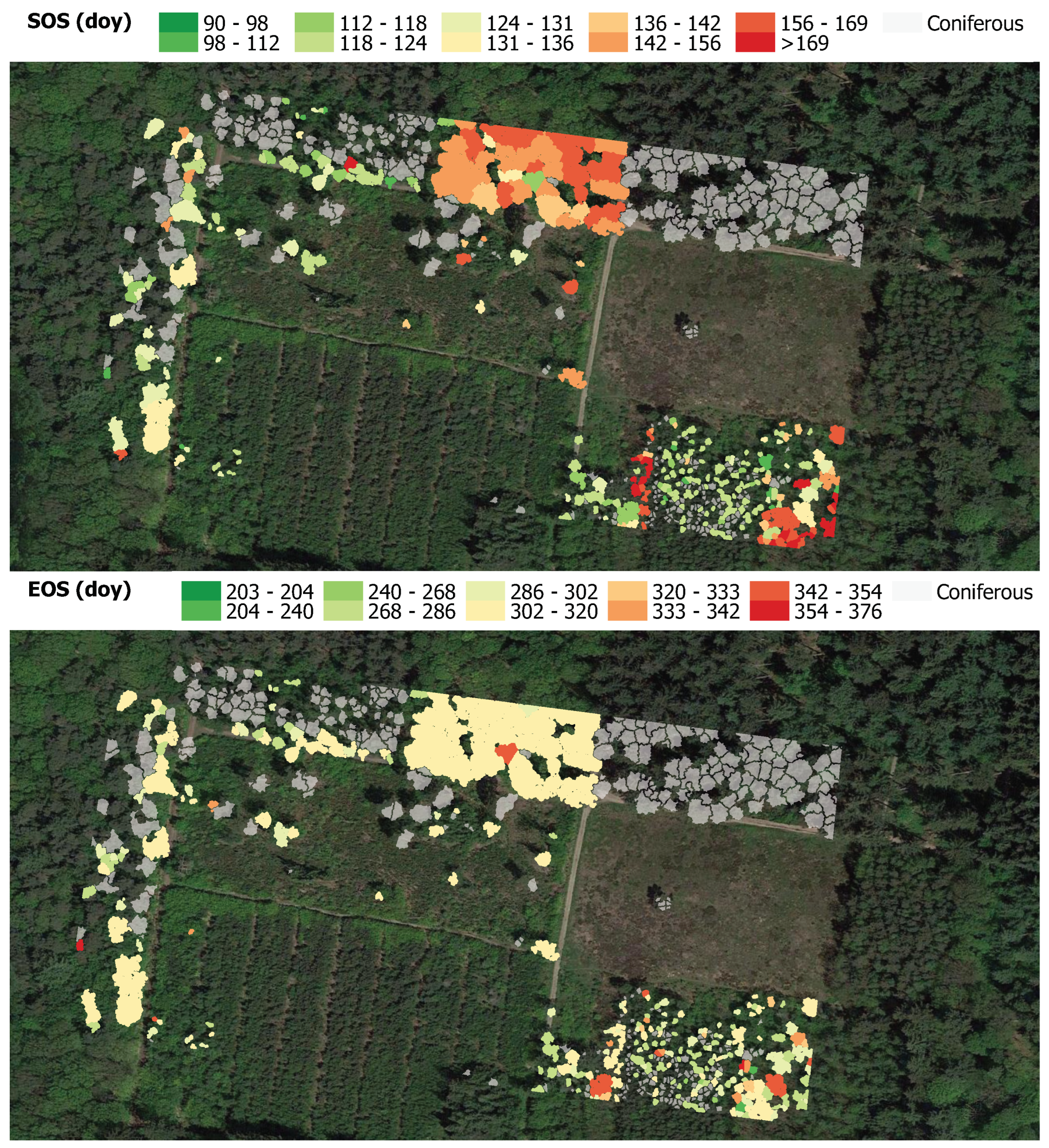
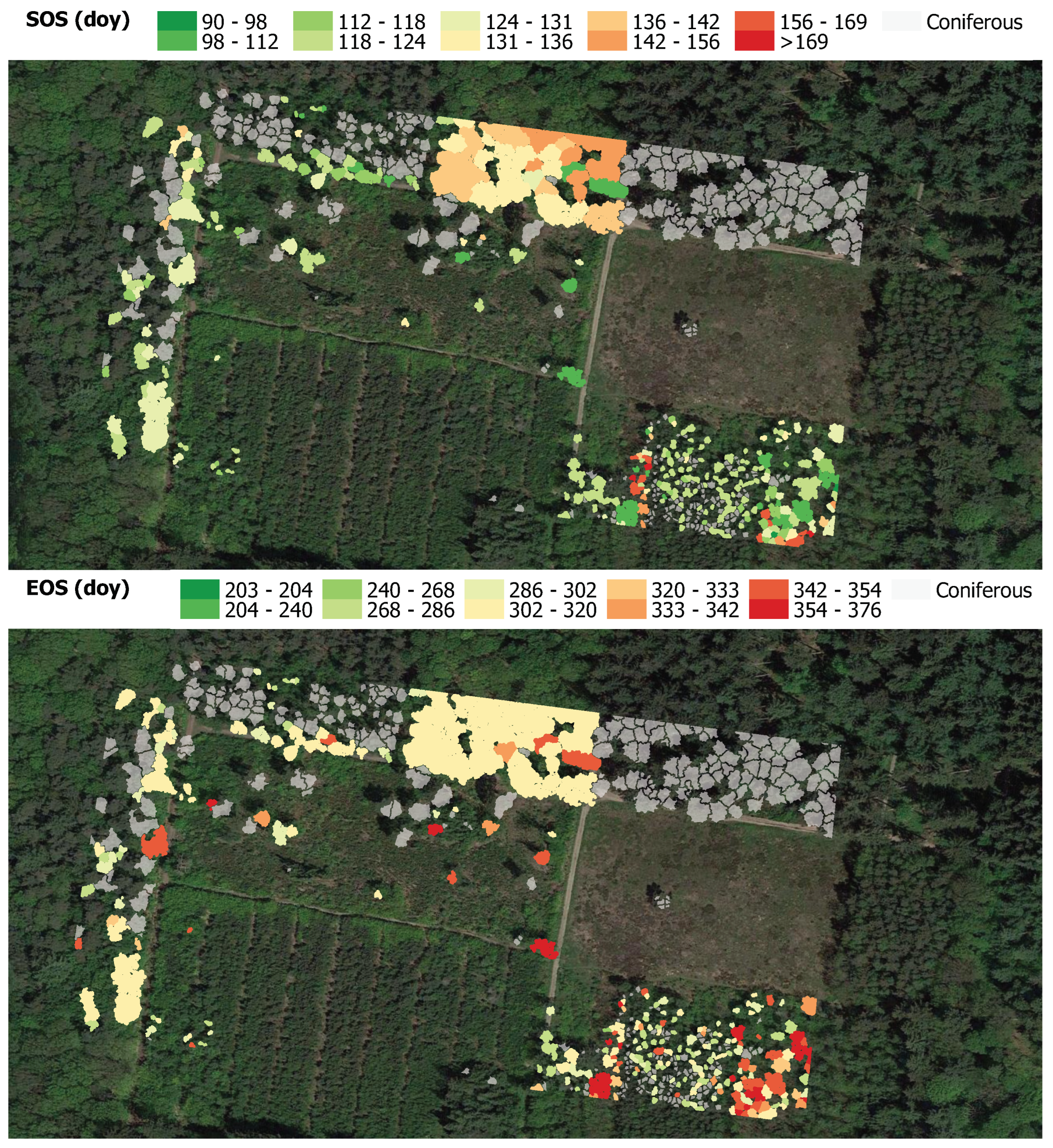
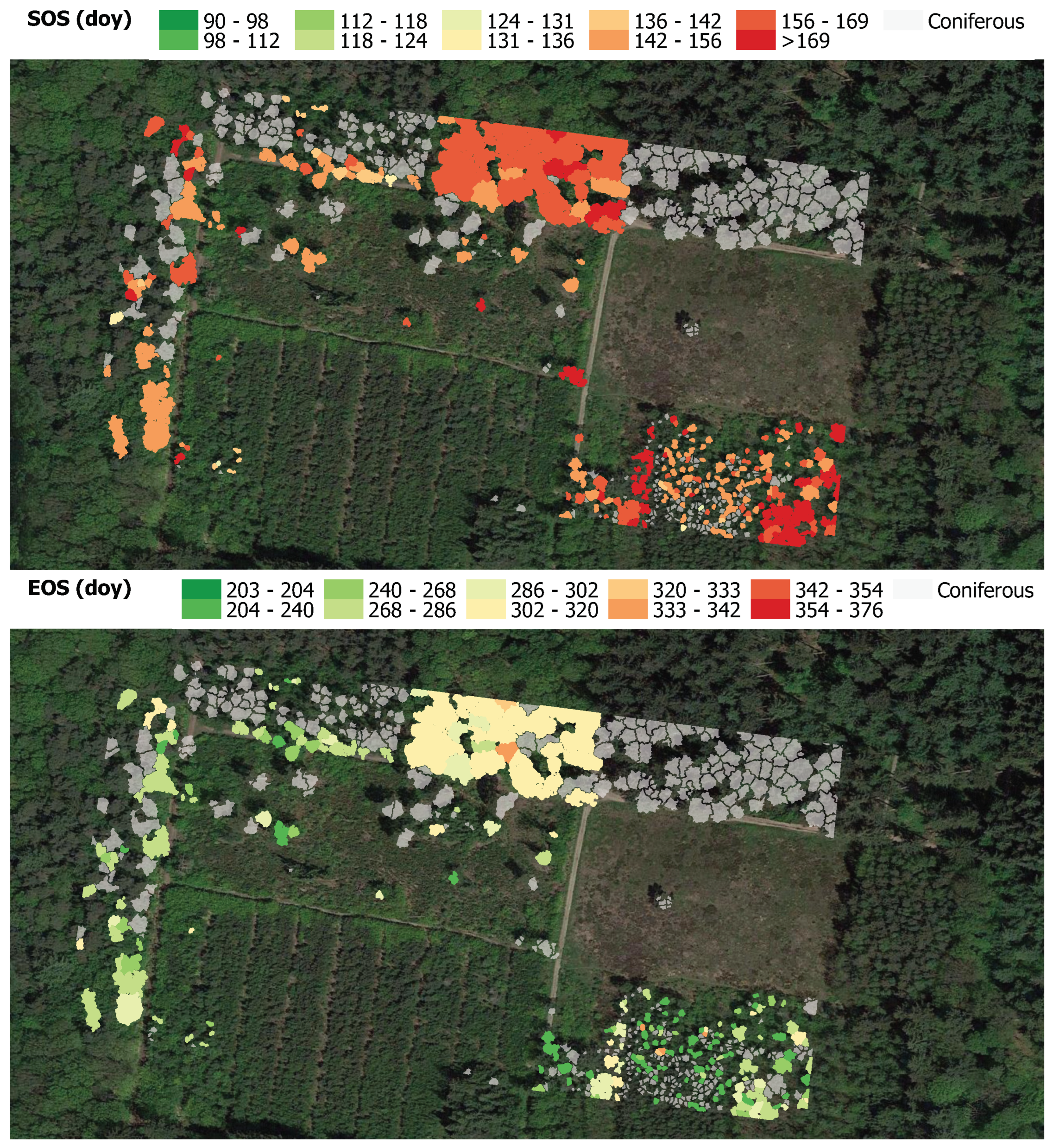
3.2. Phenology Monitoring

For the deciduous tree species (American oak, common beech, common oak, and silver birch), the average VI values over time, based on the 20% brightest pixels, showed clear variation and portrayed a phenological trend consistent with the expected budburst and senescence (Figure 5). The left side of the double logistic curve represents the average species VI value during wintertime, followed by an increase during spring onset, a maximum during summer and, lastly, a decrease in the VI indicating the tree senescence. Some of the VI time series contain outliers, as is the case for silver birch and common beech (Figure 5). However, these distortions seem to affect the ratio-based NDVI, and to a lesser extent the CIre, less than the EVI2 and OSAVI. Overall, the NDVI appears robust, with few outliers, resulting in a low nRMSE ranging between 0.006 and 0.049. On the contrary, the model fitted on the EVI2 showcased the highest nRMSE (0.13–0.148).
The NDVI displays a clear plateauing effect due to saturation, which is less the case for the EVI2. This indicates that the EVI2 captured more variance over time and may include phenology characteristics missed by the NDVI. Similarly, the CIre also captured much of the seasonal variation and has a lower nRMSE than the EVI2 (Figure 5). For the CIre, EVI2, and OSAVI, the spread in observations tended to be lower during the spring and autumn, and higher during summer (Figure 5). The NDVI displayed generally less spread during the summer, which was likely due to saturation. On a species level, the lowest spread was observed for the common beech, followed by silver birch, with the highest for the common oak. Beech trees had a steep VI increase in spring, indicating a uniform species-wide green-up period (Figure 5). The common oak displayed more within-species variation, which is represented in the large spread in the phenology estimates (Figure 6). Moreover, the common oak had a late budburst and senescence. Of the deciduous trees, the silver birch showed the earliest spring onset (DOY 118-122), as well as the earliest EOS (DOY 271-295), excluding the CIre-derived estimates (Table 2). Notably, the CIre consistently modeled a later onset and earlier senescence compared to the other VIs (Figure 6). Spatially, trees with similar SOS estimates tended to cluster together, while there was more spatial heterogeneity in the EOS estimates (Figure 7). In the western area, many trees > 7 m were missed, as the crown polygons were deemed too poor and excluded during the classification process (Figure A7). The spatial display of the SOS and EOS estimates, derived from the EVI2, OSAVI, and CIre can be found in Figure A10, Figure A11 and Figure A12.
Limited phenological variation was observed for the coniferous tree species (Douglas fir, hemlock and Scots pine). This is exemplified by the almost linear double logistic fit of the ratio-based indices (NDVI and CIre) (Figure 5). The EVI2 and OSAVI captured a slight coniferous seasonality. However, these two VIs displayed a different pattern for the Douglas fir; moreover, for the Scots pine, their curves seemed to be pulled by a single observation at DOY 277. Correspondingly, the average SOS and EOS for the coniferous species are accompanied by large standard deviations (Table 2). Due to this lack of seasonal variation in coniferous phenology captured by the VIs, and the subsequent unreliable SOS and EOS estimates, the coniferous SOS and EOS estimates have been left out of Figure 6 and Figure 7.

4. Discussion

4.1. Explaining the Vegetation Index Trends

The VIs captured a clear seasonal signal for the deciduous tree species over time. However, for the coniferous species, marginal VI variation was observed. Consequently, the phenological meaning of the metrics for the coniferous trees is questionable, as seasonal variation is required to fit a meaningful double logistic curve. This is in line with previous studies that found structural VIs captured almost no variation for evergreen species [21,26,31,50,51]. Structural greenness indicators rely on visible changes in greenness as a vegetation proxy [76] and, therefore, function well for deciduous trees whose phenological transitions rely on morphological changes [19,77]. Physiological indices capture biochemical changes better and have been found to outperform structural indices when monitoring evergreen phenology [50]. Nevertheless, in this study, the physiological chlorophyll-sensitive CIre [78,79,80] also detected no seasonal variation for coniferous species. This is likely due to evergreen conifers retaining most of their chlorophyll in their needles throughout the year, hence showing little seasonal variation in chlorophyll [81]. Carotenoid-sensitive VIs, such as the photochemical reflectance index (PRI) or the chlorophyll/carotenoid index (CCI), were found to better capture seasonal variation in evergreen species [51].
Previous studies found consistent early SOS predictions for structural VIs linked to the early greening of the understory [82,83]. Soil-sensitive indices such as the NDVI were found to be more susceptible to this understory effect compared to soil-adjusting indices such as the EVI2 and OSAVI [50,84]. In this study, the NDVI-derived SOS for the deciduous trees was predicted earlier (DOY 118–135) than the EVI2-derived estimates (122–150), but the NDVI-derived SOS was comparable to the OSAVI-derived predictions (120–135). The similar NDVI and OSAVI SOS estimates seem to contradict the influence of the understory on the soil-sensitive NDVI. However, in this study, a considerable part of the background influence was mitigated by only using the brightest 20% of pixels [21]. This background mitigation might have especially benefited a soil-sensitive index such as the NDVI. Furthermore, the late SOS estimates for the EVI2 are noteworthy, especially for the American and common oak (Figure 6). While the exact reason for this is unknown, the late saturation of the EVI2 compared to the NDVI and OSAVI [85,86] could provide an explanation. For a quick-growing species such as beech or birch, the higher EVI2 saturation would not cause a large SOS difference, but for species that grow more slowly, such as the oak, this could explain the significantly later SOS. The high saturation level might also explain the EVI2’s relatively high standard deviation during summer (Figure 5), as it captures a wider range of vegetation levels relative to the other VIs. Accordingly, this study detected minimal NDVI variation in summer, in line with existing literature reports [31,51].
Another remarkable result was the consistently late SOS estimates derived from the CIre (Figure 6). Deciduous trees display a morphological change of leaf growth in spring, prior to the accumulation of pigments (e.g., chlorophyll) in summer [19,77]. As the increase in greenness occurs prior to the increase in chlorophyll, a later increase in the chlorophyll-sensitive CIre, and the corresponding SOS date, is expected. This is also in line with previous observations from Kikuzawa (2003) [87] and Dong (2015) [78]. Furthermore, EOS dates were estimated consistently later by structural indices compared to ground truth observations [50,83,88]. Late EOS estimates are often observed, as photosynthesis in deciduous trees is governed by photoperiod, whereas autumn leaf-fall is a function of temperature, causing the photosynthesis to end prior to the structural recession [83,89]. Since temperatures in the autumn of 2021 were above average [55], late EOS estimates from structural indices were expected. Hence, significant differences between the structural VI EOS estimates (DOY 305–330) and the CIre EOS estimates (DOY 227–284) were found.

4.2. Tree Phenology Estimates in Context

The ongoing citizen science project called “The Nature Calendar” (Dutch: “de Natuurkalender”) contains information on the date of first leaf development (comparable to SOS) and leaf-off dates (comparable to EOS) [90]. Yet, the phenology observations from the nature calendar, used as reference, are based on structural changes of trees and will therefore inherently deviate from physiological CIre estimates. Therefore, for the sake of providing a meaningful comparison, the CIre was excluded when comparing absolute SOS and EOS dates.
The silver birch displayed the earliest average SOS between DOY 118 and 122 (Table 2). Its estimates showed little spread, and the marginal within-species variation indicates a uniform budburst. A similar uniform budburst was observed for the common beech, but with a later average SOS (DOY 124–127). Correspondingly, ground observations in the area of Wageningen confirmed the earlier development of leaves for the silver birch [90]. Similarly, other UAV-based phenology studies observed minimal within-species SOS variation for beech, consistent with this study’s findings [31,32]. Moreover, while there is not much information on the EOS of the birch in the nature calendar, it does give an earlier autumn foliage condition for the birch compared to other deciduous species [90], which was also found in another study performed in Japan [32]. Furthermore, previous analyses consistently modeled large phenological within-species variations for oaks [21,31,51,91], which correspond with this study, particularly for the common oak. Some NDVI-based studies estimated oak SOS around DOY 130–132 [21,31,51] and oak EOS between DOY 274 and 300 [51,91]. This corresponds well with the NDVI-derived SOS estimates of DOY 130–135 found in this study but less well with the EOS estimates of 317–329 (Table 2). High temperatures during the autumn of 2021 could account for the late oak EOS. Lastly, the ground observations from the nature calendar, as well as various satellite-based phenology studies, support the findings of a generally late budburst and late senescence for oak trees [90,92,93,94].

4.3. Evaluating the Automatic Tree Crown Delineation

This study found an overall recall, precision, and F-score of 0.78, 0.81, and 0.79, respectively, with considerable performance differences between the various forest types. Tree detection accuracies were highest for areas with coniferous (F-score: 0.95–1.00) and deciduous trees (F-score: 0.92), and lowest for mixed tree patches (F-score: 0.65–0.73) (Table 1). These results exceeded the detection accuracies of some UAV-derived tree segmentation studies, which achieved an overall accuracy of 67% [95] and 63% [21]. This is comparable to more recent studies from Xu (2020) [96] (overall F-score: 0.83%) and Belcore (2020) [97], who realized an F-score of 0.73 in coniferous Alpine tree detection using a Hölder exponent. Forest structure is detrimental to the quality of the tree detection result. For instance, very high accuracies, exceeding 95%, were achieved when considering coniferous monocultures [98], while complex mixed forests are far more challenging for automatic tree detection [99]. This was reiterated by Berra (2019) [21], who achieved a significantly higher detection accuracy for coniferous trees (recall: 0.73–0.80, precision: 0.78–0.82) compared to for deciduous species (recall: 0.43–0.57, precision: 0.43–0.63). The conical shape of coniferous trees allows for an accurate detection, due to the distinct height difference and the relatively large distance to other treetops, as is visible in Figure 8B,D. Mixed deciduous forests, on the contrary, are characterized by overlapping crowns and less distinct treetops (Figure 8A,C). The issue of varying crown sizes was partially addressed in this study by using a variable window size for the LMF. Other factors such as the segmentation method, illumination conditions, and quality of reference data influence the tree detection accuracy as well, stressing the need for careful interpretation when comparing results [97]. Nevertheless, the detection accuracy achieved in this study appears to be on the high end compared to the existing literature. The window size optimization might have been an important factor in the high detection accuracy achieved.
Generally, the average US (0.34) exceeded the average OS (0.15), indicating that the segmented crowns were typically larger than the reference crowns, called undersegmentation. MCWS tends to undersegment, as the watershed ridges inherently grow until they encounter another ridge, making the method prone to including areas outside of the actual crown. Actual tree crowns are not always connected as seamlessly as is assumed by the MCWS, leading to this discrepancy. In the sparse dense stratum, however, the OS (0.34) was larger than the US (0.16). Here, due to the low tree detection precision (0.48), there were many false positives, resulting in segmented crowns that were too small, causing the high OS (see example in Figure 8C,E). Furthermore, the IoU of the deciduous trees (0.64) was comparable to the coniferous result, which is striking given the more complex crown structure of deciduous foliage. Belcore (2020) [97] performed a multi-resolution tree segmentation in a coniferous Alpine forest and achieved an average IoU of 0.72. Although this is higher than the average IoU achieved in this study (0.58), it is only slightly higher than the IoU scores found in this study’s coniferous tree strata (0.65 and 0.71).

4.4. Considerations for Future Research

After geometric corrections, this study achieved a relative Euclidean error of around one GSD, comparable to other studies [31]. This shows that dedicated GCP placement is not necessarily required when only relative geometric alignment is needed. Nevertheless, placing in situ RTK-measured GCPs is still the norm in UAV multi-temporal analyses [21,31,100]. Additionally, it is worth noting that the geometric error is measured at ground level and is likely to increase higher up in the canopy, due to the flexible nature of trees. This was addressed in this study by eroding the segmented crowns by 40 cm, to minimize the influence of the neighboring crowns, even when some geometric variation over time occurs. However, due to the occasional poor alignment of the images during the structure from motion process, there were sporadic geometric distortions at the edge of the orthomosaics, which compromised the geometric accuracy. During the manual classification, these distortions were identified, and the affected crown segments were excluded if too severe. Notably, this warping at the edges only occurred for the flights performed at 60 m altitude and not when flying at 120 m. Due to the closing up of the foliage during spring, the overlap between the images decreased over time. Consequently, for the flights at 60 m, the SfM could not align all images, which, ultimately, resulted in a smaller orthomosaic area size, with some geometric distortions at the edges. Therefore, in future studies, higher-altitude flights, at the expense of spatial detail, would be preferred, to prevent such geometric distortions and allow for a larger UAV coverage.
Furthermore, the frequency of the observations is important for the double logistic fit, as sufficient data points are needed to determine a well-characterized winter baseline. In this study, the first flight was performed on 20 April (DOY 110), at which point some early-growing silver birches were already developing leaves. Hence, in some cases, the time series did not capture the complete leaf-off situation, which may have caused the inflexion point to shift and led to occasional erroneous fits. Another consideration is the uneven distribution of the flights (Figure A1). While flights were performed frequently during spring, only a limited number were executed in the autumn. While a higher number of observations is generally preferred, previous studies indicated that accurate phenology estimates can also be achieved with limited observations [52,101].
For the tree classification, this study was dependent on manual identification. Recent studies have applied convolution neural networks (CNNs) to tree segmentation and classification and achieved promising results [102,103]. Semantic CNN segmentation promises the advantage of simultaneous classification and segmentation, reducing the processing steps. If UAV monitoring coverage is to be expanded, the manual component should be minimized, and automatic tree detection, delineation, and classification must be researched further. That being noted, UAV monitoring is inherently small-scale and constrained by operational costs. While UAV observations provide detailed insights into tree-level phenology, they lack generalizability. Inter-annual satellite monitoring, on the other hand, can distinguish temporal phenological trends at a global scale, without the operational constraints of UAV acquisition. The role of detailed UAV phenology analyses should be to function as benchmarks to compare and improve satellite monitoring. While some recent studies have made the connection between UAV and satellite-derived analyses [21,52,101], further exploration is needed, to stimulate a more accurate global understanding of tree phenology. Furthermore, the use of meter-resolution satellite imagery is still very limited [91] and has great potential for performing global and continuous phenology monitoring at an individual tree level.
This study adds to the growing body of literature on UAV-based phenology monitoring and showcases the ability of the NDVI, EVI2, OSAVI, and CIre to capture deciduous seasonal phenology, to derive SOS and EOS estimates at the crown level. The analysis exposed distinct phenological differences between tree species but also revealed significant variations within species, particularly for oak trees. Even though the four VIs were sensitive to slightly different vegetation properties, generally, their deciduous phenology estimates were in line with existing knowledge. Nevertheless, ground truth measurements are necessary for assessing the VI performance quantitatively. The considered VIs proved unsuitable for coniferous evergreen phenology monitoring. Furthermore, the MCWS crown delineation performed comparably to recent literature, with a higher accuracy in more homogeneous forest structures. Consequently, this study shows the potential of UAV time series for crown-level phenology monitoring in mixed-species forests.

Author Contributions

Conceptualization, J.K., L.K. and J.V.; methodology, J.K.; software, J.K.; validation, J.K.; formal analysis, J.K.; investigation, J.K. and L.K.; resources, L.K.; data curation, J.K. and L.K.; writing—original draft preparation, J.K.; writing—review and editing, J.K., L.K. and J.V.; visualization, J.K.; supervision, L.K. and J.V. project administration, L.K.; All authors have read and agreed to the published version of the manuscript.

Funding

This research received no external funding.

Data Availability Statement

All data and R scripts used for data processing, analysis, and visualization can be found on GitHub: https://github.com/jasperkleinsmann/UAV_phenology_monitoring, accessed on 30 May 2023.

Acknowledgments

Thanks to the Unifarm pilots Berry Onderstal and Peter van der Zee for the acquisition of the UAV imagery throughout the growing season period. Additionally, thanks to Sebastiaan Grosscurt for helping to identify the tree species in the study area and contributing to the forest inventory.

Conflicts of Interest

The authors declare no conflict of interest.

Abbreviations

The following abbreviations are used in this manuscript:
AHNActueel Hoogtebestand Nederland (english: Current Height inventory the Netherlands)
CCIChlorophyll/Carotenoid Index
CHMCanopy Height Model
CIreChlorophyll Index Red Edge
CNNConvolutional Neural Network
DSMDigital Surface Model
DTMDigital Terrain Model
DOYDay Of the Year
EOSEnd Of Season
EVI2Enhanced Vegetation Index 2
FPFalse Positive
FNFalse Negative
GCPGround Control Point
GGCGreen Chromatic Coordinate
GSDGround Sampling Distance
IoUIntersection over Union
IPCCInternational Panel for Climate Change
ITCDIndividual Tree Crown Delineation
LiDARLight Detection And Ranging
LMFLocal Maximum Filter
MCWSMarker-Controlled WaterShed
MTHMinimum Tree Height
MVSMulti-View Stereo
NDVINormalised Difference Vegetation Index
NIRNear-Infrared
nRMSEnormalised Root Mean Squared Error
OBIAObject-Based Image Analysis
OSOver Segmentation index
OSAVIOptimised Soil-Adjusted Vegetation Index
PRIPhotochemical Reflectance Index
RMSERoot Mean Squared Error
RTKReal-Time Kinematic
SEStandard Error
SOSStart Of Season
TPTrue Positive
UAVUnmanned Aerial Vehicle
VIVegetation Index
USUnder Segmentation index

Appendix A. UAV Data Acquisition

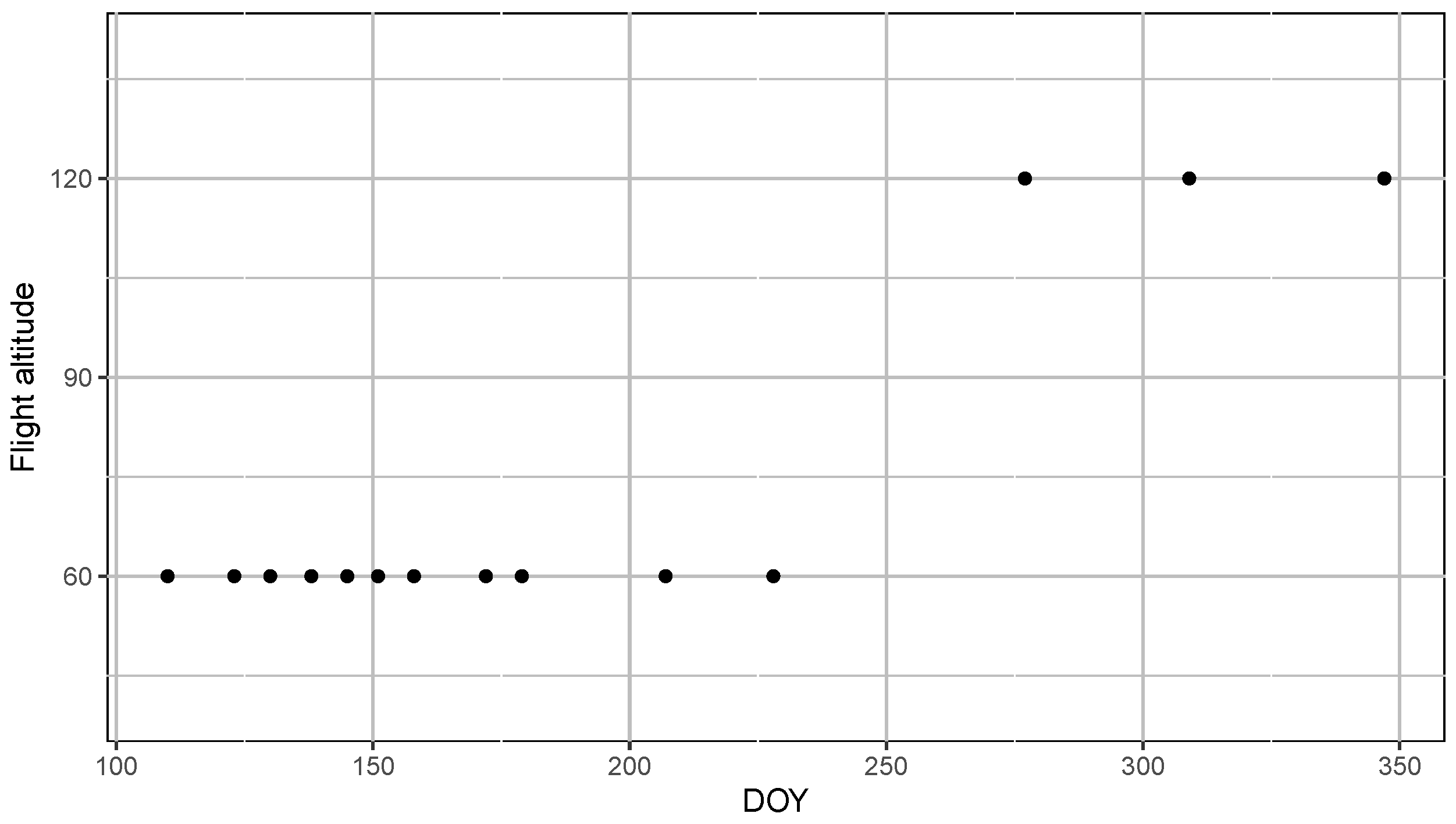
Appendix A.1. Frequency of Data Collection

Figure A1. Overview of the UAV flights (black dots) given in DOY. The y-axis shows the altitude at which the flight was performed.
Remotesensing 15 03599 g0a1

Appendix A.2. Geometric Accuracy (Error) of Each Flight

Table A1. The Euclidian errors (in cm) after 1st order polynomial geometric correction. The lower the error, the more the orthomosaic is geometrically similar to the reference. Correction was performed relative to the reference orthomosaic (26/July). The reference orthomosaic error (italics) is relative to the RTK-measured GCPs.
GCPs20/Apr03/May10/May18/May25/May31/May07/Jun21/Jun28/Jun26/Jul16/Aug04/Oct05/Nov13/Dec
13.22.71.82.52.93.07.12.42.146.32.73.90.66.4
22.22.52.11.71.60.63.02.93.412.62.05.72.83.0
33.32.50.82.30.72.65.92.82.428.53.04.35.63.3
41.40.31.30.92.20.64.72.81.439.11.52.59.80.1
51.72.52.10.61.61.63.30.41.830.21.80.06.56.1
6 61.7
Average2.42.11.61.61.81.74.82.22.236.42.24.15.13.8

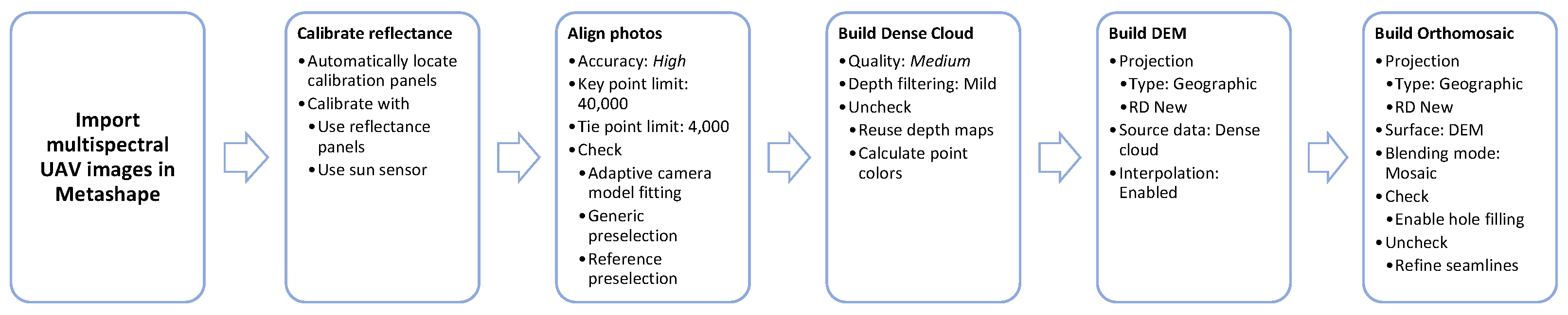
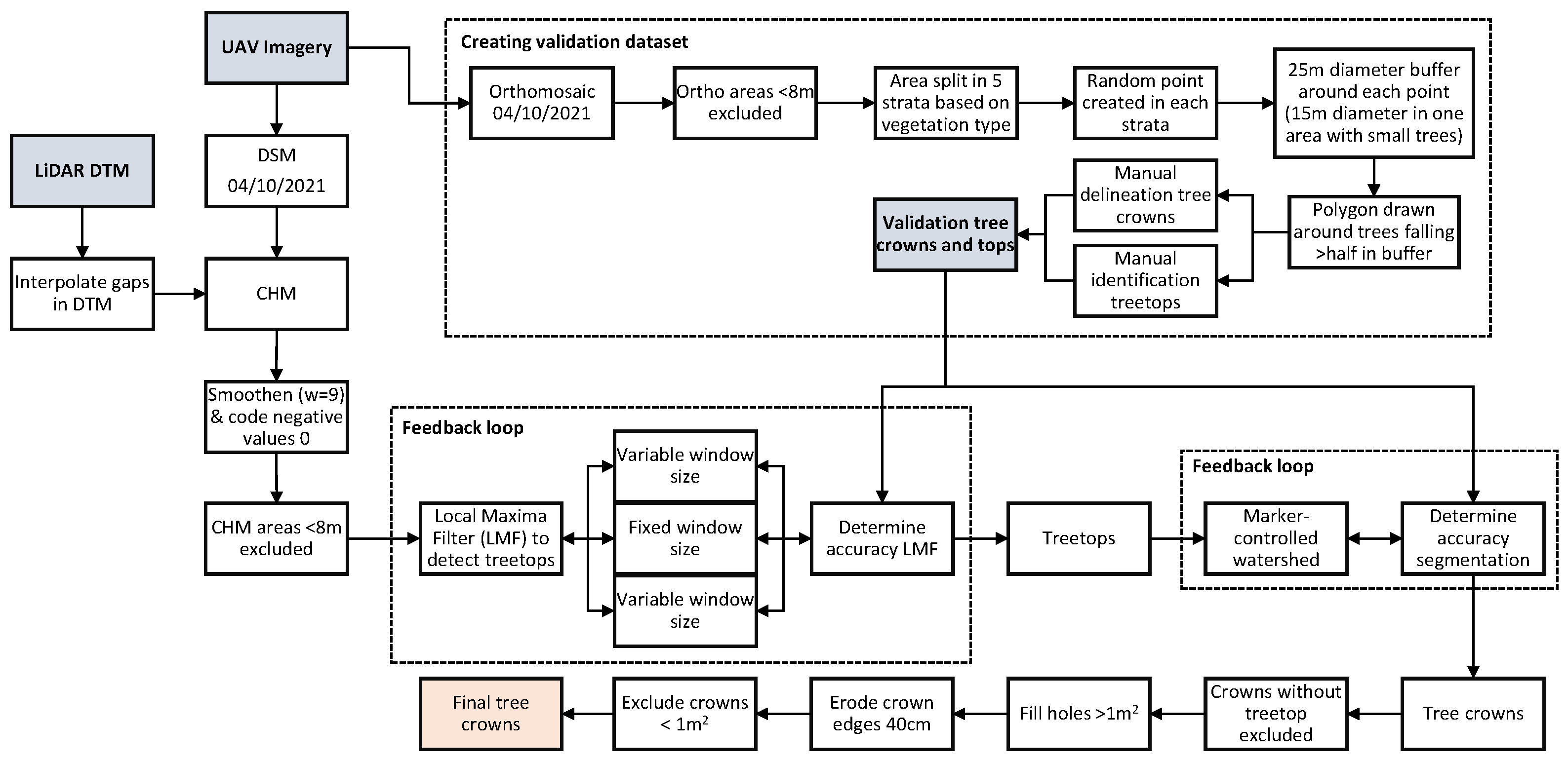
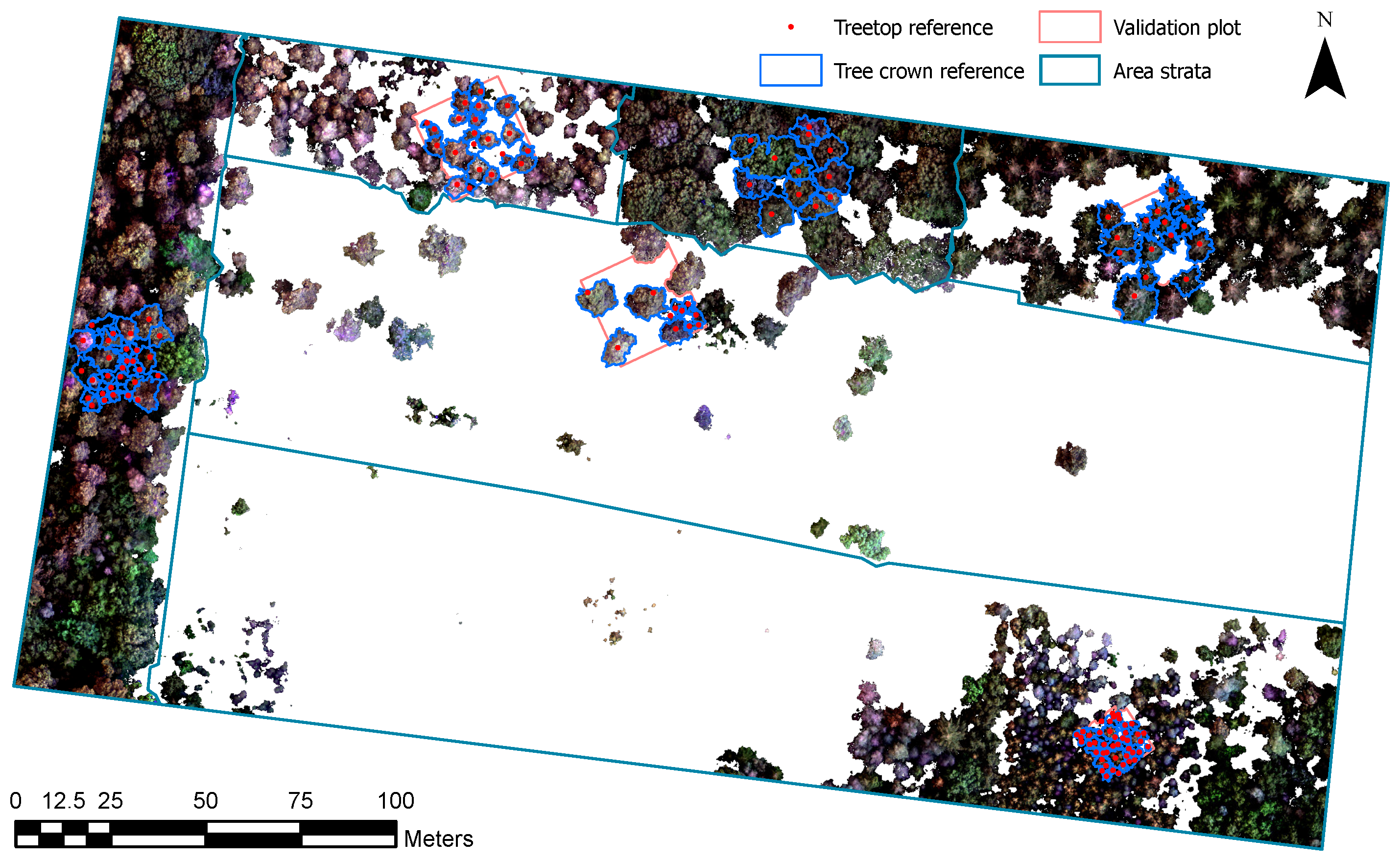
Appendix B. UAV Data Processing

Appendix B.1. Metashape Structure from Motion Steps and Settings

Figure A2. The steps and settings in Agisoft Metashape version 1.5.5 used to transform the raw multispectral UAV images into a DEM and orthomosaic. The bold title of each step is similar to the name of the process within Metashape.
Remotesensing 15 03599 g0a2

Appendix B.2. Workflow of Validation Data Creation and Automatic Crown Segmentation

Figure A3. Schematic representation of the automatic tree crown delineation. The validation process of the segmentation is also schematically included.
Remotesensing 15 03599 g0a3

Appendix B.3. Manually Digitised Validation Data

Figure A4. Reference orthomosaic, with regions lower than 7 m (based on CHM) excluded. All tree tops and crowns falling within a validation plot were manually identified and digitized.
Remotesensing 15 03599 g0a4

Appendix C. Classification

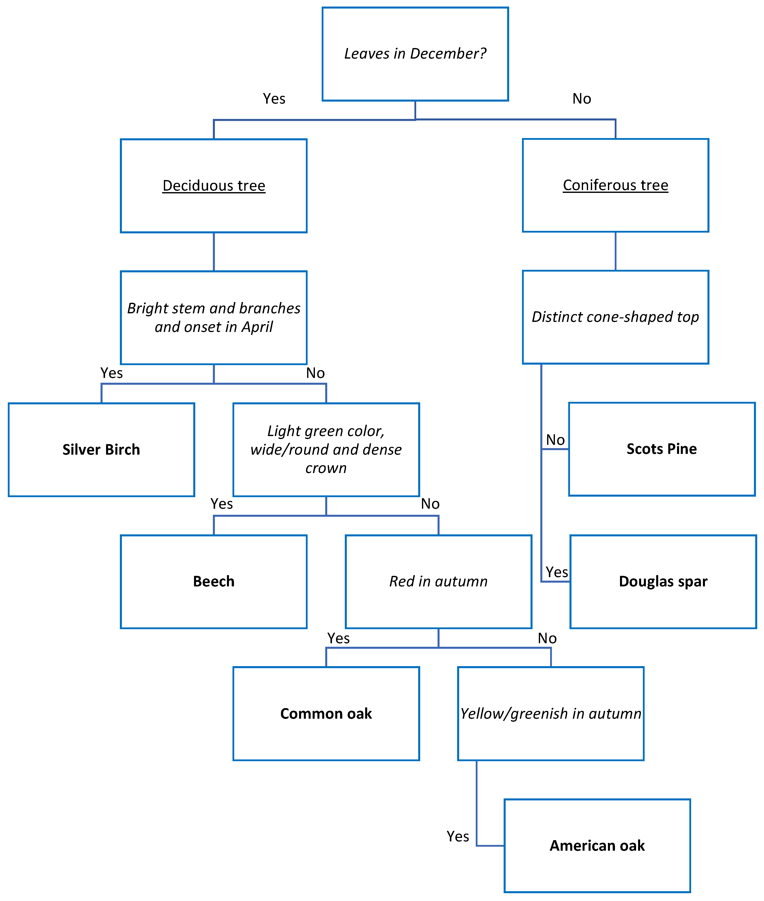
Appendix C.1. Decision Tree for Tree Species Classification

Figure A5. Decision tree for classifying the trees in the study area.
Remotesensing 15 03599 g0a5

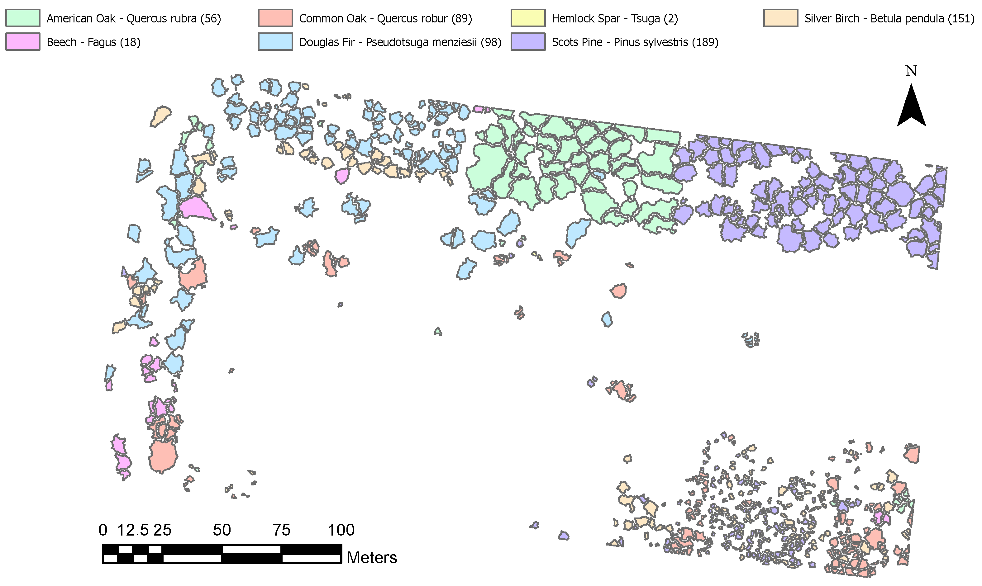
Appendix C.2. Classification Map

Figure A6. Manually classified tree crown segments (n = 603) used for the statistical analysis.
Remotesensing 15 03599 g0a6

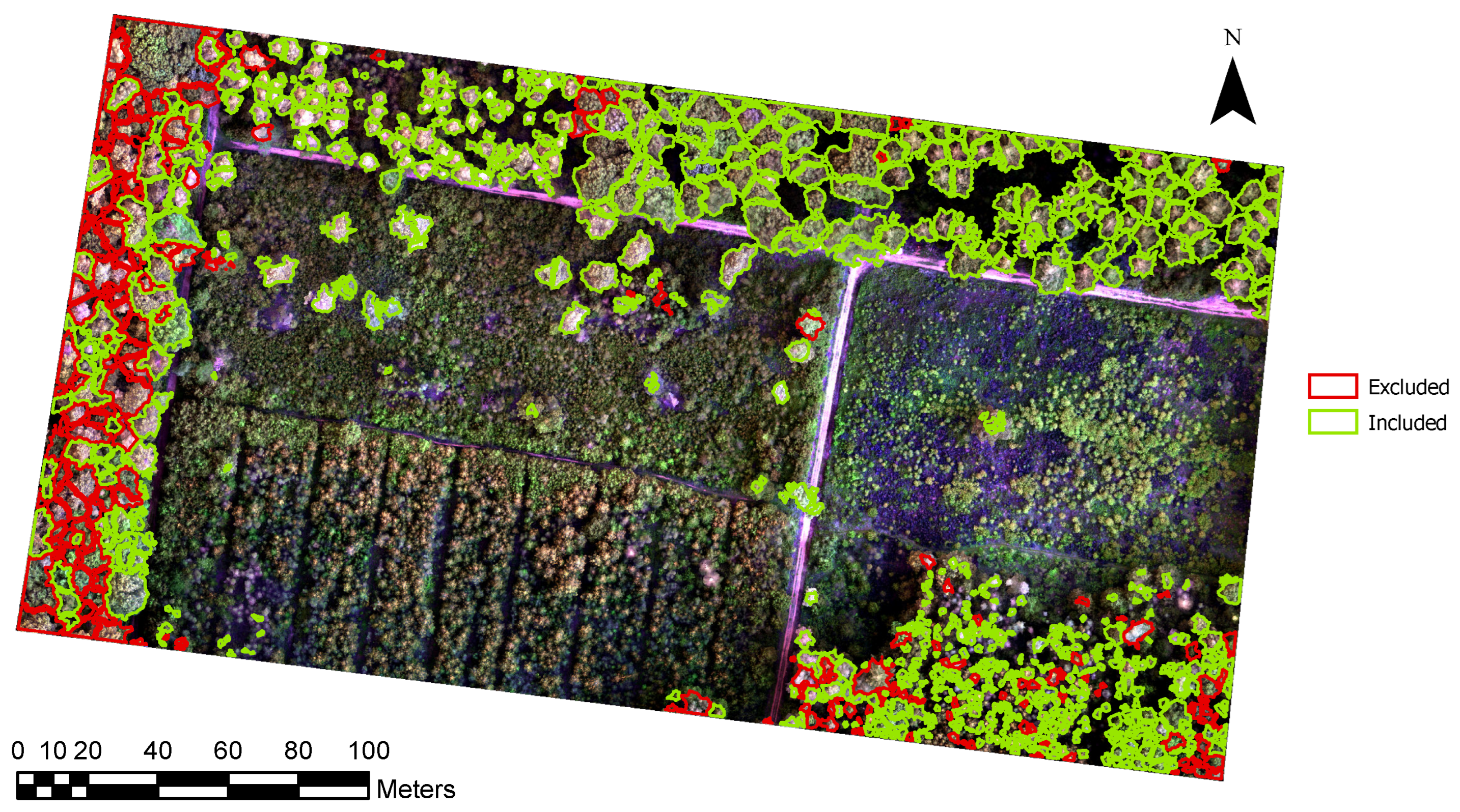
Appendix C.3. Segments Included and Excluded after Manual Classification

Figure A7. Representation of the cleaned segments (n = 876) that were included (n = 603) and excluded (n = 273) after the manual classification. Exclusion was based on segments overlapping multiple species, indefinite classification, or segments that include the ground.
Remotesensing 15 03599 g0a7

Appendix D. Fit Model

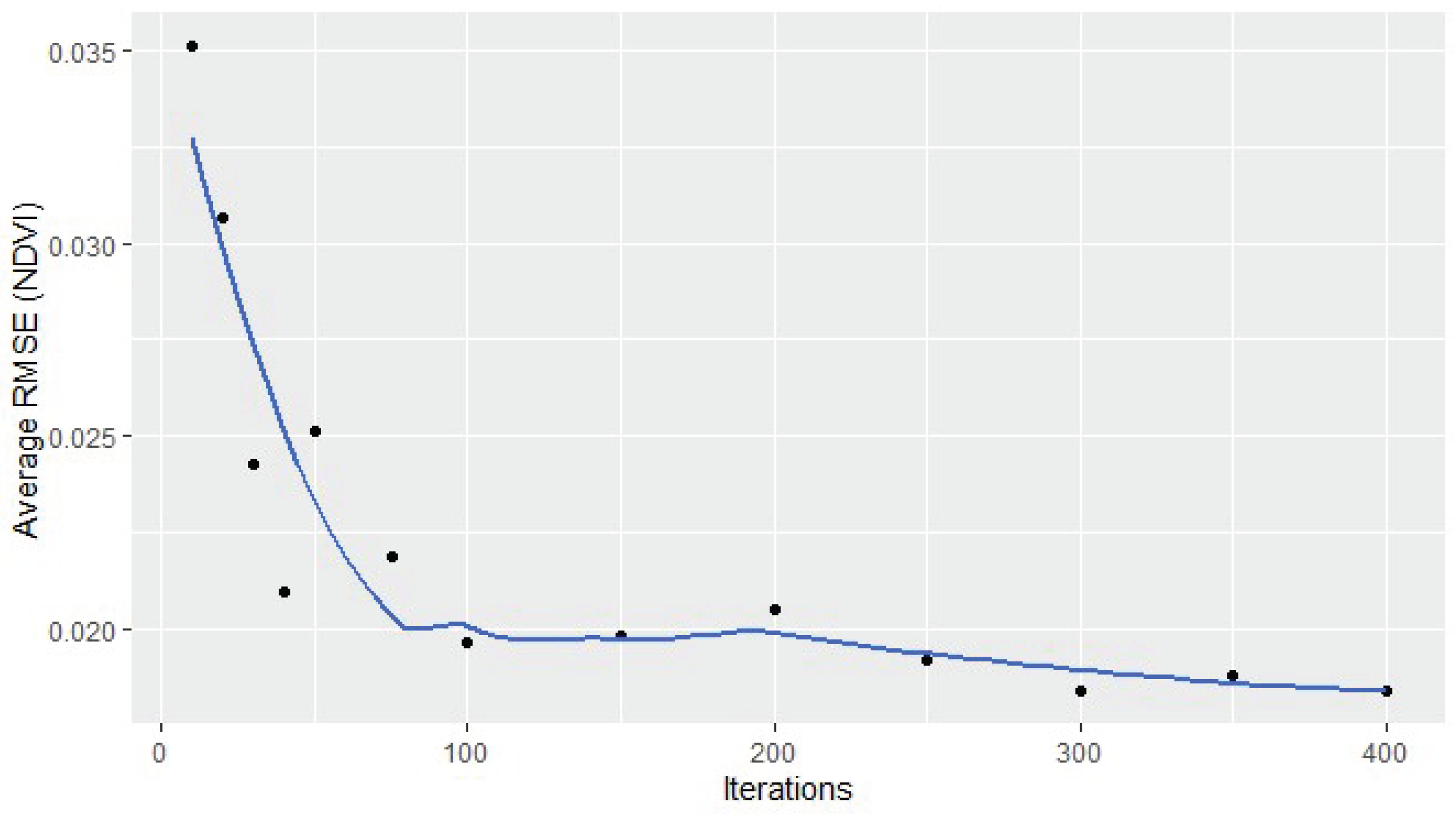
RMSE under Various Iterations

Figure A8. The average RMSE values (black dots) of the double logistic fit for ten randomly selected trees under various iterations. The trend is indicated by a loess curve (blue line) fitted on the average RMSE values.
Remotesensing 15 03599 g0a8

Appendix E. Results

Appendix E.1. Phenology SOS and EOS Estimates

Figure A9. Boxplot showing the SOS and EOS estimates for the deciduous trees, including the outliers. The bold line highlights the median, the box represents the 25th and 75th percentile, the whiskers stretch to 1.5 times the interquartile range from the mean in both directions and the points are identified as outliers. The orange dot indicates the mean.
Remotesensing 15 03599 g0a9

Appendix E.2. EVI2–Derived Spatial Variation SOS and EOS Estimates of the Deciduous Trees

Figure A10. EVI2–derived spatial variation SOS and EOS estimates of the deciduous trees. The SOS and EOS are given in DOY.
Remotesensing 15 03599 g0a10

Appendix E.3. OSAVI–Derived Spatial Variation SOS and EOS Estimates of the Deciduous Trees

Figure A11. OSAVI–derived spatial variation SOS and EOS estimates of the deciduous trees. The SOS and EOS are given in DOY.
Remotesensing 15 03599 g0a11

Appendix E.4. CIre–Derived Spatial Variation SOS and EOS Estimates of the Deciduous Trees

Figure A12. CI r e –derived spatial variation SOS and EOS estimates of the deciduous trees. The SOS and EOS are given in DOY.
Remotesensing 15 03599 g0a12

References

  1. Badeck, F.W.; Bondeau, A.; Böttcher, K.; Doktor, D.; Lucht, W.; Schaber, J.; Sitch, S. Responses of spring phenology to climate change. New Phytol. Found. 2004, 162, 295–309. [Google Scholar] [CrossRef]
  2. Saxe, H.; Cannell, M.G.R.; Johnsen, Ø.R.; Ryan, M.G.; Vourlitis, G. Tree and forest functioning in response to global warming. New Phytol. 2001, 149, 359–388. [Google Scholar] [CrossRef] [PubMed]
  3. Richardson, A.D.; Keenan, T.F.; Migliavacca, M.; Ryu, Y.; Sonnentag, O.; Toomey, M. Climate change, phenology, and phenological control of vegetation feedbacks to the climate system. Agric. For. Meteorol. 2013, 169, 156–173. [Google Scholar] [CrossRef]
  4. Peñuelas, J.; Rutishauser, T.; Filella, I. A conceptual framework explains how individual species’ responses to climate warming affect the length of the growing season. Phenol. Feed. Clim. Chang. 2009, 324, 5929. [Google Scholar] [CrossRef]
  5. Estrella, N.; Menzel, A. Responses of leaf colouring in four deciduous tree species to climate and weather in Germany. Clim. Res. 2006, 32, 253–267. [Google Scholar] [CrossRef] [Green Version]
  6. Rosenzweig, C.; Casassa, G.; Karoly, D.J.; Imeson, A.; Liu, C.; Menzel, A.; Rawlins, S.; Root, T.L.; Seguin, B.; Tryjanowski, P. Assessment of observed changes and responses in natural and managed systems. In Climate Change 2007: Impacts, Adaptation and Vulnerability. Contribution of Working Group II to the Fourth Assessment Report of the Intergovernmental Panel on Climate Change; Parry, M.L., Ed.; Cambridge Univerisity Press: Cambridge, UK, 2007; pp. 79–113. [Google Scholar]
  7. Richardson, A.D.; Baily, A.S.; Denny, E.G.; Martin, C.W.; O’Keefe, J. Phenology of a northern hardwood forest canopy. Glob. Chang. Biol. 2006, 12, 1174–1188. [Google Scholar] [CrossRef] [Green Version]
  8. Melaas, E.K.; Friedl, M.A.; Zhu, Z. Detecting interannual variation in deciduous broadleaf forest phenology using Landsat TM/ETM+ data. Remote Sens. Environ. 2013, 132, 176–185. [Google Scholar] [CrossRef]
  9. Pastor-Guzman, J.; Dash, J.; Atkinson, P.M. Remote sensing of mangrove forest phenology and its environmental drivers. Remote Sens. Environ. 2018, 205, 71–84. [Google Scholar] [CrossRef] [Green Version]
  10. Pennec, A.; Gond, V.; Sabatier, D. Tropical forest phenology in French Guiana from MODIS time series. Remote Sens. Lett. 2011, 2, 337–345. [Google Scholar] [CrossRef]
  11. Walker, J.; de Beurs, K.; Wynne, R.; Gao, F. Evaluation of Landsat and MODIS data fusion products for analysis of dryland forest phenology. Remote Sens. Environ. 2012, 117, 381–393. [Google Scholar] [CrossRef]
  12. Han, Q. Remote sensing-based quantification of spatial variation in canopy phenology of four dominant tree species in Europe. J. Appl. Remote Sens. 2013, 7, 073485. [Google Scholar] [CrossRef] [Green Version]
  13. Delbart, N.; Kergoat, L.; Le Toan, T.; Lhermitte, J.; Picard, G. Determination of phenological dates in boreal regions using normalized difference water index. Remote Sens. Environ. 2005, 97, 26–38. [Google Scholar] [CrossRef] [Green Version]
  14. Jones, M.O.; Jones, L.A.; Kimball, J.S.; McDonald, K.C. Satellite passive microwave remote sensing for monitoring global land surface phenology. Remote Sens. Environ. 2011, 115, 1081–1089. [Google Scholar] [CrossRef]
  15. Zhang, X.; Friedl, M.A.; Schaaf, C.B.; Strahler, A.H.; Hodges, J.C.; Gao, F.; Reed, B.C.; Huete, A. Monitoring vegetation phenology using MODIS. Remote Sens. Environ. 2003, 84, 471–475. [Google Scholar] [CrossRef]
  16. Pinzon, J.; Tucker, C. A Non-Stationary 1981–2012 AVHRR NDVI3g Time Series. Remote Sens. 2014, 6, 6929. [Google Scholar] [CrossRef] [Green Version]
  17. Tucker, C.J.; Pinzon, J.E.; Brown, M.E.; Slayback, D.A.; Pak, E.W.; Mahoney, R.; Vermote, E.F.; El Saleous, N. An extended AVHRR 8-km NDVI dataset compatible with MODIS and SPOT vegetation NDVI data. Int. J. Remote Sens. 2005, 26, 4485–4498. [Google Scholar] [CrossRef]
  18. White, M.A.; de Beurs, K.M.; Didan, K.; Inouye, D.W.; Richarson, A.D.; Jensen, O.P.; O’Keefe, J.; Zhang, G.; Nemani, R.R.; van Leeuweb, W.J.D.; et al. Intercomparison, interpretation, and assessment of spring phenology in North America estimated from remote sensing for 1982–2006. Glob. Chang. Biol. 2009, 15, 2335–2359. [Google Scholar] [CrossRef]
  19. Polgar, C.A.; Primack, R.B. Leaf-out phenology of temperate woody plants: From trees to ecosystems. New Phytol. 2011, 191, 926–941. [Google Scholar] [CrossRef]
  20. Liu, Y.; Hill, M.J.; Zhang, X.; Wang, Z.; Richardson, A.D.; Hufkens, K.; Filippa, G.; Baldocchi, D.D.; Ma, S.; Verfaillie, J.; et al. Using data from Landsat, MODIS, VIIRS and PhenoCams to monitor the phenology of California oak/grass savanna and open grassland across spatial scales. Agric. For. Meteorol. 2017, 237–238, 311–325. [Google Scholar] [CrossRef]
  21. Berra, E.F.; Gaulton, R.; Barr, S. Assessing spring phenology of a temperate woodland: A multiscale comparison of ground, unmanned aerial vehicle and Landsat satellite observations. Remote Sens. Environ. 2019, 223, 229–242. [Google Scholar] [CrossRef]
  22. Sparks, T.H.; Menzel, A. Observed changes in seasons: An overview. Int. J. Climatol. 2002, 22, 1715–1725. [Google Scholar] [CrossRef]
  23. Fitter, A.H.; Fitter, R.S.R. Rapid Changes in Flowering Time in British Plants. Science 2002, 296, 1689–1691. [Google Scholar] [CrossRef] [PubMed]
  24. Denéchère, R.; Delpierre, N.; Apostol, E.N.; Berveiller, D.; Bonne, F.; Cole, E.; Delzon, S.; Dufrêne, E.; Gressler, E.; Jean, F.; et al. The within-population variability of leaf spring and autumn phenology is influenced by temperature in temperate deciduous trees. Int. J. Biometeorol. 2021, 65, 369–379. [Google Scholar] [CrossRef]
  25. Delpierre, N.; Guillemot, J.; Dufrêne, E.; Cecchini, S.; Nicolas, M. Tree phenological ranks repeat from year to year and correlate with growth in temperate deciduous forests. Agric. For. Meteorol. 2017, 234–235, 1–10. [Google Scholar] [CrossRef]
  26. D’Odorico, P.; Besik, A.; Wong, C.Y.; Isabel, N.; Ensminger, I. High-throughput drone-based remote sensing reliably tracks phenology in thousands of conifer seedlings. New Phytol. 2020, 226, 1667–1681. [Google Scholar] [CrossRef]
  27. Borra-Serrano, I.; Swaef, T.D.; Quataert, P.; Aper, J.; Saleem, A.; Saeys, W.; Somers, B.; Roldán-Ruiz, I.; Lootens, P. Closing the phenotyping gap: High resolution UAV time series for soybean growth analysis provides objective data from field trials. Remote Sens. 2020, 12, 1644. [Google Scholar] [CrossRef]
  28. Ampatzidis, Y.; Partel, V. UAV-based high throughput phenotyping in citrus utilizing multispectral imaging and artificial intelligence. Remote Sens. 2019, 11, 410. [Google Scholar] [CrossRef] [Green Version]
  29. Mahlein, A.K. Plant Disease Detection by Imaging Sensors – Parallels and Specific Demands for Precision Agriculture and Plant Phenotyping. Plant Dis. 2016, 100, 241–251. [Google Scholar] [CrossRef] [Green Version]
  30. Shakoor, N.; Lee, S.; Mockler, T.C. High throughput phenotyping to accelerate crop breeding and monitoring of diseases in the field. Curr. Opin. Plant Biol. 2017, 38, 184–192. [Google Scholar] [CrossRef]
  31. Fawcett, D.; Bennie, J.; Anderson, K. Monitoring spring phenology of individual tree crowns using drone-acquired NDVI data. Remote Sens. Ecol. Conserv. 2021, 7, 227–244. [Google Scholar] [CrossRef]
  32. Budianti, N.; Mizunaga, H.; Iio, A. Crown structure explains the discrepancy in leaf phenology metrics derived from ground-and uav-based observations in a japanese cool temperate deciduous forest. Forests 2021, 12, 425. [Google Scholar] [CrossRef]
  33. Dingle Robertson, L.; King, D.J. Comparison of pixel- and object-based classification in land cover change mapping. Int. J. Remote Sens. 2011, 32, 1505–1529. [Google Scholar] [CrossRef]
  34. Cai, S.; Liu, D. A comparison of object-based and contextual pixel-based classifications using high and medium spatial resolution images. Remote Sens. Lett. 2013, 4, 998–1007. [Google Scholar] [CrossRef]
  35. Pande-Chhetri, R.; Abd-Elrahman, A.; Liu, T.; Morton, J.; Wilhelm, V.L. Object-based classification of wetland vegetation using very high-resolution unmanned air system imagery. Eur. J. Remote Sens. 2017, 50, 564–576. [Google Scholar] [CrossRef] [Green Version]
  36. Hamylton, S.; Morris, R.; Carvalho, R.; Roder, N.; Barlow, P.; Mills, K.; Wang, L. Evaluating techniques for mapping island vegetation from unmanned aerial vehicle (UAV) images: Pixel classification, visual interpretation and machine learning approaches. Int. J. Appl. Earth Obs. Geoinf. 2020, 89, 102085. [Google Scholar] [CrossRef]
  37. Hossain, M.D.; Chen, D. Segmentation for Object-Based Image Analysis (OBIA): A review of algorithms and challenges from remote sensing perspective. ISPRS J. Photogramm. Remote Sens. 2019, 150, 115–134. [Google Scholar] [CrossRef]
  38. Ke, Y.; Quackenbush, L.J. A review of methods for automatic individual tree-crown detection and delineation from passive remote sensing. Int. J. Remote Sens. 2011, 32, 4725–4747. [Google Scholar] [CrossRef]
  39. Wagner, F.H.; Ferreira, M.P.; Sanchez, A.; Hirye, M.C.; Zortea, M.; Gloor, E.; Phillips, O.L.; de Souza Filho, C.R.; Shimabukuro, Y.E.; Aragão, L.E. Individual tree crown delineation in a highly diverse tropical forest using very high resolution satellite images. ISPRS J. Photogramm. Remote Sens. 2018, 145, 362–377. [Google Scholar] [CrossRef]
  40. Gu, J.; Grybas, H.; Congalton, R.G. A comparison of forest tree crown delineation from unmanned aerial imagery using canopy height models vs. spectral lightness. Forests 2020, 11, 605. [Google Scholar] [CrossRef]
  41. Li, D.; Zhang, G.; Wu, Z.; Yi, L. An Edge Embedded Marker-Based Watershed Algorithm for High Spatial Resolution Remote Sensing Image Segmentation. IEEE Trans. Image Process. 2010, 19, 2781–2787. [Google Scholar] [CrossRef]
  42. Cai, Y.; Tong, X.; Shu, R. Multi-scale segmentation of remote sensing image based on watershed transformation. In Proceedings of the 2009 Joint Urban Remote Sensing Event, Shanghai, China, 20–22 May 2009; pp. 1–6. [Google Scholar] [CrossRef]
  43. Wang, M.; Li, R. Segmentation of High Spatial Resolution Remote Sensing Imagery Based on Hard-Boundary Constraint and Two-Stage Merging. IEEE Trans. Geosci. Remote Sens. 2014, 52, 5712–5725. [Google Scholar] [CrossRef]
  44. Mylonas, S.; Stavrakoudis, D.; Theocharis, J.; Mastorocostas, P. A Region-Based GeneSIS Segmentation Algorithm for the Classification of Remotely Sensed Images. Remote Sens. 2015, 7, 2474–2508. [Google Scholar] [CrossRef] [Green Version]
  45. Gaetano, R.; Masi, G.; Poggi, G.; Verdoliva, L.; Scarpa, G. Marker-controlled watershed-based segmentation of multiresolution remote sensing images. IEEE Trans. Geosci. Remote Sens. 2015, 53, 2987–3004. [Google Scholar] [CrossRef]
  46. Klosterman, S.; Melaas, E.; Wang, J.; Martinez, A.; Frederick, S.; O’Keefe, J.; Orwig, D.A.; Wang, Z.; Sun, Q.; Schaaf, C.; et al. Fine-scale perspectives on landscape phenology from unmanned aerial vehicle (UAV) photography. Agric. For. Meteorol. 2018, 248, 397–407. [Google Scholar] [CrossRef]
  47. Park, J.Y.; Muller-Landau, H.C.; Lichstein, J.W.; Rifai, S.W.; Dandois, J.P.; Bohlman, S.A. Quantifying leaf phenology of individual trees and species in a tropical forest using unmanned aerial vehicle (UAV) images. Remote Sens. 2019, 11, 1534. [Google Scholar] [CrossRef] [Green Version]
  48. Tucker, C.J. Red and photographic infrared linear combinations for monitoring vegetation. Remote Sens. Environ. 1979, 8, 127–150. [Google Scholar] [CrossRef] [Green Version]
  49. Marcial-Pablo, M.d.J.; Gonzalez-Sanchez, A.; Jimenez-Jimenez, S.I.; Ontiveros-Capurata, R.E.; Ojeda-Bustamante, W. Estimation of vegetation fraction using RGB and multispectral images from UAV. Int. J. Remote Sens. 2019, 40, 420–438. [Google Scholar] [CrossRef]
  50. Yin, G.; Verger, A.; Filella, I.; Descals, A.; Peñuelas, J. Divergent Estimates of Forest Photosynthetic Phenology Using Structural and Physiological Vegetation Indices. Geophys. Res. Lett. 2020, 47, e2020GL089167. [Google Scholar] [CrossRef]
  51. Wong, C.Y.S.; D’Odorico, P.; Bhathena, Y.; Arain, M.A.; Ensminger, I. Carotenoid based vegetation indices for accurate monitoring of the phenology of photosynthesis at the leaf-scale in deciduous and evergreen trees. Remote Sens. Environ. 2019, 233, 111407. [Google Scholar] [CrossRef]
  52. Thapa, S.; Garcia Millan, V.E.; Eklundh, L. Assessing forest phenology: A multi-scale comparison of near-surface (UAV, spectral reflectance sensor, phenocam) and satellite (MODIS, sentinel-2) remote sensing. Remote Sens. 2021, 13, 1597. [Google Scholar] [CrossRef]
  53. Huang, S.; Tang, L.; Hupy, J.P.; Wang, Y.; Shao, G. A commentary review on the use of normalized difference vegetation index (NDVI) in the era of popular remote sensing. J. For. Res. 2021, 32, 1–6. [Google Scholar] [CrossRef]
  54. Gitelson, A.A.; Gritz, Y.; Merzlyak, M.N. Relationships between leaf chlorophyll content and spectral reflectance and algorithms for non-destructive chlorophyll assessment in higher plant leaves. J. Plant Physiol. 2003, 160, 271–282. [Google Scholar] [CrossRef] [PubMed]
  55. KNMI. Weerstations: Dagwaarnemingen. Temperature and Precipitation Were Derived from Historic Daily Temperature (TG) and Rainfall (RH) Measurements Conducted by the KNMI at Location of Deelen Which Is 15 km from the Study Area. Historic Temperature Measurements Date Back to 1960 and Rainfall to 1983. 2022. Available online: https://www.daggegevens.knmi.nl/klimatologie/daggegevens (accessed on 2 April 2022).
  56. Tu, Y.H.; Phinn, S.; Johansen, K.; Robson, A. Assessing radiometric correction approaches for multi-spectral UAS imagery for horticultural applications. Remote Sens. 2018, 10, 1684. [Google Scholar] [CrossRef] [Green Version]
  57. Assmann, J.J.; Kerby, J.T.; Cunliffe, A.M.; Myers-Smith, I.H. Vegetation monitoring using multispectral sensors—Best practices and lessons learned from high latitudes. J. Unmanned Veh. Syst. 2019, 7, 54–75. [Google Scholar] [CrossRef] [Green Version]
  58. Agisoft LLC. Metashape, 2019. Available online: https://www.agisoft.com/downloads/installer/ (accessed on 9 March 2022).
  59. ESRI. ArcGIS Pro, 2021. Available online: https://www.esri.com/en-us/arcgis/products/arcgis-pro/overview (accessed on 9 March 2022).
  60. Berra, E.F.; Gaulton, R.; Barr, S. Commercial Off-the-Shelf Digital Cameras on Unmanned Aerial Vehicles for Multitemporal Monitoring of Vegetation Reflectance and NDVI. IEEE Trans. Geosci. Remote Sens. 2017, 55, 4878–4886. [Google Scholar] [CrossRef] [Green Version]
  61. Panagiotidis, D.; Abdollahnejad, A.; Surový, P.; Chiteculo, V. Determining tree height and crown diameter from high-resolution UAV imagery. Int. J. Remote Sens. 2017, 38, 2392–2410. [Google Scholar] [CrossRef]
  62. AHN. AHN 3 DTM, 2019. Available online: https://app.pdok.nl/ahn3-downloadpage/ (accessed on 10 March 2022).
  63. Mohan, M.; Leite, R.V.; Broadbent, E.N.; Wan Mohd Jaafar, W.S.; Srinivasan, S.; Bajaj, S.; Dalla Corte, A.P.; do Amaral, C.H.; Gopan, G.; Saad, S.N.M.; et al. Individual tree detection using UAV-lidar and UAV-SfM data: A tutorial for beginners. Open Geosci. 2021, 13, 1028–1039. [Google Scholar] [CrossRef]
  64. Roussel, J.R.; Auty, D. lidR, 2021. Available online: https://cran.r-project.org/web/packages/lidR/index.html (accessed on 11 March 2022).
  65. Doruska, P.F.; Burkhart, H.E. Modeling the diameter and locational distribution of branches within the crowns of loblolly pine trees in unthinned plantations. Can. J. For. Res. 1994, 24, 2362–2376. [Google Scholar] [CrossRef]
  66. Popescu, S.C.; Wynne, R.H. Seeing the Trees in the Forest. Photogramm. Eng. Remote Sens. 2004, 70, 589–604. [Google Scholar] [CrossRef] [Green Version]
  67. Plowright, A.; Roussel, J.R. ForestTools, 2021. Available online: https://cran.r-project.org/web/packages/ForestTools/index.html (accessed on 13 March 2022).
  68. Meyer, F.; Beucher, S. Morphological segmentation. J. Vis. Commun. Image Represent. 1990, 1, 21–46. [Google Scholar] [CrossRef]
  69. Strimas-Mackey, M. Smoothr, 2021. Available online: https://cran.r-project.org/web/packages/smoother/index.html (accessed on 14 March 2022).
  70. Zeng, L.; Wardlow, B.D.; Xiang, D.; Hu, S.; Li, D. A review of vegetation phenological metrics extraction using time-series, multispectral satellite data. Remote Sens. Environ. 2020, 237, 111511. [Google Scholar] [CrossRef]
  71. Beck, P.S.; Atzberger, C.; Høgda, K.A.; Johansen, B.; Skidmore, A.K. Improved monitoring of vegetation dynamics at very high latitudes: A new method using MODIS NDVI. Remote Sens. Environ. 2006, 100, 321–334. [Google Scholar] [CrossRef]
  72. Forkel, W.M. Greenbrown, 2015. Available online: http://greenbrown.r-forge.r-project.org/ (accessed on 16 March 2022).
  73. Cao, R.; Chen, J.; Shen, M.; Tang, Y. An improved logistic method for detecting spring vegetation phenology in grasslands from MODIS EVI time-series data. Agric. For. Meteorol. 2015, 200, 9–20. [Google Scholar] [CrossRef]
  74. Clinton, N.; Holt, A.; Scarborough, J.; Yan, L.; Gong, P. Accuracy Assessment Measures for Object-based Image Segmentation Goodness. Photogramm. Eng. Remote Sens. 2010, 76, 289–299. [Google Scholar] [CrossRef]
  75. Winter, S. Location similarity of regions. ISPRS J. Photogramm. Remote Sens. 2000, 55, 189–200. [Google Scholar] [CrossRef]
  76. Sellers, P.J. Canopy reflectance, photosynthesis and transpiration. Int. J. Remote Sens. 1985, 6, 1335–1372. [Google Scholar] [CrossRef] [Green Version]
  77. Vitasse, Y.; Lenz, A.; Körner, C. The interaction between freezing tolerance and phenology in temperate deciduous trees. Front. Plant Sci. 2014, 5, 541. [Google Scholar] [CrossRef] [Green Version]
  78. Dong, T.; Meng, J.; Shang, J.; Liu, J.; Wu, B. Evaluation of Chlorophyll-Related Vegetation Indices Using Simulated Sentinel-2 Data for Estimation of Crop Fraction of Absorbed Photosynthetically Active Radiation. IEEE J. Sel. Top. Appl. Earth Obs. Remote Sens. 2015, 8, 4049–4059. [Google Scholar] [CrossRef]
  79. Nguy-Robertson, A.L.; Peng, Y.; Gitelson, A.A.; Arkebauer, T.J.; Pimstein, A.; Herrmann, I.; Karnieli, A.; Rundquist, D.C.; Bonfil, D.J. Estimating green LAI in four crops: Potential of determining optimal spectral bands for a universal algorithm. Agric. For. Meteorol. 2014, 192-193, 140–148. [Google Scholar] [CrossRef]
  80. Schlemmer, M.; Gitelson, A.; Schepers, J.; Ferguson, R.; Peng, Y.; Shanahan, J.; Rundquist, D. Remote estimation of nitrogen and chlorophyll contents in maize at leaf and canopy levels. Int. J. Appl. Earth Obs. Geoinf. 2013, 25, 47–54. [Google Scholar] [CrossRef] [Green Version]
  81. Adams, W.; Zarter, R.; Ebbert, V.; Demmig-Adams, B. Photoprotective Strategies of Overwintering Evergreens. BioScience 2004, 54, 41–49. [Google Scholar] [CrossRef]
  82. Fu, Y.H.; Piao, S.; Op de Beeck, M.; Cong, N.; Zhao, H.; Zhang, Y.; Menzel, A.; Janssens, I.A. Recent spring phenology shifts in western Central Europe based on multiscale observations. Glob. Ecol. Biogeogr. 2014, 23, 1255–1263. [Google Scholar] [CrossRef]
  83. Jeong, S.J.; Schimel, D.; Frankenberg, C.; Drewry, D.T.; Fisher, J.B.; Verma, M.; Berry, J.A.; Lee, J.E.; Joiner, J. Application of satellite solar-induced chlorophyll fluorescence to understanding large-scale variations in vegetation phenology and function over northern high latitude forests. Remote Sens. Environ. 2017, 190, 178–187. [Google Scholar] [CrossRef]
  84. Badgley, G.; Field, C.B.; Berry, J.A. Canopy near-infrared reflectance and terrestrial photosynthesis. Sci. Adv. 2017, 3, 1602244. [Google Scholar] [CrossRef] [Green Version]
  85. Tanaka, S.; Kawamura, K.; Maki, M.; Muramoto, Y.; Yoshida, K.; Akiyama, T. Spectral Index for Quantifying Leaf Area Index of Winter Wheat by Field Hyperspectral Measurements: A Case Study in Gifu Prefecture, Central Japan. Remote Sens. 2015, 7, 5329–5346. [Google Scholar] [CrossRef] [Green Version]
  86. Hashimoto, N.; Saito, Y.; Maki, M.; Homma, K. Simulation of reflectance and vegetation indices for unmanned aerial vehicle (UAV) monitoring of paddy fields. Remote Sens. 2019, 11, 2119. [Google Scholar] [CrossRef] [Green Version]
  87. Kikuzawa, K. Phenological and morphological adaptations to the light environment in two woody and two herbaceous plant species. Funct. Ecol. 2003, 17, 29–38. [Google Scholar] [CrossRef]
  88. Mariën, B.; Balzarolo, M.; Dox, I.; Leys, S.; Lorène, M.J.; Geron, C.; Portillo-Estrada, M.; AbdElgawad, H.; Asard, H.; Campioli, M. Detecting the onset of autumn leaf senescence in deciduous forest trees of the temperate zone. New Phytol. 2019, 224, 166–176. [Google Scholar] [CrossRef] [PubMed]
  89. Medvigy, D.; Jeong, S.J.; Clark, K.L.; Skowronski, N.S.; Schäfer, K.V.R. Effects of seasonal variation of photosynthetic capacity on the carbon fluxes of a temperate deciduous forest. J. Geophys. Res. Biogeosci. 2013, 118, 1703–1714. [Google Scholar] [CrossRef]
  90. de Natuurkalender. Natuurkalender. 2021. Available online: https://www.naturetoday.com/intl/nl/observations/natuurkalender/sightings/view-sightings (accessed on 30 March 2022).
  91. Wu, S.; Wang, J.; Yan, Z.; Song, G.; Chen, Y.; Ma, Q.; Deng, M.; Wu, Y.; Zhao, Y.; Guo, Z.; et al. Monitoring tree-crown scale autumn leaf phenology in a temperate forest with an integration of PlanetScope and drone remote sensing observations. ISPRS J. Photogramm. Remote Sens. 2021, 171, 36–48. [Google Scholar] [CrossRef]
  92. Kuster, T.M.; Dobbertin, M.; Günthardt-Goerg, M.S.; Schaub, M.; Arend, M. A Phenological Timetable of Oak Growth under Experimental Drought and Air Warming. PLoS ONE 2014, 9, e89724. [Google Scholar] [CrossRef] [PubMed]
  93. Leslie, A.; Mencuccini, M.; Perks, M. A resource capture efficiency index to compare differences in early growth of four tree species in northern England. iForest-Biogeosci. For. 2017, 10, 397–405. [Google Scholar] [CrossRef]
  94. Vander Mijnsbrugge, K.; Janssens, A. Differentiation and Non-Linear Responses in Temporal Phenotypic Plasticity of Seasonal Phenophases in a Common Garden of Crataegus monogyna Jacq. Forests 2019, 10, 293. [Google Scholar] [CrossRef] [Green Version]
  95. Lim, Y.S.; La, P.H.; Park, J.S.; Lee, M.H.; Pyeon, M.W.; Kim, J.I. Calculation of Tree Height and Canopy Crown from Drone Images Using Segmentation. J. Korean Soc. Surv. Geod. Photogramm. Cartogr. 2015, 33, 605–614. [Google Scholar] [CrossRef] [Green Version]
  96. Xu, Z.; Shen, X.; Cao, L.; Coops, N.C.; Goodbody, T.R.; Zhong, T.; Zhao, W.; Sun, Q.; Ba, S.; Zhang, Z.; et al. Tree species classification using UAS-based digital aerial photogrammetry point clouds and multispectral imageries in subtropical natural forests. Int. J. Appl. Earth Obs. Geoinf. 2020, 92, 102173. [Google Scholar] [CrossRef]
  97. Belcore, E.; Wawrzaszek, A.; Wozniak, E.; Grasso, N.; Piras, M. Individual tree detection from UAV imagery using Hölder exponent. Remote Sens. 2020, 12, 2407. [Google Scholar] [CrossRef]
  98. Fawcett, D.; Azlan, B.; Hill, T.C.; Kho, L.K.; Bennie, J.; Anderson, K. Unmanned aerial vehicle (UAV) derived structure-from-motion photogrammetry point clouds for oil palm ( <i>Elaeis guineensis</i> ) canopy segmentation and height estimation. Int. J. Remote Sens. 2019, 40, 7538–7560. [Google Scholar] [CrossRef] [Green Version]
  99. Duncanson, L.; Cook, B.; Hurtt, G.; Dubayah, R. An efficient, multi-layered crown delineation algorithm for mapping individual tree structure across multiple ecosystems. Remote Sens. Environ. 2014, 154, 378–386. [Google Scholar] [CrossRef]
  100. van Iersel, W.; Straatsma, M.; Addink, E.; Middelkoop, H. Monitoring height and greenness of non-woody floodplain vegetation with UAV time series. ISPRS J. Photogramm. Remote Sens. 2018, 141, 112–123. [Google Scholar] [CrossRef]
  101. Atkins, J.W.; Stovall, A.E.; Yang, X. Mapping temperate forest phenology using tower, UAV, and ground-based sensors. Drones 2020, 4, 1–15. [Google Scholar] [CrossRef]
  102. Schiefer, F.; Kattenborn, T.; Frick, A.; Frey, J.; Schall, P.; Koch, B.; Schmidtlein, S. Mapping forest tree species in high resolution UAV-based RGB-imagery by means of convolutional neural networks. ISPRS J. Photogramm. Remote Sens. 2020, 170, 205–215. [Google Scholar] [CrossRef]
  103. Zhang, C.; Atkinson, P.M.; George, C.; Wen, Z.; Diazgranados, M.; Gerard, F. Identifying and mapping individual plants in a highly diverse high-elevation ecosystem using UAV imagery and deep learning. ISPRS J. Photogramm. Remote Sens. 2020, 169, 280–291. [Google Scholar] [CrossRef]
Figure 1. Composite orthomosaic of 4 October 2021 from the MicaSense camera of the study area near Wageningen. The area is divided into six areas (blue lines): dense mixed (west), coniferous mixed (northwest), deciduous (mid-north), coniferous (northeast), sparse mixed (center), and small (south). The white crosses show the locations of the RTK-measured GCPs. The red crosses indicate the natural static objects used as GCPs (1: tree stump, 2: bench, 3: stem on ground, 4: small pointy tree, 5: woodblock, 6: circular ground vegetation, and 7: stem on ground). The green star indicates the landing and take-off location.
Remotesensing 15 03599 g001
Figure 2. General workflow of the study. The grey boxes indicate the input data.
Remotesensing 15 03599 g002
Figure 3. Canopy height model after smoothing (w = 9) from the UAV DSM and the AHN LiDAR DTM.
Remotesensing 15 03599 g003
Figure 4. Result of the marker-controlled watershed segmentation (MCWS) using the optimal LMF tree detection ( W = 4 in coniferous area and W = 0.5 ( ( x 2 ) 0.025 ) in other areas). Here, x denotes the pixel’s CHM value. The segmentation before cleaning resulted in 1944 crown segments.
Remotesensing 15 03599 g004
Figure 5. Double logistic curve (red line) fitted on the average VI values for each tree species. VI values were calculated using the 20% brightest pixels in the green band in each crown. The grey ribbon indicates the standard deviation. The normalized root mean squared error (nRMSE) is provided as a measure of goodness of fit.
Remotesensing 15 03599 g005
Figure 6. Boxplot showing the SOS and EOS estimates for the deciduous tree species. The bold line highlights the median, the box represents the 25th and 75th percentiles, the whiskers stretch to 1.5 times the interquartile range from the median in both directions, and the points are identified as outliers. The orange dot indicates the mean. Some outliers are not visible, due to truncation for visualization purposes (see Figure A9 for the estimates without truncation).
Remotesensing 15 03599 g006
Figure 7. NDVI–derived spatial variation in SOS and EOS estimates (in DOY) for the deciduous trees. The spatial depiction of the phenology estimates derived from the EVI2, OSAVI and CIre can be found in Figure A10, Figure A11 and Figure A12.
Remotesensing 15 03599 g007
Figure 8. The tree detection and segmentation results in the coniferous (B,D,F) and sparse mixed (A,C,E) stratum. Figures (A,B) show the manually detected reference tree tops and the reference tree crowns, (C,D) display the automatically detected and delineated crowns and the reference treetops, and Figures (E,F) are zoomed-in examples of oversegmentation (E) and undersegmentation (F).
Remotesensing 15 03599 g008
Table 1. Tree detection and crown delineation accuracy of the MCWS and LMF per stratum. The spatial extent of the strata can be found in Figure 1. The number of reference trees per stratum is indicated in brackets.
Tree DetectionSegmentation
RecallPrecisionF-scoreOSUSIoU
Dense mixed (29)0.550.840.660.150.540.41
Coniferous mixed (21)0.950.950.950.080.240.71
Deciduous (12)0.920.920.920.110.290.64
Coniferous (15)1110.130.290.65
Sparse mixed (11)10.480.650.340.160.58
Small (45)0.670.790.730.190.440.45
Overall (134)0.780.810.790.150.340.58
Table 2. Average SOS and EOS estimates (in DOY) per tree species for each VI. The standard deviation is written between brackets after the estimate, and the number of observations for each species is written in brackets after the species name.
Start of SeasonEnd of Season
NDVIEVI2OSAVICIreNDVIEVI2OSAVICIre
American oak (56)135 (4)148 (11)135 (9)171 (39)317 (24)305 (9)310 (13)284 (47)
Beech (18)127 (5)127 (10)124 (3)150 (2)313 (26)305 (16)310 (14)279 (14)
Common oak (89)132 (16)150 (28)129 (20)184 (45)329 (30)306 (26)330 (25)268 (47)
Silver birch (151)118 (18)122 (13)120 (4)152 (12)271 (22)288 (16)295 (18)227 (39)
Douglas fir (189)161 (28)174 (53)141 (47)186 (32)197 (74)321 (41)279 (103)180 (68)
Hemlock (2)150 (2)111 (16)106 (9)153 (4)166 (74)353 (6)361 (18)133 (8)
Scots pine (98)143 (24)223 (48)185 (57)164 (30)193 (78)297 (29)289 (67)177 (60)
Disclaimer/Publisher’s Note: The statements, opinions and data contained in all publications are solely those of the individual author(s) and contributor(s) and not of MDPI and/or the editor(s). MDPI and/or the editor(s) disclaim responsibility for any injury to people or property resulting from any ideas, methods, instructions or products referred to in the content.

