Abstract
A CatBoost-based intelligent tropical cyclone (TC) intensity-detecting model was built to quantify the intensity of TCs over the Western North Pacific (WNP) with the cloud-top brightness temperature (CTBT) data of Fengyun-2F (FY-2F) and Fengyun-2G (FY-2G) and the best-track data of the China Meteorological Administration (CMA-BST) in recent years (2015–2018). The CatBoost-based model was featured with the greedy strategy of combination, the ordering principle in optimizing the possible gradient bias and prediction shift problems, and the oblivious tree in fast scoring. Compared with the previous studies based on the pure convolutional neural network (CNN) models, the CatBoost-based model exhibited better skills in detecting the TC intensity with the root mean square error (RMSE) of 3.74 m s−1. In addition to the three mentioned model features, there are also two reasons for the model’s design. On one hand, the CatBoost-based model used the method of introducing prior physical factors (e.g., the structure and shape of the cloud, deep convections, and background fields) into its training process. On the other hand, the CatBoost-based model expanded the dataset size from 2342 to 13,471 samples through hourly interpolations of the original dataset. Furthermore, this paper investigated the errors of this model in detecting the different categories of TC intensity. The results showed that the deep learning-based TC intensity-detecting model proposed in this paper has systematic biases, namely, the overestimation (underestimation) of intensities in TCs which were weaker (stronger) than at the typhoon level, and the errors of the model in detecting weaker (stronger) TCs were smaller (larger). This implies that more factors than the CTBT should be included to further reduce the errors in detecting strong TCs.
1. Introduction
Tropical cyclones (TCs) are a type of deep cyclonic rotational weather system that generates and develops over tropical or subtropical sea surfaces. The formation and development of TCs are often accompanied with extremely disastrous weather, such as fierce winds, rainstorms, and storm surges. Conducting research on key technologies, including TC intensity detecting and early warning has a practical application value for enhancing the emergency response capability for TC disasters [1].
The main areas of TC generation and development are the vast ocean surface, which is difficult to cover using the conventional observation networks. With the development of atmospheric observation and sounding technology, it has been possible to capture the locations and intensities of TCs through aircraft observation, radar on nearshore islands, and other means. However, due to implementation costs and detection distances, the data obtained through these means may have temporal and spatial discontinuity and cannot provide the intensity or structural information on TCs throughout their whole life cycles. Therefore, such data can only be used as auxiliary data for TC intensity detection. Due to their abilities of high resolution and continuous observations, meteorological geostationary satellites have gradually become the data source for the all-time detection of TCs, which can easily capture the full evolution of the convective structure inside the TCs and track the evolution of TC intensity [2].
The Dvorak technique has been the most widely used systematic method for estimating the TC intensity based on geostationary satellite cloud images [3]. The intensity of a TC can be subjectively estimated by comparing the characteristics of the eye, cloud types at the eyewall, and the outer spiral rain bands against the standard model constructed based on actual forecasting experience. Furthermore, the cloud system circulation and the brightness temperature distribution are also considered as supplementary information. Given the need for manual analysis of the cloud characteristics of TCs, this method is not only time-consuming, but is also highly dependent on the analyst’s experience. To achieve a timelier and more objective TC intensity prediction, an improved objective Dvorak technique (ODT) and, later, an advanced objective Dvorak technique (ADT) was proposed to introduce aircraft observations and satellite microwaves datum into TC intensity detection [4,5]. Based on this method, a set of objective TC center positioning and cloud type classification schemes were developed with data on TCs over the North Atlantic, Western Pacific, and Eastern Pacific over 10 years. However, this method exhibits a poor center-positioning ability at low TC intensity, and is not suitable for weak TCs, including tropical depressions (TDs) and tropical storms (TSs) [6,7].
On an infrared cloud image, the distribution of the brightness temperature can reflect the shape and structure distribution of clouds, thus reflecting the evolution of the dynamic structures of TC systems, such as eyewalls, rainbands, and tangential winds. Generally, a more intense TC shows a more axisymmetric structure. Since TCs with different intensities exhibit significant differences in their degree of organization, Piñeros [8] proposed an objective method for determining the TC intensity, namely, the deviation angle variance technique (DAV-T), which is used to convert a series of infrared cloud images into time-continuous DAV images and perform a correlation analysis with the best-track dataset of the National Hurricane Center. Their results showed that the DAV could accurately reflect the change in the TC intensity [8]. In addition, the root mean square error (RMSE) of fitting the DAV-TC intensity scattergram of the TC samples with the sigmoid function was determined to be between 13 and 15 kts, respectively [9].
The traditional statistical linear regression method cannot accurately reflect the nonlinear mapping relationship between the satellite data and the TC intensity. The excellent, high-dimensional, nonlinear modeling capabilities of machine learning algorithms can best take advantage of the increasingly abundant observational information. Zhang et al. [10] employed the relevance vector machine to build the estimation model and obtained an RMSE of 6.58 m s−1, performing much better than the traditional linear regression model. Convolutional neural networks (CNNs) are a typical deep learning framework. Pradhan et al. [11] used single-channel infrared cloud images to train a CNN model and obtained an RMSE of 10.18 kt, which strongly endorsed the application potential of the deep-learning model in the estimation of TC intensity. Lee et al. [12] extended the input data to multichannel infrared images (short-wave infrared, IR1, and IR2) and water vapor images. The 3D CNN model they established captures the vertical features of the TC system and achieved an RMSE of 8.32 kt. These CNN models have greatly improved the accuracy of TC intensity detection, but they only consider image features, and ignore physical factors in the TC formation and development, such as large-scale circulation information, external forces, and internal dynamic processes, which are all reported to have strong correlations with TC intensity. Zhong et al. [13] introduced six physical factors into the long short-term memory (LSTM) TC intensity detection model, which reduced the RMSEs to 4.99–7.00 m s−1 when they used the individual years as test sets and the remaining two years as training sets from 2015–2017.
The application of the above models has improved the accuracy of TC intensity estimation, but these models still have some drawbacks, such as an incomplete consideration of all factors and difficulties in representing the nonlinear relationship between the characteristics of the satellite cloud images and the TC intensity. While machine learning algorithms exhibit better performances than traditional regression methods, they are prone to overfitting and possess a relatively poor generalization ability. CatBoost was subsequently then developed to overcome these drawbacks. The ordered boosting is used in the algorithm to reduce the gradient bias and therefore improve the accuracy and generalization ability [14]. Though allowing the utilization of categorical features, CatBoost performs well in regression problems. Several researchers have employed CatBoost for weather prediction and have proved it to be a useful tool to help improve weather prediction, including forecasts of precipitation [15,16]. Therefore, it is promising to use it in the estimation of TC intensity.
This study constructs an objective TC intensity detection model by introducing physical factors (such as TC structural forms, deep convection, and environmental background fields) into the CatBoost model of the boosting integrated learning algorithm, based on the FY-2 series of geostationary satellite infrared cloud image data, and comparatively analyzes the TC intensity predictive performance of the model at different TC life stages. Compared to previous research, we included additional pre-selected factors to better describe the spatial patterns of the TC cloud, such as the ellipticity of the clouds reflecting the symmetry of the TCs, and the averaged brightness temperature showing the mean intensity of deep convection. Additionally, the CatBoost model employed in this study was designed to reduce overfitting with a novel gradient-boosting scheme and is therefore expected to be more accurate and general. The data and methods are presented in Section 2. Detailed results and model evaluation are given in Section 3. Section 4 presents the conclusion and discussion.
2. Data and Methods
2.1. Satellite Data and CMA-BST
The satellite data used in this paper were derived from the longwave (10.7 μm) infrared radiation (IR) image sets of the China FY-2 series geostationary satellites (which can be obtained from https://satellite.nsmc.org.cn/portalsite/Data/Satellite.aspx (accessed on 10 July 2023)). Relevant to the research objective of this paper, FY-2F was the geostationary satellite primarily detecting the western North Pacific from 2015 to 2018, respectively. However, due to satellite debugging and the implementation of the regional intensive observation missions, FY-2F cannot provide observation information for the entire western North Pacific. Both FY-2F and FY-2G have stretched visible and infrared spin scan radiometers and have the same spatial and temporal evolution. The main difference lies in the time period and sub-satellite point [17]. The FY-2F data began from May 2012 with the sub-stellar point at 112°E, while the FY-2G data commences from May 2015 with the sub-stellar point at 105°E, respectively. Therefore, the FY-2G satellite data were used to fill the gaps in the timeline. The spatial resolution of the satellite data was 0.05°/pixel (approximately 5 km/pixel). Appropriately reducing the spatial resolution of the research data will not have a significant impact on the computation results of the factors affecting the TC intensity but will significantly reduce the computation time [9]. With an awareness of data coordination and computation efficiency, this paper selected satellite data covering 100–165°E and −5 to 55°N, with a temporal resolution of 1 h and a spatial resolution of 0.1° per pixel (approximately 10 km per pixel).
The TC data used in this paper consists of the data of all numbered TCs and all unnumbered influential TCs over the western North Pacific Ocean (including the South China Sea, north of the equator, and west of 180°E) recorded in the China Meteorological Administration best-track Data (CMA-BST) from 2015 to 2018, respectively [18]. The CMA-BST data have a temporal resolution of 6 h, and recorded the longitudes and latitudes, the central minimum pressure (Pmin), and the 2 min average near-center maximum wind speed (Vmax) of the TCs at UTC 00:00, 06:00, 12:00, and 18:00, respectively, as well as intensity classification using the Vmax (Table 1). In this paper, this data were mainly used to obtain the relevant information, such as the typhoon (TY) position and their intensity for model training and verification, as well as to delineate their different life cycle stages.

Table 1.
Description of the categories of TC intensity.
Figure 1 shows the information on the TCs which occurred over the western North Pacific from 2015 to 2018, respectively, recorded with the CMA-BST data. A total of 117 TCs were active over the western North Pacific Ocean, including nine TDs, twenty-seven TSs, fourteen STSs, nine TYs, sixteen STYs, and four SuperTYs, respectively. In addition, since the temporal resolutions of the CMA-BST and the satellite data are 6 h and 1 h, respectively, this paper constructed an original dataset and an interpolated dataset to maximize the use of the existing data while ensuring the accuracy of the data. The original dataset was composed of all the time nodes in the satellite data corresponding to the time series of the CMA-BST, and the final temporal resolution was 6 h. The interpolated dataset was constructed through linear interpolation of the CMA best-track (6-h interval) based on the time-series of satellite data (1 h interval), and the final temporal resolution was 1 h.
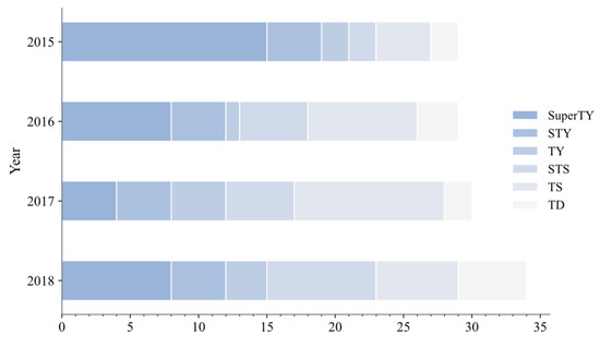
Figure 1.
Information on TCs which arose over the western North Pacific from 2015 to 2018, respectively.
2.2. Prior Physical Factors Related to the TC Intensity
In satellite cloud images, TC intensity is a comprehensive reflection of the cloud’s structure and shape, brightness temperature distribution, and other characteristics (such as the distance between the TC circulation center and the strong convective cloud area, the area of the central strong convective cloud, the outer spiral rain bands, the cloud-top brightness temperature (CTBT) around the TC eye, and the brightness temperature of the eye) [19]. The degree of organization of the TC cloud system and the distance of the deep convection away from the center of the TC reflect the magnitude of the TC vorticity and the magnitude of the vertical wind shear, respectively [20]. The area of the central strong convective cloud, cloud types, and the brightness temperature of the eye all reflect the intensity of deep convection development and the intensity of the TC inner-core development, which are closely related to the changes in TC intensity. A series of studies on infrared cloud images have shown that the distribution of the radiation brightness temperature detected in the infrared channel by geostationary satellites has a strong correlation with TC intensity [21,22,23]. Thus, 14 factors of prior physical factors (Table 2) were selected here to construct the detecting model.
Table 2.
Description of the prior physical factors of the TC intensity.
The morphological structure of TCs (including the degree of organization of the eyewall and the helicity of the spiral rain bands) varies greatly between development stages. For an ideal vortex, the convective intensity increases from the periphery to the center of the circulation, which manifests as the continuous decrease in the brightness temperature from the outside to the eyewall, namely, the directions of the brightness temperature gradient convergently pointing towards the center [13].
The first six factors in Table 2 are related to the deviation angle variance (DAV), which was proposed by Piñeros et al. [8] to describe the degree of axisymmetry of the TC system with cloud images. To calculate the DAV value of a point , a radius should be pre-defined to determine the calculation area. For every point inside the area, the deviation angle is defined as the angle between the bright temperature gradient and its radial direction to the calculation point (shown in Figure 2). Then, the DAV value of can be obtained by calculating the variance of all the deviation angles. Finally, the DAV value at every pixel point constitutes the DAV map. The DAV map can quantify the deviation of the TC system to the ideal vortex. As illustrated in Figure 2, the DAV value of the ideal vortex should be zero at the center and increase radially. It can be seen how the DAV value is negatively proportional to the degree of axisymmetry of the TC system. The smaller the DAV value of a certain reference point is, the greater the degree of axisymmetry of the whole system. In contrast, as the dispersion of the brightness temperature gradient direction increases, the DAV value increases, which is a feature of underdeveloped clouds or TCs in the asymmetric dissipation process. The detailed process of the DAV calculation process can be found in [24].
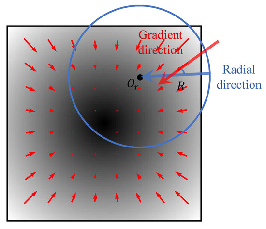
Figure 2.
Schematic of the deviation angle calculation process with the brightness temperature image of an ideal vortex (shaded) and gradient vectors (red).
The calculation radius R was chosen as 300 km based on the research of correlation analysis between the DAV and the TC intensity in WNP [25]. Additionally, according to the research of Yuan and Zhong [20], the threshold DAV value of the organizational cloud cluster of TC is about 2400 deg2 with the FY data in WNP, meaning that the pixels of the DAV map that exceed the threshold should be excluded from the TC area. Compared to previous studies [13,20,24], in which the factor is calculated with a fixed radius, this threshold enables the actual average range to consider the size of the TC. Moreover, we further included the area and ellipticity of the clouds to better reflect the structure of the TCs [26]. Specifically, TC size increases with increasing intensity, but then remains nearly constant or even slowly decreases afterwards [27]. Based on these studies, this paper includes the following factors (1–6) to measure the TC morphological structure:
- (1)
- CoreDAV—the DAV value of the TC center;
- (2)
- MMV—the minimum value of the DAV map, representing the maximum degree of axisymmetry of the cloud within the cloud image at a certain moment;
- (3)
- RD—the relative distance between the MMV position and the TC center. According to Yuan and Zhong [20], the MMV value decreases continuously with increasing TC intensity and gradually moves closer to the center of circulation. A smaller RD value indicates that the MMV position is closer to the TC center, indicating a higher degree of axisymmetry of the TC;
- (4)
- DAVmean— the average DAV value within the cloud with DAV < 2400 deg2;
- (5)
- S2400—the area of the cloud with DAV < 2400 deg2;
- (6)
- E—the ellipticity of the cloud area of DAV < 2400 deg2.
Fitzpatrick [22] showed that the average brightness temperature within a certain range of the TC circulation center has a strong negative correlation with the TC intensity. In other words, a lower average brightness temperature corresponds to a higher convection intensity and thereby a higher TC intensity. Although the CTBT and the convective updraft do not correspond pixel by pixel in the cloud image due to the eyewall inclination and cirrus outflow, the comprehensive characteristics of the CTBT in the region have a good statistical relationship with the typhoon intensity. Dvorak [3] also found that the internal convection of TCs and the organizational structure of deep convection clouds are closely related to the TC intensity. For example, the disturbance model in the statistical hurricane intensity prediction scheme (SHIPS) introduced a series of factors derived from the brightness temperature, and these factors make the greatest contribution to the model through variance testing [21]. This paper introduces the following factors (7–10) in the SHIPS to reflect deep convection information:
- (7)
- TBBmin—the minimum value of the cloud brightness temperature within 100–300 km from the center of TC circulation;
- (8)
- TBBstd—the standard deviation of the brightness temperature of clouds within 100–300 km of the TC circulation center, which can reflect the brightness temperature gradient in the region to a certain extent;
- (9)
- TBBmean —the average brightness temperature of clouds within 100–300 km of the TC circulation center, reflecting the average intensity of deep convection in clouds in the region;
- (10)
- S20—the area proportion of clouds with a brightness temperature below −20 °C within 50–200 km of the center of the TC circulation.
The background field factors selected in this paper are as follows:
- (11)
- Lat_TC,
- (12)
- Lon_TC,
- (13)
- Lat_MMV, and
- (14)
- Lon_MMV.
Lat_TC and Lon_TC are the latitude and longitude of the TC circulation center, respectively, and Lat_MMV and Lon_MMV are the latitude and longitude of the MMV center, respectively. These factors have a strong correlation with the TC intensity and can reflect the different background field information on the TCs to a certain extent [21]. The location of the TC determines the basic environment field, such as a latitude-dependent sea surface temperature and a spatially-varied atmospheric circulation [28], while the location of the MMV provides additional orientation information of the relative distance between the MMV position and the TC center.
2.3. CatBoost-Based TC Intensity Detecting Model
2.3.1. Model Construction
Using the gradient boosting decision tree (GBDT) framework, CatBoost is a boosting algorithm supporting categorical variables with less parameters and a high accuracy [14]. The basic principle of this algorithm is to produce a weak learner at each iteration and train the learner with the results of the previous round. Within the training process, the aim of this model is to continuously improve the accuracy of the learner by reducing the bias and obtain the final strong learner by the weighted summation of the weak learners from each round.
As there are so many numbers and categories of factors that relate to the TC intensity, and with the interaction between these factors being also uncertain, the following settings were used to optimize the possible gradient bias and prediction shift problems in the GBDT algorithm while constructing the CatBoost-based intensity detecting model (Figure 3).
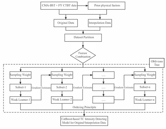
Figure 3.
Process for constructing the CatBoost-based TC intensity detecting model.
- (1)
- The greedy strategy was used for feature combination. The CatBoost algorithm arbitrarily combines categorical features as new features, but if taking all possible combinations into account, the number will explode with the growth of these categorical features. Therefore, we used a greedy strategy to perform a feature combination, that is, when selecting the first segmentation node for the decision tree, any subsequent combination is not considered. In the subsequent division process, the model will combine the category features used by all the segmentation points of the current tree and all the category features in the dataset, and the combined value will be dynamically transformed into numerical features. At the same time, the model will regard all the selected segmentation points in the tree as categorical features with two values and participate in the subsequent feature combination like categorical features;
- (2)
- The ordering principle was used to reduce the gradient deviation and solve the prediction shift problem. In order to obtain an unbiased gradient estimation, a separate learner for each sample was trained with all other data in the training set. Following this, the base learners were continuously trained by calculating the gradient estimate of the sample data to obtain the final model, which can also improve the generalization ability of the model;
- (3)
- The oblivious tree was used for fast scoring. The highest benefit of using the oblivious tree is that the splitting criteria are the same for the internal nodes of the same layer, which means the selected features and feature thresholds at the same split are completely consistent. This means that compared to the general decision tree, the structure of the oblivious tree is more balanced. Using the oblivious tree as the base learner can reduce the possibility of overfitting and improve the processing speed.
2.3.2. Dataset and Evaluation Indices
The essence of the machine learning-based model was to approximate and reproduce the mapping between the input vector and the output vector as accurately as possible. In the TC intensity detecting model, the output vector is the TC intensity described by the maximum surface wind speed at a certain time, while the input vector is the information related to the TC intensity obtained from observations, simulations, or diagnostic analyses, that is, the so-called dataset. In the model construction and analysis, the sample data used for modeling were defined as the training set, and the data used to assess the intensity detecting performance of the model were defined as the testing set, respectively. Random sampling can often yield better model testing results. Therefore, this study employed the random dataset construction method; that is, the processed data and calculated factors in all years were divided randomly at a 4:1 ratio into a training set and a testing set, respectively.
To verify and compare the model’s performance, two types of dataset, the original dataset and the interpolation dataset, were used to take dataset partition and construct the model, respectively. For each type of dataset, the sensitivity test of the model parameters was first performed, and the results under the optimal model parameter configuration were obtained to construct the model. As the dynamic structure and thermal convection of the TC have obvious differences at the different intensity levels, the classification standard of the TC intensity levels (GB/T 19201-2006) was used here to analyze the detecting performance of the model for the seven levels (Table 1).
Following the IR cloud image transformation and factors calculation, 2342 samples were obtained from the original dataset, while 13,471 samples were retrieved from hourly interpolations, respectively. Figure 4 shows the proportion of samples at different TC intensity levels for the original and interpolation dataset, respectively. For the original data, approximately 75% of the TC samples were weaker than the TY, most of which were at the levels of TS and TD, respectively. For the interpolated data, due to the reduction in the time intervals for TC intensity classification, the proportion of high intensity levels above TY was found to have increased, accounting for approximately 30% of all data.
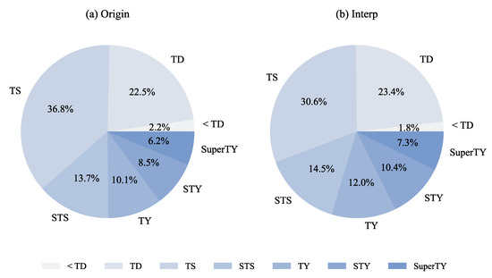
Figure 4.
Proportion of samples of different intensity levels of tropical cyclones in (a) the original dataset and (b) the interpolated dataset.
Two evaluation indices, the root mean square error (RMSE) and R-squared (R2) were selected to evaluate the feasibility and accuracy of the model for the TC intensity detecting model. RMSE is the square root of the ratio of the square of the deviation of the predicted value () from the sample value () to the number of observations (n). RMSE can be calculated as follows:
This index is used to measure the deviation between the predicted value and the sample value. The smaller the RMSE, the more accurately the model can describe with the testing data. RMSE is the most commonly used evaluation index for machine learning-based models, and it is very sensitive to both the large and small errors that may be present in a dataset.
R² can be understood as the goodness-of-fit to a model, and be calculated as:
In which is the mean value of the samples. R2 can reflect how well the regression predictions approximate the samples. Compared with the RMSE, R2 converts the prediction results into accuracy so that the results are all in the interval [0, 1], providing a more intuitive comparison of the different models. Generally, the closer the value is to 1, the better the model fitting effect.
3. Results
3.1. Sensitivity Test of the CatBoost Model’s Hyperparameters
The setting of hyperparameters has a significant impact on the model’s performance. When building a CatBoost model, the main hyperparameters that need to be set include n_estimators, learning_rate, and the depth. N_estimators is the number of decision trees needed for the model’s construction, and the value of n_estimators depends on the specific sample size. An overly large sample size will cause overfitting, while an overly small sample size will result in the failure in obtaining the model features. Learning_rate is the step length of iteration for the gradient reduction, and only affects the training time of the model. The smaller this hyperparameter, the more iterations are required for training. Depth is defined as the tree’s depth. Generally, a greater depth means a better fitting effect, although it increases the computational complexity, slows down the computational speed, and may cause overfitting. As learning_rate has little effect on the final result, its value can be selected to 0.11, according to the performance expectations. In order to evaluate the model’s performance, n_estimators was set to 1000, 2000, 3000, and 4000, while the depth was set to 4, 6, 8, 10, and 12, respectively. Altogether, a total of 20 sets of tests were performed to assess the impact of the hyperparameters of the model on the results from the original and interpolation datasets, respectively.
Figure 5 shows the RMSE of the CatBoost models constructed based on the original data and interpolation data under different hyperparameter schemes. In general, the RMSE showed a trend of decreasing sharply initially and then increasing slowly with depth and n_estimators, indicating that the optimal hyperparameter needs to be a medium value which can control the error without overfitting. In addition, using the interpolation dataset, the RMSE can be reduced to about a third of those with the original dataset, which indicates that improving the temporal resolution of the best-track data and expanding the overall dataset can improve the model’s performance. With either of these two datasets, an n_estimators value of three thousand and a depth of eight was found to give the best results.
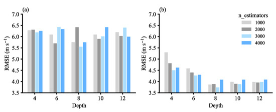
Figure 5.
RMSE of the CatBoost model under different hyperparameter schemes in (a) the original dataset and (b) the interpolation dataset.
3.2. TC Intensity Model Results
3.2.1. Analysis of the Intensity Detecting Results of the Whole Life Cycle
According to the analyses in the previous sections, the CatBoost-based model worked best when the number of decision trees (n_estimators), the learning rate (learning_rate), and the tree depth (depth) were set to 3000, 0.11, and 8, respectively.
Table 3 shows the detecting results of the typhoon intensity using the CatBoost-based models built on the original and interpolated data. All four indices, including the RMSE, R2, and the extremes of deviation between the predictions and the samples, show the better performance of interpolated dataset model than that of the original dataset model. The RMSE of the model trained with the interpolated data was 3.74 m s−1, which was reduced by 33% to those from the original dataset model. Furthermore, the RMSE of this CatBoost-based TC intensity detecting model of the interpolated data was lower than the results in Lee et al. [12] and Zhong et al. [13]. The error extremes, being the max and min deviations of the model trained with the interpolated data were 16% and 9% lower than those of the model trained with the original data, respectively, while the R2 increased from 0.78 to 0.92, respectively. These results indicate that the use of the interpolated dataset not only can optimize the fitting effect of large sample points but can also have a good correction effect on the extreme value errors.
Table 3.
The errors of the CatBoost-based model under different datasets.
Figure 6 shows the scatter distribution and deviation frequency distribution plots of the TC intensities predicted using the CatBoost-based model (V_pred) and TC intensities recorded in the CMA-BST (V_test). The fitting lines of the two types of datasets both rotated in a clockwise direction. That is, when the TC intensity was less than 22 m s−1, the TC intensity detected by the CatBoost-based model was found to be higher than that recorded in the CMA-BST, and it was lower when the TC intensity was greater than 22 m s−1. The CatBoost-based model exhibits the systematic biases of overestimation at a low-level intensity TC and underestimation at a high-level intensity TC. However, the scatter distribution from the different datasets (Figure 6a) show that the interpolated dataset expands the high-intensity TC samples and significantly reduces the deviation to the detecting results above 40 m s−1. The kernel density curve (Figure 6b) of the interpolated data was found to be narrower and taller, and the errors of the interpolated data were concentrated within −2 to 2 m s−1 with a smaller overall variance, whereas the kernel density curve of the original data was wider and shorter, and there were lots of samples located in the area of deviation exceeding −20 m s−1. The above results indicate that the interpolated data can not only improve the performance of the model but can also reduce the variance of the model’s predictions somewhat, thereby making the model more stable.
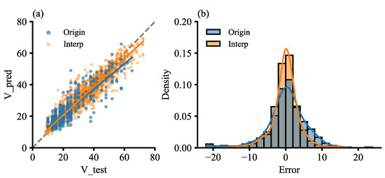
Figure 6.
CatBoost model: (a) scatter plots of the predicted intensities (V_pred) and CMA-BST (V_test). The dashed line is the perfect prediction line y = x and the solid lines are the fitted curves. (b) Deviation frequency distribution plots and superimposed kernel density fitting curves. Blue color represents the results obtained based on the original dataset, and orange represents the results obtained based on the interpolated dataset. The original dataset produces error from −22.01 to 23.96 m s−1, while the interpolated dataset produces error from −20.02 to 19.9 m s−1, respectively.
3.2.2. Detecting Results of TC Intensity at Different Levels
Considering the deviation of the model fitting line from the perfect prediction line, the detecting results of the models at different TCs intensity levels were analyzed.
Figure 7 shows the detecting results of the CatBoost model trained by the original dataset and the CatBoost-based model trained by the interpolated dataset for different TC intensity levels. The errors of the two models have similar trends with increasing TC intensity. Both models demonstrate a good performance for the TS and TD levels, with their RMSE being less than 4 m s−1. For TCs above STS, the intensity estimation errors increased quickly with the TC intensity. In addition, the most obvious accuracy improvements with the interpolated dataset were at the levels of WeakTD and SuperTY. Based on the analysis of the dataset sample distribution in previous sections, it is shown how there is an evident correspondence between the model estimation results and the sample size. The detecting results of the TCs weaker than TS have the largest number of samples and the lowest errors of no more than 3 m s−1. It can also be understood that interpolation, which can expand the sample size, can also significantly reduce the RMSE of the detecting results. Furthermore, this model showed an excellent fitting effect at the level of WeakTD and TD, which overcome the weaknesses of the existing objective models in locating position and estimating the intensity in the early stages of a TC [6,12]. This improvement depends on the prior physical factors used in this paper, which have been investigated to obtain a good description ability to the TC structure at its early stage.
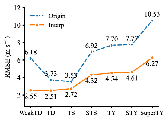
Figure 7.
RMSE of the CatBoost-based model for tropical cyclones (TCs) of different intensity levels with the original dataset (blue dashed line) and the interpolated dataset (orange solid line).
Figure 8 shows the distribution of deviations of the CatBoost-based model results from the CMA-BST data at different levels of TC intensity. The median intensity deviation of the model was close to the zero-value line at the levels of TD, TS, and STS. The deviation observed was clearly positive at low-intensity levels, while markedly negative at levels above TY. Overall, this CatBoost-based model appears to have the problem of overestimating at low intensities and underestimating at high intensities. Furthermore, the boxes obtained using the model trained on the original data deviated more in length (spread) and position than those obtained with the model trained on the interpolated data, which further shows that using the interpolated data to train the model can reduce the deviation and variance of the model and thereby improve the accuracy of the model.
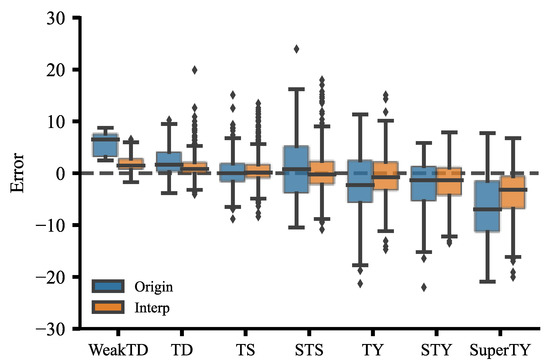
Figure 8.
Boxplots of the distribution of the deviations of the CatBoost model results from the CMA-BST data at different intensity levels. The box extends from the first quartile to the third quartile of the error, with a line at the median. The whiskers extend from the box by 1.5× the interquartile range. Outlier points are those past the end of the whiskers.
At each TC intensity level, the CatBoost model trained on the interpolated data performed the best and produced results better compared to the three other results. The CatBoost model encompasses the same systematic biases of overestimation at low intensities and underestimation at high intensities. On the one hand, this was deemed to be due to the influence of sample size. On the other hand, the prior factors of the model were not discriminative enough in their quantitative description of high-intensity TCs. The reason for this may be that when a TC is enhanced, its potential temperature gradient information is possibly masked due to the limited resolution of the satellite, resulting in underestimation at high intensities. Furthermore the poor time resolution of the best-track data may also attribute to the bias of the model. In reality, the intensity of a TC changes in high frequency, while the linear interpolation is impossible to reproduce the fluctuations and tends to underestimate the true intensity.
3.3. Detecting Test of the Model with Independent and Individual TCs
The objective and quantitative detecting of TC intensity is an urgent need for operational typhoon forecasting. To assess the real-time detecting performance and generalization ability of the model for unseen and individual TCs, this paper used the CatBoost-based optimization model, which was constructed based on random datasets to estimate the intensities of TCs from 2019 and of two individual TCs, including the No. 29 STY Phanfone (1223 UTC 12-1228 UTC 03) in 2019 and the No. 9 super TY Maysak (0828 UTC 09-0903 UTC 18) in 2020, which were all not included in the training and testing process.
According to the CMA-best-track data, there are 29 named TCs developed in the WNP in 2019 with a total of 529 times. Figure 9 shows the validation results of all 29 named TCs in 2019. The intensities of most cases are well replicated except for the No. 20 and No. 23 cases. These two cases both showed rapid intensification and rapid weakening, with their strongest intensity lasting for a very short time. Therefore, it is rather difficult for the model to capture the intensity of these two TCs. The total RMSE was 4.90 m s−1, which was still deemed to be competitive compared with other models, indicating that our model is robust and can be generalized to estimate the intensity for future TCs.
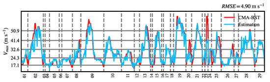
Figure 9.
Comparison of the estimation of our model with CMA best-track data in 2019. The red line indicates the intensity from CMA best-track while the blue line shows the results of our model.
Phanfone was a severe typhoon in 2019 with a typical westward track. The intensity evolution and model detecting results of Phanfone is demonstrated in Figure 10. The mean average error of the model for Phanfone was 1.09 m s−1, showing a great performance of the model in estimating the intensities. Even though the maximum wind speed of Phanfone reached 42 m s−1, a level at which the model typically shows a great underestimation, the value and trend of its intensity evolution were still accurately reproduced.
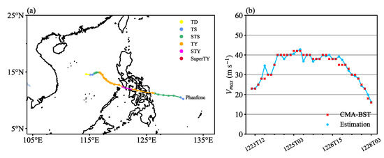
Figure 10.
(a) Track and intensity of Phanfone. (b) Time series of its intensity, as predicted using the model (blue) and as recorded in CMA-BST (red). The study time was 1223 UTC 12-1228 UTC 03, and the temporal resolution was 3 h. The case was affected by the cold air and therefore weakened and disappeared in the center of the South China Sea.
Maysak was one of the strongest typhoons in 2020, with another typical northward track, and which later turned into an extratropical cyclone. Figure 11 shows the basic evolution of Maysak and compares the model detecting results and the CMA-BST data. The intensity prediction error of the model for Maysak was 5.66 m s−1, which indicates that the model also exhibits a good intensity prediction performance for SuperTYs. The model reproduces its intensifying and weakening trends well, and the maximum intensity predicted by the model is consistent with that recorded in the CMA-BST, although the model overestimates the intensity of Maysak during its rapid intensification phase. The overestimation might attribute to the eyewall replacement cycle, which have been frequently observed in intense TCs [29]. During rapid intensification, the main eyewall contracts are gradually replaced by the secondary eyewall [30]. Therefore, this cycle can clearly affect the calculation of the physical factors and subsequently impact the performance of the model, which can be evidenced by the apparent fluctuations of the predicted intensity evolution. Linear interpolation of the best-track data is obviously unable to reproduce the real-time series, and therefore the mismatch in the temporal resolution between the physical factors and the best-track data might also have impacts on the model’s performance. After Maysak turned into an extratropical cyclone (0903T00) in the late stage, the model still accurately estimates its intensity. Interestingly, the model exhibits an opposite performance with an overestimate in the intensifying period and an underestimate in the decaying period even if Maysak has the same intensity, indicating that these evolution trends are probably helpful in detecting the TC intensity.
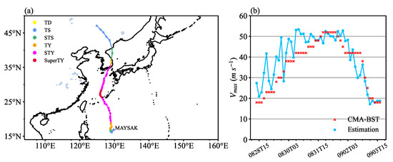
Figure 11.
Same as Figure 9, except in that the study time is 0828 UTC 15-0903 UTC 15 for Maysak (a,b).
Overall, the model distinguishes the TC intensities well and performs best at a TC intensity of about 20 m s−1. In the analyses in previous sections, the model error mainly manifested as underestimation at high intensities and overestimation at low intensities. However, the STY Phanfone was well detected, while the intensity of Maysak was overestimated, indicating that the strengthening processes of Phanfone and Maysak are quite different, and that there are probably other factors are relevant to the intensity of TCs. Why the model performs differently for these two typhoons requires further study.
4. Summary
In this paper, the CatBoost-based model was used to construct an objective TC intensity-detecting model based on IR cloud image data. An original dataset and an interpolated dataset were used by considering the different resolutions of the source datasets. The intensity prediction performances of the CatBoost-based model in different datasets and for different TC intensity levels were comparatively analyzed. The following main conclusions are drawn:
- (1)
- After data interpolation to further expand the dataset size, the RMSE of the CatBoost model was further reduced, the error distribution was more concentrated, the deviation and variance of the model were reduced, and the performance of the model was enhanced;
- (2)
- Compared with the RMSE of 4.27 m s−1 of the pure CNN models, which has shown the best performance to our knowledge so far [12], the CatBoost-based model based on prior physical factors has smaller errors (a RMSE of 3.74 m s−1) in detecting the TC intensity and has a better intensity prediction performance;
- (3)
- The CatBoost-based model has systematic biases of overestimation at low intensities and underestimation at high intensities, and the intensity estimation deviation may be larger for the high-intensity or rapid intensification TCs.
In order to further improve the accuracy for intensity detection oversea, more data sources and more high-correlation prior physical factors should be used. The expansion of the data source can reduce or eliminate the underestimation of high-intensity TCs caused by the gradient vanishing problem of the IR images. Moreover, finding and using more high-correlation prior physical factors can further enhance the understandability of the deep learning model and specifically improve the model’s accuracy.
Author Contributions
Conceptualization, methodology, W.Z. and Y.S.; Software, formal analysis, investigation, W.Z. and D.Z.; validation, resources and data curation Q.W., W.Z. and D.Z.; writing—original draft preparation, W.Z. and D.Z.; writing—review and editing, Y.S. All authors have read and agreed to the published version of the manuscript.
Funding
This research was funded by the General Program of National Natural Science Foundation of China (No. 42075011, 42075035) and the Major Research Plan of National Natural Science Foundation of China (No. 42192552).
Data Availability Statement
The satellite data used in this study can be downloaded at https://satellite.nsmc.org.cn/portalsite/Data/Satellite.aspx (accessed on 10 July 2023). The best-track data from the China Meteorological Administration is available at https://tcdata.typhoon.org.cn/zjljsjj_zlhq.html (accessed on 10 July 2023). The CatBoost algorithm is in open-source and can be obtained at https://catboost.ai (accessed on 10 July 2023). All figures in the paper are generated by the Matplotlib library in Python 3.7 (https://matplotlib.org/, accessed on 10 July 2023).
Conflicts of Interest
The authors declare no conflict of interest.
References
- Camargo, S.J.; Sobel, A.H. Western North Pacific Tropical Cyclone Intensity and ENSO. J. Clim. 2005, 18, 2996–3006. [Google Scholar] [CrossRef]
- Harnos, D.S.; Nesbitt, S.W. Convective structure in rapidly intensifying tropical cyclones as depicted by passive microwave measurements. Geophys. Res. Lett. 2011, 38, 1451–1453. [Google Scholar] [CrossRef]
- Dvorak, V.F. Tropical Cyclone Intensity Analysis and Forecasting from Satellite Imagery. Mon. Weather Rev. 1975, 103, 420–430. [Google Scholar] [CrossRef]
- Olander, T.L.; Velden, C.S. The Advanced Dvorak Technique: Continued Development of an Objective Scheme to Estimate Tropical Cyclone Intensity Using Geostationary Infrared Satellite Imagery. Weather Forecast. 2007, 22, 287–298. [Google Scholar] [CrossRef]
- Velden, C.S.; Hayden, C.M.; Nieman, S.J.W.; Menzel, W.P.; Wanzong, S.; Goerss, J.S. Upper-Tropospheric Winds Derived from Geostationary Satellite Water Vapor Observations. Bull. Am. Meteorol. Soc. 1997, 78, 173–196. [Google Scholar] [CrossRef]
- Engel, G. Satellite Applications at the Joint Typhoon Warning Center. In Proceedings of the 5th WMO International Workshop on Tropical Cyclones, Cairns, Australia, 3–12 December 2002; WMO: Geneva, Switzerland, 2002. [Google Scholar]
- Knaff, J.A.; Brown, D.P.; Courtney, J.; Gallina, G.M.; Beven, J.L. An Evaluation of Dvorak Technique–Based Tropical Cyclone Intensity Estimates. Weather Forecast. 2010, 25, 1362–1379. [Google Scholar] [CrossRef]
- Piñeros, M.F.; Ritchie, E.A.; Tyo, J.S. Objective Measures of Tropical Cyclone Structure and Intensity Change from Remotely Sensed Infrared Image Data. IEEE Trans. Geosci. Electron. 2008, 46, 3574–3580. [Google Scholar] [CrossRef]
- Piñeros, M.F.; Ritchie, E.A.; Tyo, J.S. Estimating Tropical Cyclone Intensity from Infrared Image Data. Weather Forecast. 2011, 26, 690–698. [Google Scholar] [CrossRef]
- Zhang, C.; Qian, J.; Ma, L.; Lu, X. Tropical Cyclone Intensity Estimation Using RVM and DADI Based on Infrared Brightness Temperature. Weather Forecast. 2016, 31, 1643–1654. [Google Scholar] [CrossRef]
- Pradhan, R.; Aygun, R.S.; Maskey, M.; Ramachandran, R.; Cecil, D.J. Tropical Cyclone Intensity Estimation Using a Deep Convolutional Neural Network. IEEE Trans. Image Process. 2018, 27, 692–702. [Google Scholar] [CrossRef]
- Lee, J.; Im, J.; Cha, D.-H.; Park, H.; Sim, S. Tropical Cyclone Intensity Estimation Using Multi-Dimensional Convolutional Neural Networks from Geostationary Satellite Data. Remote Sens. 2020, 12, 108. [Google Scholar] [CrossRef]
- Zhong, W.; Yuan, M.; Ye, H.; Luo, X. 2020: Multi-Factor Intensity Estimation for Tropical Cyclones in the Western North Pacific Based on the Deviation Angle Variance Technique. J. Meteorol. Res. 2020, 34, 1038–1051. [Google Scholar] [CrossRef]
- Prokhorenkova, L.; Gusev, G.; Vorobev, A.; Dorogush, A.V.; Gulin, A. CatBoost: Unbiased boosting with categorical features. In Proceedings of the 32nd International Conference on Neural Information Processing Systems (NIPS’18), Montréal, QC, Canada, 3–8 December 2018; Curran Associates Inc.: Red Hook, NY, USA, 2018; pp. 6639–6649. [Google Scholar]
- Qian, Q.; Jia, X.; Lin, H.; Zhang, R. Seasonal Forecast of Nonmonsoonal Winter Precipitation over the Eurasian Continent Using Machine-Learning Models. J. Clim. 2021, 34, 7113–7129. [Google Scholar]
- Zhang, Y.; Ye, A. Machine Learning for Precipitation Forecasts Postprocessing: Multimodel Comparison and Experimental Investigation. J. Hydrometeor. 2021, 22, 3065–3085. [Google Scholar]
- Wu, H.; Yong, B.; Shen, Z.; Qi, W. Comprehensive error analysis of satellite precipitation estimates based on Fengyun-2 and GPM over Chinese mainland. Atmos. Res. 2021, 263, 105805. [Google Scholar] [CrossRef]
- Ying, M.; Zhang, W.; Yu, H.; Lu, X.; Feng, J.; Fan, Y.; Zhu, Y.; Chen, D. An Overview of the China Meteorological Administration Tropical Cyclone Database. J. Atmos. Ocean Technol. 2014, 31, 287–301. [Google Scholar] [CrossRef]
- Velden, C.; Harper, B.; Wells, F.; Beven, J.L.; Zehr, R.; Olander, T.; Mayfield, M.; Guard, C.; Lander, M.; Edson, R.; et al. Supplement To: The Dvorak Tropical Cyclone Intensity Estimation Technique: A Satellite-Based Method that Has Endured for over 30 Years. Bull. Am. Meteorol. Soc. 2006, 87, S6–S9. [Google Scholar] [CrossRef]
- Yuan, M.; Zhong, W. Detecting intensity evolution of the western North Pacific super typhoons in 2016 using the deviation angle variance technique with FY data. J. Meteor. Res. 2019, 33, 104–114. [Google Scholar] [CrossRef]
- DeMaria, M.; Kaplan, J. A Statistical Hurricane Intensity Prediction Scheme (SHIPS) for the Atlantic Basin. Weather Forecast. 1994, 9, 209–220. [Google Scholar] [CrossRef]
- Fitzpatrick, P.J. Understanding and Forecasting Tropical Cyclone Intensity Change with the Typhoon Intensity Prediction Scheme (TIPS). Weather Forecast. 1997, 12, 826–846. [Google Scholar] [CrossRef]
- Gentry, R.C.; Rodgers, E.; Steranka, J.; Shenk, W.E. Predicting Tropical Cyclone Intensity Using Satellite-Measured Equivalent Blackbody Temperatures of Cloud Tops. Mon. Weather Rev. 1980, 108, 445–455. [Google Scholar] [CrossRef]
- Piñeros, M.F.; Ritchie, E.A.; Tyo, J.S. Detecting Tropical Cyclone Genesis from Remotely Sensed Infrared Image Data. IEEE Geosci. Remote Sens. Lett. 2010, 7, 826–830. [Google Scholar] [CrossRef]
- Ritchie, E.A.; Wood, K.M.; Rodríguez-Herrera, O.G.; Piñeros, M.F.; Tyo, J.S. Satellite-Derived Tropical Cyclone Intensity in the North Pacific Ocean Using the Deviation-Angle Variance Technique. Weather Forecast. 2014, 29, 505–516. [Google Scholar] [CrossRef]
- Wang, Y. Recent research progress on tropical cyclone structure and intensity. Trop. Cyclone Res. Rev. 2012, 1, 254–275. [Google Scholar]
- Sun, J.; Cai, M.; Liu, G.; Yan, R.; Zhang, D. Uncovering the Intrinsic Intensity–Size Relationship of Tropical Cyclones. J. Atmos. Sci. 2022, 79, 2881–2900. [Google Scholar] [CrossRef]
- Kossin, J.P.; Knaff, J.A.; Berger, H.I.; Herndon, D.C.; Cram, T.A.; Velden, C.S.; Murnane, R.J.; Hawkins, J.D. Estimating hurricane wind structure in the absence of aircraft reconnaissance. Weather Forecast. 2007, 22, 89–101. [Google Scholar] [CrossRef]
- Sitkowski, M.; Kossin, J.P.; Rozoff, C.M. Intensity and structure changes during hurricane eyewall replacement cycles. Mon. Weather Rev. 2011, 139, 3829–3847. [Google Scholar] [CrossRef]
- Lin, I.-I.; Rogers, R.F.; Huang, H.-C.; Liao, Y.-C.; Herndon, D.; Yu, J.-Y.; Chang, Y.-T.; Zhang, J.A.; Patricola, C.M.; Pun, I.-F.; et al. A Tale of Two Rapidly Intensifying Supertyphoons: Hagibis (2019) and Haiyan (2013). Bull. Am. Meteorol. Soc. 2021, 102, E1645–E1664. [Google Scholar] [CrossRef]
Disclaimer/Publisher’s Note: The statements, opinions and data contained in all publications are solely those of the individual author(s) and contributor(s) and not of MDPI and/or the editor(s). MDPI and/or the editor(s) disclaim responsibility for any injury to people or property resulting from any ideas, methods, instructions or products referred to in the content. |
© 2023 by the authors. Licensee MDPI, Basel, Switzerland. This article is an open access article distributed under the terms and conditions of the Creative Commons Attribution (CC BY) license (https://creativecommons.org/licenses/by/4.0/).