


Sentinel-1 Time Series for Predicting Growing Stock Volume of Boreal Forest: Multitemporal Analysis and Feature Selection

 ,
,  ,
, 
Abstract
1. Introduction
Goals and Contributions of This Study
2. Materials
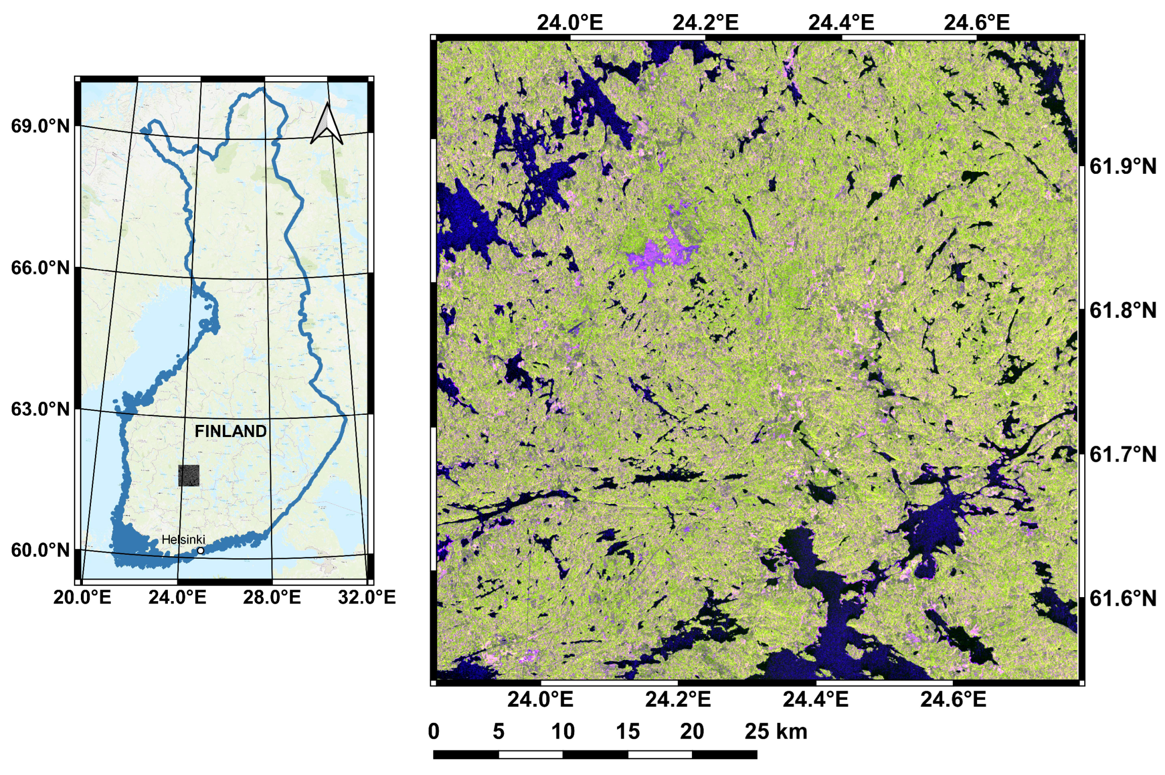
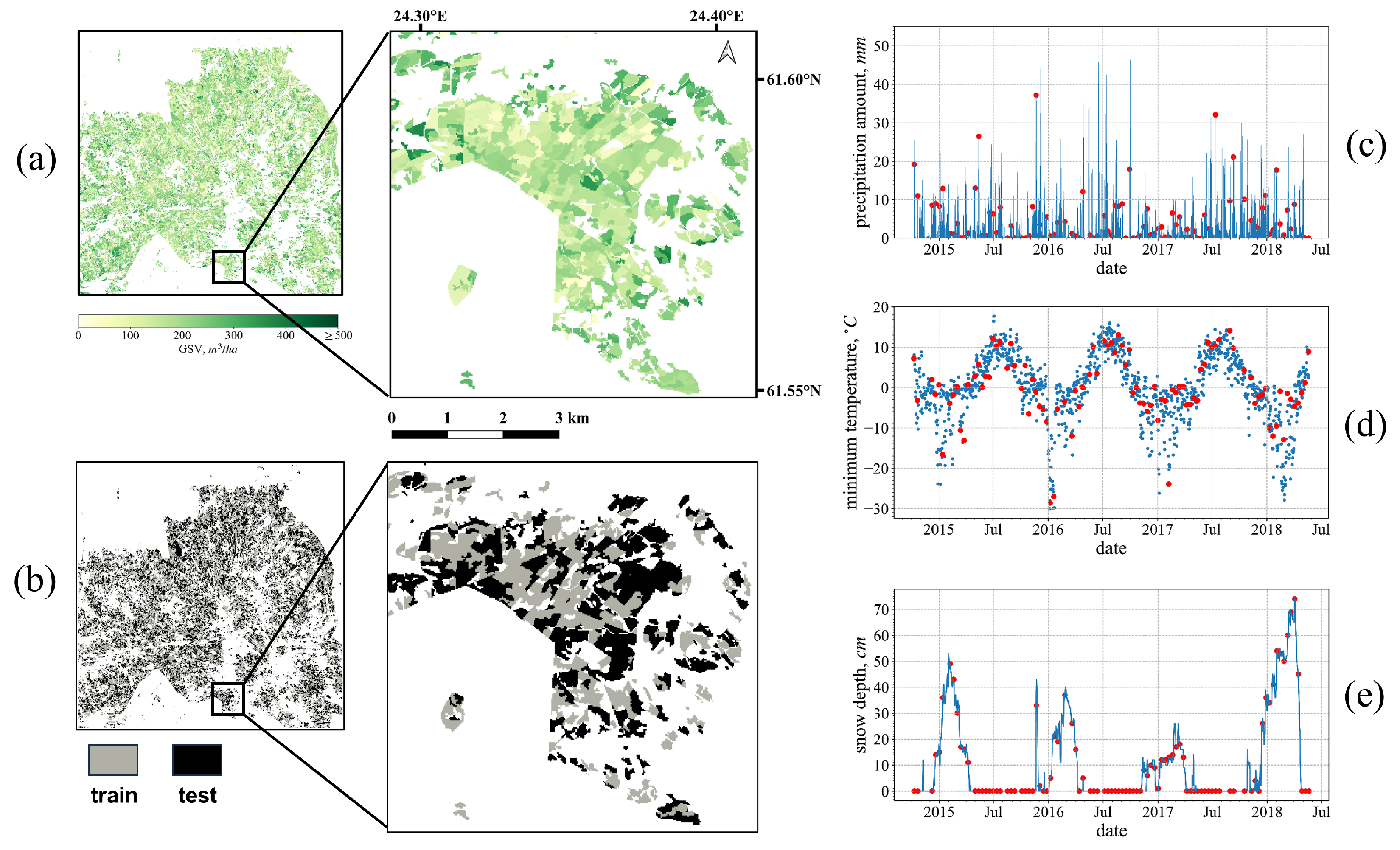
2.1. Study Site
2.2. Sentinel-1 Data
2.3. Ground Reference Data
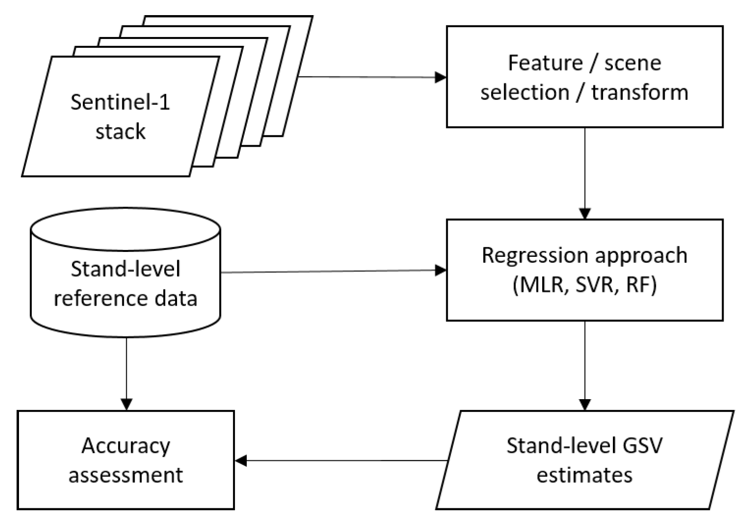
3. Methodology
3.1. Methods for Predicting Growing Stock Volume
3.1.1. Multiple Linear Regression
3.1.2. Support Vector Regression
3.1.3. Random Forests
3.2. Feature Transformation and Selection
3.2.1. Principal Component Analysis
3.2.2. Feature Selection Using Radiometric Contrast
3.2.3. Feature Selection Using Mutual Information
3.2.4. Feature Selection Using Lasso
3.2.5. Feature Selection Using ik-NN
- is the standard error of the prediction of the forest variable r at the stand level,
- is the mean deviation of the forest variable r at the stand level,
- the number of the forest variables used in the algorithm (here, one variable),
- and are fixed constant vectors.
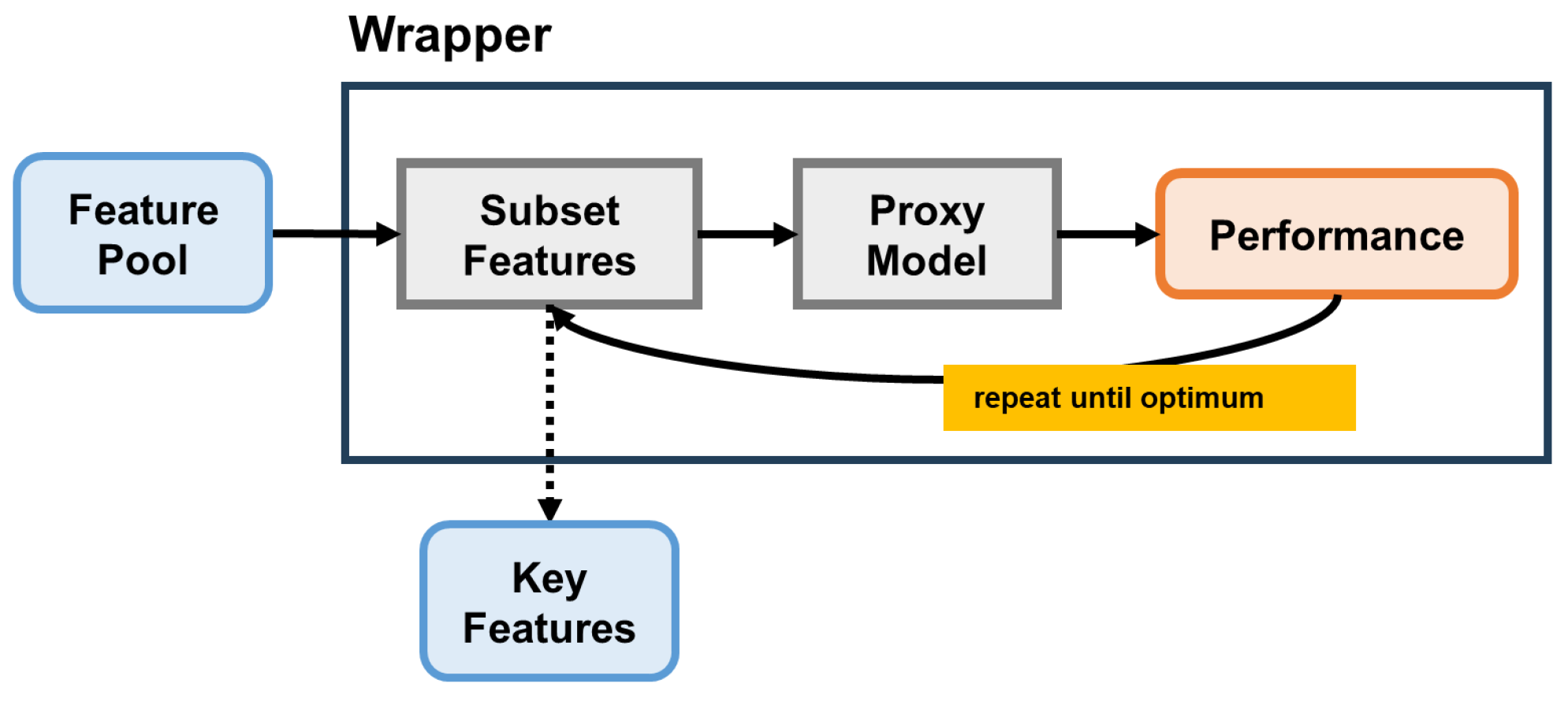
3.2.6. Feature Selection Using Wrapper Methods
3.3. Multitemporal Analysis Using “Sliding Window”
4. Results
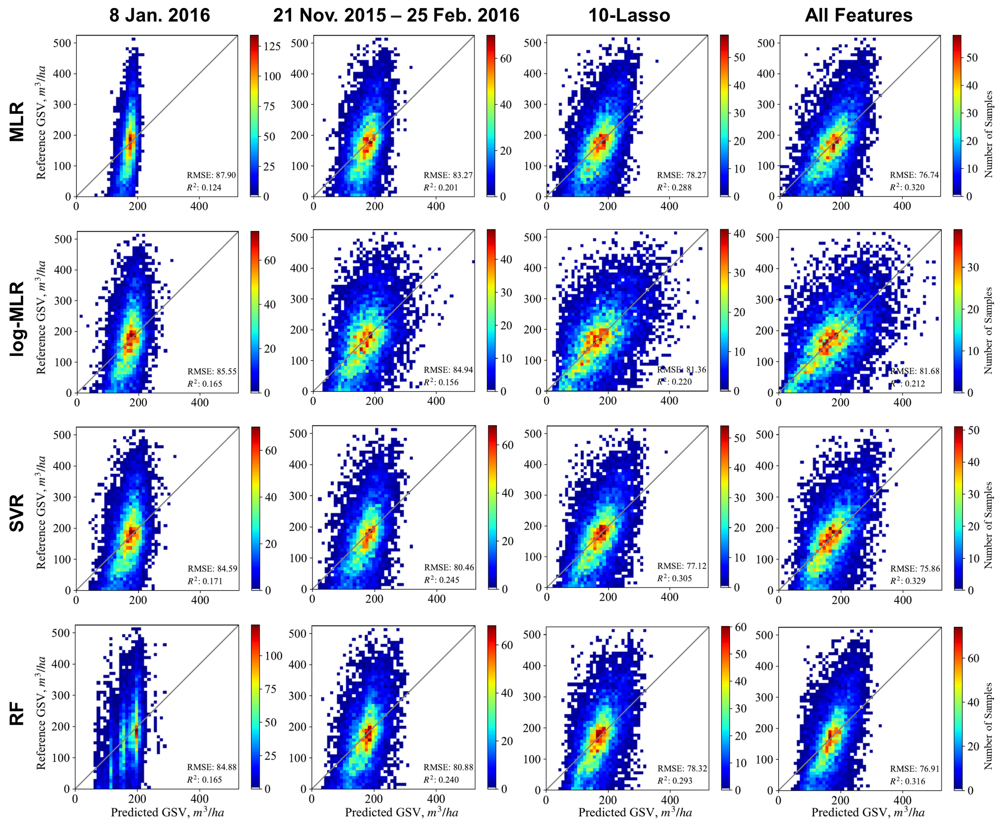
4.1. Accuracy of GSV Prediction
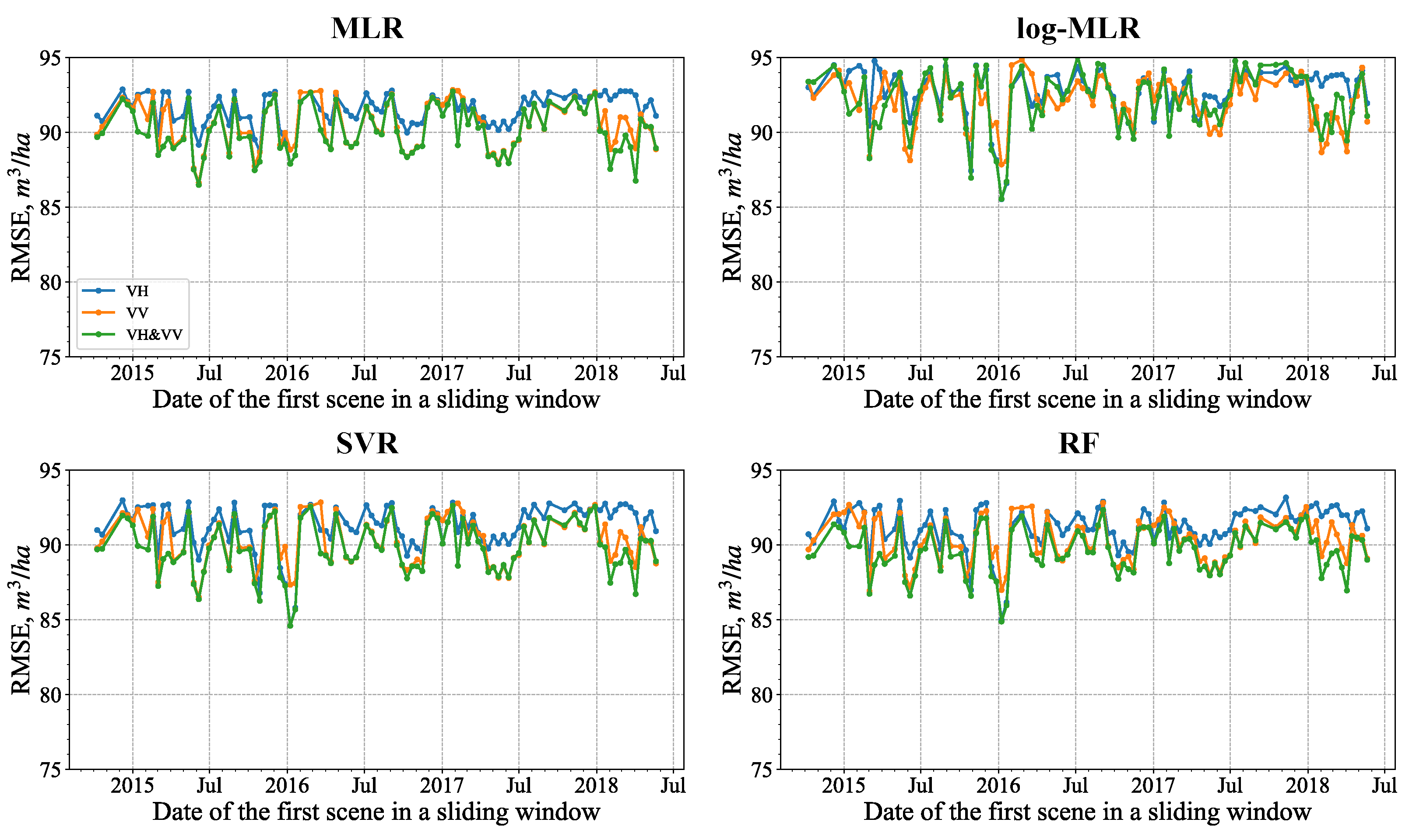
4.1.1. Single SAR Images and Seasonal Variation of the Predictions
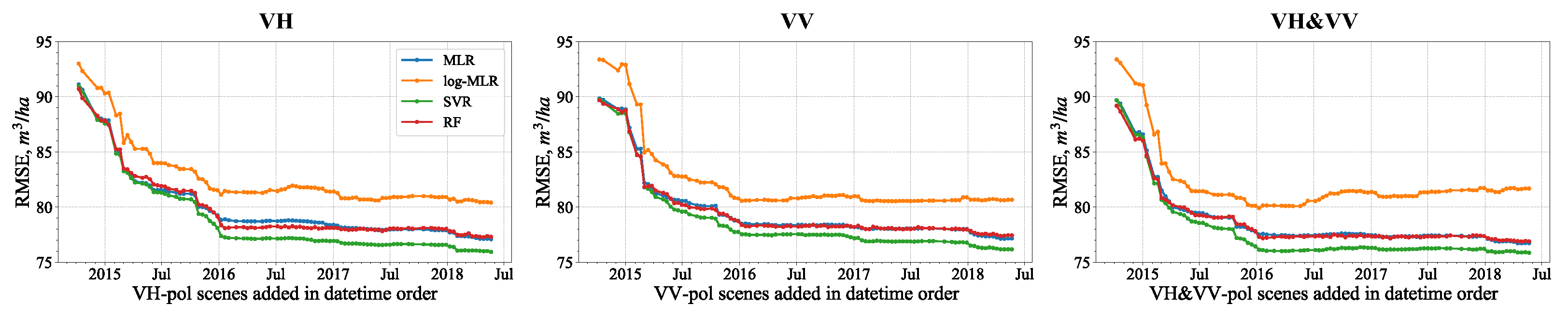
4.1.2. Accumulated SAR Time Series
4.2. Feature Selection
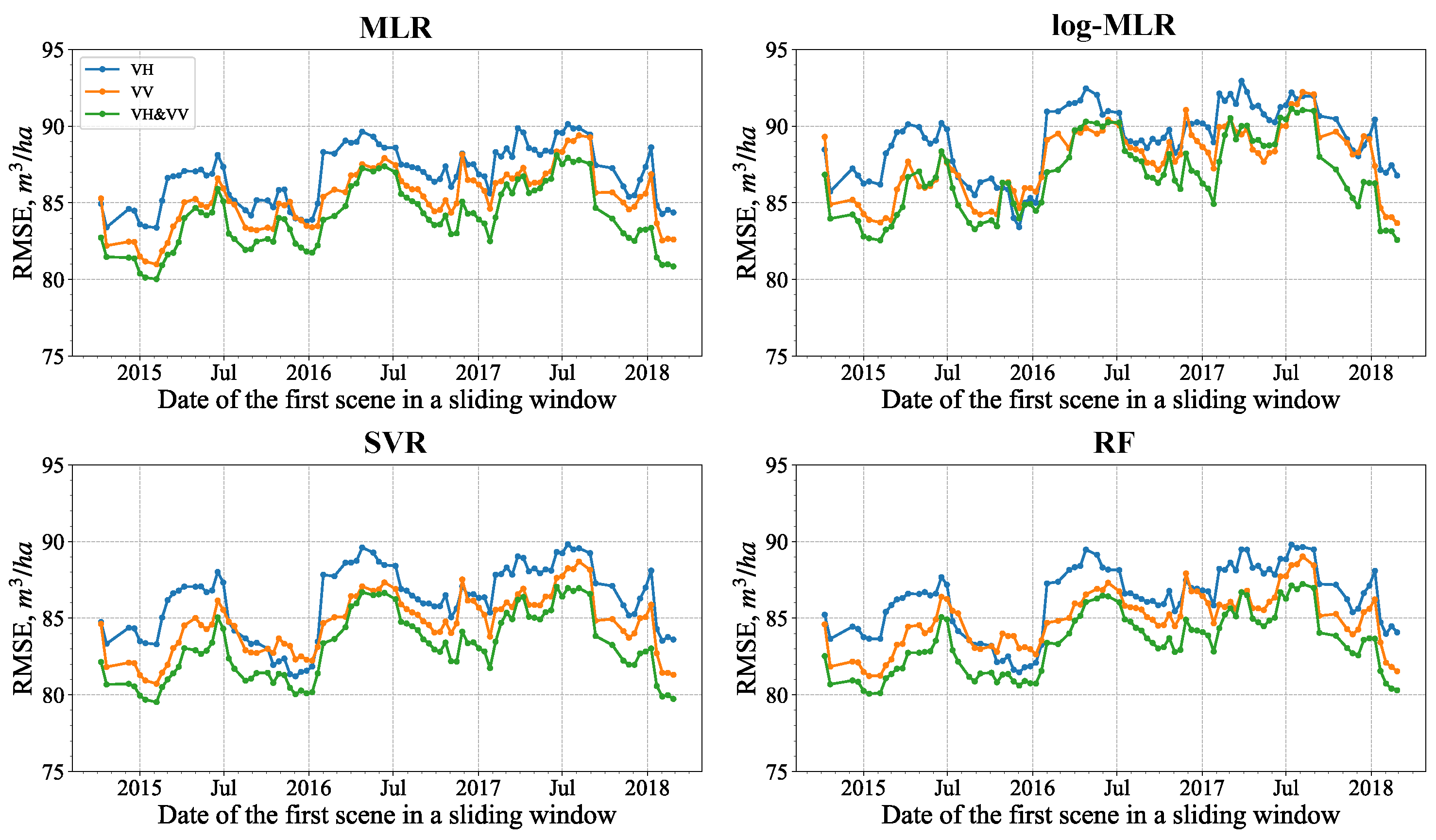
4.3. Sliding Window Analysis
Different Regressions over an Eight-Image Sliding Window
5. Discussion
5.1. On GSV Prediction Methods
5.2. The Effects of Seasonality on GSV Prediction
5.3. Comparison with Previous Studies in Terms of GSV Accuracy and Unit Size
6. Conclusions
Author Contributions
Funding
Conflicts of Interest
Abbreviations
| AGB | above-ground tree biomass |
| ALS | airborne laser scanning |
| CART | classification and regression trees |
| DEM | digital elevation model |
| ESA | European Space Agency |
| GRDH | ground-range detected high-resolution |
| GSV | growing stock volume |
| ik-NN | improved k-nearest neighbors |
| IW | interferometric wideswath |
| Lasso | least absolute shrinkage and selection operator |
| LSE | least squares estimation |
| MAE | mean absolute error |
| MI | mutual information |
| MLR | multiple linear regression |
| MSE | mean squared error |
| OOB | out-of-bag |
| PCA | principal component analysis |
| RBF | radial basis function |
| RC | radiometric contrast |
| RF | random forests |
| RF-Sel | random forests selection |
| RMSE | root mean squared error |
| rRMSE | relative root mean squared error |
| SAR | synthetic aperture radar |
| SFS | sequential feature selection |
| SVR | support vector regression |
| SVM | support vector machines |
| WCM | water cloud model |
References
- Rosenqvist, A.; De Grandi, G.; Rauste, Y.; Shimada, M.; Chapman, B.; Shimada, A.; Saatchi, S. The global rain forest mapping project a review. Int. J. Remote Sens. 2000, 21, 1375–1387. [Google Scholar] [CrossRef]
- Wagner, W.; Luckman, A.; Vietmeier, J.; Tansey, K.; Balzter, H.; Schmullius, C.; Davidson, M.; Gaveau, D.; Gluck, M.; Le Toan, T.; et al. Large-scale mapping of boreal forest in SIBERIA using ERS tandem coherence and JERS backscatter data. Remote Sens. Environ. 2003, 85, 125–144. [Google Scholar] [CrossRef]
- Rodríguez-Veiga, P.; Quegan, S.; Carreiras, J.; Persson, H.; Fransson, J.; Hoscilo, A.; Ziółkowski, D.; Stereńczak, K.; Lohberger, S.; Stängel, M.; et al. Forest biomass retrieval approaches from earth observation in different biomes. Int. J. Appl. Earth Obs. Geoinf. 2019, 77, 53–68. [Google Scholar] [CrossRef]
- Sinha, S.; Jeganathan, C.; Sharma, L.K.; Nathawat, M.S. A review of radar remote sensing for biomass estimation. Int. J. Environ. Sci. Technol. 2015, 12, 1779–1792. [Google Scholar] [CrossRef]
- Global Forest Observations Initiative. Integrating Remote-Sensing and Ground-Based Observations for Estimation of Emissions and Removals of Greenhouse Gases in Forests: Methods and Guidance from the Global Forest Observations Initiative; Group on Earth Observations: Geneva, Switzerland, 2014. [Google Scholar]
- Sarker, M.L.R.; Nichol, J.; Iz, H.B.; Ahmad, B.B.; Rahman, A.A. Forest Biomass Estimation Using Texture Measurements of High-Resolution Dual-Polarization C-band SAR Data. IEEE Trans. Geosci. Remote Sens. 2013, 51, 3371–3384. [Google Scholar] [CrossRef]
- Bourgoin, C.; Blanc, L.; Bailly, J.S.; Cornu, G.; Berenguer, E.; Oszwald, J.; Tritsch, I.; Laurent, F.; Hasan, A.F.; Sist, P.; et al. The Potential of Multisource Remote Sensing for Mapping the Biomass of a Degraded Amazonian Forest. Forests 2018, 9, 303. [Google Scholar] [CrossRef]
- Chen, L.; Wang, Y.; Ren, C.; Zhang, B.; Wang, Z. Optimal Combination of Predictors and Algorithms for Forest Above-Ground Biomass Mapping from Sentinel and SRTM Data. Remote Sens. 2019, 11, 414. [Google Scholar] [CrossRef]
- Reis, A.A.D.; Franklin, S.E.; de Mello, J.M.; Junior, F.W.A. Volume estimation in a Eucalyptus plantation using multi-source remote sensing and digital terrain data: A case study in Minas Gerais State, Brazil. Int. J. Remote Sens. 2019, 40, 2683–2702. [Google Scholar] [CrossRef]
- Tomppo, E.; Antropov, O.; Praks, J. Boreal Forest Snow Damage Mapping Using Multi-Temporal Sentinel-1 Data. Remote Sens. 2019, 11, 384. [Google Scholar] [CrossRef]
- Torres, R.; Snoeij, P.; Geudtner, D.; Bibby, D.; Davidson, M.; Attema, E.; Potin, P.; Rommen, B.; Floury, N.; Brown, M.; et al. GMES Sentinel-1 mission. Remote Sens. Environ. 2012, 120, 9–24. [Google Scholar] [CrossRef]
- Kurvonen, L.; Pulliainen, J.; Hallikainen, M. Retrieval of biomass in boreal forests from multitemporal ERS-1 and JERS-1 SAR images. IEEE Trans. Geosci. Remote Sens. 1999, 37, 198–205. [Google Scholar] [CrossRef]
- Santoro, M.; Beer, C.; Cartus, O.; Schmullius, C.; Shvidenko, A.; McCallum, I.; Wegmüller, U.; Wiesmann, A. Retrieval of growing stock volume in boreal forest using hyper-temporal series of Envisat ASAR ScanSAR backscatter measurements. Remote Sens. Environ. 2011, 115, 490–507. [Google Scholar] [CrossRef]
- Pulliainen, J.T.; Kurvonen, L.; Hallikainen, M.T. Multitemporal behavior of L- and C-band SAR observations of boreal forests. IEEE Trans. Geosci. Remote Sens. 1999, 37, 927–937. [Google Scholar] [CrossRef]
- Rauste, Y. Multi-temporal JERS SAR data in boreal forest biomass mapping. Remote Sens. Environ. 2005, 97, 263–275. [Google Scholar] [CrossRef]
- Santoro, M.; Eriksson, L.; Askne, J.; Schmullius, C. Assessment of stand-wise stem volume retrieval in boreal forest from JERS-1 L-band SAR backscatter. Int. J. Remote Sens. 2006, 27, 3425–3454. [Google Scholar] [CrossRef]
- Cartus, O.; Santoro, M.; Kellndorfer, J. Mapping forest aboveground biomass in the Northeastern United States with ALOS PALSAR dual-polarization L-band. Remote Sens. Environ. 2012, 124, 466–478. [Google Scholar] [CrossRef]
- Antropov, O.; Rauste, Y.; Ahola, H.; Hame, T. Stand-Level Stem Volume of Boreal Forests From Spaceborne SAR Imagery at L-Band. IEEE J. Sel. Top. Appl. Earth Obs. Remote Sens. 2013, 6, 35–44. [Google Scholar] [CrossRef]
- Antropov, O.; Rauste, Y.; Häme, T.; Praks, J. Polarimetric ALOS PALSAR Time Series in Mapping Biomass of Boreal Forests. Remote Sens. 2017, 9, 999. [Google Scholar] [CrossRef]
- Pulliainen, J.; Mikhela, P.; Hallikainen, M.; Ikonen, J.P. Seasonal dynamics of C-band backscatter of boreal forests with applications to biomass and soil moisture estimation. IEEE Trans. Geosci. Remote Sens. 1996, 34, 758–770. [Google Scholar] [CrossRef]
- Attema, E.P.W.; Ulaby, F.T. Vegetation modeled as a water cloud. Radio Sci. 1978, 13, 357–364. [Google Scholar] [CrossRef]
- Santoro, M.; Cartus, O. Research Pathways of Forest Above-Ground Biomass Estimation Based on SAR Backscatter and Interferometric SAR Observations. Remote Sens. 2018, 10, 608. [Google Scholar] [CrossRef]
- Laurin, G.V.; Balling, J.; Corona, P.; Mattioli, W.; Papale, D.; Puletti, N.; Rizzo, M.; Truckenbrodt, J.; Urban, M. Above-ground biomass prediction by Sentinel-1 multitemporal data in central Italy with integration of ALOS2 and Sentinel-2 data. J. Appl. Remote Sens. 2018, 12, 016008. [Google Scholar] [CrossRef]
- Stelmaszczuk-Górska, M.A.; Urbazaev, M.; Schmullius, C.; Thiel, C. Estimation of Above-Ground Biomass over Boreal Forests in Siberia Using Updated In Situ, ALOS-2 PALSAR-2, and RADARSAT-2 Data. Remote Sens. 2018, 10, 1550. [Google Scholar] [CrossRef]
- Neumann, M.; Saatchi, S.S. Polarimetric backscatter optimization for biophysical parameter estimation. IEEE Geosci. Remote Sens. Lett. 2014, 11, 254–258. [Google Scholar] [CrossRef]
- Englhart, S.; Keuck, V.; Siegert, F. Modeling aboveground biomass in tropical forests using multi-frequency SAR data—A comparison of methods. IEEE J. Sel. Top. Appl. Earth Obs. Remote Sens. 2011, 5, 298–306. [Google Scholar] [CrossRef]
- Schlund, M.; Davidson, M.W.J. Aboveground Forest Biomass Estimation Combining L- and P-Band SAR Acquisitions. Remote Sens. 2018, 10, 1151. [Google Scholar] [CrossRef]
- Schmullius, C.; Thiel, C.; Pathe, C.; Santoro, M. Radar Time Series for Land Cover and Forest Mapping. In Remote Sensing Time Series: Revealing Land Surface Dynamics; Kuenzer, C., Dech, S., Wagner, W., Eds.; Springer International Publishing: Cham, Switzerland, 2015; pp. 323–356. [Google Scholar]
- Zhang, N.; Chen, M.; Yang, F.; Yang, C.; Yang, P.; Gao, Y.; Shang, Y.; Peng, D. Forest Height Mapping Using Feature Selection and Machine Learning by Integrating Multi-Source Satellite Data in Baoding City, North China. Remote Sens. 2022, 14, 4434. [Google Scholar] [CrossRef]
- Morin, D.; Planells, M.; Baghdadi, N.; Bouvet, A.; Fayad, I.; Le Toan, T.; Mermoz, S.; Villard, L. Improving Heterogeneous Forest Height Maps by Integrating GEDI-Based Forest Height Information in a Multi-Sensor Mapping Process. Remote Sens. 2022, 14, 2079. [Google Scholar] [CrossRef]
- Li, Y.; Li, C.; Li, M.; Liu, Z. Influence of variable selection and forest type on forest aboveground biomass estimation using machine learning algorithms. Forests 2019, 10, 1073. [Google Scholar] [CrossRef]
- Ataee, M.S.; Maghsoudi, Y.; Latifi, H.; Fadaie, F. Improving estimation accuracy of growing stock by multi-frequency SAR and multi-spectral data over Iran’s heterogeneously-structured broadleaf Hyrcanian forests. Forests 2019, 10, 641. [Google Scholar] [CrossRef]
- Dostálová, A.; Wagner, W.; Milenković, M.; Hollaus, M. Annual seasonality in Sentinel-1 signal for forest mapping and forest type classification. Int. J. Remote Sens. 2018, 39, 7738–7760. [Google Scholar] [CrossRef]
- Frison, P.L.; Fruneau, B.; Kmiha, S.; Soudani, K.; Dufrêne, E.; Le Toan, T.; Koleck, T.; Villard, L.; Mougin, E.; Rudant, J.P. Potential of Sentinel-1 Data for Monitoring Temperate Mixed Forest Phenology. Remote Sens. 2018, 10, 2049. [Google Scholar] [CrossRef]
- Udali, A.; Lingua, E.; Persson, H.J. Assessing Forest Type and Tree Species Classification Using Sentinel-1 C-Band SAR Data in Southern Sweden. Remote Sens. 2021, 13, 3237. [Google Scholar] [CrossRef]
- Soudani, K.; Delpierre, N.; Berveiller, D.; Hmimina, G.; Vincent, G.; Morfin, A.; Éric Dufrêne. Potential of C-band Synthetic Aperture Radar Sentinel-1 time-series for the monitoring of phenological cycles in a deciduous forest. Int. J. Appl. Earth Obs. Geoinf. 2021, 104, 102505. [Google Scholar] [CrossRef]
- Huang, X.; Ziniti, B.; Torbick, N.; Ducey, M.J. Assessment of Forest above Ground Biomass Estimation Using Multi-Temporal C-band Sentinel-1 and Polarimetric L-band PALSAR-2 Data. Remote Sens. 2018, 10, 1424. [Google Scholar] [CrossRef]
- Tomppo, E.; Halme, M. Using coarse scale forest variables as ancillary information and weighting of variables in k-NN estimation: A genetic algorithm approach. Remote Sens. Environ. 2004, 92, 1–20. [Google Scholar] [CrossRef]
- Tomppo, E.; Haakana, M.; Katila, M.; Peräsaari, J. Multi-Source National Forest Inventory—Methods and Applications: Managing Forest Ecosystems; Springer: Dordrecht, The Netherlands, 2008. [Google Scholar]
- Tomppo, E.; Olsson, H.; Ståhl, G.; Nilsson, M.; Hagner, O.; Katila, M. Combining national forest inventory field plots and remote sensing data for forest databases. Remote Sens. Environ. 2008, 112, 1982–1999. [Google Scholar] [CrossRef]
- Korhonen, L.; Hadi; Packalen, P.; Rautiainen, M. Comparison of Sentinel-2 and Landsat 8 in the estimation of boreal forest canopy cover and leaf area index. Remote Sens. Environ. 2017, 195, 259–274. [Google Scholar] [CrossRef]
- Veloso, A.; Mermoz, S.; Bouvet, A.; Le Toan, T.; Planells, M.; Dejoux, J.F.; Ceschia, E. Understanding the temporal behavior of crops using Sentinel-1 and Sentinel-2-like data for agricultural applications. Remote Sens. Environ. 2017, 199, 415–426. [Google Scholar] [CrossRef]
- Tomppo, E.; Antropov, O.; Praks, J. Cropland Classification Using Sentinel-1 Time Series: Methodological Performance and Prediction Uncertainty Assessment. Remote Sens. 2019, 11, 2480. [Google Scholar] [CrossRef]
- Cui, Z.; Kerekes, J.P. Potential of Red Edge Spectral Bands in Future Landsat Satellites on Agroecosystem Canopy Green Leaf Area Index Retrieval. Remote Sens. 2018, 10, 1458. [Google Scholar] [CrossRef]
- Karjalainen, T.; Kellomäki, S. Greenhouse gas inventory for land use changes and forestry in Finland based on international guidelines. Mitig Adapt. Strat. Glob. Chang. 1996, 1, 51–71. [Google Scholar] [CrossRef]
- Tomppo, E. National forest inventory of Finland and its role estimating the carbon balance of forests. Biotechnol. Agron. Soc. Environ. 2000, 4, 281–284. [Google Scholar]
- Small, D.; Miranda, N.; Zuberbühler, L.; Schubert, A.; Meier, E. Terrain-corrected Gamma: Improved thematic land-cover retrieval for SAR with robust radiometric terrain correction. In Proceedings of the ESA Living Planet Symposium, Bergen, Norway, 28 June–2 July 2010; pp. 1–8. [Google Scholar]
- Finnish Forest Centre Collection of Forest Resource Information; Finnish Forest Centre: Kuopio, Finland, 2019.
- Luoto, M. Forest Inventory in Finland; Finnish Forest Centre: Kuopio, Finland, 2020. [Google Scholar]
- Dobson, M.; Ulaby, F.; LeToan, T.; Beaudoin, A.; Kasischke, E.; Christensen, N. Dependence of radar backscatter on coniferous forest biomass. IEEE Trans. Geosci. Remote Sens. 1992, 30, 412–415. [Google Scholar] [CrossRef]
- Rauste, Y.; HameE, T.; Pulliainen, J.; Heiska, K.; Hallikainen, M. Radar-based forest biomass estimation. Int. J. Remote Sens. 1994, 15, 2797–2808. [Google Scholar] [CrossRef]
- Rignot, E.; Way, J.; Williams, C.; Viereck, L. Radar estimates of aboveground biomass in boreal forests of interior Alaska. IEEE Trans. Geosci. Remote Sens. 1994, 32, 1117–1124. [Google Scholar] [CrossRef]
- Kasischke, E.; Christensen, N.; Bourgeau-Chavez, L. Correlating radar backscatter with components of biomass in loblolly pine forests. IEEE Trans. Geosci. Remote Sens. 1995, 33, 643–659. [Google Scholar] [CrossRef]
- Tsui, O.W.; Coops, N.C.; Wulder, M.A.; Marshall, P.L.; McCardle, A. Using multi-frequency radar and discrete-return LiDAR measurements to estimate above-ground biomass and biomass components in a coastal temperate forest. ISPRS J. Photogramm. Remote Sens. 2012, 69, 121–133. [Google Scholar] [CrossRef]
- Hame, T.; Rauste, Y.; Antropov, O.; Ahola, H.A.; Kilpi, J. Improved Mapping of Tropical Forests with Optical and SAR Imagery, Part II: Above Ground Biomass Estimation. IEEE J. Sel. Top. Appl. Earth Obs. Remote Sens. 2013, 6, 92–101. [Google Scholar] [CrossRef]
- Berninger, A.; Lohberger, S.; Stängel, M.; Siegert, F. SAR-Based Estimation of Above-Ground Biomass and Its Changes in Tropical Forests of Kalimantan Using L- and C-Band. Remote Sens. 2018, 10, 831. [Google Scholar] [CrossRef]
- Baskerville, C.L. Use of Logarithmic Regression in the Estimation of Plant Biomass. Can. J. For. Res. 1972, 2, 49–53. [Google Scholar] [CrossRef]
- Cortes, C.; Vapnik, V. Support-vector networks. Mach. Learn. 1995, 20, 273–297. [Google Scholar] [CrossRef]
- Vapnik, V.; Golowich, S.; Smola, A. Support vector method for function approximation, regression estimation, and signal processing. In Proceedings of the Advances in Neural Information Processing Systems, Denver, CO, USA, 2–5 December 1997; Mozer, M., Jordan, M., Petsche, T., Eds.; MIT Press: Cambridge, MA, USA, 1997; pp. 281–287. [Google Scholar]
- Gunn, S.R. Support vector machines for classification and regression. ISIS Tech. Rep. 1998, 14, 5–16. [Google Scholar]
- Smola, A.J.; Schölkopf, B. A tutorial on support vector regression. Stat. Comput. 2004, 14, 199–222. [Google Scholar] [CrossRef]
- Neumann, M.; Saatchi, S.S.; Ulander, L.M.; Fransson, J.E. Assessing performance of L-and P-band polarimetric interferometric SAR data in estimating boreal forest above-ground biomass. IEEE Trans. Geosci. Remote Sens. 2012, 50, 714–726. [Google Scholar] [CrossRef]
- Breiman, L. Random forests. Mach. Learn. 2001, 45, 5–32. [Google Scholar] [CrossRef]
- Karlson, M.; Ostwald, M.; Reese, H.; Sanou, J.; Tankoano, B.; Mattsson, E. Mapping tree canopy cover and aboveground biomass in Sudano-Sahelian woodlands using Landsat 8 and random forest. Remote Sens. 2015, 7, 10017–10041. [Google Scholar] [CrossRef]
- Belgiu, M.; Drăguţ, L. Random forest in remote sensing: A review of applications and future directions. ISPRS J. Photogramm. Remote Sens. 2016, 114, 24–31. [Google Scholar] [CrossRef]
- Esteban, J.; McRoberts, R.E.; Fernández-Landa, A.; Tomé, J.L.; Naesset, E. Estimating Forest Volume and Biomass and Their Changes Using Random Forests and Remotely Sensed Data. Remote Sens. 2019, 11, 1944. [Google Scholar] [CrossRef]
- Hethcoat, M.G.; Carreiras, J.M.; Edwards, D.P.; Bryant, R.G.; Quegan, S. Detecting tropical selective logging with C-band SAR data may require a time series approach. Remote Sens. Environ. 2021, 259, 112411. [Google Scholar] [CrossRef]
- Gleason, C.J.; Im, J. Forest biomass estimation from airborne LiDAR data using machine learning approaches. Remote Sens. Environ. 2012, 125, 80–91. [Google Scholar] [CrossRef]
- Wold, S.; Esbensen, K.; Geladi, P. Principal component analysis. Chemom. Intell. Lab. Syst. 1987, 2, 37–52. [Google Scholar] [CrossRef]
- Kinney, J.B.; Atwal, G.S. Equitability, mutual information, and the maximal information coefficient. Proc. Natl. Acad. Sci. USA 2014, 111, 3354–3359. [Google Scholar] [CrossRef] [PubMed]
- Belghazi, M.I.; Baratin, A.; Rajeswar, S.; Ozair, S.; Bengio, Y.; Courville, A.; Hjelm, R.D. Mine: Mutual information neural estimation. arXiv 2018, arXiv:1801.04062. [Google Scholar]
- Kraskov, A.; Stögbauer, H.; Grassberger, P. Estimating mutual information. Phys. Rev. E 2004, 69, 066138. [Google Scholar] [CrossRef]
- Tibshirani, R. Regression shrinkage and selection via the lasso. J. R. Stat. Soc. Ser. B (Methodol.) 1996, 58, 267–288. [Google Scholar] [CrossRef]
- Quegan, S.; Le Toan, T.; Yu, J.J.; Ribbes, F.; Floury, N. Multitemporal ERS SAR analysis applied to forest mapping. IEEE Trans. Geosci. Remote Sens. 2000, 38, 741–753. [Google Scholar] [CrossRef]
- Santoro, M.; Cartus, O.; Fransson, J.E. Integration of allometric equations in the water cloud model towards an improved retrieval of forest stem volume with L-band SAR data in Sweden. Remote Sens. Environ. 2021, 253, 112235. [Google Scholar] [CrossRef]
- Cartus, O.; Santoro, M.; Wegmüller, U.; Rommen, B. Benchmarking the Retrieval of Biomass in Boreal Forests Using P-band SAR Backscatter with Multi-Temporal C- and L-Band Observations. Remote Sens. 2019, 11, 1695. [Google Scholar] [CrossRef]
- Wang, H.; Ouchi, K.; Watanabe, M.; Shimada, M.; Tadono, T.; Rosenqvist, A.; Romshoo, S.; Matsuoka, M.; Moriyama, T.; Uratsuka, S. In Search of the Statistical Properties of High-Resolution Polarimetric SAR Data for the Measurements of Forest Biomass Beyond the RCS Saturation Limits. IEEE Geosci. Remote Sens. Lett. 2006, 3, 495–499. [Google Scholar] [CrossRef]


| Data Set | Number of Stands | Stand Area, ha | Volume, m3/ha | |||
|---|---|---|---|---|---|---|
| Median | Mean | Std | Mean | Std | ||
| Training | 8881 | 2.16 | 3.05 | 3.26 | 170.39 | 93.03 |
| Validation | 8881 | 2.20 | 3.03 | 2.77 | 170.70 | 93.83 |
| Both | 17,762 | 2.20 | 3.04 | 3.03 | 170.55 | 93.43 |
| Contrast | Mutual Info | ik-NN | Lasso | RF-Sel | Wrapper | ||||||||||||
|---|---|---|---|---|---|---|---|---|---|---|---|---|---|---|---|---|---|
| Image # | Timestamp | Pol. | Image # | Timestamp | Pol. | Image # | Timestamp | Pol. | Image # | Timestamp | Pol. | Image # | Timestamp | Pol. | Image # | Timestamp | Pol. |
| VH-pol only, 96 images, 96 features | |||||||||||||||||
| 33 | 2016-01-20 | VH | 32 | 2016-01-08 | VH | 9 | 2015-03-02 | VH | 32 | 2016-01-08 | VH | 32 | 2016-01-08 | VH | 32 | 2016-01-08 | VH |
| 51 | 2016-10-10 | VH | 33 | 2016-01-20 | VH | 33 | 2016-01-20 | VH | 7 | 2015-02-06 | VH | 33 | 2016-01-20 | VH | 87 | 2018-02-02 | VH |
| 9 | 2015-03-02 | VH | 26 | 2015-10-28 | VH | 32 | 2016-01-08 | VH | 92 | 2018-04-03 | VH | 87 | 2018-02-02 | VH | 26 | 2015-10-28 | VH |
| 32 | 2016-01-08 | VH | 9 | 2015-03-02 | VH | 38 | 2016-04-13 | VH | 33 | 2016-01-20 | VH | 92 | 2018-04-03 | VH | 8 | 2015-02-18 | VH |
| 38 | 2016-04-13 | VH | 30 | 2015-12-15 | VH | 11 | 2015-03-26 | VH | 8 | 2015-02-18 | VH | 26 | 2015-10-28 | VH | 66 | 2017-04-08 | VH |
| 25 | 2015-10-16 | VH | 31 | 2015-12-27 | VH | 94 | 2018-04-27 | VH | 87 | 2018-02-02 | VH | 7 | 2015-02-06 | VH | 92 | 2018-04-03 | VH |
| 63 | 2017-03-03 | VH | 25 | 2015-10-16 | VH | 64 | 2017-03-15 | VH | 29 | 2015-12-03 | VH | 31 | 2015-12-27 | VH | 33 | 2016-01-20 | VH |
| 93 | 2018-04-15 | VH | 1 | 2014-10-09 | VH | 88 | 2018-02-14 | VH | 26 | 2015-10-28 | VH | 67 | 2017-04-20 | VH | 7 | 2015-02-06 | VH |
| 37 | 2016-04-01 | VH | 16 | 2015-06-06 | VH | 87 | 2018-02-02 | VH | 11 | 2015-03-26 | VH | 9 | 2015-03-02 | VH | 51 | 2016-10-10 | VH |
| 68 | 2017-05-02 | VH | 37 | 2016-04-01 | VH | 61 | 2017-02-07 | VH | 71 | 2017-06-07 | VH | 85 | 2018-01-09 | VH | 29 | 2015-12-03 | VH |
| VV-pol only, 96 images, 96 features | |||||||||||||||||
| 9 | 2015-03-02 | VV | 9 | 2015-03-02 | VV | 25 | 2015-10-16 | VV | 32 | 2016-01-08 | VV | 9 | 2015-03-02 | VV | 9 | 2015-03-02 | VV |
| 51 | 2016-10-10 | VV | 51 | 2016-10-10 | VV | 67 | 2017-04-20 | VV | 11 | 2015-03-26 | VV | 92 | 2018-04-03 | VV | 87 | 2018-02-02 | VV |
| 96 | 2018-05-21 | VV | 33 | 2016-01-20 | VV | 9 | 2015-03-02 | VV | 92 | 2018-04-03 | VV | 32 | 2016-01-08 | VV | 32 | 2016-01-08 | VV |
| 33 | 2016-01-20 | VV | 32 | 2016-01-08 | VV | 23 | 2015-09-10 | VV | 7 | 2015-02-06 | VV | 87 | 2018-02-02 | VV | 91 | 2018-03-22 | VV |
| 50 | 2016-09-28 | VV | 16 | 2015-06-06 | VV | 15 | 2015-05-25 | VV | 38 | 2016-04-13 | VV | 91 | 2018-03-22 | VV | 38 | 2016-04-13 | VV |
| 49 | 2016-09-16 | VV | 54 | 2016-11-15 | VV | 69 | 2017-05-14 | VV | 31 | 2015-12-27 | VV | 51 | 2016-10-10 | VV | 8 | 2015-02-18 | VV |
| 21 | 2015-08-17 | VV | 52 | 2016-10-22 | VV | 32 | 2016-01-08 | VV | 89 | 2018-02-26 | VV | 38 | 2016-04-13 | VV | 89 | 2018-02-26 | VV |
| 52 | 2016-10-22 | VV | 87 | 2018-02-02 | VV | 51 | 2016-10-10 | VV | 91 | 2018-03-22 | VV | 33 | 2016-01-20 | VV | 21 | 2015-08-17 | VV |
| 53 | 2016-11-03 | VV | 41 | 2016-05-31 | VV | 90 | 2018-03-10 | VV | 8 | 2015-02-18 | VV | 7 | 2015-02-06 | VV | 29 | 2015-12-03 | VV |
| 41 | 2016-05-31 | VV | 42 | 2016-06-12 | VV | 72 | 2017-06-19 | VV | 9 | 2015-03-02 | VV | 88 | 2018-02-14 | VV | 85 | 2018-01-09 | VV |
| VH-pol and VV-pol combined, 96 images, 192 features | |||||||||||||||||
| 33 | 2016-01-20 | VH | 32 | 2016-01-08 | VH | 32 | 2016-01-08 | VH | 11 | 2015-03-26 | VH | 32 | 2016-01-08 | VH | 32 | 2016-01-08 | VH |
| 51 | 2016-10-10 | VH | 33 | 2016-01-20 | VH | 93 | 2018-04-15 | VH | 32 | 2016-01-08 | VH | 92 | 2018-04-03 | VV | 92 | 2018-04-03 | VV |
| 9 | 2015-03-02 | VH | 26 | 2015-10-28 | VH | 64 | 2017-03-15 | VH | 7 | 2015-02-06 | VH | 33 | 2016-01-20 | VH | 38 | 2016-04-13 | VV |
| 9 | 2015-03-02 | VV | 9 | 2015-03-02 | VV | 10 | 2015-03-14 | VH | 32 | 2016-01-08 | VV | 87 | 2018-02-02 | VV | 7 | 2015-02-06 | VV |
| 32 | 2016-01-08 | VH | 9 | 2015-03-02 | VH | 11 | 2015-03-26 | VH | 29 | 2015-12-03 | VH | 91 | 2018-03-22 | VV | 70 | 2017-05-26 | VV |
| 38 | 2016-04-13 | VH | 51 | 2016-10-10 | VV | 18 | 2015-06-30 | VV | 7 | 2015-02-06 | VV | 7 | 2015-02-06 | VV | 91 | 2018-03-22 | VV |
| 25 | 2015-10-16 | VH | 30 | 2015-12-15 | VH | 92 | 2018-04-03 | VV | 92 | 2018-04-03 | VV | 32 | 2016-01-08 | VV | 26 | 2015-10-28 | VH |
| 51 | 2016-10-10 | VV | 31 | 2015-12-27 | VH | 59 | 2017-01-14 | VH | 89 | 2018-02-26 | VV | 26 | 2015-10-28 | VH | 7 | 2015-02-06 | VH |
| 63 | 2017-03-03 | VH | 25 | 2015-10-16 | VH | 62 | 2017-02-19 | VH | 71 | 2017-06-07 | VH | 38 | 2016-04-13 | VV | 32 | 2016-01-08 | VV |
| 93 | 2018-04-15 | VH | 1 | 2014-10-09 | VH | 89 | 2018-02-26 | VV | 26 | 2015-10-28 | VH | 87 | 2018-02-02 | VH | 67 | 2017-04-20 | VH |
Disclaimer/Publisher’s Note: The statements, opinions and data contained in all publications are solely those of the individual author(s) and contributor(s) and not of MDPI and/or the editor(s). MDPI and/or the editor(s) disclaim responsibility for any injury to people or property resulting from any ideas, methods, instructions or products referred to in the content. |
© 2023 by the authors. Licensee MDPI, Basel, Switzerland. This article is an open access article distributed under the terms and conditions of the Creative Commons Attribution (CC BY) license (https://creativecommons.org/licenses/by/4.0/).
Share and Cite
Ge, S.; Tomppo, E.; Rauste, Y.; McRoberts, R.E.; Praks, J.; Gu, H.; Su, W.; Antropov, O. Sentinel-1 Time Series for Predicting Growing Stock Volume of Boreal Forest: Multitemporal Analysis and Feature Selection. Remote Sens. 2023, 15, 3489. https://doi.org/10.3390/rs15143489
Ge S, Tomppo E, Rauste Y, McRoberts RE, Praks J, Gu H, Su W, Antropov O. Sentinel-1 Time Series for Predicting Growing Stock Volume of Boreal Forest: Multitemporal Analysis and Feature Selection. Remote Sensing. 2023; 15(14):3489. https://doi.org/10.3390/rs15143489
Chicago/Turabian StyleGe, Shaojia, Erkki Tomppo, Yrjö Rauste, Ronald E. McRoberts, Jaan Praks, Hong Gu, Weimin Su, and Oleg Antropov. 2023. "Sentinel-1 Time Series for Predicting Growing Stock Volume of Boreal Forest: Multitemporal Analysis and Feature Selection" Remote Sensing 15, no. 14: 3489. https://doi.org/10.3390/rs15143489
APA StyleGe, S., Tomppo, E., Rauste, Y., McRoberts, R. E., Praks, J., Gu, H., Su, W., & Antropov, O. (2023). Sentinel-1 Time Series for Predicting Growing Stock Volume of Boreal Forest: Multitemporal Analysis and Feature Selection. Remote Sensing, 15(14), 3489. https://doi.org/10.3390/rs15143489