1. Introduction
Remote sensing technology can determine ground object targets and natural phenomena by collecting and analyzing electromagnetic waves [
1]. Remote sensing also offers a repetitive and continuous perspective for observing Earth, making its value in monitoring short-term and long-term changes and the effects of human activities immeasurable [
2]. Among other things, remote sensing images are a way to demonstrate the application of remote sensing data and image quality is directly related to the results of application analysis. Spatial resolution represents the smallest unit size or dimension that can be distinguished in remote sensing images and serves as an indicator of the image’s ability to distinguish details of ground targets [
3]. The higher the spatial resolution, the more information about ground objects is contained within remote sensing images, allowing for finer target identification. However, due to limitations such as under-sampling effects from imaging sensors and various degradation factors during image processing in transmission satellites, relying solely on hardware-level improvements for spatial resolution would result in high development costs and lengthy hardware iteration cycles. The image SR technology provides a low-cost and effective way to obtain HR images by reconstructing HR images from relatively LR but easily available images [
4].
Traditional SR reconstruction methods mainly include interpolation and prior-information-based reconstruction. Interpolation methods, such as bilinear interpolation [
5], bicubic interpolation [
6], and edge-guided interpolation [
7], rely on neighboring pixels to estimate the current pixel value. Although interpolation methods have demonstrated good real-time performance, their results often have obvious edge effects and poor performance in detail recovery. Prior-information-based reconstruction methods use constraints, such as iterative back-projection [
8], convex set projection [
9], and maximum a posteriori probability method [
10] to estimate the information points in the reconstructed image. However, these traditional methods are usually limited to specific application scenarios, with high computational complexity and limited generalization capabilities.
With the rapid development of deep learning, single-image SR methods based on deep learning outperform traditional single-image SR methods in the field of remote sensing SR and have broad application prospects. [
11,
12]. Dong et al. [
13] first applied convolution neural network (CNN) technology to SR image reconstruction and proposed the SRCNN model, which performs non-linear mapping by extracting low-resolution image features to reconstruct images. Although SRCNN outperforms traditional methods in terms of performance, it is still limited by image region content, slow training convergence speed, and single-scale applicability. To address these issues, Shi et al. [
14] proposed the ESPCN algorithm that uses sub-pixel convolution layers at the end of the network for up-sampling, preserving more low-resolution image texture regions, and increasing training speed. With the emergence of VGG networks [
15], network model design tends towards deeper layers. However, deeper networks are prone to gradient vanishing problems. To solve this problem, He et al. [
16] proposed a deep residual convolutional neural network (Residual Network, ResNet). More recently, Kim et al. [
17] introduced ResNet and proposed the VDSR model, which uses a residual learning strategy to obtain high-frequency information residuals, thereby obtaining more image detail information. In addition, Li et al. [
18] proposed a Multi-Scale Residual Network (MSRN) which uses Multi-Scale Residual Blocks (MSRB) combined with different scale convolution kernels for feature extraction and fusion. Lan et al. [
19] pointed out that many CNN-based network models perform relatively poorly because they do not fully utilize low-level features. Therefore, they proposed the Cascading Residual Network (CRN) with multiple local shared groups and the Enhanced Residual Network (ERN) with a dual global path structure. Zhang et al. [
20] introduced attention mechanisms into the SR field and proposed the Residual Channel Attention Network (RCAN), which adaptively adjusts each channel feature according to channel dependencies.
With continuous innovation and development in deep learning, Goodfellow [
21] first proposed a revolutionary generative adversarial network (GAN). This method has achieved significant application results in many fields and laid a solid foundation for subsequent research. Ledig et al. [
22] proposed the SRGAN model based on the GAN framework, using generators and discriminators for adversarial training. They found that mean square error loss leads to overly smooth reconstructed images and proposed perceptual loss to enhance the visual quality of reconstructed images. Wang et al. [
23] further proposed the ESRGAN model, generating more realistic textures but still lacking high-frequency edge information in reconstructed images. In remote sensing applications, Rabbi et al. [
24] targeted small object detection reconstruction performance in remote sensing images and proposed the EESRGAN algorithm using edge enhancement and different detector networks. Ma et al. [
25] proposed a method based on Transferred Generative Adversarial Network that trains through transfer learning to improve remote sensing image reconstruction quality. Li et al. [
26] proposed the SRAGAN algorithm using local and global attention mechanisms for different levels of feature extraction in remote sensing image ground scenes to reconstruct images. Salgueiro et al. [
27] proposed the SEG-ESRGAN model, which combines semantic segmentation encoder–decoder architecture and uses multi-loss training methods. Zhu et al. [
28] proposed an improved generative adversarial network (an improved generative adversarial network via multi-scale residual blocks) that introduces multi-scale residual blocks in the generator network and uses attention mechanisms for multi-scale feature fusion. Zhao et al. [
29] proposed the SA-GAN algorithm, which uses second-order channel attention mechanisms and region-level non-local modules in the generator network and employs region-aware loss to suppress artifact generation. Ali et al. [
30] proposed an architecture for TESR (two-stage approach for enhancement and super-resolution) that exploits the power of visual deformers (ViT) and diffusion models (DM) to artificially improve the resolution of remotely sensed images.
Additionally, significant research has been conducted on resolution enhancement for other types of remote sensing images such as multisource image fusion [
31,
32] and hyperspectral imaging [
33].
Although GAN has achieved remarkable success in fields such as image generation and style transfer, their training process still faces challenges, including mode collapse and gradient vanishing. Moreover, most current methods use pixel-level loss functions, such as mean squared error (MSE), which may lead to overly smooth reconstructed images lacking high-frequency details. Furthermore, remote sensing images exhibit more complex scenes and diverse target characteristics compared to ordinary images, necessitating consideration of real remote sensing dataset properties in reconstruction. Finally, while current super-resolution methods perform well on training data, they may lack generalization capabilities for unseen scenes and targets. Therefore, model design and training strategies should focus on enhancing robustness and generalization.
To address these issues, we propose IESRGAN: an improved GAN for remote sensing image super-resolution reconstruction based on an enhanced U-Net structure. The main adjustments and contributions include:
(1) Optimizing the generator network structure by adding reflection padding before the introduction of Residual-in-Residual Dense Blocks (RRDB), preventing image edge information loss and facilitating consistent feature map dimensions across RRDB layers to simplify skip connections and feature fusion processes.
(2) To improve performance further, we replace traditional discriminators with a U-Net-based discriminator and incorporate spectral normalization regularization. This allows for fusing image detail information at different resolution levels while enhancing the stability of the GAN discriminator.
(3) We demonstrate that our proposed IESRGAN exhibits strong generalization capabilities and performs well on real remote sensing images.
The rest of this paper is organized as follows.
Section 2 details the structure of the IESRGAN;
Section 3 verifies the effectiveness and generalization ability of IESRGAN by comparing it with other algorithms;
Section 4 discusses the conclusions of IESRGAN in depth and points out future research directions.
2. Ideas and IESRGAN Methods
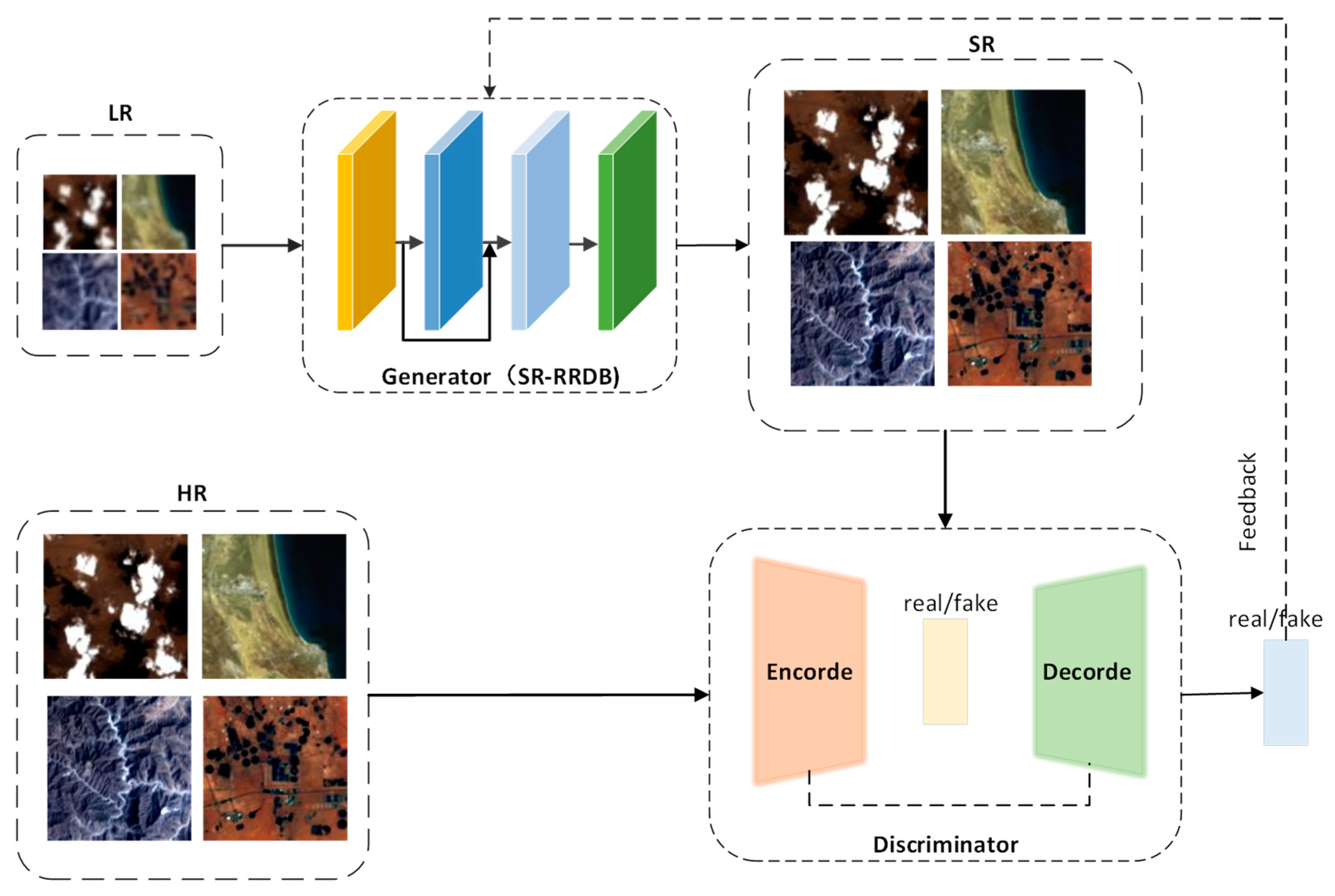
IESRGAN is composed of two main components: a generator and a discriminator. The overall workflow of IESRGAN is depicted in
Figure 1. The generator is responsible for taking an input LR remote sensing image and reconstructing an HR image. It achieves this by utilizing operations such as convolution and up-sampling within its network structure. The generator network learns to map the LR image to an SR image with enhanced details and finer textures. Once the SR image is generated, it is passed through the U-Net-based discriminator. The discriminator’s role is to compare the SR image with a real HR image and determine whether the SR image is realistic or not. The discriminator network is trained to identify flaws or discrepancies in the reconstructed images, enabling it to differentiate between real HR images and those generated by the generator. The generator and discriminator engage in continuous adversarial gameplay during training. The generator aims to produce SR images that are realistic enough to deceive the discriminator, while the discriminator strives to accurately identify the generated images. Through this adversarial process, both networks learn and improve their performance iteratively. As the training progresses, the generator becomes more adept at generating high-quality and realistic HR images. Simultaneously, the discriminator becomes more discerning and capable of detecting flaws in the reconstructed images. This iterative training process leads to the generation of HR images with enhanced details and improved realism.
2.1. Network Design of Generators—SR-RRDB
The generator network, depicted in
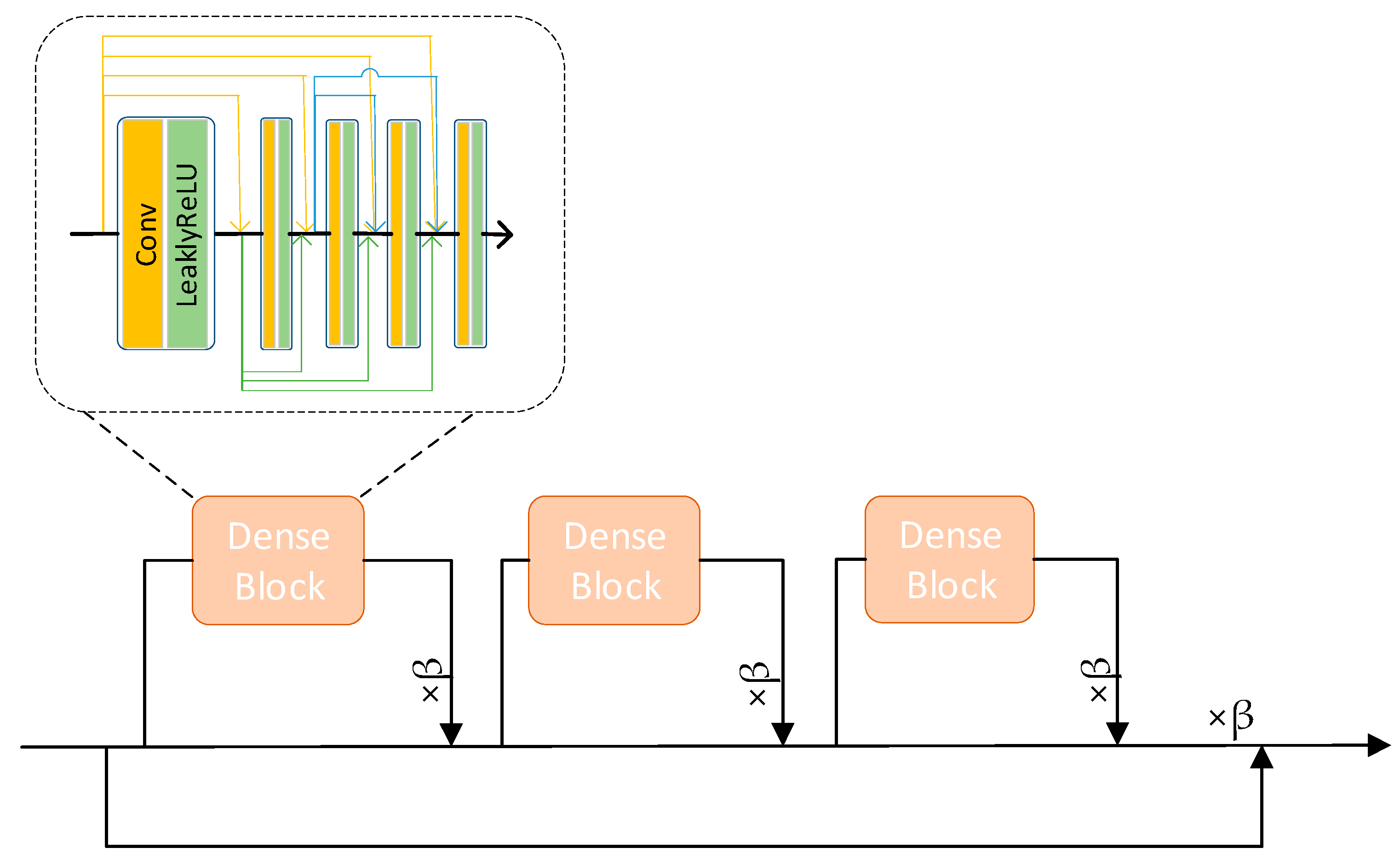
Figure 2, is a CNN-based model. Initially, the input image undergoes a reflection padding layer, referred to as the ReflectionPad layer, which prevents edge information loss. Following this, RRDB are utilized to retain detail features while uncovering new ones. Notably, the generator comprises four primary modules.
The first module is called the regular module, which consists of the ReflectionPad layer, Conv layer, and Rectified Linear Unit (ReLU) layer. The function of ReflectionPad is to perform reflection filling around the input image edges to extend edge information and avoid edge information loss and blurring; the Conv layer uses a 3 × 3 convolution kernel to perform convolution operation on the data in order to extract features; the ReLU layer performs a non-linear transformation to enhance the expressive power of the model. The ReLU layer has the advantages of simple computation, fast convergence, and no gradient disappearance problem.
The second module consists of 23 Residual-in-Residual Dense Block (RRDB) modules and a regular module with residual network connections. Among them, the RRDB combines the residual network structure and dense connectivity as shown in
Figure 3. The residual network learns the residuals between the input and output, and most of the residuals can be 0 or smaller [
34]. The dense connection is defined as
, where
denotes the network that combines
layer-generated feature map connections as input [
35]. Residual networks reuse features but are not good at mining new features while dense connections constantly explore new features but lead to higher redundancy [
36]. RRDB combines the advantages of both network structures to make the model better adapted to complex data distributions and patterns, improving performance and accuracy.
The third module is up-sampling, which is used to increase the image size.
The last module consists of two regular modules where the convolution kernel is changed from 1 × 1 to 3 × 3 to enlarge the perceptual field and to learn features better. With the above generator network structure, called SR-RRDB, a high-resolution image corresponding to the input image is reconstructed.
2.2. Discriminator Network Design
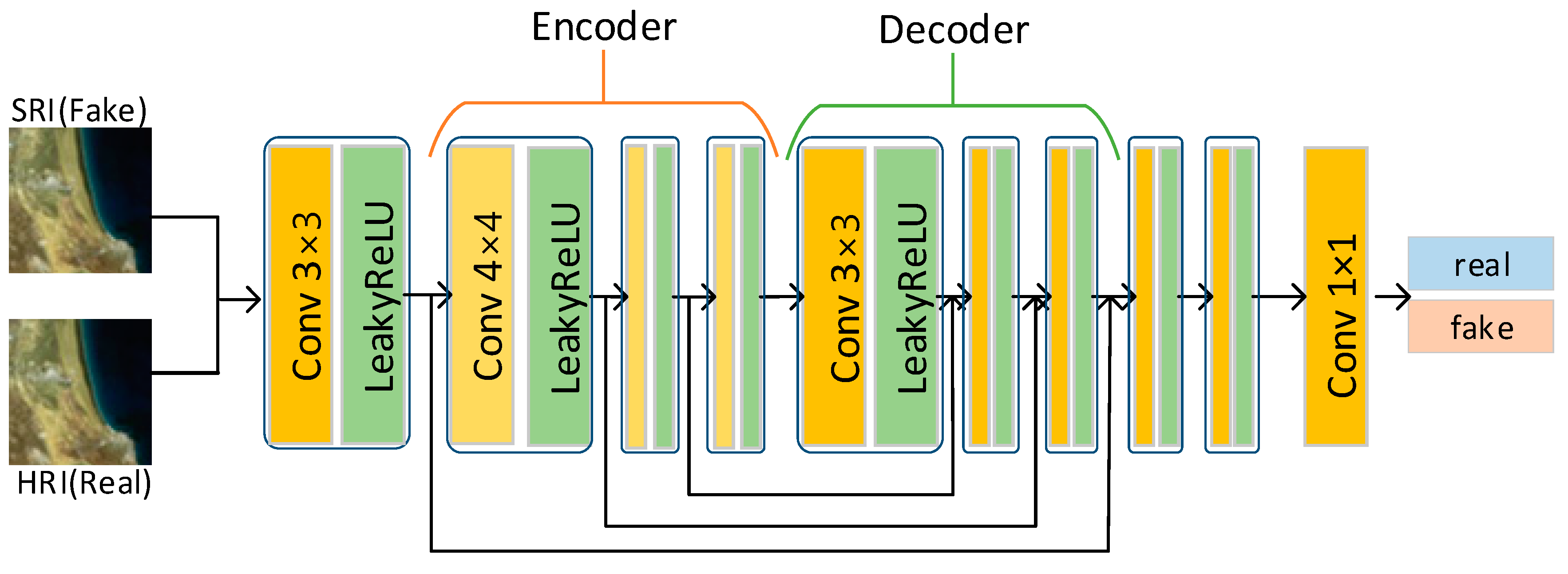
In this study, instead of using the traditional discriminator structure, we chose a discriminator network based on the U-Net structure, as shown in
Figure 4. This discriminator network structure consists of two main components: an encoder (down-sampling) and a decoder (up-sampling). The encoder is responsible for capturing the contextual information in the image, while the decoder is responsible for recovering the image details. To achieve information fusion, a jump connection is used between the two. As a result, this approach demonstrates its effectiveness in extracting multi-scale features from images with improved efficiency and accuracy.
It is worth noting that after entering the encoder from the initial convolution layer in this network structure, spectral normalization regularization is applied to stabilize the training of the discriminator network. Spectral normalization is a regularization method used in neural networks to prevent overfitting of neural networks by decomposing the weight matrix into eigenvalues and normalizing the result to limit the spectral norm of the weight matrix. The specific algorithmic process is presented in
Table 1. Spectral normalization [
37] makes the spectral norm of weight matrix
satisfy the Lipschitz constraint
= 1:
The use of a discriminator network based on the U-Net structure brings significant advantages. First, U-Net has jump connections, which fuse shallow features directly with deep features and alleviate the gradient disappearance problem. This allows the discriminator to learn semantic information at different scales and has a strong generalization capability. Secondly, since the U-Net structure fully considers the multi-scale information fusion, it can better capture the detail changes of small targets or local regions. This is important for generating high-quality images, especially in tasks that require the generation of fine structures and textures. Finally, U-Net restores features to the original input space step by step in the decoding stage by means of a deconvolution layer and continuously fuses shallow features. This allows the discriminator to take into account more contextual information, thus improving its ability to judge the quality of the generated images. Together, these advantages contribute to a significant improvement in GAN performance.
2.3. Loss Function
To enhance the robustness of the overall model, a fusion approach is employed in the loss function part. In the generator network, content loss, generation loss, and perceptual loss are included, where perceptual loss consists of content loss and generation loss. A binary cross entropy loss function (BCEWithLogitsLoss) is used in the discriminator network to counteract the loss.
The content loss is used to separately input the generated image and the target image into each convolutional layer in the VGG-19 network using the L1 norm and then calculate their differences in the feature space. The content loss formula is defined as:
Here,
represents the generated image,
denotes the target image,
signifies the feature map of layer
in the VGG-19 network, and
represents the L1 norm. The function of the content loss is to make the generated image closer to the pixel distribution of the target image, thus making the generated image more realistic. In the above formula, it is assumed that the feature map of a layer in the truncated VGG-19 network is represented as a three-dimensional tensor of
×
×
, where
indicates the number of channels,
indicates height, and
indicates width. Calculating generated image
at layer
feature map
, its definition is as follows:
where
denotes the feature value of generated image
at layer
, channel
, row
, and column
;
represents the value of the convolution kernel at position
in layer
, channel
, row
, and column
of the VGG-19 network.
indicates the feature value of generated image
at layer
, row
, and column
.
In the generation loss, the discriminator is used to discriminate whether the SR-generated image is a “pseudo-image” or not, and then the discriminant result is obtained. Then, the BCEWithLogitsLoss is used to calculate adversarial loss, which is the difference between the probability of the generated image being discriminated as a real image and 1. The BCEWithLogitsLoss formula is expressed as:
Here,
represents the number of samples,
denotes the label of the real image,
signifies the discriminant result of the discriminator on the generated image, and
stands for sigmoid function.
The overall perceptual loss is defined as written in Equation (9):
The discrimination loss is calculated using the BCEWithLogitsLoss. First, the discriminant results are obtained by discriminating the SR-generated images and the real images separately. Next, the SR-generated image tensor is assumed to be 0, which means “false image”, and the real image tensor is assumed to be 1, which means “true image”. The formula expression is:
where
and
are, respectively, represented as:
In this equation,
indicates the number of samples;
is assumed to be a tensor with all zeros, which denotes the label of the fake image;
is assumed to denote the discriminant result of the discriminator on the SR generated image, and
signifies a sigmoid function.
Here,
indicates the number of samples;
is assumed to be a tensor of all 1s, which denotes the label of the real image;
is assumed to denote the discriminant result of the real image, and
signifies a sigmoid function.
The BCEWithLogitsLoss is advantageous in calculating the generative loss and the adversarial loss because it can not only measure the difference between the prediction result and the true result but also convert the prediction result into a probability value through the sigmoid function transformation, thus, reflecting the confidence level of the prediction result more accurately. In addition, BCEWithLogitsLoss can automatically handle the numerical stability problem and prevent numerical overflow or underflow in the calculation of the sigmoid function. In the adversarial training process, using BCEWithLogitsLoss can effectively evaluate the similarity between the generated image and the real image and provide better guidance for generator training.
3. Experiments
In this paper, we conduct model experiments with the following data and compare classical models in the super-resolution domain to verify the validity and generalization of the model.
3.1. Data Source
The remote sensing image data selected for this study include NaSC-TG2 [
38], Satellite Images of Hurricane Damage [
39], NWPU-RESISC45 [
40], and UCMerced LandUse [
41]. The NaSC-TG2 data originate from China’s first space laboratory, Tiangong-2, which is equipped with a Wide-band Imaging Spectrometer (WIS) featuring 14 spectral channels covering visible light, near-infrared, short-wave infrared, and thermal infrared bands. The spatial resolution of these data at ground pixel distance is 100 m, 200 m, and 400 m. Satellite images of Hurricane Damage data are obtained from the Planet satellite constellation consisting of hundreds of Dove satellites (10 cm × 10 cm × 30 cm) that use optical systems and cameras to capture images in RGB and near-infrared bands with a ground pixel distance of 3~5 m. The NWPU-RESISC45 data come from Google Earth satellite images with spatial resolutions ranging from 0.2 m to 30 m, acquired through satellite imagery, aerial photography, and Geographic Information Systems (GIS). UCMerced LandUse data are sourced from the USGS National Map with a spatial resolution of 1 foot (0.3048 m).
Table 2 summarizes the information on SR remote sensing image data used in this paper. Considering the spectral range differences across channels in these satellite image datasets, our experimental data only include RGB three-band images. The selection of these datasets will aid in further exploring remote sensing image processing techniques and provide theoretical support for enhancing practical applications.
In our experiments, we built a training set using 19,980 remote sensing images from the NaSC-TG2 dataset. Each HR image was down-sampled by a factor of four to obtain a low-resolution LR image. The HR images have a size of 128 × 128 pixels, and correspondingly, the LR images have a size of 32 × 32 pixels. Training with smaller-sized images allows the model to focus on rich local textures, structural features, and object information in remote sensing images. This approach helps capture important details and patterns necessary for accurate super-resolution reconstruction. Additionally, using smaller-sized images reduces computational complexity and memory consumption.
Figure 5 illustrates examples of the HR–LR pairs. To evaluate the generalization capability of our proposed model, we constructed four test sets by randomly selecting 120 images from the NaSC-TG2 dataset, 1000 images from the Satellite Image of Hurricane Damage dataset, 1890 images from the NWPU-RESISC45 dataset, and 420 images from the UCMerced LandUse dataset. These diverse datasets provide a representative sample of remote sensing images, enabling us to assess how well our model performs on different types of scenes and objects. Through this comprehensive evaluation, we aim to demonstrate the robustness and effectiveness of our model in handling a variety of remotely sensed image scenes.
3.2. Experimental Environment and Parameter Settings
In this study, the experimental environment was set up on an Ubuntu operating system, equipped with a high-performance GeForce RTX 2080Ti GPU for efficient computation. The programming language utilized for code development is Python, while the Pytorch framework (available at
https://pytorch.org/ (accessed on 1 July 2023)) was employed for effective algorithm modeling and implementation. The IESRGAN network architecture comprises two primary components: the generator network and the discriminator network. To conduct the experiments, a total of 19,800 HR remote sensing images from the NaSC-TG2 dataset were employed as the target images. As an initial step, a bicubic interpolation down-sampling technique was applied to generate a corresponding set of 19,800 LR remote sensing images required for input purposes. Subsequently, these LR images were fed into the SR-RRDB model, which consists of the generator network designed for training purposes. A comprehensive overview of the initial experimental details pertaining to the SR-RRDB model training can be found in
Table 3.
The Cosine Annealing Learning Rate Schedule (CosineAnnealingLR) scheduler combined with the Adam optimizer was employed to effectively adjust learning rates during the training process. This method allows for the gradual reduction of learning rates, which in turn leads to enhanced convergence and ultimately improves the overall performance and generalization capability of the model. Upon completing this stage, the SR images generated by the well-trained SR-RRDB model were then introduced into a discriminator network that was designed based on the U-Net architecture. The purpose of this step was to efficiently discriminate between real HR images and those produced by the SR-RRDB model. Starting with the initialization of the SR-RRDB model, further experimental details pertaining to IESRGAN model training can be observed in
Table 4. Notably, when the training reached its halfway point, there was an adjustment made wherein the learning rate was deliberately reduced to a half of its initial value. This strategic modification has been found to contribute significantly towards optimizing and refining both model performance and generalization effectiveness throughout the training process.
Figure 6 below shows the change curves of content loss, generation loss, and discriminative loss, respectively, throughout the training process.
3.3. Experimental Evaluation Metrics
The Peak Signal-to-Noise Ratio (PSNR) [
42] and Structural Similarity Index (SSIM) [
43] have been used as standard evaluation metrics in image SR. Nevertheless, as revealed in some recent studies [
44], super-resolved images may sometimes have high PSNR and SSIM scores with over-smoothed results but tend to lack realistic visual results. In this study, apart from the PSNR and SSIM, the learned perceptual image patch similarity (LPIPS) [
45] is included in our experiments.
PSNR is used to evaluate pixel-wise differences between images. A higher PSNR value indicates a smaller difference between the processed image and the real image, implying better image quality. Its formula is:
In this formula,
MAX represents the maximum pixel value, and
MSE denotes the mean squared error between the reference image and the evaluated image. Its formula is given by:
Here, N refers to the total number of pixels, while and represent the th pixel values of the reference image and evaluated image, respectively.
SSIM takes into account factors such as the brightness, contrast, and structure of an image. Its formula is expressed as:
The SSIM value ranges from [0,1] with higher values indicating better image quality.
LPIPS measures perceptual differences between two images, i.e., visual similarity between generated images and real images. A lower LPIPS score indicates a higher similarity between two images. Its formula is as follows:
In the above equation, and represent generated images and real images, respectively; denotes predicted feature maps for x at spatial position and feature map ; represents predicted feature maps for at the same spatial position and feature map. The weight matrix is learned by the network to emphasize or de-emphasize certain features in an image.
3.4. Quantitative and Qualitative Comparison of Different Methods
In this section, an in-depth comparison is conducted between the proposed method and several classical single-image SR algorithms on four distinct test sets, focusing on their performance metrics. The SR algorithms under consideration encompass three CNN-based methods, specifically VDSR [
17], SRResNet [
22], and TESR [
30], as well as two GAN-based methods, namely SRGAN [
22] and ESRGAN [
23]. Each of these methods has been meticulously optimized on the training set to guarantee the best possible performance and to ensure a fair comparison. To facilitate a more comprehensive comparison with both CNN-based and GAN-based algorithms, two networks are trained: SR-RRDB and IESRGAN. The proposed SR-RRDB is primarily a CNN-based algorithm that consists solely of the generator network. When trained exclusively with pixel loss, it can independently reconstruct HR images corresponding to LR ones. However, this approach may lack human perception since it relies solely on pixel loss for optimization. Therefore, a fair comparison between SR-RRDB and other CNN-based algorithms is made to evaluate their performance. On the other hand, the proposed IESRGAN is constructed upon a GAN network model, comprising both generator and discriminator networks. Its loss function incorporates perceptual loss through an innovative fusion method, which significantly enhances visual quality as perceived by the human eye. Thus, a fair comparison between IESRGAN and other GAN-based algorithms is conducted to assess their ability in delivering visually appealing results. In summary, this section aims to provide an extensive evaluation of the proposed method against traditional single-image SR algorithms in terms of performance metrics across four test sets. By comparing both CNN-based and GAN-based approaches using two different networks (SR-RRDB and IESRGAN), we strive to present a balanced analysis that highlights the strengths and limitations of each method while ensuring fairness in comparisons.
In this study, three metrics are employed to quantitatively evaluate the SR results, namely PSNR, SSIM, and LPIPS. The best results in each row are highlighted in red for easy comparison. As demonstrated in
Table 5, the highest score in the PSNR metric is achieved by the SR-RRDB method. Here it is noted that a higher PSNR value indicates a lower difference between the reconstructed image and the real image, ultimately resulting in superior image quality. As shown in
Table 6, the highest score on the SSIM metric is also attained by the SR-RRDB method. A higher SSIM value suggests a greater similarity in brightness, contrast, and structure within a range of [0,1], indicating better preservation of these attributes during the super resolution process. Meanwhile, as displayed in
Table 7, IESRGAN performs best on the LPIPS metric; a lower LPIPS value implies higher visual perceptual similarity between generated and real images. CNN-based SR methods offer advantages in terms of PSNR and SSIM due to their emphasis on preserving LR images’ spatial structure. Consequently, super-resolution outcomes from CNN-based methods tend to lack realistic visual effects, leading to poor LPIPS performance. In contrast, GAN-based SR methods achieve better LPIPS performance while maintaining good PSNR and SSIM scores as they adopt adversarial loss and perceptual loss to encourage visually appealing results that closely resemble real images.
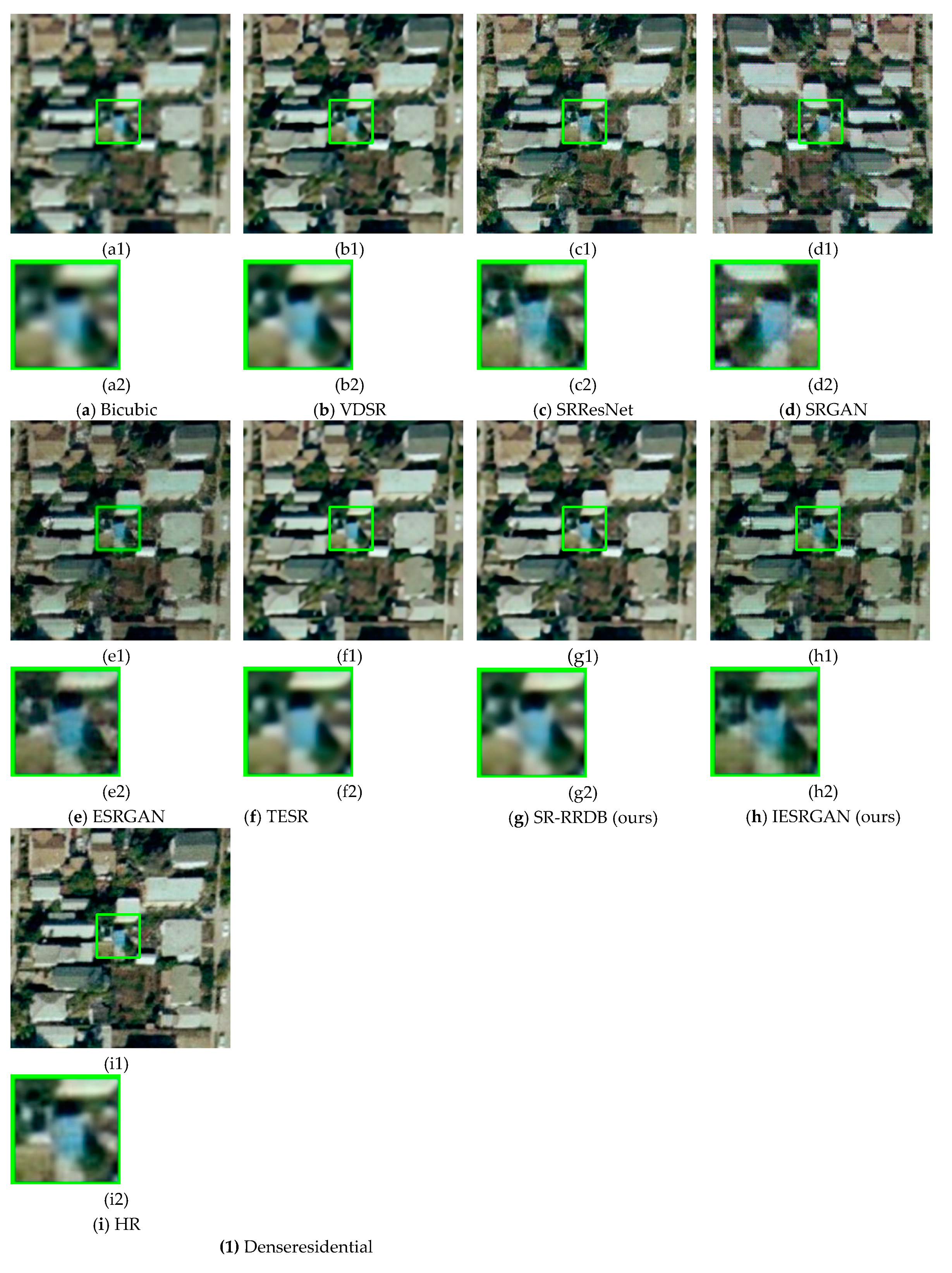
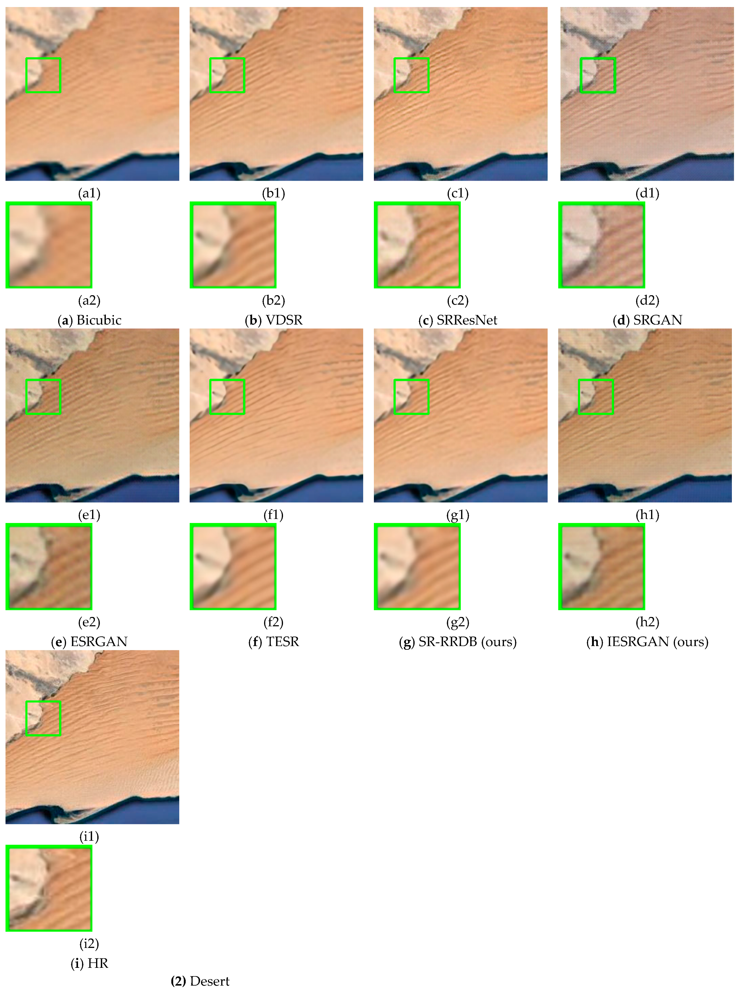
Figure 7 presents a comprehensive and intuitive comparison that enables a more profound comprehension of the quantitative results obtained in this study. Bicubic interpolation, as a traditional method, fails to generate any additional details or enhance image quality significantly. On the other hand, CNN-based super-resolution reconstruction algorithms, such as VDSR, SRResNet, and TESR, demonstrate relatively better performance in reconstructing some texture details by leveraging advanced learning techniques; however, they still suffer from contour blurring issues primarily due to the adoption of simplistic optimization strategies in their objective functions. In contrast, GAN-based super-resolution reconstruction algorithms like SRGAN and ESRGAN showcase notable advantages in terms of visual effects and overall image enhancement. Nevertheless, these methods may inadvertently introduce artificial artifacts during the reconstruction process, which could potentially compromise the final output quality. The approach proposed here addresses these limitations by effectively recovering finer texture details compared to other SR methods available in the literature. Consequently, our method generates more realistic and visually appealing results that closely resemble natural images. This superior performance can be attributed to the innovative techniques employed in our algorithm design, which strike a delicate balance between optimizing visual quality and minimizing unwanted artifacts.
3.5. Ablation Studies
In order to assess the effectiveness of the enhancements introduced by each component of our proposed method, a series of ablation experiments was performed. In these experiments, we gradually incorporated the RRDB strategy, Reflection Padding layer (ReflectionPad), and U-Net structure into the baseline model. All models were trained using an identical configuration, and their performance was evaluated on a test set. The comparative data for various metrics are presented in
Table 8, which clearly demonstrates an overall improvement in model performance throughout the refinement process.
Initially, increasing the number of RRDBs effectively contributes to enhancing image details and high-frequency information. This enhancement is achieved by mapping the image from an LR to an HR space through a deep network structure. Consequently, more image details are recovered, resulting in notable improvements in PSNR, SSIM, and LPIPS scores. Subsequently, adding a Reflection Padding layer on top of this foundation helps preserve edge information within the input image while reducing edge information loss. Edge information plays a critical role in generating HR images since it often contains high-frequency detail information that influences the level of detail present in the generated results. By introducing the Reflection Padding layer into our model, we achieve optimal SSIM values indicative of relatively ideal structural reconstruction effects. Lastly, incorporating a U-Net structure into the discriminator enables it to capture and integrate image features across multiple resolution levels more effectively. This enhanced capability assists in distinguishing generated images from real ones while simultaneously improving reconstructed image quality. In conjunction with our adopted fusion loss approach, this results in superior LPIPS values and improved perceptual quality for human observers. At the same time, both the PSNR and SSIM scores exhibit some degree of improvement as well—evidence that our model delivers higher-quality images. In summary, following these step-by-step enhancements to our initial design, our proposed method achieves significant improvements across all relevant metrics—thereby validating the effectiveness of each modification introduced.
