Article

Ground-Based Remote Sensing of Atmospheric Water Vapor Using High-Resolution FTIR Spectrometry

1
University of Science and Technology of China, Hefei 230026, China
2
Key Laboratory of Environmental Optics and Technology, Anhui Institute of Optics and Fine Mechanics, Chinese Academy of Sciences, Hefei 230031, China
3
Guangdong-Hongkong-Macau Joint Laboratory of Collaborative Innovation for Environmental Quality, Guangzhou 510000, China
4
Key Laboratory of Middle Atmosphere and Global Environment Observation, Beijing 100084, China
5
State Environmental Protection Key Laboratory of Sources and Control of Air Pollution Complex, Beijing 100084, China
6
Center for Excellence in Regional Atmospheric Environment, Institute of Urban Environment, Chinese Academy of Sciences, Xiamen 361021, China
7
Department of Automation, Hefei University, Hefei 230601, China
*
Author to whom correspondence should be addressed.
Remote Sens. 2023, 15(14), 3484; https://doi.org/10.3390/rs15143484
Submission received: 26 May 2023 / Revised: 1 July 2023 / Accepted: 7 July 2023 / Published: 11 July 2023
(This article belongs to the Special Issue Remote Sensing of Atmospheric Composition)

Abstract

:
Understanding the distribution of atmospheric water vapor (H2O) is crucial for global warming studies and climate change mitigation. In this study, we retrieved the ground layer, tropospheric and total columns of H2O using ground-based high-resolution Fourier transform infrared spectrometry (FTIR). The H2O total columns are obtained from near-infrared (NIR) and mid-infrared (MIR) spectra, and the ground layer and tropospheric H2O columns are retrieved from the MIR spectrum. The total columns of H2O retrieved from NIR and MIR have a good consistency (R = 0.989). Additionally, the ground layer H2O columns have a similar seasonal variation to total columns and tropospheric columns but have a higher seasonal amplitude. The ground layer H2O columns are close to the total columns and tropospheric columns in winter; however, in summer, the average difference between the ground layer and total columns and the value between the ground layer and tropospheric columns are large. This is mostly due to temperature variation. The temperature has a linear response to H2O, and the relationship between surface temperature and ln(XH2O) values in the ground layer, the entire atmosphere and the troposphere show a significantly positive correlation, and the correlation coefficient R is 0.893, 0.882 and 0.683, respectively. Furthermore, we selected the HYSPLIT model to simulate the back trajectories of air parcels in the four seasons in Hefei and find that the air mass transport has a significant impact on the local H2O change. These results demonstrate that ground-based high-resolution FTIR technology has high accuracy and precision in observing the vertical distribution and seasonal changes of H2O in different atmospheres.

1. Introduction

Water vapor (H2O) in the atmosphere is the most abundant greenhouse gas (GHG) and plays a significant role in atmospheric chemistry and climate change [1]. The most important meteorology is that the characteristics of weather change are closely related to regional transport and seasonal variation of H2O in the atmosphere. Without H2O, there would be no clouds, rain and snow as these substances cannot exist without H2O [2]. Moreover, H2O is also the most important GHG on earth that people depend on for survival; about 90% of the global natural greenhouse effect comes from H2O, and keeps the earth warm enough to support life [3,4]. An increase in H2O will lead to an increase in temperature, which will cause more H2O to be absorbed into the air. Climate warming and water absorption will increase in a spiral cycle [5,6,7]. The observed climate warming leads to an increase in comprehensive H2O, which in turn forces further climate change [8,9]. Therefore, assessing and quantifying atmospheric H2O is critical to constraining weather and climate models.
H2O mostly exists in the troposphere, only 10% of which is up to 850 hPa and 40% up to 500 hPa [10]. H2O has been measured by many methods and techniques. Spaceborne infrared instruments have the advantage of large-scale measurements but lack long-term and vertical data [11]. In addition, H2O measured by satellite is often accompanied by large uncertainty, which must be verified before analysis [12]. The in situ sensors have very high accuracy and precision, but the measurement of H2O concentration near the ground is easily affected by the landform and the vertical transmission of air masses [13,14]. Remote sensing measurement techniques can avoid the interference of the above factors. High-precision and high-accuracy remote sensing can provide key information on H2O column concentration [15,16,17].
The ground-based high-resolution Fourier transform infrared spectrometer (FTIR) records the direct sunlight to observe the H2O, which has high precision and accuracy. Moreover, the ground-based FTIR measurement has long-term stability, so it can be used to verify the satellite H2O information and model simulations. The total carbon column observing network (TCCON) and the network for the detection of atmospheric composition change (NDACC) use high-resolution FTIR instruments to record solar absorption spectra in the near-infrared (NIR) and mid-infrared (MIR) band, respectively, so as to obtain the total column-averaged dry-air mole fraction (DMF) of H2O [18]. Recently, many projects have been conducted in different geographical regions to compare different methods of H2O observation. Makarova et al. (2014) made intercomparison techniques of satellite, airborne and FTIR at Tomsk for observations of H2O [19]. Yana et al. (2017) compared the simultaneous datasets of H2O measured by the NDACC measurement, RPG-HATPRO microwave radiometer and Novatel ProPak-V3 global navigation satellite system receiver at the St. Petersburg site [20]. Tu et al. (2020) compared column-averaged dry-air mole fractions of H2O from the collaborative carbon column observing network (COCCON) with retrievals from the TCCON measurements and the NDACC measurements as references at two northern observation sites [21]. Therefore, long-term records of H2O can be provided, including time and a certain degree of spatial coverage. However, there are also some challenges in retrieving H2O based on ground-based FTIR spectroscopy, such as the instability of the retrieved vertical profile, the large error of the retrieval result and the low degrees of freedom for signal (DOFs) of the retrieval result [22,23].
In this study, we focused on the FTIR technique for H2O retrieval and on the data from the Bruker 125 HR spectrometer. We analyzed the FTIR retrievals of NIR and MIR, provide their spectral and column average kernels, and compared the column-averaged dry-air mole fractions of H2O (XH2O) in the two spectral regions with the aim of understanding the H2O vertical distribution in the atmosphere. Focused on the measurement of H2O in MIR, we calculated its error budget and divided the atmosphere into two independent layers based on the calculated DMF. Afterward, we gave the characteristics of H2O variation in the atmosphere, inferred the relationship between H2O and surface temperature, and analyzed the main sources of H2O.
Section 2 gives an introduction to the Hefei site and the measurement instrument and describes the H2O retrieval method and the error budget. The H2O total columns, ground layer H2O columns and tropospheric H2O columns are compared in Section 3, and the seasonal variation of H2O is discussed. Moreover, the main sources of H2O based on the back trajectories of air masses are clarified in this Section. The conclusions are made in Section 4.

2. Instrument and Retrieval Strategy

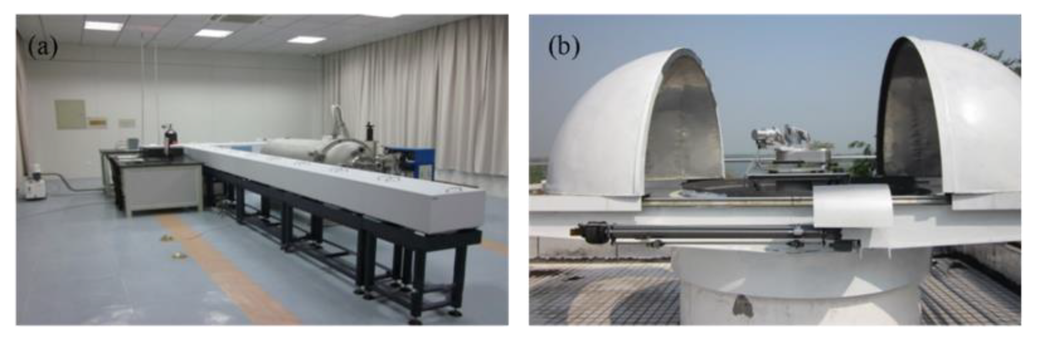
2.1. Instrument and Site Description

The observation site (31.540°N, 117.100°E, 29 m) is located in the northwest suburb of Hefei City, Anhui Province, China. The site installed a ground-based remote sensing system in January 2014, consisting of a high-resolution FTIR spectrometer (Bruker IFS 125HR, Waltham, MA, USA) and a solar tracker (A547N) produced by Bruker optics, Germany (Figure 1). The solar tracker is mounted on the roof of the laboratory and protected by a protective cover, with tracking accuracy of 0.1°. A meteorological station (ZENO, Coastal Environmental Systems, Dallas, TX, USA), on the roof of the laboratory that is near the solar tracker, has recorded information including surface temperature, surface pressure, wind speed, wind direction, humidity, rain and snow and leaf wetness data since September 2015 [22,23,24].
As shown in Table 1, we use the FTIR instrument to collect NIR spectra (4000–11,000 cm−1) and MIR spectra (600–4500 cm−1) during clear days. To maximize the signal-to-noise ratio (SNR) of the MIR spectra, the spectra are recorded using optical band-pass filters. FTIR infrared spectra have a continuum SNR of more than 80 over much of the spectral range. The NIR spectra are recorded by the FTIR instrument equipped with the calcium fluoride (CaF2) beam splitter and indium gallium arsenide (InGaAs) detector, and a nominal spectral resolution of 0.02 cm−1 (optical path difference of 45 cm) [22,23]. The MIR spectra with a spectral resolution up to 0.005 cm−1 (optical path difference of 180 cm) are recorded by liquid-nitrogen-cooled indium antimonide (InSb) and mercury cadmium telluride (MCT) detectors along with a potassium bromide (KBr) beam splitter [22,24]. To ensure the stability of the measurement, the instrument is vacuumized under 50 hPa. The instrument line shape (ILS) is required to diagnose the collimation state of the optical path of the spectrometer, so that the total columns and profile of gases from measurements are retrieved precisely [22,25,26]. The ILS is monitored by low-pressure HCl and HBr cell measurements for near-infrared and mid-infrared range, respectively [22,27,28].

2.2. The Retrieval Strategy of NIR H2O Column

The GGG2020 software package uses a nonlinear least square spectral fitting algorithm (GFIT) to retrieve the H2O total column [29]. The daily temperature and pressure profiles are also obtained from the NCEP data. Spectroscopic line parameters are adopted from the HITRAN 2012 database [30,31]. A set of spectral micro-windows for H2O are chosen to retrieve the concentration by considering the minimum absorption of other interfering species (CH4, CO and CO2). GGG2020 calculates the total column of H2O, and then the column-averaged DMF of the H2O is computed as:
X H 2 O = c o l u m n H 2 O c o l u m n a i r d r y = 0.2095 × c o l u m n H 2 O c o l u m n O 2
where c o l u m n H 2 O is the column concentration of H2O and c o l u m n O 2 is the column concentration of oxygen in the atmosphere. The column of dry air, in molecules/cm2, is calculated from the oxygen (O2) column divided by 0.2095 [32]. The advantage of dividing by O2 column abundance is that it reduces the systematic uncertainties from the parameters that affect the retrievals of both species similarly, e.g., such as instrument line shape (ILS) and the solar zenith angle (SZA). Figure 2 depicts a typical spectral fitting (observed at 04:44 UTC 3 February 2016, with an SZA of 48.82°) of H2O in the spectral windows listed in Table 2. The root-mean-square error of spectral fitting residuals is 0.16% for H2O. The average signal–to–noise ratio is 87.6.
Figure 3 gives the total column averaging kernels of H2O observed at different SZAs. The range of SZAs for NIR spectra is mainly from 20 to 70° at the Hefei site. The sensitivity of height dependence of the retrieved profile to concentration perturbations at different atmospheric levels is represented by the total column averaging kernel [22]. The ideal total column averaging kernels should be 1.0 at each altitude, meaning that the retrieved results are the same as the true states. However, the actual total column averaging kernel of H2O is not equal to 1.0. If the value is greater than 1.0 for a height, it means that the retrieved results overestimate the contribution of that particular layer to the total column budget, and vice versa [33]. As a result, the near-infrared retrieved H2O total column underestimates the a priori in the lower troposphere and overestimates it at high altitudes.

2.3. The Retrieval Strategy of MIR H2O Column

In contrast to the above method, the MIR H2O column is retrieved by the SFIT4 (version 0.9.4.4) based on the optimal estimation method [34]. MIR spectra containing strong and well-isolated H2O absorption lines are selected as micro-windows for H2O retrieval [13,35,36]. Additionally, the spectral signatures of interfering gases (CH4, N2O, O3 and HCl) are also considered to reduce fitting residuals. Table 3 shows the retrieval parameters and interfering gases for H2O at the Hefei site. Four retrieval windows of H2O were fitted at the same time. The NCEP reanalysis data were used for the a priori profiles of atmospheric temperature, pressure and H2O [37]. The spectroscopic line parameters for H2O and interfering species are derived from the HITRAN 2012 line list [38]. For MIR retrieval, the X H 2 O results are different to NIR results, because it is difficult to retrieve O 2 total column from MIR spectra. The X H 2 O column is calculated as:
X H 2 O = c o l u m n H 2 O c o l u m n d r y   a i r = c o l u m n H 2 O p s g m a i r d r y c o l u m n H 2 O m H 2 O m a i r d r y
where p s is the surface pressure; g is the column–averaged gravitational acceleration; m H 2 O and m a i r d r y are the molecular masses of H2O and dry air, respectively; and c o l u m n H 2 O is the total column of H2O observed from NCEP reanalysis data. The ground surface pressures are recorded by the meteorological station, with an accuracy better than 0.1 hPa. A typical H2O absorbed spectrum was collected at 03:25 UTC 31 December 2020, with a SZA of 56.22° (Figure 4). The root–mean–square errors are 0.267%, 0.372%, 0.452% and 0.205%, respectively, showing that the spectrum is well–fitted.
Figure 5 presents the measured H2O profiles and the a priori profile during the observation period from 2016 to 2020 at the Hefei site. As shown in Figure 5, the concentrations of H2O are small and very close to the a priori profile above the tropopause, with concentrations in the ground layer that are higher than those in the troposphere. H2O mostly exists in the ground layer. The averaging kernels matrix is used to depict the sensitivity of height dependence of the retrieved profile to concentration perturbations at the various atmospheric levels [22,39]. The typical averaging kernel matrix of H2O is shown in Figure 6. The most sensitive height range for H2O is mainly located below 10km. H2O retrievals have a good sensitivity to the whole troposphere and lower stratosphere. The trace of averaging kernel matrix is characterized as DOFs [22]. As is shown in Figure 7, the typical DOFs for H2O over Hefei are about 2.53. This indicates that the retrieved profile can be separated into two independent partial columns, because the criterion for separating columns into separate layers is that the column DOFs of gases is greater than 1.0 [22,40,41]. We calculate the ground layer H2O DMF from 0 to 2.95 km with the DOFs of 1.06, and the tropospheric H2O DMF from 2.95 to 15 km.

2.4. Error Analysis of MIR H2O Retrieval

The retrieval errors of MIR results contain random and systematic sources, and the error analysis is performed using a posterior error estimation method based on Rodgers, which calculates errors by attributing them to each parameter used in the retrieval [39]. The retrieved H2O column is in fact an estimate of a state smoothed by the averaging kernel. The smoothing error ( S s ) is the difference between these two states.
S s = A I S a A I T
S a   is a prior covariance matrix, I represents a unit matrix and A is the averaging kernel. The retrieval parameter error is the errors in the retrieval parameters, such as temperature profile, SZA, spectroscopic line parameters and field of view [42]. This error covariance matrix is calculated as:
S b = G y K b S b G y K b T
S b is the error covariance, G y is the sensitivity of measurement results to measurement and K b is the matrix of the weighting function of the parameters of the forward model. As shown in Table 4, for the temperature distribution used in a priori, we set the uncertainty as 3K. The systematic uncertainty values of the line intensity, line T broadening and line P broadening solar line are selected as 1%, 10% and 3% [22]. By analyzing the saturated absorption line, we concluded that the solar zenith angle, solar line shift and solar line strength uncertainty are selected as 0.025°, 0.005 cm 1 and 0.1%. We also considered the field of view uncertainty about 0.001. In addition, we used uncertainty values of 2% for the spectroscopic parameters of H2O [15].
The results of the error analysis for a typical H2O retrieval (03:25 UTC 31 December 2020, with a solar zenith angle of 56.22°) are summarized in Table 5. The total random and systematic errors for H2O column are about 6.49% and 1.55%, respectively. The very low retrieval error has already been proven in previous studies [43,44]. It is clear that the temperature profile uncertainties are the main random error and system error sources, accounting for 6.43% and 1.08%, respectively. The errors due to uncertainties of smoothing error and measurement error are very small, accounting for 0.026% and 0.05%. The systematic error of H2O is mainly determined by the uncertainty of the temperature profile.

3. Results and Discussion

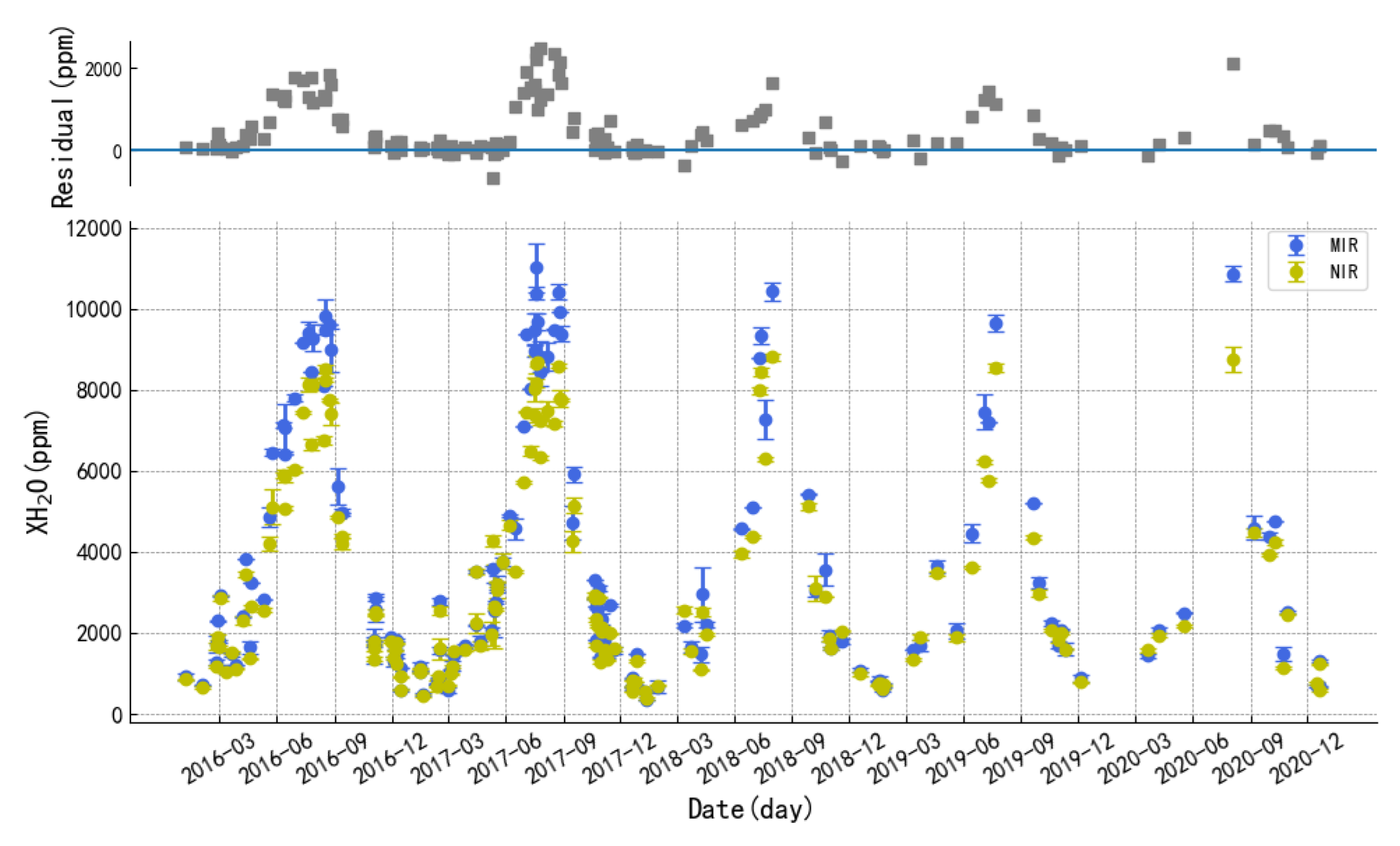
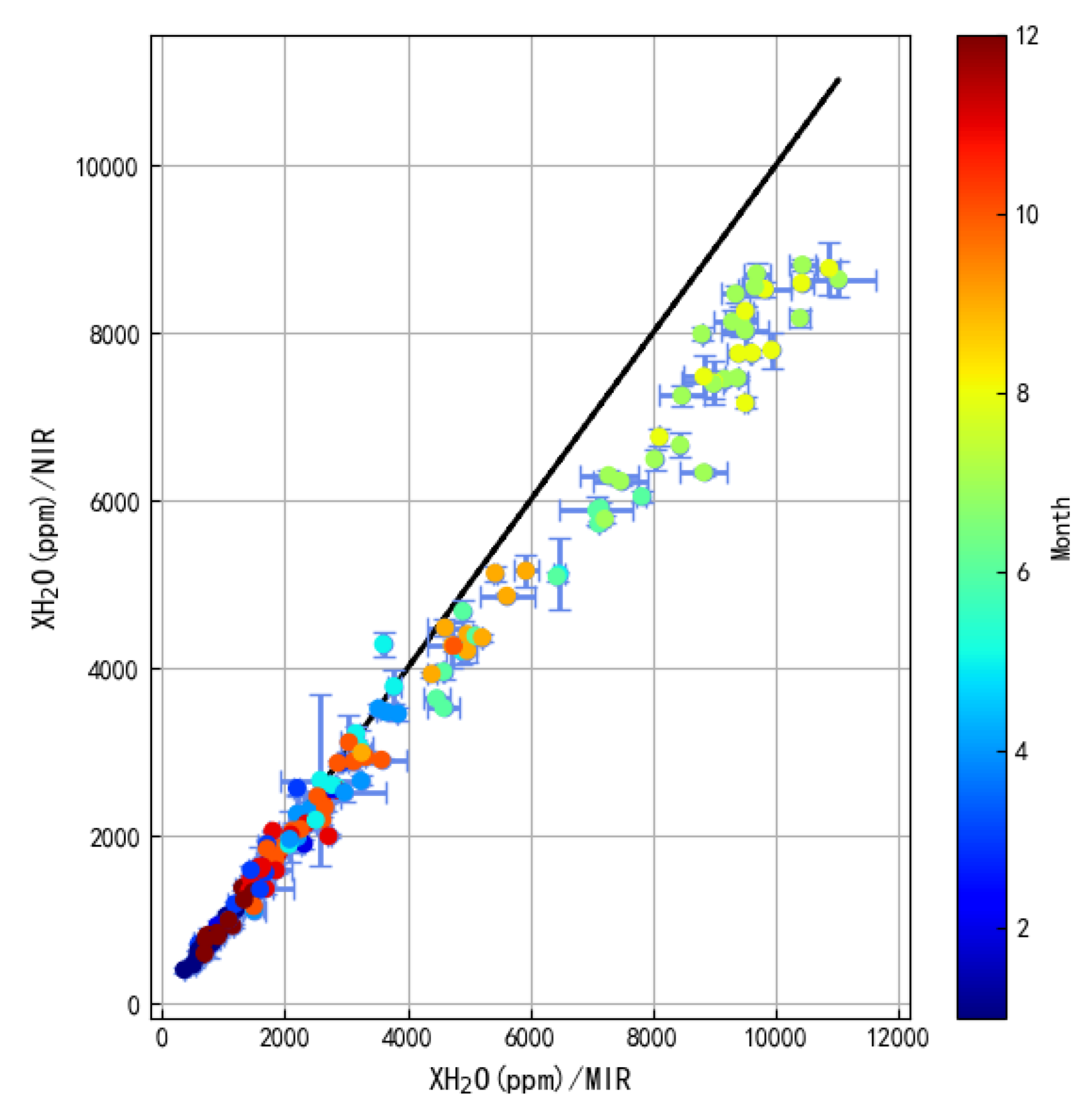
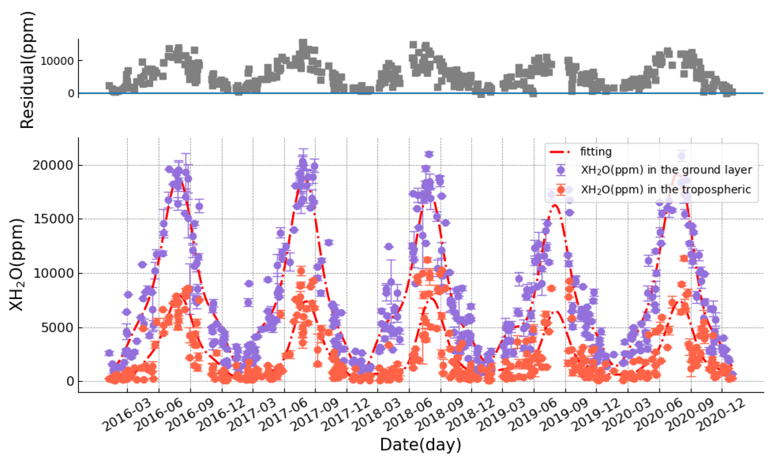
3.1. Time Series of XH2O

The DMF of H2O retrieved from near-infrared spectra was compared with the values retrieved from mid-infrared spectra. For NIR-spectra-derived products, O2 total columns are simultaneously retrieved with the target species. The NIR-spectra-derived XH2O are calculated based on Equation (1). For MIR-spectra-derived products, there are no N2 or O2 absorption windows that allow sufficient accuracy for column abundance retrieval. Therefore, the MIR-spectra-derived DMF of H2O are calculated based on Equation (2). For quantitative comparisons, we used the co-located daily means of FTIR measurements at the site. It should be noted that the FTIR instrument collects direct solar radiation, and the measurements depend on clear skies.
The time series of near-infrared and mid-infrared spectra-derived XH2O data from January 2016 to December 2020 are depicted in Figure 8. Some data are missing from the ground-based FTIR data due to high SZA conditions and poor weather. The variation trend of XH2O obtained from near-infrared spectra is similar to that obtained from mid-infrared spectra, both showing obvious seasonal changes over the observation period. There are higher amounts of atmospheric XH2O in summer than in other seasons, and the seasonal changes in the five years are consistent. For NIR-spectra-derived results, XH2O peaked each August, and the daily averaged XH2O reached the peak with the range of 7439.34~8443.83 ppm, while there is only 525.17~907.52 ppm for the minimum XH2O in each early spring and winter. XH2O amounts from mid-infrared spectra are slightly higher than the corresponding values from near-infrared spectra, especially in summer. XH2O from mid-infrared spectra reach up to 7894.22~9665.07 ppm each August 2016 to 2019; meanwhile, it reduced to 526.15~875.60 ppm for the minimum in each early spring and winter. This corresponds to the seasonal variation in temperature, which is the major reason for H2O variation in the atmosphere [21]. The mean bias, defined as the average difference in XH2O between simultaneous MIR and NIR data, is approximately 480.52 ppm. The difference is due to using different calculation methods. In addition, the SZA differences also cause the difference of XH2O from mid-infrared and near-infrared spectra, because both retrievals are dependent on solar zenith angles [45].
As shown in Figure 9, the time series of MIR spectra derived XH2O are compared with the NIR spectra derived data observed from January 2016 to December 2020. To co-locate the MIR data with the NIR data, the daily averaged data observed on the same day were directly compared, and the datasets that have at least four individual measurements within one day are used for the data average. To eliminate the effect of different a priori profiles and averaging kernels on XH2O, we used the a priori profile of the MIR retrievals to correct the NIR retrieved data [46]. There is a high correlation between MIR and NIR data (R = 0.989). It is concluded that MIR-spectra-derived XH2O agrees well with the NIR observations. These time series show that MIR and NIR spectra measurements are able to capture the seasonal variations of atmospheric H2O. However, MIR and NIR data show a higher correlation coefficient in the winter period than that in the summer, and the slope ratio is closer to one in the winter. This is mainly due to the MIR observations having higher H2O values than the NIR results in summer.

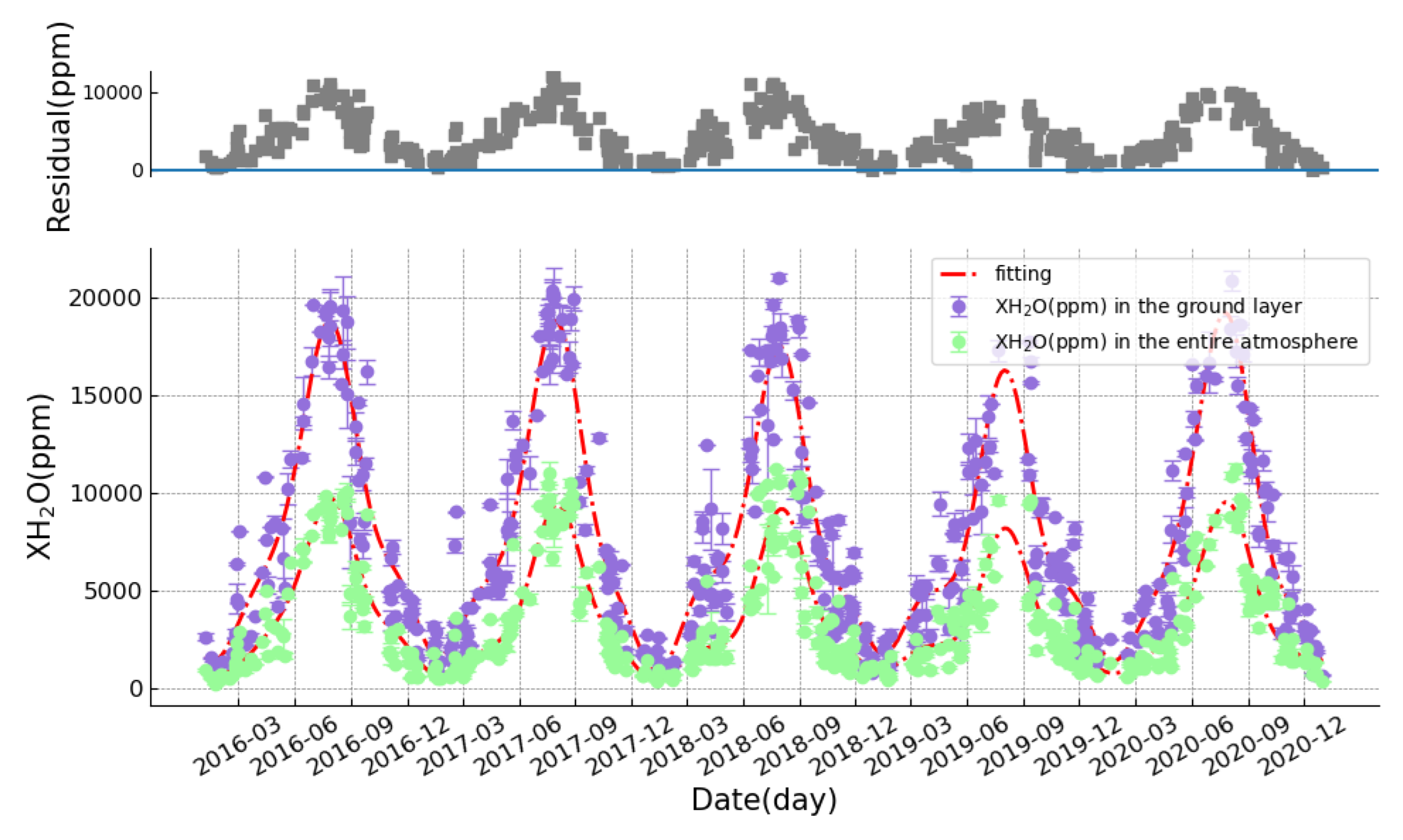
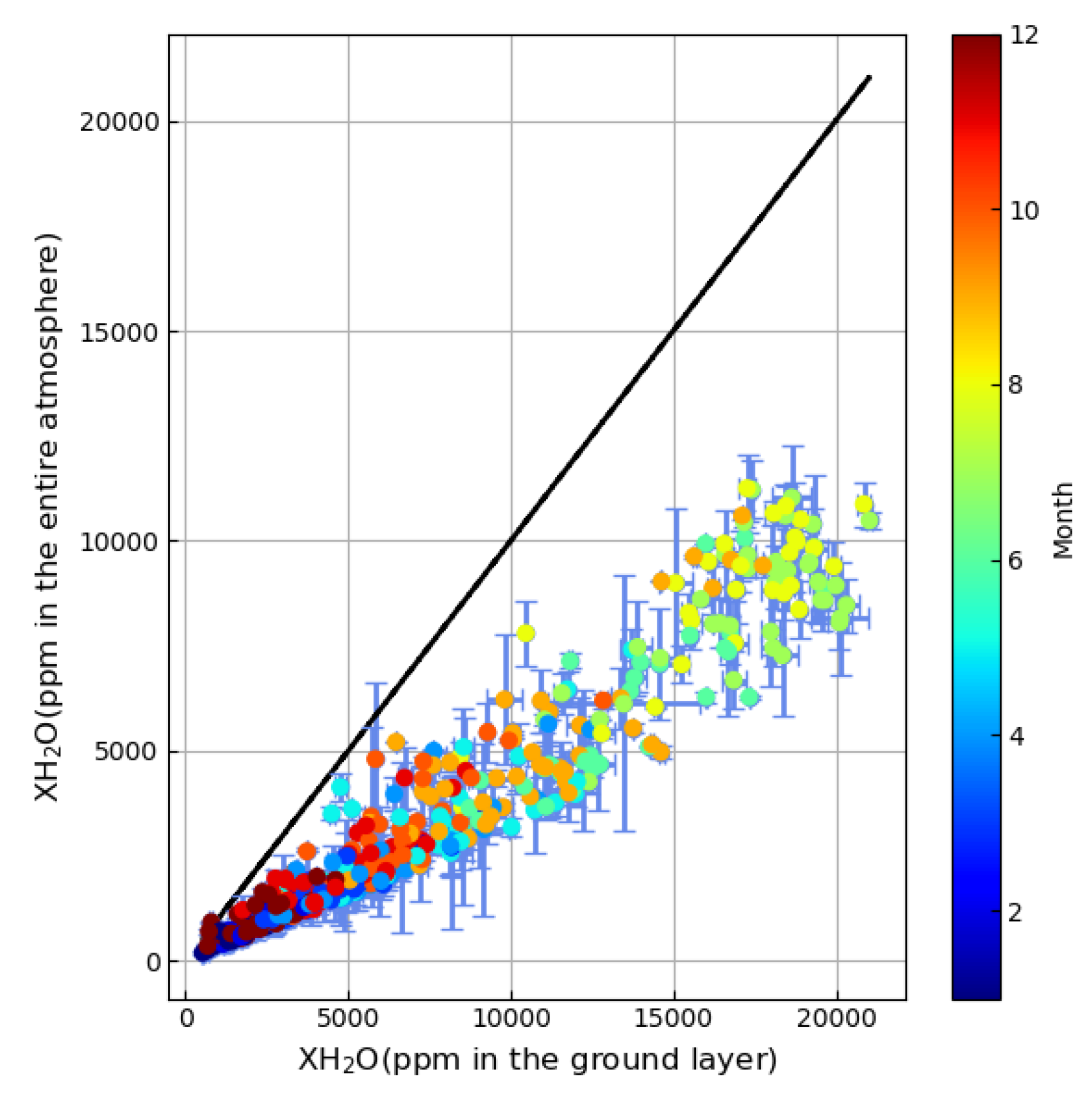
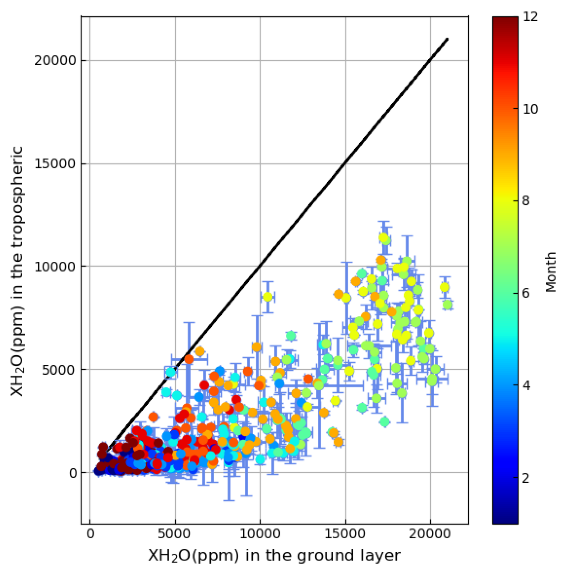
3.2. Time Series of H2O in the Ground Layer, the Entire Atmosphere and the Troposphere

The ground layer is the most important channel in the atmospheric process of H2O transmission. In addition, ground-layer H2O is key to learning the water cycle, helping us to understand the mixing of air masses, dehydration pathways and free-atmosphere moisture [47]. Ground-layer H2O concentrations are very variable in the middle latitude, and the concentrations of H2O on cold and dry days are far lower than those on warm and wet days [48].
The daily averaged time series of ground-layer H2O columns observed from January 2016 to December 2020 are shown in the lower panel of Figure 10. The time series of H2O columns in the ground layer is fitted by a lowpass filtering fast Fourier transform (FFT) technique in order to reveal the seasonal variation of H2O in the ground layer over the Hefei site [22,49]. The FFT curve equation is:
f x = H x + C + k = 0 n a k cos 2 π k x + b k s i n 2 π k x  
where x represents the annual score of the date, H represents the long-term growth trend, and a k and b k represent the coefficients of variation in seasonal variation. In the FFT fitting, the cut-off frequency with 90-day cycles was used to calculate the seasonal variation [22,50]. XH2O columns in the ground layer reach up to the maximum of 14496.66–18365.01 ppm in each August, while there is only 1277.42–2026.47 ppm for the minimum XH2O in each early spring and winter. Tu et al. (2020) obtained XH2O columns from Kiruna and Sodankyla stations from 2017 to 2020 [21], and the variation trend of XH2O columns at the two sites is consistent with that observed at the Hefei site. The maximum value appears in summer and the minimum value appears in winter. Within the same measurement time, the XH2O of the observed station decreased from August to January and reached the lowest value. The reason for the similar H2O seasonal variation across the three sites is mainly because the Hefei, Kiruna and Sodankyla stations have the same atmospheric cycle model.
To compare the characteristics of the H2O distribution at different altitudes. The XH2O through the entire atmosphere obtained from MIR spectra and XH2O in the ground layer are also shown in Figure 10. The differences between the two coincident data are shown in the upper panel. As shown in Figure 10, both the XH2O in the ground layer and in the entire atmosphere show obvious seasonal variation, that is XH2O is higher in summer and lower in winter and early spring, and the seasonal changes in the five years are consistent. XH2O reached its lowest value in the middle of January, then gradually increased and reached its peak at the end of July, then began to decline gradually, and finally reached the lowest values in the middle of January of the next year.
The differences in XH2O between the ground layer and the entire atmosphere show seasonal variations, with the peak in August, and the minimum in early spring and winter. The mean difference is 4113.64 ± 2834.67 ppm. The maximum difference is within the range of 6602.44 ppm~8699.95 ppm and the minimum difference is in the range of 751.27~1150.87 ppm. The averaged difference is 8246.70 ppm in summer, and only 622.97 ppm in winter.
The correlation analysis of XH2O values in the ground layer and in the entire atmosphere is also illustrated in Figure 11. The two datasets show good correlation, with an R–value of 0.923. It is clear that the correlation coefficient is relatively higher in winter (December–February), which is due to the small differences in the two XH2O values in winter. However, the correlation is poor in summer (June–August), because the two XH2O values differ largely in this season.
We also calculated the daily averaged XH2O in the troposphere from January 2016 to December 2020. Figure 12 compares the daily averaged XH2O in the troposphere and ground layer. Similarly, the tropospheric and ground layer H2O columns show obvious seasonal variation, i.e., XH2O is higher in summer and lower in winter and early spring, and the seasonal variation in the five years is consistent. Compared with the ground-layer H2O concentrations, the H2O concentrations in the troposphere are significantly lower than those in the ground layer, with an average difference of 5292.53 ± 3575.93 ppm. The average difference is 9774.72 ppm in summer, and only 1630.48 ppm in winter. The H2O columns in the ground layer are higher than those in the troposphere and the entire atmosphere, especially in summer. This is because H2O is mainly distributed in the ground layer [51], and transpiration occurs in summer, mainly at the surface, so a moist atmosphere near the surface leads to more H2O in the ground layer [27,43]. The correlation coefficient between XH2O values in the ground layer and troposphere is 0.841 (see Figure 13), and the correlation is relatively higher in winter and lower in summer. The lower correlation coefficient (0.841) between XH2O values in the ground layer and troposphere compared to the correlation (0.923) between XH2O values in the ground layer and the entire atmosphere, shown in Figure 11, indicates that ground layer H2O contributes more to the entire atmosphere than to the troposphere.

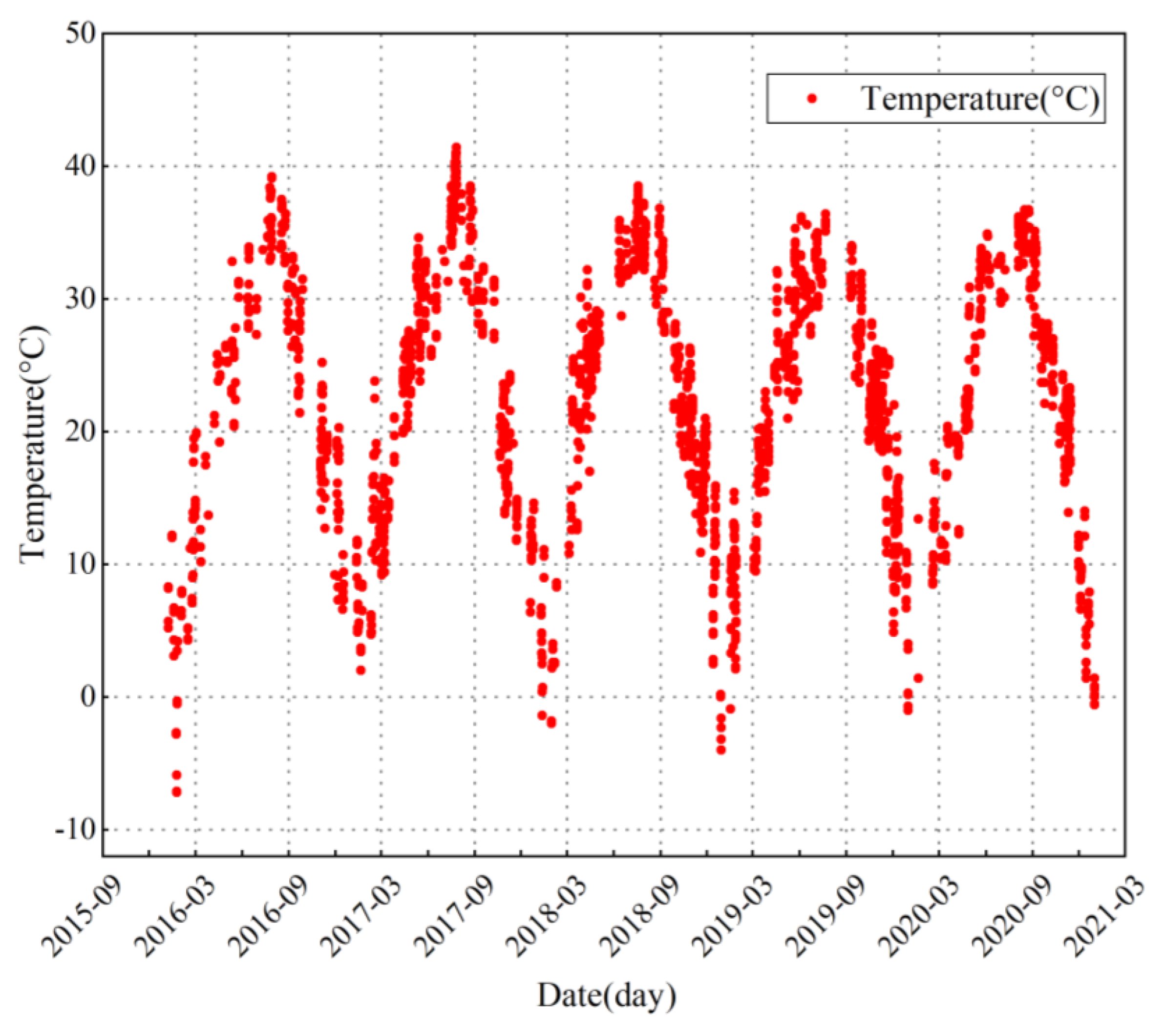
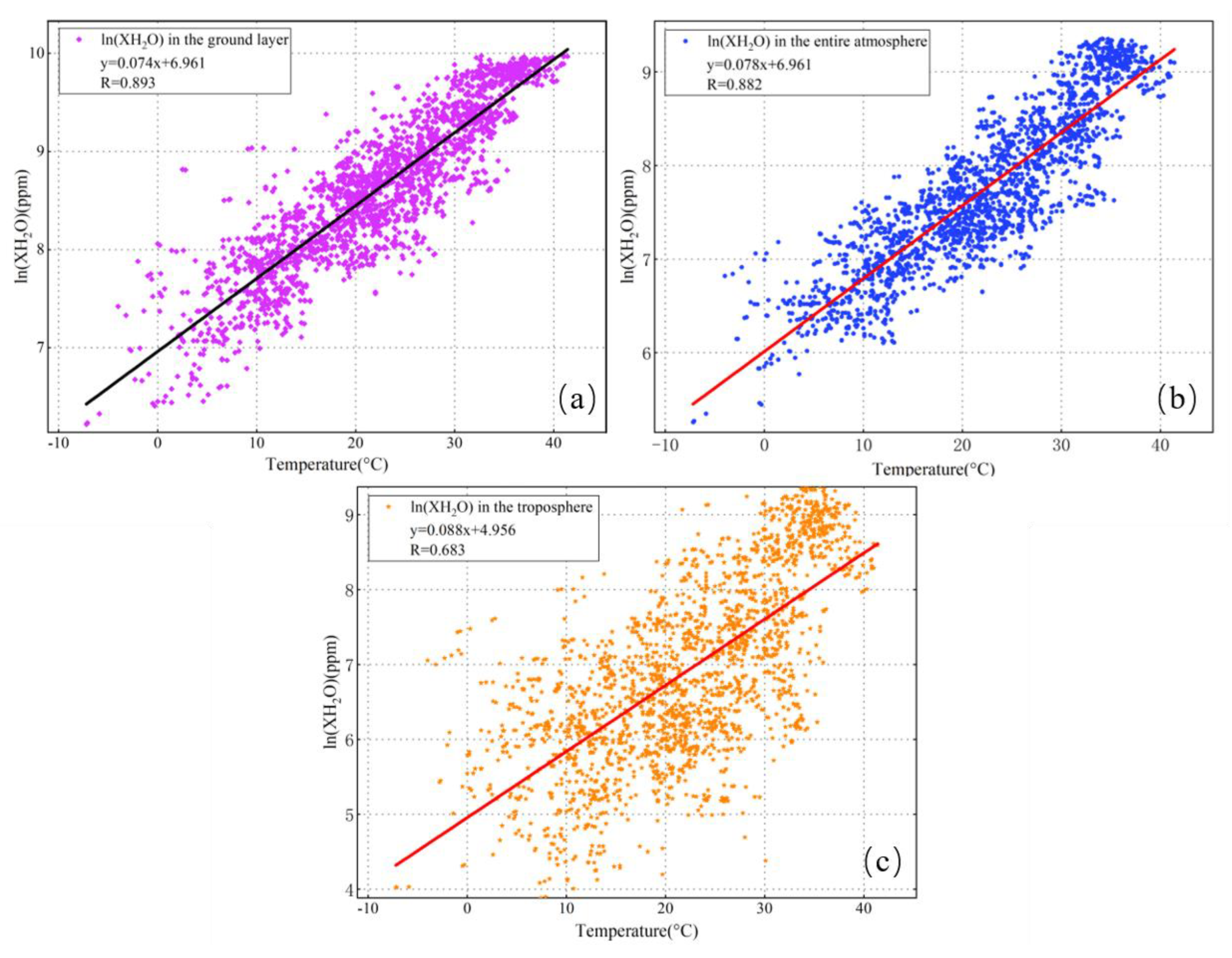
3.3. Relationship with Surface Temperature

The temperature variation has a clear influence on the seasonal variation of atmospheric H2O [20]. The spatial and temporal distribution of H2O in the atmosphere has a high correlation with weather conditions [52]. The temperature data were all obtained from the meteorological station in the Hefei site, and the time series of surface temperature from January 2016 to December 2020 is shown in Figure 14. It is found that the seasonal variation in surface temperature is similar to that of XH2O. In order to analyze the correlation between XH2O and surface temperature at the Hefei site in detail, we compared the ln(XH2O) values in the ground layer, entire atmosphere and troposphere with surface temperature from January 2016 to December 2020, respectively. Figure 15a–c illustrate the three correlations. The correlation coefficient R-value between the ground layer ln(XH2O) and temperature is 0.893, the R–value between the ln(XH2O) derived from the total column and temperature is 0.882, and the R–value between the tropospheric ln(XH2O) and temperature is 0.683. This demonstrates that the correlation between H2O columns in the ground layer and surface temperature is the highest, while the correlation of H2O columns in the troposphere with surface temperature is the weakest. Therefore, it can be seen that the temperature change is more likely to cause the change in H2O columns in the ground layer, which explains why the XH2O amplitude in the ground layer is higher than those in the entire atmosphere and the troposphere [47].

3.4. The Impact of Air Mass Transport on H2O

To understand the impact of air mass transport on H2O change in Hefei, we used the 500 m height as the starting height of the atmospheric boundary layer in the study area and simulated the 72 h backward trajectories of the air masses using the hybrid single-particle Lagrangian integrated trajectory (HYSPLIT) [53]. HYSPLIT is a comprehensive model system jointly developed by the Air Resources Laboratory of the National Oceanic and Atmospheric Administration (NOAA) of the United States and the Australian Meteorological Administration, which is used to calculate and analyze the source, transport and diffusion trajectories of atmospheric pollutants [54]. The HYSPLIT model has a relatively complete transport, diffusion and sedimentation model that can handle various meteorological input fields, physical processes and different types of pollutant emission sources. It is widely used in the study of atmospheric transport and diffusion of various pollutants in various regions [55].
The path of air mass’s impact on an area is mainly related to the position and movement law of the local pressure system, as well as the characteristics of topography and local circulation. The trajectory calculation principle of this model is based on the assumption that particles in the air move with the wind and are at the position P(t) at time t, and the position P t + Δ t after a variable time step Δ t is:
P t + Δ t = P t + 1 / 2   V P , t + V P ^ , t + Δ t Δ t
where V is the wind speed, P ^ is an intermediate conjecture position and the variable time step Δ t during the calculation process is:
P t + Δ t = P t + V P , t Δ t
We use Ward’s minimum variance method in the clustering analysis [56]. Since we only focus on the horizontal direction of air mass transportation to Hefei station, and in order to avoid Euler distance from dividing two backward trajectories with different speeds and the same path into two different categories in the calculation process, the angle distance algorithm is used to classify the air-flow trajectories to Hefei station and obtain different types of transportation air-flow [57]. Its calculation method:
d 12 = 1 n i = 1 n cos 1 1 2 A i + B i + C i A i B i
A i = X 1 i X 0 2 + Y 1 i Y 0 2
B i = X 2 i X 0 2 + Y 2 i Y 0 2
C i = X 2 i X 1 i 2 + Y 2 i Y 1 i 2
where X 0 and Y 0 is the coordinate of the starting point of the trajectory, and d 12 is the average angle between two trajectories.
The weather data used are the global data assimilation system GDAS data from 2017 to 2018 provided by the NECP, with a spatial horizontal resolution of a 0.5° × 0.5° longitude and latitude grid [58]. The backward trajectory cluster analysis was conducted in four seasons (Figure 16) based on HYSPLIT: March to May is spring, June to August is summer, September to November is autumn and December to February of the following year is winter.
The spring clusters can be divided into three types of air masses: the first type of air masses, which came from Inner Mongolia and reached Hefei via the Shanxi and Henan provinces, accounts for 24.72%; the second type of air masses, which came from Inner Mongolia and reached Hefei via the Beijing–Tianjin–Hebei region, and the Shandong and Jiangsu provinces, accounts for 37.08%. Therefore, the first 61.8% of airmasses came from dry and cold regions, which leads to low H2O values in spring. The third type of air mass accounts for 38.20% and came from the border area of the Anhui and Jiangxi provinces and went by the south of Anhui Province.
The summer clusters are divided into three air masses, with the first group accounting for 40.91% of the air masses and arriving in Hefei directly from Henan Province. The second type of air mass accounts for 21.59% and came from the Yellow Sea and entered Hefei via the Jiangsu province; the third type of air mass accounts for 37.50% and came from the South China Sea and entered Hefei via the Guangdong, Fujian and Jiangxi provinces, so the last 59.09% of airmasses came from the wet and warm regions, which leads to high H2O values in summer.
The autumn clusters are divided into three air masses, the first category with 27.91% was from Mongolia, arriving in Hefei via Inner Mongolia Province, Hebei Province, Shandong Province and Jiangsu Province; the second category with 39.53% was from Inner Mongolia Province, arriving in Hefei via the Beijing–Tianjin–Hebei region, the Yellow Sea and Jiangsu Province. Therefore, the first 61.44% of airmasses came from the dry and cold regions, which leads to low H2O values in autumn, similar to the pattern in spring. The third type of air mass comes from the border area of Anhui and Jiangxi with a percentage of 32.56%.
Winter can also be divided into three air masses; the first and second types of air masses both come from Mongolia. The first type of air masses accounts for 18.39% and reached Hefei via the Inner Mongolia, Shaanxi, Shanxi and Henan provinces, the second type of air masses accounts for 40.23% and reached Hefei via the Inner Mongolia, Shaanxi, Hebei, Shandong and Jiangsu provinces. The third type of air mass, accounting for 41.38%, came from Shandong Province and entered Hefei via Jiangsu Province. Therefore, almost 100% of airmasses came from the dry and cold regions, which leads to very low H2O values in winter.

4. Conclusions

The H2O total columns, ground-layer H2O columns and tropospheric H2O columns were retrieved from the solar absorption spectra recorded by the ground-based high-resolution FTIR at the Hefei site. The H2O total columns were retrieved from NIR and MIR spectra, respectively. The average root-mean-square deviation of fitting residuals of NIR and MIR H2O spectra are 0.16% and 0.324%, respectively. In the retrieval process of the MIR H2O column, we found that the typical DOFs for H2O over Hefei are about 2.53. Therefore, the column is divided into the ground layer and the troposphere. In addition, we conducted an error analysis on the MIR H2O column and found that the random and systematic errors are about 6.49% and 1.55%, respectively. Among them, the uncertainties of the temperature profile are the main random error and system error sources, accounting for 6.43% and 1.08%, respectively. The errors due to uncertainties of smoothing error and measurement error are very small, accounting for 0.026% and 0.05%. The systematic error of H2O is mainly determined by the uncertainty of the temperature profile.
The time series of the H2O total column and tropospheric H2O column were obtained from January 2016 to December 2020. It is clear that the trend of XH2O measured in the NIR region is similar to that measured in the MIR range, both showing obvious seasonal variations over the observation period, and having a high correlation between the two datasets (R = 0.989). The amounts of atmospheric XH2O are higher in summer than those in spring and winter, and the seasonal variations in the five years are consistent.
For ground-layer H2O columns, the amounts of XH2O reach up to the maximum of 14496.66~18365.01 ppm in each August, and the daily average XH2O reached the peak of 8713.48 ppm in August, while it is only 1277.42~2026.47 ppm for the minimum in each early spring and winter. The XH2O values in the ground layer are obviously higher than those in the entire atmosphere and troposphere, the averaged difference is 4113.64 ppm and 5292.53 ppm, respectively (the standard deviation is 2834.67 ppm and 3575.93 ppm, respectively). This is because H2O is mainly distributed below the troposphere, and H2O transpiration mainly occurs near the surface, which is related to the enhanced contribution of the moist atmosphere near the ground to the XH2O value.
The temperature variations have a strong influence on the seasonal variation of atmospheric H2O, so the relationship of H2O and surface temperature was also calculated, and it is found that the seasonal variation in temperature is similar to H2O variation. The relationship between surface temperature and ln(H2O) values in the ground layer, entire atmosphere and troposphere all show a significantly positive correlation and the correlation coefficient R-values are 0.893, 0.882 and 0.683, respectively. The change in temperature likely causes the change in H2O in the troposphere.
Further, we selected the HYSPLIT model to simulate the back trajectories of the air parcels at the Hefei site in different seasons and performed the cluster analysis. Firstly, about 61.8% of airmasses came from the dry and cold regions, which leads to low H2O values in spring. Secondly, about 59.09% of airmasses came from the wet and warm region, which leads to high H2O values in summer. Thirdly, about 61.44% of airmasses came from the dry and cold regions, which leads to low H2O values in autumn, similar to the pattern in spring. Finally, almost 100% of airmasses came from the dry and cold regions, which leads to very low H2O values in winter.
FTIR is a powerful tool for observing H2O in the atmosphere, and long-term monitoring of H2O provides the basis for unravelling the atmospheric water cycle. The combined observations of atmospheric H2O and H2O isotopes can reveal the processes of troposphere–stratosphere exchange, cloud processes, rain recycling and evapotranspiration. H2O isotopic measurements can be used to effectively distinguish the representation of processes controlling the distribution of atmospheric humidity in different models. Our future research will focus on the accurate retrieval of the H2O stable isotopes HDO, H216O and H218O from the solar absorption spectrum, which together with H2O and its stable isotopes, can clarify the atmospheric water cycle.

Author Contributions

Funding acquisition, W.W., C.L. and C.S.; resources, Y.X., Q.Z., B.L. and X.Z.; writing—original draft, P.W.; writing—review and editing, W.W. and C.S. All authors have read and agreed to the published version of the manuscript.

Funding

We gratefully acknowledge the support of the National Key Technology R&D Program of China (2022YFB3904805), the Major Projects of High Resolution Earth Observation Systems of National Science and Technology (05-Y30B01-9001-19/20-3), the Strategic Priority Research Program of the Chinese Academy of Sciences (XDA23020301), the National Key Project for Causes and Control of Heavy Air Pollution (DQGG0102 and DQGG0205), the State Environmental Protection Key Laboratory of Sources and Control of Air Pollution Complex (SCAPC202110), the Key Laboratory of Middle Atmosphere and Global environment Observation (LAGEO-2022-05), and the Funded by the Research Fund Program of Guangdong-Hongkong-Macau Joint Laboratory of Collaborative Innovation for Environmental Quality(GHML2022-002).

Data Availability Statement

The data presented in this study are available on request from the corresponding author.

Acknowledgments

We gratefully acknowledge Nicholas Jones, School of Chemistry, Wollongong University, Australia, for guidance on ground-based spectra retrieval. The processing environment of SFIT4 and some plot programs are provided by the National Center for Atmospheric Research (NCAR), Boulder, CO, USA. The NDACC network is acknowledged for supplying the SFIT software and advice.

Conflicts of Interest

The authors declare no conflict of interest.

References

  1. Trenberth, K.E. Atmospheric moisture residence times and cycling: Implications for rainfall rates and climate change. Clim. Change 1998, 39, 667–694. [Google Scholar] [CrossRef]
  2. Solomon, S.; Manning, M.; Chen, Z.; Marquis, M.; Averyt, K.B. The physical science basis: Contribution of Working Group I to the fourth assessment report of the Intergovernmental Panel on Climate Change (IPCC). Comput. Geom. 2007, 18, 95–123. [Google Scholar]
  3. Soden, B.; Wetherald, R.T.; Stenchikov, G.L.; Robock, A. Global cooling after the eruption of Mount Pinatubo: A test of climate feedback by water vapor. Science 2002, 296, 727–730. [Google Scholar] [CrossRef] [Green Version]
  4. Allan, R.P. The role of water vapour in Earth’s energy flows. Surv. Geophys. 2012, 33, 557–564. [Google Scholar] [CrossRef] [Green Version]
  5. Wood, S.W.; Batchelor, R.L.; Goldman, A.; Rinsland, C.P.; Connor, B.J.; Murcray, F.J.; Stephen, T.M.; Heuff, D.N. Ground-based nitric acid measurements at Arrival Heights, Antarctica, using solar and lunar Fourier transform infrared observations. J. Geophys. Res. 2004, 109, D18307. [Google Scholar] [CrossRef]
  6. Gong, M.; Cao, Y.; Wu, Q. A Neighborhood-Based Ratio Approach for Change Detection in SAR Images. IEEE Geosci. Remote Sens. Lett. 2012, 9, 307–311. [Google Scholar] [CrossRef]
  7. Hakim, W.L.; Achmad, A.R.; Eom, J.; Lee, C. WLand Subsidence Measurement of Jakarta Coastal Area Using Time Series Interferometry with Sentinel-1 SAR Data. J. Coastal Res. 2020, 102, 75–81. [Google Scholar] [CrossRef]
  8. Kang, M.S.; Baek, J.M. SAR Image Reconstruction via Incremental Imaging with Compressive Sensing. IEEE Trans. Aerosp. Electron. Syst. 2023, 1–14. [Google Scholar] [CrossRef]
  9. Frankenberg, C.; Yoshimura, K.; Warneke, T.; Aben, I.; Butz, A.; Deutscher, N.; Griffith, D.; Hase, F.; Notholt, J.; Schneider, M.; et al. Dynamic processes governing lower-tropospheric HDO/H2O ratios as observed from space and ground. Science 2009, 325, 1374–1377. [Google Scholar] [CrossRef]
  10. Ross, R.J.; Elliott, W.P. Tropospheric water vapor climatology and trends over North America: 1973–93. J. Clim. 1996, 9, 3561–3574. [Google Scholar] [CrossRef]
  11. Alvarado, M.J.; Payne, V.H.; Mlawer, E.J.; Uymin, G.; Moncet, J.L. Performance of the Line-By-Line Radiative Transfer Model (LBLRTM) for temperature, water vapor, and trace gas retrievals: Recent updates evaluated with IASI case studies. Atmos. Chem. Phys. 2013, 13, 6687–6711. [Google Scholar] [CrossRef] [Green Version]
  12. Ohyama, H.; Kawakami, S.; Shiomi, K.; Morino, I.; Uchino, O. Intercomparison of XH2O Data from the GOSAT TANSO-FTS (TIR and SWIR) and Ground-Based FTS Measurements: Impact of the Spatial Variability of XH2O on the Intercomparison. Remote Sens. 2017, 9, 64. [Google Scholar] [CrossRef] [Green Version]
  13. Ortega, I.; Buchholz, R.R.; Hall, E.G.; Hurst, D.F.; Jordan, A.F.; Hannigan, J.W. Tropospheric water vapor profiles obtained with FTIR: Comparison with balloon-borne frost point hygrometers and influence on trace gas retrievals. Atmos. Meas. Tech. 2019, 12, 873–890. [Google Scholar] [CrossRef] [Green Version]
  14. Dupuy, E.; Morino, I.; Deutscher, N.M.; Yoshida, Y.; Uchino, O.; Connor, B.J.; Maziere, M.D.; Griffith, D.W.T.; Hase, F.; Heikkinen, P.; et al. Comparison of XH2O retrieved from GOSAT short-wavelength infrared spectra with observations from the TCCON network. Remote Sens. 2016, 8, 414. [Google Scholar] [CrossRef] [Green Version]
  15. Schneider, M.; Hase, F.; Blumenstock, T. Water vapour profiles by ground-based FTIR spectroscopy: Study for an optimised retrieval and its validation. Atmos. Chem. Phys. 2006, 6, 811–830. [Google Scholar] [CrossRef] [Green Version]
  16. Barthlott, S.; Schneider, M.; Hase, F.; Blumenstock, T.; Robinson, J. Tropospheric water vapour isotopologue data (H216O, H218O, and HD16O) as obtained from NDACC/FTIR solar absorption spectra. Earth. Sys. Sci. Data 2017, 9, 15–29. [Google Scholar] [CrossRef] [Green Version]
  17. Vogelmann, H.; Sussmann, R.; Trickl, T.; Reichert, A. Spatiotemporal variability of water vapor investigated using lidar and FTIR vertical soundings above the Zugspitze. Atmos. Chem. Phys. 2015, 15, 3135–3148. [Google Scholar] [CrossRef] [Green Version]
  18. Wunch, D.; Wennberg, P.O.; Osterman, G.; Fisher, B.; Eldering, A. Comparisons of the Orbiting Carbon Observatory-2 (OCO-2) XCO2 measurements with TCCON. Atmos. Meas. Tech. 2017, 10, 2209–2238. [Google Scholar] [CrossRef] [Green Version]
  19. Makarova, M.V.; Serdyukov, V.I.; Arshinov, M.Y.; Voronin, B.A.; Belan, B.D.; Sinitsa, L.N.; Polovtseva, E.R.; Vasilchenko, S.S.; Kabanov, D.M. First results of ground-based Fourier Transform Infrared measurements of the H2O total column in the atmosphere over West Siberia. Int. J. Remote Sens. 2014, 35, 5637–5650. [Google Scholar]
  20. Virolainen, Y.A.; Timofeyev, Y.M.; Kostsov, V.S.; Lonov, D.V.; Blumenstock, T. Quality assessment of integrated water vapour measurements at the St. Petersburg site, Russia: FTIR vs. MW and GPS techniques. Atmos. Meas. Tech. 2017, 10, 4521–4536. [Google Scholar] [CrossRef] [Green Version]
  21. Tu, Q.; Hase, F.; Blumenstock, T.; Schneider, M.; Schneider, A.; Kivi, R.; Heikkinen, P.; Ertl, B.; Diekmann, C.; Khosrawi, F.; et al. Intercomparison of Arctic ground-based XH2O observations from COCCON, TCCON and NDACC, and application of COCCON XH2Ofor IASI and TROPOMI validation. Atmos. Meas. Tech. 2021, 14, 1993–2011. [Google Scholar] [CrossRef]
  22. Shan, C.; Wang, W.; Liu, C.; Guo, Y.; Jones, N. Retrieval of vertical profiles and tropospheric CO2 columns based on high-resolution FTIR over Hefei, China. Opt. Express. 2021, 29, 4958–4977. [Google Scholar] [CrossRef]
  23. Shan, C.; Wang, W.; Liu, C.; Sun, Y.; Hu, Q.; Xu, X.; Tian, Y.; Zhang, H.; Morino, I.; Griffith, D.W.T.; et al. Regional CO emission estimated from ground-based remote sensing at Hefei site, China. Atmos. Res. 2019, 222, 25–35. [Google Scholar] [CrossRef] [Green Version]
  24. Wang, W.; Tian, Y.; Liu, C.; Sun, Y.W.; Liu, W.; Xie, P.; Liu, J.; Xu, J.; Morino, I.; Griffith, D.W.; et al. Investigating the performance of a greenhouse gas observatory in Hefei, China. Atmos. Meas. Tech. 2017, 10, 2627–2643. [Google Scholar] [CrossRef] [Green Version]
  25. Hase, F.; Drouin, B.J.; Roehl, C.M.; Toon, G.C.; Wennberg, P.O.; Wunch, D.; Blymenstock, T.; Desmet, F.; Feist, D.G.; Heikkinen, P.; et al. Calibration of sealed HCl cells used for TCCON instrumental line shape monitoring. Atmos. Meas. Tech. 2013, 6, 3527–3537. [Google Scholar] [CrossRef] [Green Version]
  26. Sun, Y.; Liu, C.; Palm, M.; Vigouroux, J.; Hu, Q.; Jones, N.; Wang, W.; Zhang, W. Ozone seasonal evolution and photochemical production regime in the polluted troposphere in eastern China derived from high-resolution Fourier transform spectrometry (FTS) observations. Atmos. Chem. Phys. 2018, 18, 14569–14583. [Google Scholar] [CrossRef] [Green Version]
  27. Wunch, D.; Toon, G.C.; Wennberg, P.O.; Wofsy, S.C.; Stephens, B.B. Calibration of the Total Carbon Column Observing Network using aircraft profile data. Atmos. Meas. Tech. 2010, 3, 1351–1362. [Google Scholar] [CrossRef] [Green Version]
  28. Tanaka, T.; Miyamoto, Y.; Morino, I.; Machida, T.; Nagahama, T. Aircraft measurements of carbon dioxide and methane for the calibration of ground-based high-resolution Fourier Transform Spectrometers and a comparison to GOSAT data measured over Tsukuba and Moshiri. Atmos. Meas. Tech. 2012, 5, 1843–1871. [Google Scholar] [CrossRef] [Green Version]
  29. Borsdorff, T.; Hu, H.; Hasekamp, O.; Sussmann, R.; Rettinger, M.; Hase, F.; Gross, J.; Schneider, M.; Garcia, O. Mapping carbon monoxide pollution from space down to city scales with daily global coverage. Atmos. Meas. Tech. 2018, 11, 5507–5518. [Google Scholar] [CrossRef] [Green Version]
  30. Kalnay, E.; Kanamitsu, M.; Kistler, R.; Collins, W.; Deaven, D.; Gandin, L.; Iredell, M.; Saha, S.; White, G.; Woollen, J. The NCEP/NCAR 40-year Reanalysis project. Bull. Am. Meteorol. Soc. 1996, 77, 437–471. [Google Scholar] [CrossRef]
  31. Rothman, L.S.; Gordon, I.E.; Barbe, A.; Benner, D.C.; Bernath, P.F.; Birk, M.; Boidon, V.; Brown, L.R.; Campargue, A.; Champion, J.P.; et al. The HITRAN 2008 molecular spectroscopic database. J. Quant. Spectrosc. Radiat. Transf. 2009, 110, 533–572. [Google Scholar] [CrossRef] [Green Version]
  32. Wunch, D.; Toon, G.C.; Blavier, J.F.; Washenfelder, R.A.; Notholt, J.; Connor, B.J.; Griffith, D.W.; Sherlock, V.; Wennberg, P.O. Thetotal carbon column observing network. Philos. Trans. A Math. Phys. Eng. Sci. 2011, 369, 2087–2112. [Google Scholar]
  33. Zhou, M.; Dils, B.; Wang, P.; Detmers, R.; Maziere, M.D. Validation of TANSO-FTS/GOSAT XCO2 and XCH4 glint mode retrievals using TCCON data from near-ocean sites. Atmos. Meas. Tech. 2016, 9, 1415–1430. [Google Scholar] [CrossRef] [Green Version]
  34. Pougatchev, N.S.; Connor, B.J.; Rinsland, C.P. Infrared measurements of the ozone vertical distribution above Kitt Peak. J. Geophys. Res. Atmos. 1995, 100, 16689–16697. [Google Scholar] [CrossRef] [Green Version]
  35. Timofeyev, Y.; Virolainen, Y.; Makarova, M.; Poberovsky, A.; Polyakov, A.; Lomov, D.; Osipov, S.; Lmhasin, H. Ground-based spectroscopic measurements of atmospheric gas composition near Saint Petersburg (Russia). J. Mol. Spectrosc. 2016, 323, 2–14. [Google Scholar] [CrossRef]
  36. García, O.E.; Schneider, M.; Sepúlveda, E. Twenty years of ground-based NDACC FTIR spectrometry at Izaña Observatory–overview and long-term comparison to other techniques. Atmos. Chem. Phys. 2021, 21, 15519–15554. [Google Scholar] [CrossRef]
  37. Sorrel, M. The NCEP climate forecast system reanalysis. Bull. Am. Meteorol. Soc. 2010, 91, 1015–1058. [Google Scholar]
  38. Rothman, L.S.; Gordon, I.E.; Babikov, Y.; Benner, A.C.; Bernath, D.; Birk, P.F.; Bizzocchi, M.; Boudon, L.; Brown, V.; Campargue, L.R. The HITRAN2012 molecular spectroscopic database. J. Quant. Spectrosc. Radiat. Transf. 2013, 130, 4–50. [Google Scholar] [CrossRef] [Green Version]
  39. Rodgers, C.D.; Connor, B.J. Intercomparison of remote sounding instruments. J. Geophys. Res. Atmos. 2003, 108, 4116–4229. [Google Scholar] [CrossRef] [Green Version]
  40. Zeng, X.; Wang, W.; Liu, C.; Shan, C.; Xie, Y.; Wu, P.; Zhu, Q.; Zhou, M.; Mahieu, E. Retrieval of atmospheric CFC-11 and CFC-12 from high-resolution FTIR observations at Hefei and comparisons with other independent datasets. Atmos. Meas. Tech. 2022, 15, 6739–6754. [Google Scholar] [CrossRef]
  41. Schneider, M.; Wiegele, A.; Barthlott, S.; González, Y.; Christner, E.; Dyroff, C.; García, O.E.; Hase, F.; Blumenstock, T.; Sepúlveda, E. Accomplishments of the MUSICA project to provide accurate, long-term, global and high-resolution observations of tropospheric { H2O, δD} pairs–A review. Atmos. Meas. Tech. 2016, 9, 2845–2875. [Google Scholar] [CrossRef] [Green Version]
  42. García, O.E.; Schneider, M.; Redondas, A.; González, Y.; Hase, F.; Blumenstock, T.; Sepúlveda, E. Investigating the long-term evolution of subtropical ozone profiles applying ground-based FTIR spectrometry. Atmos. Meas. Tech. 2012, 5, 2917–2931. [Google Scholar] [CrossRef] [Green Version]
  43. Schneider, M.; Hase, F.; Blavier, J.F.; Toon, G.C.; Leblanc, T. An empirical study on the importance of a speed-dependent Voigt line shape model for tropospheric water vapor profile remote sensing. J. Quant. Spectrosc. Radiat. Transf. 2011, 112, 465–474. [Google Scholar] [CrossRef]
  44. Schneider, M.; Barthlott, S.; Hase, F.; González, Y.; Yoshimura, K. Ground-based remote sensing of tropospheric water vapour isotopologues within the project MUSICA. Atmos. Meas. Tech. 2012, 5, 3007–3027. [Google Scholar] [CrossRef] [Green Version]
  45. Kiel, M.; Hase, F.; Blumenstock, T.; Kirner, O. Comparison of XCO abundances from the Total Carbon Column Observing Network and the Network for the Detection of Atmospheric Composition Change measured in Karlsruhe. Atmos. Meas. Tech. 2016, 9, 2223–2239. [Google Scholar] [CrossRef] [Green Version]
  46. Reuter, M.; Bovensmann, H.; Buchwitz, M.; Burrows, J.P.; Connor, J.B.; Deutscher, N.M.; Griffith, D.W.T.; Heymann, J.; Keppel-Aleks, G.; Messerschmidt, J. Retrieval of atmospheric CO2 with enhanced accuracy and precision from SCIAMACHY: Validation with FTS measurements and comparison with model results. J. Geophys. Res. Atmos. 2011, 116, D04301. [Google Scholar] [CrossRef] [Green Version]
  47. Noone, D. Pairing measurements of the water vapor isotope ratio with humidity to deduce atmospheric moistening and dehydration in the tropical midtroposphere. J. Clim. 2012, 25, 4476–4494. [Google Scholar] [CrossRef]
  48. Vogelmann, H.; Sussmann, R.; Trickl, T.; Borsdorff, T. Intercomparison of atmospheric water vapor soundings from the differential absorption lidar (DIAL) and the solar FTIR system on Mt. Zugspitze. Atmos. Meas. Tech. 2011, 4, 835–841. [Google Scholar] [CrossRef] [Green Version]
  49. Shan, C.; Zhang, H.; Wang, W.; Liu, C.; Xie, Y.; Hu, Q.; Jones, N. Retrieval of Stratospheric NO3 and HCl Based on Ground-Based High-Resolution Fourier Transform Spectroscopy. Remote Sens. 2021, 13, 2159. [Google Scholar] [CrossRef]
  50. Shan, C.; Wang, W.; Xie, Y.; Wu, P.; Xu, J.; Zeng, X.; Zha, L.; Zhu, Q.; Sun, Y.; Hu, Q.; et al. Observations of atmospheric CO2 and CO based on in-situ and ground-based remote sensing measurements at Hefei site, China. Sci. Total Environ. 2022, 851, 158188. [Google Scholar] [CrossRef] [PubMed]
  51. Tu, M.; Zhang, W.; Bai, J. Spatio-Temporal Variations of Precipitable Water Vapor and Horizontal Tropospheric Gradients from GPS during Typhoon Lekima. Remote Sens. 2021, 13, 4082. [Google Scholar] [CrossRef]
  52. Pistone, K.; Zuidema, P.; Wood, R.; Diamond, M.; Shinozuka, Y. Exploring the elevated water vapor signal associated with the free-tropospheric biomass burning plume over the southeast Atlantic Ocean. Atmos. Chem. Phys. 2021, 21, 9643–9668. [Google Scholar] [CrossRef]
  53. King, M.D.; Menzel, W.P.; Kaufman, Y.J.; Tanré, D.; Hubanks, P.A. Cloud and aerosol properties, precipitable water, and profiles of temperature and water vapor from MODIS. IEEE Trans. Geosci. Remote Sens. 2003, 41, 442–458. [Google Scholar] [CrossRef] [Green Version]
  54. Fan, Q.; Zhang, Y.; Ma, W.; Ma, H.; Feng, J.; Qi, Y.; Yang, X.; Fu, Q.; Liu, C. Spatial and Seasonal Dynamics of Ship Emissions over the Yangtze River Delta and East China Sea and Their Potential Environmental Influence. Environ. Sci. Technol. 2016, 50, 1322–1329. [Google Scholar] [CrossRef] [PubMed]
  55. Draxler, R.R.; Hess, G.D. An overview of the HYSPLIT_4 modeling system of trajectories, dispersion, and deposition. Aust. Meteorol. Mag. 1998, 47, 295–308. [Google Scholar]
  56. Szekely, G.J.; Rizzo, M.L. Hierarchical Clustering via Joint Between-Within Distances: Extending Ward’s Minimum Variance Method. J. Classif. 2005, 22, 151–183. [Google Scholar] [CrossRef]
  57. Siroris, A.; Bottenheim, J.W. Use of backward trajectories to interpret the 5-year record of PAN and O3 ambient air concentrations at Kejimkujik National Park, Nova Scotia. J. Geophys. Res. Atmos. 1995, 100, 2867–2881. [Google Scholar] [CrossRef]
  58. Brankov, E.; Rao, S.T.; Porter, P.S. A trajectory-clustering-correlation methodology for examining the long-range transport of air pollutants. Atmos. Environ. 1998, 32, 1525–1534. [Google Scholar] [CrossRef]
Figure 1. FTIR instrument for measurements at the Hefei site. (a) Bruker 125HR FTIR spectrometer placed indoors; (b) solar tracker placed outdoors.
Remotesensing 15 03484 g001
Figure 2. The fitting results of H2O in NIR region. The red lines are the calculated spectra, the black lines are the measured spectra, the blue lines are the absorption signals for H2O, the bottom panels are the spectra–fitting residuals.
Remotesensing 15 03484 g002
Figure 3. Column averaging kernels of H2O.
Remotesensing 15 03484 g003
Figure 4. The spectral fitting of H2O in the four micro–windows. The red lines are the calculated spectra, the blue lines are the observed spectra, and the upper panels are the spectra fitting residuals. (a) shows the spectral fitting of H2O in the 2732.28–2732.82 cm 1 micro–window. (b) shows the spectral fitting of H2O in the 2818.80–2820.13 cm 1 micro–window. (c) shows the spectral fitting of H2O in the 2878.55–2880.65 cm 1 micro–window. (d) shows the spectral fitting of H2O in the 2878.55–2880.65 cm 1 micro–window.
Remotesensing 15 03484 g004
Figure 5. Measured H2O profiles and a priori profiles observed from 2016 to 2020 at the Hefei site. The blue shaded area is the 1− σ standard deviation, the red line is the averaged retrieved profile, and the black dotted line is the a priori profile.
Remotesensing 15 03484 g005
Figure 6. Typical averaging kernels of retrieved H2O profile, sensitivity is plotted with the dashed line.
Remotesensing 15 03484 g006
Figure 7. Typical signal degree of freedom of H2O.
Remotesensing 15 03484 g007
Figure 8. Time series of daily averaged XH2O obtained from NIR and MIR spectra. The blue dots are the daily averaged XH2O obtained from the MIR spectra, the yellow dots are the daily averaged XH2O obtained from the NIR spectra, the error bars are the standard deviations of the daily averaged XH2O. Differences between the coincident data pairs are presented in the top panel.
Remotesensing 15 03484 g008
Figure 9. Correlation diagram of XH2O in the NIR and MIR spectra. The bar chart on the right represents the month.
Remotesensing 15 03484 g009
Figure 10. Time series of daily averaged XH2O in the ground layer and in the entire atmosphere. The purple dots are the daily averaged XH2O in the ground layer, the green dots are the daily averaged XH2O in the entire atmosphere, the red line is the fitting curve, the error bars are the standard deviations of the daily averaged XH2O. The differences between the coincident daily averaged XH2O data pairs are presented in the top panel.
Remotesensing 15 03484 g010
Figure 11. Correlation diagram of the XH2O in the ground layer and the entire atmosphere. The bar chart on the right represents the month.
Remotesensing 15 03484 g011
Figure 12. Time series of XH2O in the ground layer and the troposphere. The purple dots are the daily averaged XH2O in the ground layer, the orange dots are the daily averaged XH2O in the troposphere, the red line is the fitting curve, the error bars are the standard deviations of the daily averaged XH2O. The differences between the coincident daily averaged XH2O data pairs are presented in the top panel.
Remotesensing 15 03484 g012
Figure 13. Correlation diagram of the XH2O in the ground layer and troposphere. The bar chart on the right represents the month.
Remotesensing 15 03484 g013
Figure 14. Time series of surface temperature from January 2016 to December 2020.
Remotesensing 15 03484 g014
Figure 15. Relationship of ln(XH2O) in the ground layer, entire atmosphere and troposphere and surface temperature from January 2016 to December 2020 is depicted in (ac).
Remotesensing 15 03484 g015
Figure 16. Cluster analysis of airmass backward trajectories in each season at Hefei station. The colorful line represents the cluster analysis result. (a) shows the cluster analysis of airmass backward trajectories in spring. (b) shows the cluster analysis of airmass backward trajectories in summer. (c) shows the cluster analysis of airmass backward trajectories in autumn. (d) shows the cluster analysis of airmass backward trajectories in winter.
Remotesensing 15 03484 g016
Table 1. The parametric indices of the instrument and spectral data.
Instrument ParametricNIR SpectraMIR Spectra
Spectral range4000–11,000 cm−1600–4500 cm−1
Spectral resolution0.02 cm−10.005 cm−1
Optical path difference45 cm180 cm
Beam splitterCaF2KBr
DetectorInGaAsInSb/MCT
ILSHClHBr
Table 2. The parameters for NIR H2O retrieval.
Center of Spectral
Window   ( c m 1 )
Width   ( c m 1 ) Interfering Gas
H2O4571.752.50 H 2 O , CO 2 , CH 4
4611.052.20 H 2 O , CO 2 , CH 4 , N 2 O
4699.554.00 H 2 O , CO 2 , N 2 O
6076.903.85 H 2 O , CO 2 , CH 4 , HDO
6125.851.45 H 2 O , CO 2 , CH 4 , HDO
6255.953.60 H 2 O , CO 2 , HDO
6301.357.90 H 2 O , CO 2 , HDO
6392.453.10 H 2 O , HDO
6401.151.15 H 2 O , CO 2 , HDO
6469.603.50 H 2 O , CO 2 , HDO
Table 3. The parameters for MIR H2O retrieval.
SpeciesH2O
Retrieval softwareSFIT4 V0.9.4.4
SpectroscopyHITRAN 2012
Temperature, pressure and H2O profiles NECP
A priori profiles of retrieved speciesWACCM v6
Spectral windows ( cm 1 )2732.28–2732.82
2818.80–2820.13
2878.55–2880.65
2892.83–2893.25
Interfering gasesCH4, N2O, O3, HCl
Table 4. Random uncertainty and systematic uncertainty in the error analysis.
ParameterRandom UncertaintySystematic Uncertainty
Temperature profile3K3K
Solar zenith angle0.025°0.025°
Solar line shift0.005 cm 1 0.005 cm 1
Solar line strength0.1%0.1%
Field of view0.010.01
Line intensity-1%
Line T broadening-10%
Line P broadening-3%
Spectroscopic parameters2%2%
Table 5. Mean random and systematic errors for H2O retrieval.
ParameterRandom Error/%Systematic Error/%
Smoothing error0.026-
Measurement error0.05-
Temperature profile6.431.08
Solar zenith angle0.0490.049
Zero level shift0.720.72
Field of view0.0170.017
Line intensity-0.083
Line T broadening0.0230.023
Line P broadening0.9640.964
Spectroscopic parameters0.9680.968
Subtotal error6.491.55
Total error6.67
Disclaimer/Publisher’s Note: The statements, opinions and data contained in all publications are solely those of the individual author(s) and contributor(s) and not of MDPI and/or the editor(s). MDPI and/or the editor(s) disclaim responsibility for any injury to people or property resulting from any ideas, methods, instructions or products referred to in the content.

