Article

Seasonal and Diurnal Changes of Air Temperature and Water Vapor Observed with a Microwave Radiometer in Wuhan, China

1
School of Electronic Information, Wuhan University, Wuhan 430072, China
2
Key Laboratory of Geospace Environment and Geodesy, Ministry of Education, Wuhan 430072, China
3
State Observatory for Atmospheric Remote Sensing, Wuhan 430072, China
*
Author to whom correspondence should be addressed.
Remote Sens. 2023, 15(22), 5422; https://doi.org/10.3390/rs15225422
Submission received: 26 October 2023 / Revised: 12 November 2023 / Accepted: 17 November 2023 / Published: 20 November 2023
(This article belongs to the Special Issue Remote Sensing of Atmospheric Composition)

Abstract

:
Based on Microwave Radiometer (MWR) observations in Wuhan over the course of 21 months, we compared the temperature and water vapor levels with those from radiosonde (RS) sounding data at 00:00 and 12:00 UTC, and then analyzed the seasonal and diurnal changes of temperature and water vapor levels from the MWR data. The MWR and RS mean temperatures and dew points are roughly consistent with each other below 2 km, whereas above 2 km, the MWR temperature is slightly lower than the RS temperature. The difference in their water vapor densities decreases quickly with height, and the bias of their relative humidities is generally in the range of −15% to 20%. The MWR observations show that in autumn, the surface temperature is 6.8 K lower during precipitation events than during non-precipitation events, indicating that precipitation in autumn is mainly caused by cold air from the north. The relative humidity during precipitation events exceeds 90% from the ground to 5 km, which is obviously larger than during non-precipitation events. During non-precipitation events, the seasonal mean water vapor density at 0–1.0 km shows an approximately linear increase with the mean temperature; however, their diurnal changes are opposite due to the effect of the boundary layer. At 4.5–5.5 km and 8.5–9.5 km, the mean temperature shows a synchronized diurnal evolution, with the maximum value prior to that at 0–1.0 km, indicating the strong influence of the air–land interaction on the temperature near the ground. Hence, this study is helpful for deepening our understanding of temperature and humidity variabilities over Wuhan.

1. Introduction

Temperature is a key parameter of the atmosphere that represents the thermodynamic state of the atmosphere [1]. The large-scale movement of the atmosphere depends on the temperature gradient, and the phase transition of water vapor is closely related to temperature changes; thus, the temperature is both an essential basis and an important component of the weather forecast. As a main greenhouse gas, water vapor plays a crucial role not only in the energy budget of the local atmosphere, by absorbing solar and surface radiation, releasing latent heat during phase transition, and reflecting radiation indirectly through cloud formation, but also in the energy balance of the global atmospheric system, through its horizontal and vertical transport [2,3]. Water vapor is the core constituent of weather changes, such as clouds, fog, rain, snow, frost, dew, etc., and an important factor of climate change [4]. There is a complex interplay between the air temperature and water vapor content. The temperature can regulate the water vapor content and distribution by controlling surface evapotranspiration, saturation vapor pressure, and the horizontal and vertical motion of air, while water vapor can impact the temperature variation through its effect on the energy budget and its global transport by the circulation of the atmosphere [5,6,7,8]. Hence, it is of significance to investigate the variations of temperature and water vapor and their relationship.
The radiosonde (RS) device is an effective means to measure air temperature and humidity, and a large number of RS devices around the world are released to obtain meteorological data at 00:00 and 12:00 UTC (Coordinated Universal Time). As the balloon rises, sensors on board precisely sense the temperature and humidity from the surface to the lower stratosphere with fine vertical resolution. There are some inherent measurement errors in the RS measurements due to daytime solar radiation, the time lag of the thermistor and hygristor, and the effect of real-time wind on the sounding balloon [9,10,11,12].
Satellite observations have good spatial coverage; these observations are suitable for studying the global distribution and large-scale evolution of temperature and water vapor [13,14,15]. It has been proposed that the uncertainties in temperature and specific humidity measurements using satellite infrared and microwave sounding techniques depend on the surface and cloud properties in the footprints [16,17]. In spite of their own advantages, the low time resolution of RS and satellite data, due to only one or two samples a day over one site, constrains the investigation of the diurnal evolution of temperature and water vapor, and even the daily and monthly average values.
As a typical ground-based passive remote sensing device, the Microwave Radiometer (MWR) was developed to obtain the profiles of temperature and water vapor from the surface to about 10 km with a high temporal resolution of about 1–5 min; thus, the MWR has the ability to continuously monitor the temperature and humidity of the atmosphere with relative high accuracy [18,19,20]. The MWR measures the brightness temperature at multiple microwave channels to retrieve the profiles of the air temperature, water vapor, and liquid water. The retrieval techniques generally include the linear and nonlinear regression algorithms and artificial neural networks [21,22,23]. The artificial neural network algorithm is extensively applied to derive temperature and humidity measurements due to its high accuracy [24,25]. Many works have examined the observed profiles from the MWR in comparison with those from RS devices [26,27,28,29]. In the lower atmosphere, the annual mean temperature from the MWR is largely consistent with that from RS devices, whereas, except at the layer near the ground, the MWR mean temperature is usually lower than the RS average, and their bias generally increases with height, and may attain 3–6 K at 10 km [30,31,32]. The comparison between the relative humidities measured by the MWR and RS devices indicated that their bias is generally in the range of −25–25% at different sites. Meanwhile, the bias magnitudes may be closely related to long-term drifts, MWR site terrains, and weather conditions [30,33,34,35,36]; nevertheless, some studies have showed that MWR can perform well with sufficient accuracy during rainfall, snowfall, and in cloudy conditions [19,31,37,38]. The MWR may benefit further from improving the retrieval model and training retrieval coefficients in complex terrains and various weather conditions by minimizing the uncertainty in simulated brightness temperatures.
MWR observations have been widely used to study thermodynamic structures and weather processes. By combining MWR, ceilometer, and lidar measurements, the heights of the convective boundary layer during the daytime and the stable boundary layer during the nighttime were calculated and compared with each other [39,40,41], and the spatial and temporal variabilities of air temperature and humidity at different sites were discussed [42,43,44,45,46,47]. MWR data were helpful in diagnosing the macrophysical and microphysical properties of clouds and precipitation and estimating the rainfall rate [19,20,30,48,49], and forecasting convective activity [50,51]. Owing to the high temporal resolution, the observations of the MWR and wind profile radar were applied to the investigation of fog, which improved the understanding of atmospheric conditions for the formation, development, and dissipation of fog [32,52,53]. In addition, some studies adopted the MWR to estimate and calibrate other equipment measurements [18,54,55]. In light of the effect of water vapor on atmospheric transmittance in near real time derived from the MWR absolute humidity and temperature profiles, the ceilometer signal below 1 km was found to be overestimated up to 9% [18].
In this paper, we use the MWR observations at a mid-latitude site to investigate the seasonal and diurnal evolutions of air temperature and humidity and discuss their relevancy, which is helpful for improving our understanding of temperature and water vapor environments in the mid-latitude inland monsoon region. In Section 2, the MWR and the data used are briefly described. Section 3 presents a comparison of air temperature and humidity between the MWR and RS observations in order to evaluate the MWR measurements. In Section 4, we roughly estimate the temperature and water vapor levels during precipitation events from the MWR measurements and analyze in detail the seasonal and diurnal variations of temperature and humidity over Wuhan. Section 5 provides a summary.

2. Instruments, Data and Method

An MWR MP-3000A is placed at the Atmospheric Remote Sensing Observatory (ARSO) in Wuhan University (30.5°N, 114.4°E, 50 m above sea level), and is installed on the roof of the ARSO, as shown in Figure 1. As an inland megacity in central China, Wuhan is located on the eastern edge of the Jianghan Plain, or the transition zone from the Plain to the hills, and is dominated by the subtropical monsoon climate, with abundant precipitation, sufficient heat, and four distinct seasons. With an area of 3.5 km2, Wuhan University is adjacent to East Lake that covers 31.8 km2 of water, which may contribute to the humid air over the campus, especially in the hot summer.

2.1. MWR MP-3000A

The MWR MP-3000A, built by Radiometrics Inc., Boulder, USA, obtains air temperature and water vapor information by automatically scanning at two operating frequency bands. The MWR can sequentially observe the atmospheric radiation intensity or brightness temperature using 14 oxygen channels in the V-band (51–59 GHz) along the side of the oxygen feature at 60 GHz. The emission at any altitude is proportional to the local temperature and oxygen density, and air temperature (T) from the surface to 10 km can be retrieved by solving the microwave radiation transfer equation based on the backward propagation neural network algorithm [56]. In this study, the backward propagation neural network algorithm was trained by using a 5-year historical RS data set from the same location in the period of 2015–2019. The MWR measures the intensity and shape of the emission spectrum from pressure-broadened water vapor lines near 22 GHz sampled by 21 channels in the K-band (22–30 GHz). The intensity of the emission spectrum is proportional to the water vapor density (VD) and temperature; thus, the water vapor profile can be obtained by scanning the spectral profile and then mathematically inverting the observed data. Air temperature and water vapor are recorded every two minutes at 58 levels, with 50 m steps to 0.5 km, 100 m steps to 2 km, and 250 m steps to 10 km. By measuring the contribution of cloud liquid water to atmospheric spectral features of varying opacity, cloud liquid information in the K-band and V-band is used to obtain the liquid profile. To obtain reliable data, the MWR at the ARSO was calibrated every three months by using cold liquid nitrogen and tipping-curve calibration methods [57]. In the case of snow conditions, the snow tends to freeze and is not easily blown away by the blower system, and we generally carried out the manual removal of snow that froze on the top of the radome in winter, although this rarely took place in Wuhan.
The MWR began collecting the data on 7 December 2020; nevertheless, valid observations are missing between December 2021 and August 2022 due to maintenance difficulties during the pandemic. Thus, we investigate the seasonal and diurnal variations of temperature and water vapor over Wuhan based on the MWR observation from 7 December 2020 to 31 May 2023 when data are available.

2.2. Radiosonde Data

RS devices can obtain data for many meteorological parameters, such as temperature, pressure, water vapor mixing ratio, relative humidity, dew point, and wind speed and direction, which are generally accepted as reliable observations for comparison with those of other instruments. Here, the profiles of temperature, water vapor density, relative humidity, and dew point from the RS observations at the Wuhan station are utilized to compare with those from the MWR observations. RS devices are launched twice a day at 00:00 and 12:00 UTC, corresponding to 8:00 and 20:00 LT (Local Time) in Wuhan, and all data are analyzed in LT in the following investigation. The RS data can be downloaded from the University of Wyoming at the website of http://weather.uwyo.edu/upperair/sounding.html. The Wuhan RS station (30.6°N, 114.1°E, 23 m above sea level) is located in the northwest suburbs of Wuhan City, with an open and flat terrain, whereas Wuhan University is in the east of Wuhan City; thus, the two sites are about 50 km apart. RS data are generally presented from an altitude of nearly 200 m above sea level (ASL); thus, when we take the 50-m altitude of the MWR as the starting height, the comparative analysis starts with the height of 150 m.
The RS data in Wuhan from 2015 to 2019 are used to train the neural network. Figure 2 shows the mean values and standard deviations of the RS temperature, vapor density, and relative humidity at 8:00 and 20:00 in Wuhan from 2015 to 2019, which represents the climatic conditions over Wuhan. The mean temperature, vapor density, and relative humidity exhibit a decreasing trend with height, and there are relatively large standard deviations in the water vapor density at low levels, especially in the relative humidity, indicating their large variability in the different seasons.

2.3. Method

Statistical parameters, such as the mean value, standard deviation, bias, and correlation coefficient, are used to quantitatively characterize the consistency between the MWR and RS observations. The mean value and standard deviation in the MWR data from 7 December 2020 to 31 May 2023 are compared with those in the RS data. The mean value and standard deviation (SD) of the MWR measurements are derived from the expressions as follows:
M e a n ( z ) = 1 N i = 1 N M W R i ( z )
S D ( z ) = 1 N i = 1 N M W R i ( z ) M W R i ( z ) ¯ 2
where M W R ( z ) denotes the atmospheric parameters at the height z observed by the MWR, N is the total number of observations, and the overbar denotes the mean value. A similar calculation is carried out for the RS observation.
In addition, if we take the RS observations as the true values, the mean bias and correlation coefficient between the two observations are used to evaluate the MWR measurements, which are calculated from the expressions [58] as follows:
B i a s ( z ) = 1 N i = 1 N M W R i z R S i ( z )
R z = i = 1 N M W R i z M W R z ¯ · R S i z R S z ¯ i = 1 N M W R i z M W R z ¯ 2 i = 1 N R S i z R S z ¯ 2
where M W R ( z ) and R S ( z ) denote the atmospheric parameters at the height z observed simultaneously by the MWR and RS device, respectively. Thus, the mean bias shows the intensity of the deviation from the RS observations, while the correlation coefficient represents the similarity of their changing trends.

3. Comparison between MWR and RS Observations

Considering that it takes about 30 min for the RS balloon to reach 10 km, we calculate the 30-min mean values of temperature, water vapor density, and relative humidity in the MWR measurements from 8:00 (20:00) to 8:30 (20:30) for comparison. Figure 3 shows their mean values and standard deviations in the MWR and RS observations at 8:00 and 20:00 during non-precipitation events between December 2020 and May 2023, and the RS mean values are calculated from the height of 0.15 km. For both the RS and MWR observations, the differences of temperature, water vapor, and relative humidity above 0. 5 km between 8:00 and 20:00 are within 1 K, 0.3 gm−3 and 5%, respectively; thus, their profiles at 8:00 and 20:00 are very similar to each other.
At 8:00, the mean temperature at 0.15 km is 291.6 K in the MWR data, which is slightly larger than 289.8 K in the RS data, while at 20:00, the MWR temperature of 291.7 K at 0.15 km is 0.7 K lower than the RS temperature of 292.4 K. From 2 km to 10 km, the MWR temperature is about 1.6–2.6 and 2.4–3.4 K lower than the RS temperature at 8:00 and 20:00, respectively.
At 0.15 km, the mean water vapor density is 12.16 gm−3 in the MWR data and 10.86 gm−3 in the RS data at 8:00, and 12.17 gm−3 in the MWR data and 10.65 gm−3 in the RS data at 20:00. The differences within 1.5 gm−3 near the ground are in accordance with those within 2 gm−3 at a tropical station (13.5°N, 79.2°E) in previous reports [59]. Below 1 km, both the mean value and standard deviation are larger in the MWR observations relative to those in the RS observations, while from 2 km to 4 km, the MWR water vapor density has a slightly lower standard deviation. Above 4 km, their means and deviations are roughly consistent with each other, respectively.
In the RS observation, the relative humidity near the ground is larger at 8:00 (71% at 0.15 km) than at 20:00 (59% at 0.15 km), whereas the difference between the two terms is considerably smaller in the MWR data. At both 8:00 and 20:00, the relative humidity below 6.5 km is generally higher in the MWR observation compared with that in the RS measurement, with the differences within 20%, and on the contrary, the MWR observation has a lower relative humidity above 6.5 km. Early comparisons also reported that with increases in height, the humidity in the MWR data is changed from higher to lower [31,60,61,62].
The Clausius –Clapeyron equation shows the relationship between the saturated vapor pressure and temperature, which can be used to estimate the dew temperature. According to the Clausius–Clapeyron equation [63], the saturated vapor pressure e s is derived from
e s ( T ) = e s ( T 0 ) × e x p [ L R 1 T 0 1 T ] ,
where T is the temperature in units of K; e s T 0 = 6.11   hPa is the saturation vapor pressure at a reference temperature T 0 = 273.15   K ; and L and R are the latent heat of vaporization and gas constant, respectively. Hence, we can calculate the dew point temperature from the temperature and relative humidity observed by the MWR. Figure 4 depicts the mean values and standard deviations of the dew point temperature from the MWR and RS data at 8:00 and 20:00. Below 2 km, the two mean dew point temperatures are nearly equal, with the difference less than 1 K. Compared with the RS observations, the MWR measurements have a smaller deviation of dew point temperature above 2 km, and a slightly larger dew point temperature from about 2 km to 5 km, but a slightly lower dew point temperature at higher levels, which are associated with the differences of their temperatures and relative humidities.
Next, we analyzed the differences between the MWR and RS observations in the different seasons. Routinely, winter covers December, January, and February. The correlation coefficient and mean bias are two evaluation indicators utilized for the seasonal analysis to assess the MWR-retrieved atmospheric profiles. Figure 5 depicts the statistical profiles of temperature, water vapor density, and relative humidity from the MWR and RS data during non-precipitation events throughout the four seasons. On the whole, the correlation coefficient between the MWR and RS temperatures is larger than 0.9 below 2 km except in summer and shows a decreasing trend with height. The correlation is higher in autumn and spring than in summer and winter. The correlation coefficient is in excess of 0.8 at 4–7 km in autumn, but there is a local minimum of around 5 km in the other seasons. The temperature bias is small near the ground in each season, and generally increases to about −3 K at 2 km. Then, the bias of −2 K to −3.5 K is maintained up to 10 km, except at 9–10 km in winter. This indicates that except for the lowest layer of 1 km, the MWR temperature is about 2–3.5 K lower than the RS temperature, similar to the results presented in Figure 3.
The bias in the water vapor density has the maximum value of 4.39 (1.53) gm−3 near the ground in summer (spring) and decreases to 0.2 gm−3 at 3.0 km (1.8 km). The peak bias of water vapor density is 1.0 gm−3 and −0.36 gm−3 at 2.75 km in autumn and winter, respectively. The correlation coefficient between the MWR and RS water vapor densities shows the minimal values of 0.58 at 0.8 km and 0.54 at 1.4 km in summer and spring, respectively. In winter, the correlation is high with the coefficient larger than 0.8 below 5.25 km and then is weakened with height, whereas in autumn, the correlation coefficient is 0.7–0.8 at most observational levels.
As for the relative humidity, their correlation coefficient is mainly in the range of 0.6–0.9 and tends to decrease slowly with height. The bias profile indicates that the relative humidity below 6 km is higher in the MWR measurements than in the RS observations. In spring, the bias is within about 12% from the ground to 6 km, and then rapidly approaches zero, whereas in summer, the bias is within about 20% up to 3 km, and subsequently, reduces generally to −5.4% at 9.5 km. In autumn, the bias of relative humidity has the local peaks of 23% at 2.5 km and −16% at 8.25 km. The bias profile in winter is different from that in the other seasons since its values are larger than 20% at 4–6 km, which may be attributed to an artificial neural network error in the retrieved relative humidity measurement. Nevertheless, except at these heights, the bias is small in winter. There is an uncertainty of about 5–10% in the RS relative humidity measurement, which may contribute partly to the difference between the two observations.
Because of the height- and time-dependent coefficients trained in the neural network algorithm, the statistical results of temperature and water vapor show that the differences between the MWR and RS observations vary with height and season, which is consistent with results obtained in previous reports [64,65]. Besides the different sensing methods and retrieval algorithms, other factors, such as the two-station distance, balloon drift, and the lake, terrain, and high building near the MWR site, may bring about the discrepancy of air temperature and water vapor between the two sites. These factors may also affect the radiation transmission at the MWR site, which can also cause the differences between the two measurements.

4. Characteristics of Temperature and Water Vapor in MWR Observations

We performed a comparative analysis of the MWR and RS measurements at 8:00 and 20:00. Here, based on continuous observations from the MWR, we roughly estimate the precipitation environment in Wuhan by comparatively analyzing the temperature and water vapor in precipitation and non-precipitation conditions, and discuss the seasonal and diurnal variation in temperature and water vapor in non-precipitation conditions. The Clausius–Clapeyron Equation (5) indicates that the saturation water vapor pressure has a complex relationship with temperature, whereas we attempt to explore the quantitative relationship between the mean water vapor content and temperature in the realistic atmosphere over Wuhan from the MWR observations.

4.1. Precipitation and Non-Precipitation Conditions

In order to estimate the precipitation environment, we present two cases to examine the MWR measurements. It rained during 20:00–20:30 on 1 July 2021 and snowed during 8:00–8:30 on 29 December 2020; thus, we show the Emagram (T-lnP) of the MWR and radiosonde data during the two periods in Figure 6. During the two precipitation events, the dew point temperature equals or approaches to the temperature below 700 hpa (~3 km) in the two data. Compared with the MWR, the radiosonde device has a finer ability to capture the thermal inversion layer and rapid changes of temperature. Even so, Figure 6 demonstrates an acceptable accuracy of the MWR measurements during the precipitation events, which are similar to the qualitative results in early reports [19,37,38].
In this case, based on the MWR precipitation sensor record, we separate precipitation and non-precipitation periods, and calculate the seasonally averaged values of temperature, water vapor density, and relative humidity in the precipitation and non-precipitation scenarios, which is depicted in Figure 7.
Whether it rains or not, the mean temperature is the highest in summer and the lowest in winter. In summer and autumn, the temperatures of 302.9 and 294.6 K near the surface under the condition of non-precipitation are obviously higher than those of 298.7 and 287.8 K under the condition of precipitation, respectively. The strong temperature drops during precipitation events is related to the convection and frontal activity in summer, and especially the cold air from the north in autumn. In winter and spring, the surface temperatures of 280.1 K and 290.8 K during non-precipitation events are close to those of 280.2 K and 289.8 K during precipitation events, respectively. Above about 2 km, the temperature in winter is about 2–5 K lower during non-precipitation events compared with that during precipitation events, and in the other three seasons, the temperature differences are small.
For the water vapor density, its vertical variation in two scenarios shows the different seasonal features. On the ground, the mean vapor contents of 14.23, 23.34, and 7.67 gm−3 in spring, summer, and winter are larger under precipitation conditions than those of 13.36, 22.98, and 4.84 gm−3 under non-precipitation conditions, respectively. However, in autumn, the water vapor density of 12.44 gm−3 is even lower in precipitation conditions than that of 13.04 gm−3 in non-precipitation conditions, which is closely associated with the intense temperature drop from 294.6 K in non-precipitation conditions to 287.8 K in precipitation conditions. Besides the larger water vapor content in winter, it is interesting that above 1.0 km, 1.7 km, and 2.0 km, the water vapor content from spring to autumn is higher in precipitation conditions compared with that in non-precipitation conditions, respectively. In summer (spring), the water vapor density below 1.7 (1.0) km in precipitation conditions is roughly consistent with that in non-precipitation conditions, whereas in autumn, the water vapor content below 2.0 km in precipitation conditions is less than in non-precipitation conditions.
Figure 7c illustrates that under the condition of precipitation, the relative humidity has the large values of 90–100% from the surface to about 5 km, in particular, to about 6.5 km in summer, indicating frequent mid- and high-cloud precipitation events due to the abundant water vapor transport by monsoon and the strong air lifting in the hot summer. Above 5 km (6.5 km in summer), the relative humidity exhibits a rapid decrease as the height rises. In non-precipitation conditions, the relative humidity below 5 km is far smaller than that in precipitation conditions; nevertheless, the peak of relative humidity can exceed 85% at about 0–2 km in summer and spring, and 80% in autumn and winter, but in slightly higher levels.
The MWR measurement clearly shows the changes in the temperature and water vapor from non-precipitation to precipitation events, especially the high relative humidity during precipitation events and the obvious temperature drop during precipitation events in autumn and summer.

4.2. Diurnal Variations

The MWR measurement is suitable for analyzing the diurnal variations of temperature and water vapor because of its fine temporal resolution. Figure 8 presents their diurnal evolutions for the condition of non-precipitation in the four seasons. Near the ground, the temperature has the maximum value in the afternoon, while the peak of water vapor density occurs in the morning. Both the temperature and water vapor density are the highest in summer and the lowest in winter and reduce quickly with height. The temperature depends mainly on solar radiation heating, and the seasonal cycle of temperature is caused by the periodicity of radiation heating due to the direct solar point moving back and forth. The 0 °C (273.15 K) level is located in the range of 2.75–3.25 km, 4.25–4.75 km, 2.5–2.75 km, and 1.0–1.2 km from spring to winter, respectively. The diurnal variation of the surface temperature is larger in spring (7.6 K) and autumn (7.9 K) relative to summer (6.9 K) and winter (6.7 K), while the height of the 0 °C level has a more obvious diurnal change in spring and summer than in autumn and winter.
Figure 9 depicts the diurnal evolutions of temperature and water vapor density averaged from the ground to 1.0 km in the four seasons. The maximum (minimum) temperature is 291.5 K at 17:33 (287.4 K at 6:33), 301.6 K at 17:03 (298.1 K at 5:51), 294.2 K at 16:42 (290.2 K at 7:03), and 280.5 K at 17:03 (277.6 K at 8:21) from spring to winter, respectively. As the temperature increases after sunrise, the height of the boundary layer ascends; thus, the water vapor density near the ground tends to decrease due to the upward expansion of air in the boundary layer. On the contrary, with the temperature dropping, the water vapor density near the ground increases owing to the downward contraction; thus, the water vapor content generally attains the maximum level in the morning. The correlation coefficient between the water vapor density and temperature within 1.0 km is calculated to be −0.44, −0.92, −0.86, and −0.22 from spring to winter, whereas we calculate their correlation coefficient within 0.5 km, which grows up to −0.69, −0.95, −0.93, and −0.56. This demonstrates that near the ground, the diurnal variation of water vapor tends to be opposite to that of temperature.
We further present the diurnal evolutions of temperature and water vapor density averaged between 4.5–5.5 km and 8.5–9.5 km in Figure 10. In the two height ranges, the temperature change is very small in winter. However, the diurnal variation of temperature is obvious in the other seasons, similar to that at 0–1.0 km, but its maximum value arises 2–3 h ahead of that at 0–1.0 km. For example, in summer, the temperature peaks (272.0 and 248.6 K) in the two height ranges occur at 14:12, which is prior to the peak (301.6 K) at 0–1.0 km at 17:03. Over the Tibetan Plateau region with a mean altitude of about 4 km, the satellite and reanalysis data showed that in summer, the maximum temperature at 550 hPa (~4.2 km) occurs at about 16:00, which is slightly earlier than about 17:00 at 400 hPa (~6.5 km) [47]. It can be noted that the diurnal changes of temperature between 4.5–5.5 km and 8.5–9.5 km display a fine synchronization, with the large correlation coefficients of 0.99, 0.97, and 0.97 in spring, summer, and autumn, respectively. These results indicate that the air temperature is mainly dominated by solar and surface radiation, whereas the air–land interaction has a strong influence on the temperature near the ground, but little influence on the free atmosphere above 4.5 km.
As for water vapor, it is interesting that in summer, the water vapor content at 4.5–5.5 km exhibits a positive correlation with the temperature from about 8:00 to 19:00 but an opposite correlation at the other times, while at 8.5–9.5 km, the water vapor density maintains an inverse correlation with the temperature, with a correlation coefficient of −0.85, similar to that at 0–1.0 km. The similar scenario can be seen in spring and autumn but with a weaker correlation. The relationships of water vapor with the temperature at different heights are possibly related to the large-scale vertical motion associated with the solar diurnal cycle, besides the temperature itself, which represents the ability to contain water vapor.
Hence, due to the high time resolution, the MWR observation can obtain the diurnal evolutions of temperature and water vapor and reveal the relationship of their diurnal variations at different levels, which is almost impossible to attain for the RS and satellite observations owing to their low time sampling.

4.3. Relationship between Mean Temperature and Water Vapor

As shown in Figure 9, the water vapor density increases with the temperature rise from winter, spring, and autumn to summer. The high air temperature implies not only the strong evaporation of moisture from the ground, but also the great capacity for the air to hold water vapor due to the high saturated vapor pressure. According to the Clausius–Clapeyron Equation (5), the saturated water vapor pressure changes roughly exponentially with the reciprocal of temperature; thus, it is generally accepted that the Clausius–Clapeyron equation implies that the water-holding capacity of the atmosphere increases by about 7% for every 1 °C rise in temperature [66]. This indicates that the water vapor content has an approximately exponential relation with the reciprocal of temperature at a constant relative humidity. Here, we discuss the relationship between the mean temperature and water vapor content in non-precipitation conditions over Wuhan.
The 24-h average temperature and water vapor density within 1 km are derived from their diurnal distributions, which is shown in Figure 11, together with their linearly fitted line. Meanwhile, in Figure 11, we also plot the water vapor-temperature curves at several specified relative humidities according to Equation (5). Interestingly, from winter, spring, and autumn to summer, the mean water vapor densities of 3.72, 10.90, 12.81, and 20.11 gm−3 have an approximately linear relationship with the mean temperatures of 279.1, 289.4, 292.1, and 299.9 K, which is different from the exponential curves from Equation (5) because of the seasonal changes in the mean relative humidity. In summer, the mean relative humidity is high due to the wet summer monsoons and intense evaporation from the ground; in contrast, there is a low relative humidity in winter owing to dry cold air from the north, causing the approximately linear relationship between the average water vapor content and temperature. The fitted coefficient is 0.78, which means that in the Wuhan region, when the temperature is between about 280 K and 300 K, at least on the season scale, the water vapor content increases by about 0.78 gm−3 for a temperature rise of 1 K. Therefore, the mean value of water vapor density near the ground increases approximately linearly with the mean temperature, but its diurnal change is approximately opposite to that of the temperature.
Figure 12 shows the seasonal mean temperature and water vapor density at 4.5–5.5 km and their linearly fitted line, as well as the water vapor–temperature curves derived from Equation (5). Considering the possible low accuracy of the MWR data, the counterpart at 8.5–9.5 km is not presented. At 4.5–5.5 km, the fitted coefficient is 0.125; thus, in broad terms, the water vapor content increases with the temperature rise. Nevertheless, the increment of water vapor for the 1 K temperature growth declines rapidly with height. It is noteworthy that the relationship between the mean water vapor content and temperature deviates nor only from the curves derived from Equation (5), but also obviously from the fitted line. As shown in Figure 10b, although the temperature is higher in spring than in autumn, the water vapor content is much lower than in autumn, which is different from those in Figure 9, thus the mean water vapor density and temperature at 4.5–5.5 km do not have a linear relationship. This indicates that water vapor at high altitudes is largely influenced by its horizonal and vertical transport, in addition to the air temperature.
In this case, the statistical analysis reveals the significant conclusion that the mean water vapor content near the ground increases approximately linearly with the mean temperature, which can help us to roughly estimate the water vapor content in terms of the air temperature over Wuhan if it is difficult to measure the water vapor content. Nevertheless, the liner relationship is gradually deviated with height.

5. Summary and Conclusions

In this paper, using MWR observations obtained in Wuhan over the course of 21 months, we compared the observed temperature and water vapor content with those from the RS sounding data at 8:00 and 20:00, and discussed the diurnal changes of temperature and water vapor over Wuhan from the MWR data with a high temporal resolution.
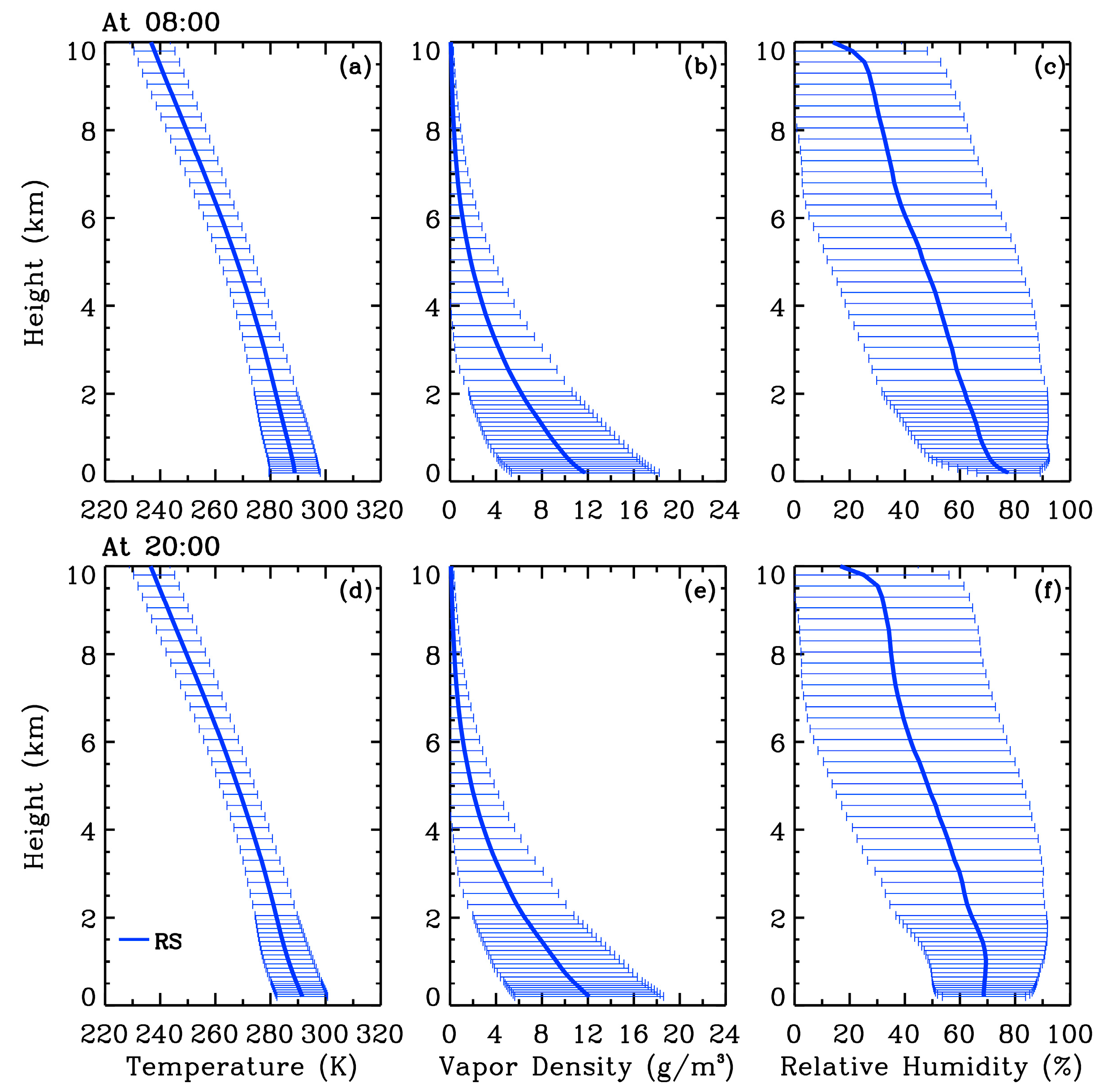
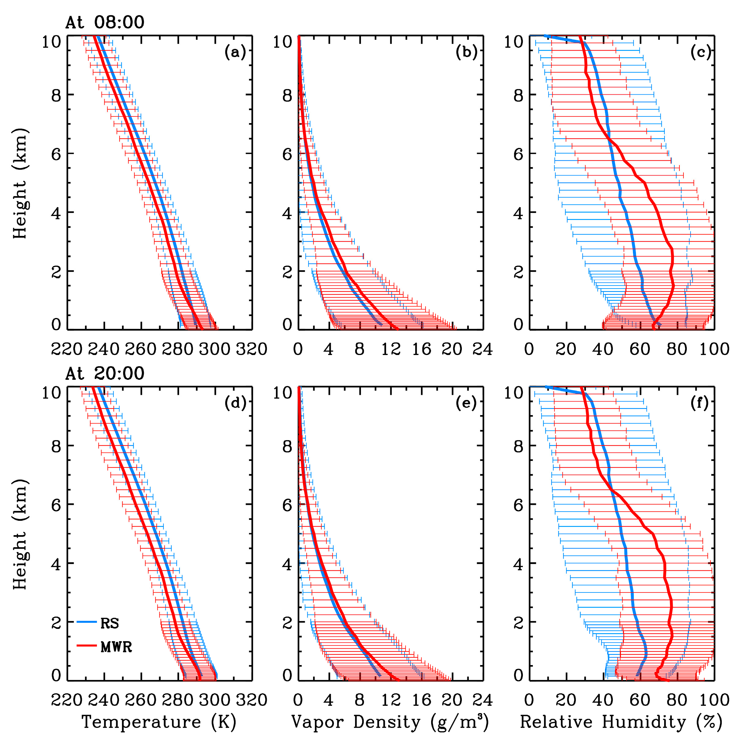
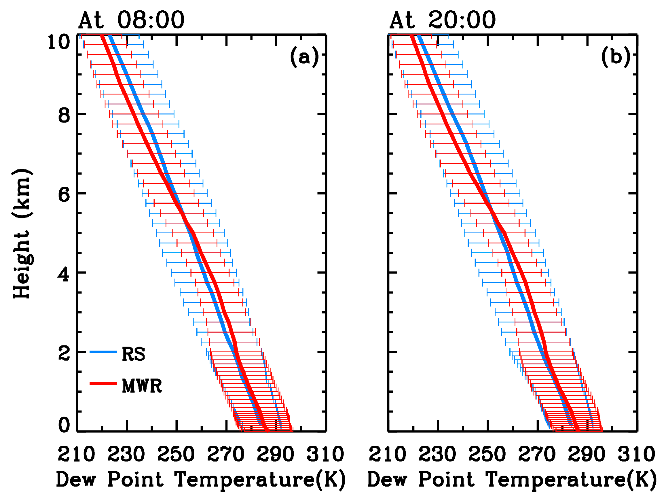
  • Based on the MWR and RS measurements at 8:00 and 20:00 LT, the differences between the mean temperature (and dew point temperature) derived from the MWR retrievals, and the mean temperature derived from RS observations in non-precipitation conditions are small below 2 km. Above 2 km, the MWR average temperature is about 1.8–2.8 and 2.5–3.5 K lower than the RS average temperature at 8:00 and 20:00, respectively. The difference of average water vapor densities is within 1.5 gm−3 near the ground and decreases with height. In general, compared with the relative humidity in the RS measurement, the relative humidity is higher in the MWR observation below 6.5 km, with the difference within 20%. In the seasonal averages, the temperature and water vapor content biases are roughly consistent with those in the 21-month averages, except for a larger water vapor bias near the ground in summer. The MWR and RS relative humidity data have correlation coefficients of 0.6–0.9 at different heights, and their bias is generally in the range of −15% to 20% but with different seasonal profiles. The results are roughly consistent with those in different sites from previous studies where the temperature is generally 0–3 K lower in the MWR data than in the RS data but the humidity is about 0–20% higher [31,32,67]. In addition, differences between the MWR and RS observations vary with height and season, which is similar to the differences recorded in in previous studies [64,65,68]. The discrepancy between the two measurements may be related to the sensing methods, retrieval algorithms, two-site distance, and environment around the MWR site.
  • We averaged the temperature, water vapor, and relative humidity during the precipitation and non-precipitation periods in the four seasons from the MWR observations, respectively. The mean surface temperature during precipitation periods is close to that during non-precipitation periods in winter and spring, but 4.2 and 6.8 K lower than that during non-precipitation periods in summer and autumn, respectively; as the Chinese proverb goes, “one autumn rain, one cold, and after ten autumn rains, you need to put on cotton clothes”. The mean vapor content near the ground is higher in precipitation than in non-precipitation conditions in spring, summer, and winter, whereas it is slightly lower in precipitation conditions in autumn due to the strong cooling that occurs in precipitation conditions. These results indicate that precipitation in Wuhan during autumn is mainly caused by cold air from the north. Under precipitation conditions, the relative humidity exceeds 90% from the ground to 5 km, especially to 6.5 km in summer, which is obviously larger relative to that under non-precipitation conditions. In early studies, the temperature and humidity from the MWR observations also show the different features between precipitation and non-precipitation events [69,70].
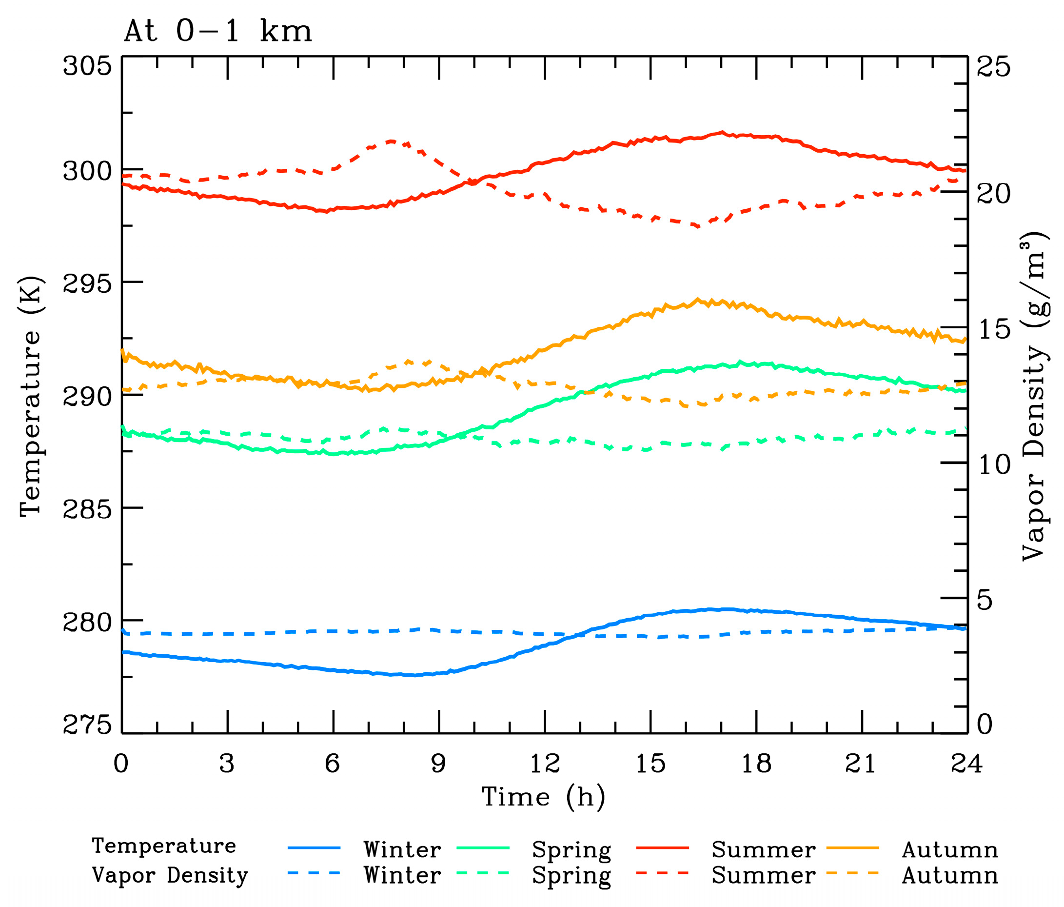
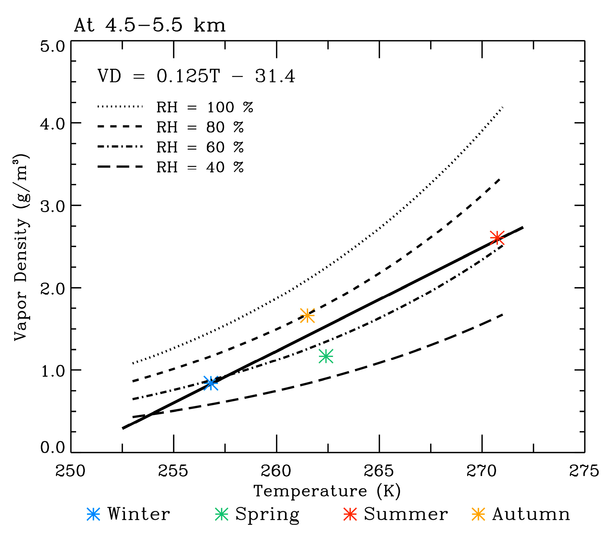
  • On the seasonal scale, the averaged water vapor density in the height range of 0–1.0 km during non-precipitation events shows an approximately linear increase with the average temperature, with the increment of about 0.78 gm−3 for the temperature rise of 1 K; nevertheless, as the altitude rises, their relationship gradually deviates from the linear form due to the effect of water vapor transport. In each season, the mean temperature at 0–1.0 km clearly displays a diurnal change with the maximum temperature at about 16:40–17:40 and the minimum temperature at 6:30–8:30. Because of the change of the boundary layer height due to radiation heating and cooling, the mean water vapor content has a diurnal variation opposite to the temperature, with the correlation coefficients of −0.69, −0.95, −0.93, and −0.56 in the range of 0–0.5 km from spring to winter. In the height ranges of 4.5–5.5 km and 8.5–9.5 km, the temperature shows a synchronized diurnal evolution, with correlation coefficients of 0.99, 0.97, and 0.97 from spring to autumn, and the maximum value prior to that at 0–1.0 km, for example, about 3 h earlier in summer. This indicates the strong influence of the air–land interaction on the temperature near the ground, but the weak influence on the free atmosphere above 4.5 km. The time when the maximum temperature occurs in summer is different from that in the Tibetan Plateau [47], which indicates that diurnal variations in the temperature differ regionally. In the two height ranges, the diurnal change of temperature is small in winter. In summer, the diurnal variation in the water vapor density at 8.5–9.5 km is opposite to that in the temperature, with a correlation coefficient of −0.85, similar to that at 0–1.0 km, while at 4.5–5.5 km, the water vapor content exhibits a positive correlation with the temperature from about 8:00 to 19:00, but an inverse correlation at other times. A similar scenario can be seen in spring and autumn, but with a weaker correlation.
This investigation is helpful for deepening our understanding of the temperature and humidity variabilities and their relationship over Wuhan. Meanwhile, since temperature and humidity are the important two input parameters for weather and climate models, the quantitative clarification of the seasonal and diurnal changes in temperature and water vapor is conducive for improving the reliability and accuracy of weather and climate model output results. With the aid of the MWR measurements with high temporal resolution, we will gain further insight into the dynamics and thermodynamics involved in various weather processes in the future.

Author Contributions

Conceptualization, K.H. and X.G.; methodology, K.H., X.G., and F.Y.; investigation, X.G. and R.C.; visualization, X.G. and Z.Z.; data curation, K.H., X.G., and J.F.; funding acquisition, K.H. All authors have read and agreed to the published version of the manuscript.

Funding

This work was supported by the National Key Research and Development Program of China (2022YFB3901800, and 2022YFB3901805) and the National Natural Science Foundation of China (41974176, and 42174189).

Data Availability Statement

The radiosonde data is accessible from http://weather.uwyo.edu/upperair/sounding.html (accessed on 12 November 2023)”.

Acknowledgments

We are grateful to the editor and anonymous reviewers for their valuable comments on our paper. We thank the University of Wyoming for providing the radiosonde data.

Conflicts of Interest

The authors declare no conflict of interest.

References

  1. Maher, P.; Gerber, E.P.; Medeiros, B.; Merlis, T.M.; Sherwood, S.; Sheshadri, A.; Sobel, A.H.; Vallis, G.K.; Voigt, A.; Zurita-Gotor, P. Model hierarchies for understanding atmospheric circulation. Rev. Geophys. 2019, 57, 250–280. [Google Scholar] [CrossRef]
  2. Ma, H.-Y.; Klein, S.A.; Xie, S.; Zhang, C.; Tang, S.; Tang, Q.; Morcrette, C.J.; Van Weverberg, K.; Petch, J.; Ahlgrimm, M.; et al. Causes: On the role of surface energy budget errors to the warm surface air temperature error over the central United States. J. Geophys. Res. Atmos. 2018, 123, 2888–2909. [Google Scholar] [CrossRef]
  3. Schneider, T.; O’Gorman, P.A.; Levine, X.J. Water vapor and the dynamics of climate changes. Rev. Geophys. 2010, 48, RG3001. [Google Scholar] [CrossRef]
  4. Sherwood, S.C.; Roca, R.; Weckwerth, T.M.; Andronova, N.G. Tropospheric water vapor, convection, and climate. Rev. Geophys. 2010, 48, RG2001. [Google Scholar] [CrossRef]
  5. Held, I.M.; Soden, B.J. Water vapor feedback and global warming. Annu. Rev. Energy Environ. 2000, 25, 441–475. [Google Scholar] [CrossRef]
  6. Rosenlof, K.H.; Reid, G.C. Trends in the temperature and water vapor content of the tropical lower stratosphere: Sea surface connection. J. Geophys. Res. Atmos. 2008, 113, 15. [Google Scholar] [CrossRef]
  7. Li, Z.H.; Li, Y.P.; Bonsal, B.; Manson, A.H.; Scaff, L. Combined impacts of ENSO and MJO on the 2015 growing season drought on the Canadian Prairies. Hydrol. Earth Syst. Sci. 2018, 22, 5057–5067. [Google Scholar] [CrossRef]
  8. Vaquero-Martínez, J.; Antón, M.; Sanchez-Lorenzo, A.; Cachorro, V.E. Evaluation of water vapor radiative effects using GPS data series over Southwestern Europe. Remote Sens. 2020, 12, 1307. [Google Scholar] [CrossRef]
  9. Stein, A.F.; Draxler, R.R.; Rolph, G.D.; Stunder, B.J.B.; Cohen, M.D.; Ngan, F. Noaa’s Hysplit atmospheric transport and dispersion modeling system. Bull. Am. Meteorol. Soc. 2015, 96, 2059–2077. [Google Scholar] [CrossRef]
  10. Sun, Y.L.; Yang, F.; Liu, M.J.; Li, Z.C.; Gong, X.; Wang, Y.Y. Evaluation of the weighted mean temperature over China using multiple reanalysis data and radiosonde. Atmos. Res. 2023, 285, 106664. [Google Scholar] [CrossRef]
  11. Pratt, R.W. Review of radiosonde humidity and temperature errors. J. Atmos. Ocean. Technol. 1985, 2, 404–407. [Google Scholar] [CrossRef]
  12. Wang, J.H.; Zhang, L.Y.; Dai, A.G.; Immler, F.; Sommer, M.; Vomel, H. Radiation dry bias correction of Vaisala RS92 humidity data and its impacts on historical radiosonde data. J. Atmos. Ocean. Technol. 2013, 30, 197–214. [Google Scholar] [CrossRef]
  13. Comiso, J.C. Arctic warming signals from satellite observations. Weather 2006, 61, 70–76. [Google Scholar] [CrossRef]
  14. Liang, C.K.; Eldering, A.; Gettelman, A.; Tian, B.; Wong, S.; Fetzer, E.J.; Liou, K.N. Record of tropical interannual variability of temperature and water vapor from a combined AIRS-MLS data set. J. Geophys. Res. Atmos. 2011, 116, 14841. [Google Scholar] [CrossRef]
  15. Garfinkel, C.I.; Waugh, D.W.; Oman, L.D.; Wang, L.; Hurwitz, M.M. Temperature trends in the tropical upper troposphere and lower stratosphere: Connections with sea surface temperatures and implications for water vapor and ozone. J. Geophys. Res. Atmos. 2013, 118, 9658–9672. [Google Scholar] [CrossRef]
  16. Wang, J.H.; Hock, T.; Cohn, S.A.; Martin, C.; Potts, N.; Reale, T.; Sun, B.M.; Tilley, F. Unprecedented upper-air dropsonde observations over Antarctica from the 2010 Concordiasi Experiment: Validation of satellite-retrieved temperature profiles. Geophys. Res. Lett. 2013, 40, 1231–1236. [Google Scholar] [CrossRef]
  17. Wong, S.; Fetzer, E.J.; Schreier, M.; Manipon, G.; Fishbein, E.F.; Kahn, B.H.; Yue, Q.; Irion, F.W. Cloud-induced uncertainties in AIRS and ECMWF temperature and specific humidity. J. Geophys. Res. Atmos. 2015, 120, 1880–1901. [Google Scholar] [CrossRef]
  18. Bedoya-Velásquez, A.E.; Herreras-Giralda, M.; Román, R.; Wiegner, M.; Lefebvre, S.; Toledano, C.; Huet, T.; Ceolato, R. Ceilometer inversion method using water-vapor correction from co-located microwave radiometer for aerosol retrievals. Atmos. Res. 2021, 250, 105379. [Google Scholar] [CrossRef]
  19. Kim, D.K.; Lee, D.I. Atmospheric thickness and vertical structure properties in wintertime precipitation events from microwave radiometer, radiosonde and wind profiler observations. Meteorol. Appl. 2015, 22, 599–609. [Google Scholar] [CrossRef]
  20. Harikishan, G.; Padmakumari, B.; Maheskumar, R.S.; Pandithurai, G.; Min, Q.L. Macrophysical and microphysical properties of monsoon clouds over a rain shadow region in India from ground- based radiometric measurements. J. Geophys. Res. Atmos. 2014, 119, 4736–4749. [Google Scholar] [CrossRef]
  21. Zhao, Y.X.; Yan, H.L.; Wu, P.; Zhou, D. Linear correction method for improved atmospheric vertical profile retrieval based on ground-based microwave radiometer. Atmos. Res. 2020, 232, 104678. [Google Scholar] [CrossRef]
  22. Rambabu, S.; Pillai, J.S.; Agarwal, A.; Pandithurai, G. Evaluation of brightness temperature from a forward model of ground-based microwave radiometer. J. Earth Syst. Sci. 2014, 123, 641–650. [Google Scholar] [CrossRef]
  23. Del Frate, F.; Schiavon, G. A combined natural orthogonal functions neural network technique for the radiometric estimation of atmospheric profiles. Radio Sci. 1998, 33, 405–410. [Google Scholar] [CrossRef]
  24. Churnside, J.H.; Stermitz, T.A.; Schroeder, J.A. Temperature profiling with neural network inversion of microwave radiometer data. J. Atmos. Ocean. Technol. 1994, 11, 105–109. [Google Scholar] [CrossRef]
  25. Del Frate, F.; Schiavon, G. A neural network algorithm for the retrieval of atmospheric profiles from radiometric data. In Proceedings of the 1997 IEEE International Geoscience and Remote Sensing Symposium Proceedings. Remote Sensing—A Scientific Vision for Sustainable Development, Singapore, 3–8 August 1997; pp. 2097–2099. [Google Scholar] [CrossRef]
  26. Ying, H.J.; Wei, Z.S.; Yu, Z.A. The primary design of advanced ground-based atmospheric microwave sounder and retrieval of physical parameters. J. Quant. Spectrosc. Radiat. Transf. 2011, 112, 236–246. [Google Scholar] [CrossRef]
  27. Ratnam, M.V.; Santhi, Y.D.; Rajeevan, M.; Rao, S.V.B. Diurnal variability of stability indices observed using radiosonde observations over a tropical station: Comparison with microwave radiometer measurements. Atmos. Res. 2013, 124, 21–33. [Google Scholar] [CrossRef]
  28. Chan, W.S.; Lee, J.C.W. Vertical profile retrievals with warm-rain microphysics using the ground-based microwave radiometer operated by the Hong Kong Observatory. Atmos. Res. 2015, 161, 125–133. [Google Scholar] [CrossRef]
  29. Xu, G.R.; Xi, B.K.; Zhang, W.G.; Cui, C.G.; Dong, X.Q.; Liu, Y.Y.; Yan, G.P. Comparison of atmospheric profiles between microwave radiometer retrievals and radiosonde soundings. J. Geophys. Res. Atmos. 2015, 120, 10313–10323. [Google Scholar] [CrossRef]
  30. Xu, G.R.; Ware, R.; Zhang, W.G.; Feng, G.L.; Liao, K.W.; Liu, Y.B. Effect of off-zenith observations on reducing the impact of precipitation on ground-based microwave radiometer measurement accuracy. Atmos. Res. 2014, 140, 85–94. [Google Scholar] [CrossRef]
  31. Chan, P.W. Performance and application of a multi-wavelength, ground-based microwave radiometer in intense convective weather. Meteorol. Z. 2009, 18, 253–265. [Google Scholar] [CrossRef]
  32. Temimi, M.; Fonseca, R.M.; Nelli, N.R.; Valappil, V.K.; Weston, M.J.; Thota, M.S.; Wehbe, Y.; Yousef, L. On the analysis of ground-based microwave radiometer data during fog conditions. Atmos. Res. 2020, 231, 104652. [Google Scholar] [CrossRef]
  33. Rose, T.; Crewell, S.; Lohnert, U.; Simmer, C. A network suitable microwave radiometer for operational monitoring of the cloudy atmosphere. Atmos. Res. 2005, 75, 183–200. [Google Scholar] [CrossRef]
  34. Massaro, G.; Stiperski, I.; Pospichal, B.; Rotach, M.W. Accuracy of retrieving temperature and humidity profiles by ground-based microwave radiometry in truly complex terrain. Atmos. Meas. Tech. 2015, 8, 3355–3367. [Google Scholar] [CrossRef]
  35. Bernet, L.; Navas-Guzman, F.; Kampfer, N. The effect of cloud liquid water on tropospheric temperature retrievals from microwave measurements. Atmos. Meas. Tech. 2017, 10, 4421–4437. [Google Scholar] [CrossRef]
  36. Zhang, W.G.; Xu, G.R.; Liu, Y.Y.; Yan, G.P.; Li, D.J.; Wang, S.B. Uncertainties of ground-based microwave radiometer retrievals in zenith and off-zenith observations under snow conditions. Atmos. Meas. Tech. 2017, 10, 155–165. [Google Scholar] [CrossRef]
  37. Knupp, K.R.; Ware, R.; Cimini, D.; Vandenberghe, F.; Vivekanandan, J.; Westwater, E.; Coleman, T.; Phillips, D. Ground-based passive microwave profiling during dynamic weather conditions. J. Atmos. Ocean. Technol. 2009, 26, 1057–1073. [Google Scholar] [CrossRef]
  38. Marzano, F.S.; Cimini, D.; Ware, R.H. Monitoring of rainfall by ground-based passive microwave systems: Models, measurements and applications. Adv. Geosci. 2005, 2, 259–265. [Google Scholar] [CrossRef]
  39. Coen, M.C.; Praz, C.; Haefele, A.; Ruffieux, D.; Kaufmann, P.; Calpini, B. Determination and climatology of the planetary boundary layer height above the Swiss plateau by in situ and remote sensing measurements as well as by the COSMO-2 model. Atmos. Chem. Phys. 2014, 14, 13205–13221. [Google Scholar] [CrossRef]
  40. Moreira, G.D.; Guerrero-Rascado, J.L.; Bravo-Aranda, J.A.; Benavent-Oltra, J.A.; Ortiz-Amezcua, P.; Roman, R.; Bedoya-Velasquez, A.E.; Landulfo, E.; Alados-Arboledas, L. Study of the planetary boundary layer by microwave radiometer, elastic lidar and Doppler lidar estimations in Southern Iberian Peninsula. Atmos. Res. 2018, 213, 185–195. [Google Scholar] [CrossRef]
  41. Jiang, Y.Y.; Xin, J.Y.; Zhao, D.D.; Jia, D.J.; Tang, G.Q.; Quan, J.N.; Wang, M.; Dai, L.D. Analysis of differences between thermodynamic and material boundary layer structure: Comparison of detection by ceilometer and microwave radiometer. Atmos. Res. 2021, 248, 105179. [Google Scholar] [CrossRef]
  42. Hansen, J.; Sato, M.; Ruedy, R. Perception of climate change. Proc. Natl. Acad. Sci. USA 2012, 109, E2415–E2423. [Google Scholar] [CrossRef] [PubMed]
  43. Korhonen, K.; Giannakaki, E.; Mielonen, T.; Pfuller, A.; Laakso, L.; Vakkari, V.; Baars, H.; Engelmann, R.; Beukes, P.; Van Zyl, P.G.; et al. Atmospheric boundary layer top height in South Africa: Measurements with lidar and radiosonde compared to three atmospheric models. Atmos. Chem. Phys. 2014, 14, 4263–4278. [Google Scholar] [CrossRef]
  44. Li, Z.Q.; Lau, W.K.M.; Ramanathan, V.; Wu, G.; Ding, Y.; Manoj, M.G.; Liu, J.; Qian, Y.; Li, J.; Zhou, T.; et al. Aerosol and monsoon climate interactions over Asia. Rev. Geophys. 2016, 54, 866–929. [Google Scholar] [CrossRef]
  45. Moreira, G.D.; Guerrero-Rascado, J.L.; Bravo-Aranda, J.A.; Foyo-Moreno, I.; Cazorla, A.; Alados, I.; Lyamani, H.; Landulfo, E.; Alados-Arboledas, L. Study of the planetary boundary layer height in an urban environment using a combination of microwave radiometer and ceilometer. Atmos. Res. 2020, 240, 104932. [Google Scholar] [CrossRef]
  46. Seidel, D.J.; Ao, C.O.; Li, K. Estimating climatological planetary boundary layer heights from radiosonde observations: Comparison of methods and uncertainty analysis. J. Geophys. Res. Atmos. 2010, 115, D16113. [Google Scholar] [CrossRef]
  47. Sun, N.; Zhong, L.; Zhao, C.; Ma, M.; Fu, Y.F. Temperature, water vapor and tropopause characteristics over the Tibetan Plateau in summer based on the COSMIC, ERA-5 and IGRA datasets. Atmos. Res. 2022, 266, 105955. [Google Scholar] [CrossRef]
  48. Liu, G.R.; Liu, C.C.; Kuo, T.H. Rainfall intensity estimation by ground-based dual-frequency microwave radiometers. J. Appl. Meteorol. Clim. 2001, 40, 1035–1041. [Google Scholar] [CrossRef]
  49. Zhang, W.G.; Xu, G.R.; Xi, B.K.; Ren, J.; Wan, X.; Zhou, L.L.; Cui, C.G.; Wu, D.Q. Comparative study of cloud liquid water and rain liquid water obtained from microwave radiometer and micro rain radar observations over central China during the monsoon. J. Geophys. Res. Atmos. 2020, 125, e2020JD032456. [Google Scholar] [CrossRef]
  50. Chan, P.W.; Hon, K.K. Application of ground-based, multi-channel microwave radiometer in the nowcasting of intense convective weather through instability indices of the atmosphere. Meteorol. Z. 2011, 20, 431–440. [Google Scholar] [CrossRef]
  51. Cui, C.G.; Wan, R.; Wang, B.; Dong, X.Q.; Li, H.L.; Wang, X.K.; Xu, G.R.; Wang, X.F.; Wang, Y.H.; Xiao, Y.J.; et al. The Mesoscale Heavy Rainfall Observing System (MHROS) over the middle region of the Yangtze River in China. J. Geophys. Res. Atmos. 2015, 120, 10399–10417. [Google Scholar] [CrossRef]
  52. Ming, H.; Wei, M.; Wang, M.Z.; Gao, L.H.; Chen, L.J.; Wang, X.C. Analysis of fog at Xianyang Airport based on multi-source ground-based detection data. Atmos. Res. 2019, 220, 34–45. [Google Scholar] [CrossRef]
  53. Tian, M.; Wu, B.G.; Huang, H.; Zhang, H.S.; Zhang, W.Y.; Wang, Z.Y. Impact of water vapor transfer on a Circum-Bohai-Sea heavy fog: Observation and numerical simulation. Atmos. Res. 2019, 229, 1–22. [Google Scholar] [CrossRef]
  54. Turner, D.D.; Goldsmith, J.E.M. Twenty-four-hour Raman lidar water vapor measurements during the Atmospheric radiation Measurement program’s 1996 and 1997 water vapor intensive observation periods. J. Atmos. Ocean. Technol. 1999, 16, 1062–1076. [Google Scholar] [CrossRef]
  55. Mattis, I.; Ansmann, A.; Althausen, D.; Jaenisch, V.; Wandinger, U.; Muller, D.; Arshinov, Y.F.; Bobrovnikov, S.M.; Serikov, I.B. Relative-humidity profiling in the troposphere with a Raman lidar. Appl. Opt. 2002, 41, 6451–6462. [Google Scholar] [CrossRef]
  56. Ware, R.; Carpenter, R.; Guldner, J.; Liljegren, J.; Nehrkorn, T.; Solheim, F.; Vandenberghe, F. A multichannel radiometric profiler of temperature, humidity, and cloud liquid. Radio Sci. 2003, 38, 8079. [Google Scholar] [CrossRef]
  57. Jin, S.K.; Ma, Y.Y.; Zhang, M.; Gong, W.; Lei, L.F.; Ma, X. Comparation of aerosol optical properties and associated radiative effects of air pollution events between summer and winter: A case study in January and July 2014 over Wuhan, Central China. Atmos. Environ. 2019, 218, 117004. [Google Scholar] [CrossRef]
  58. Bedoya-Velásquez, A.E.; Navas-Guzmán, F.; Moreira, G.D.; Román, R.; Cazorla, A.; Ortiz-Amezcua, P.; Benavent-Oltra, J.A.; Alados-Arboledas, L.; Olmo-Reyes, F.J.; Foyo-Moreno, I.; et al. Seasonal analysis of the atmosphere during five years by using microwave radiometry over a mid-latitude site. Atmos. Res. 2019, 218, 78–89. [Google Scholar] [CrossRef]
  59. Madhulatha, A.; Rajeevan, M.; Ratnam, M.V.; Bhate, J.; Naidu, C.V. Nowcasting severe convective activity over southeast India using ground-based microwave radiometer observations. J. Geophys. Res. Atmos. 2013, 118, 1–13. [Google Scholar] [CrossRef]
  60. Cady-Pereira, K.E.; Shephard, M.W.; Turner, D.D.; Mlawer, E.J.; Clough, S.A.; Wagner, T.J. Improved daytime column-integrated precipitable water vapor from Vaisala radiosonde humidity sensors. J. Atmos. Ocean. Technol. 2008, 25, 873–883. [Google Scholar] [CrossRef]
  61. Westwater, E.R.; Stankov, B.B.; Cimini, D.; Han, Y.; Shaw, J.A.; Lesht, B.M.; Long, C.N. Radiosonde humidity soundings and microwave radiometers during Nauru99. J. Atmos. Ocean. Technol. 2003, 20, 953–971. [Google Scholar] [CrossRef]
  62. Turner, D.D.; Lesht, B.M.; Clough, S.A.; Liljegren, J.C.; Revercomb, H.E.; Tobin, D.C. Dry bias and variability in Vaisala RS80-H radiosondes: The ARM experience. J. Atmos. Ocean. Technol. 2003, 20, 117–132. [Google Scholar] [CrossRef]
  63. Çengel, Y.A.; Boles, M.A. Thermodynamics: An Engineering Approach, 3rd ed.; McGraw-Hill: Boston, MA, USA, 1989; ISBN 0-07-011927-9. [Google Scholar]
  64. Liu, M.; Liu, Y.A.; Shu, J. Characteristics analysis of the multi-channel ground-based microwave radiometer observations during various weather conditions. Atmosphere 2022, 13, 1556. [Google Scholar] [CrossRef]
  65. Liu, H.Y. The temperature profile comparison between the ground-based microwave radiometer and the other instrument for the recent three years. Acta Meteorol. Sin. 2011, 4, 719–728. [Google Scholar] [CrossRef]
  66. Drobinski, P.; Alonzo, B.; Bastin, S.; Silva, N.D.; Muller, C. Scaling of precipitation extremes with temperature in the French Mediterranean region: What explains the hook shape? J. Geophys. Res. Atmos. 2016, 121, 3100–3119. [Google Scholar] [CrossRef]
  67. Shrestha, B.; Brotzge, J.A.; Wang, J.H. Evaluation of the New York State Mesonet Profiler Network data. Atmos. Meas. Tech. 2022, 15, 6011–6033. [Google Scholar] [CrossRef]
  68. Renju, R.; Raju, C.S.; Swathi, R.; Milan, V.G. Retrieval of atmospheric temperature and humidity profiles over a tropical coastal station from ground-based Microwave Radiometer using deep learning technique. J. Atmos. Sol. Terr. Phys. 2023, 249, 106094. [Google Scholar] [CrossRef]
  69. Ma, R.J.; Li, X.F. Sounding data from ground-based microwave radiometers for a hailstorm case: Analyzing spatiotemporal differences and initializing an idealized model for prediction. Atmosphere 2022, 13, 1535. [Google Scholar] [CrossRef]
  70. Qi, Y.J.; Fan, S.Y.; Li, B.; Mao, J.J.; Lin, D.W. Assimilation of ground-based microwave radiometer on heavy rainfall forecast in Beijing. Atmosphere 2022, 13, 74. [Google Scholar] [CrossRef]
Figure 1. Topographic map of Hubei and microwave radiometer site in Wuhan University.
Remotesensing 15 05422 g001
Figure 2. Mean values and standard deviations of (a,d) temperature, (b,e) vapor density, and (c,f) relative humidity at (ac) 8:00 and (df) 20:00 in Wuhan from 2015 to 2019 used to train the neural network.
Remotesensing 15 05422 g002
Figure 3. Mean values and standard deviations of (a,d) temperature, (b,e) vapor density, (c,f) relative humidity observed with (red) MWR and (blue) RS at (ac) 8:00 and (df) 20:00 during non-precipitation events throughout 21 months.
Remotesensing 15 05422 g003
Figure 4. Mean values and standard deviations of dew point temperature from (red) MWR and (blue) RS data at (a) 8:00 and (b) 20:00 during non-precipitation events throughout 21 months.
Remotesensing 15 05422 g004
Figure 5. (ac) Correlation coefficients and (df) biases of (a,d) temperature, (b,e) water vapor density, and (c,f) relative humidity between MWR and RS observations at 8:00 and 20:00 during non-precipitation events throughout 21 months. The green, red, orange, and blue lines represent the results in spring, summer, autumn and winter, respectively.
Remotesensing 15 05422 g005
Figure 6. Emagram of MWR and radiosonde data in conditions of (a) rain at 20:00 on 1 July 2021 and (b) snow at 8:00 on 29 December 2020. The thick red lines correspond to the MWR (right) temperature and (left) dew point temperature, and the thick blue lines correspond to the radiosonde (right) temperature and (left) dew point temperature.
Remotesensing 15 05422 g006
Figure 7. Profiles of seasonally averaged (a) temperature, (b) water vapor density, and (c) relative humidity in precipitation and non-precipitation conditions. The green, red, orange, and blue lines represent the results from spring to winter, and the solid and dashed curves denote the results under the conditions of precipitation and non-precipitation, respectively.
Remotesensing 15 05422 g007
Figure 8. Diurnal variations of (ad) temperature and (eh) water vapor density under non-precipitation conditions in (a,e) winter, (b,f) spring, (c,g) summer, and (d,h) autumn from MWR observation throughout 21 months.
Remotesensing 15 05422 g008
Figure 9. Diurnal variations of temperature and water vapor density averaged within 1 km under non-precipitation conditions in four seasons. The solid line denotes the temperature scaled on the left axis, and the dashed line denotes the water vapor density scaled on the right axis. The green, red, orange, and blue lines represent the results from spring to winter, respectively.
Remotesensing 15 05422 g009
Figure 10. Diurnal variations of temperature and water vapor density averaged (a) from 8.5 to 9.5 km and (b) 4.5 to 5.5 km under non-precipitation conditions in four seasons. The solid line denotes the temperature scaled on the left axis, and the dashed line denotes the water vapor density scaled on the right axis. The green, red, orange, and blue lines represent the results in spring, summer, autumn and winter, respectively.
Remotesensing 15 05422 g010
Figure 11. Temperature and water vapor density averaged within 1 km under non-precipitation conditions in four seasons and (solid black line) their linear fit, and relationship between water vapor and temperature at relative humidities of (dotted curve) 100%, (short dash curve) 80%, (dash-dotted curve) 60%, and (long dash curve) 40% derived from Clausius–Clapeyron Equation. The green, red, orange, and blue asterisks denote the values in spring, summer, autumn, and winter, respectively.
Remotesensing 15 05422 g011
Figure 12. Temperature and water vapor density averaged at 4.5–5.5 km under non-precipitation conditions in four seasons and (solid black line) their linear fit, and relationship between water vapor and temperature at relative humidities of (dotted curve) 100%, (short dash curve) 80%, (dash-dotted curve) 60%, and (long dash curve) 40% derived from Clausius–Clapeyron Equation. The green, red, orange, and blue asterisks denote the values in spring, summer, autumn, and winter, respectively.
Remotesensing 15 05422 g012
Disclaimer/Publisher’s Note: The statements, opinions and data contained in all publications are solely those of the individual author(s) and contributor(s) and not of MDPI and/or the editor(s). MDPI and/or the editor(s) disclaim responsibility for any injury to people or property resulting from any ideas, methods, instructions or products referred to in the content.

