Abstract
In soybean, lodging is sometimes caused by strong winds and rains, resulting in a decrease in yield and quality. Technical measures against lodging include “pinching”, in which the main stem is pruned when excessive growth is expected. However, there can be a decrease in yield when pinching is undertaken when the risk of lodging is relatively low. Therefore, it is important that pinching is performed after the future risk of lodging has been determined. The lodging angle at the full maturity stage (R8) can be explained using a multiple regression model with main stem elongation from the sixth leaf stage (V6) to the blooming stage (R1) and main stem length at the full seed stage (R6) as the explanatory variables. The objective of this study was to develop an areal lodging prediction method by combining a main stem elongation model with areal main stem length estimation using UAV remote sensing. The main stem elongation model from emergence to R1 was a logistic regression formula with the temperature and daylight hours functions f (Ti, Di) as the explanatory variables. The main stem elongation model from R1 to the peak main stem length was a linear regression formula with the main stem length of R1 as the explanatory variable. The model that synthesized these two regression formulas were used as the main stem elongation model from emergence to R8. The accuracy of the main stem elongation model was tested on the test data, and the average RMSE was 5.3. For the areal main stem length estimation by UAV remote sensing, we proposed a soil-adjusted vegetation index (SAVIvc) that takes vegetation cover into account. SAVIvc was more accurate in estimating the main stem length than the previously reported vegetation index (R2 = 0.78, p < 0.001). The main stem length estimated by the main stem elongation model combined with SAVIvc was substituted into a multiple regression model of lodging angle to test the accuracy of the areal lodging prediction method. The method was able to predict lodging angles with an accuracy of RMSE = 8.8. These results suggest that the risk of lodging can be estimated in an areal manner prior to pinching, even though the actual occurrence is affected by wind.
1. Introduction
Lodging of soybean is one of the meteorological disasters. Excess growth of soybean often increases the risk of lodging, but it occurs at strong winds and rains. Soybean yields can be reduced by 9–34% due to lodging [1]. Uchikawa et al. reported that when the combine harvester’s cutting height is lowered to reduce harvest losses due to lodging, soil scraping causes contamination of grains [2]. Given that lodging causes yield loss and quality deterioration, measures such as the introduction of lodging-resistant varieties have been taken. One technical measure is pinching, which involves pruning the main stem when excessive growth is expected [3]. Pinching is an effective measure when native varieties are in high demand in Japan, where soybean eating culture is deeply rooted, and a switch to lodging-resistant varieties cannot be achieved. However, if there is no difference in the degree of lodging between the no-pinching and pinching areas, the yield of the pinching area can be lower [4]. Therefore, it is important to implement pinching based on the prediction of future lodging.
Lodging is affected by the main stem length together with wind speed [5,6]. Konno and Homma reported that main stem elongation, especially from the 6th leaf stage to the blooming stage, and the main stem length after the blooming stage have an effect on lodging [6]. If the amount of main stem elongation and the main stem length during this period could be predicted before pinching, countermeasures could be taken to address the risk of lodging. Nakano et al. reported a model for predicting the number of main stem nodes for predicting main stem growth [7]. The model showed that the rate of increase in the main stem node number (node day−1) depends on the temperature. The main stem length is closely related to the number of main stem nodes [8,9]. It is likely that the main stem length can also be predicted as a function of temperature. Furthermore, the main stem length is also affected by the light environment and is higher under shading conditions and with relatively low daylight hours [10,11,12]. Therefore, the prediction of the main stem length should also take daylight into account. However, to date, there have been no studies on main stem elongation models, and there are no methods for predicting lodging through the prediction of main stem elongation that has yet been established.
Soybean growth differences are affected by soil physicochemical properties [13]. Differences in soil physicochemical properties have been found, including within the same field [14]. Yamamoto et al. investigated soybean SPAD values (an index of relative chlorophyll content; the name comes from the Soil and Plant Analyzer Development project [15]; the values measured with Konica Minolta’s SPAD-502 plus, Konica Minolta Japan, Inc., Tokyo, Japan) at 80 locations within a 5-ha farmer’s field and reported within-field differences [16]. This suggests that it is difficult to predict lodging at the field scale only using a growth model. Therefore, remote sensing is expected to be used as a diagnostic method for areal field growth. Yamamoto et al. conducted UAV remote sensing simultaneously with leaf color value research and found a significant relationship between leaf color values and GNDVI (Green Normalized Difference Vegetation Index) [16,17]. Tambo et al. also highlighted the potential of using GNDVI to estimate the nitrogen content and above-ground dry matter weight of soybean [18].
However, Kamaki et al. found that a single regression using the NDVI (Normalized Difference Vegetation Index) could not be used to estimate the above-ground dry matter weight with sufficient accuracy [19]. They attributed this to the effect of reflections from the soil surface. If the amount of growth in the early stages of growth can be estimated when the inter-row spaces are exposed, as in this study, it is important to use a vegetation index that suppresses the influence of reflections from the soil surface. SAVI (Soil-Adjusted Vegetation Index) and MSAVI (Modified Soil-Adjusted Vegetation Index) have been developed as vegetation indices that consider the effect of soil [20,21]. These vegetation indices incorporate a soil adjustment term (L) into the equation to reduce the influence of reflections from the soil surface. The soil adjustment term (L) is calculated as a constant of 0.50. However, the soil adjustment term (L) is inversely related to the vegetation cover, and the soil adjustment term (L) should be adjusted according to the vegetation cover [20]. However, to date, a soil-adjusted vegetation index that takes the vegetation cover into account has not yet been reported. Furthermore, previous studies on soybean growth and the vegetation index have predominantly focused on the above-ground dry matter weight and nitrogen content, and none of them have shown a relationship with the main stem length, which is the measurement target of this study.
Therefore, the following analyses were conducted in this study to establish an areal lodging prediction method.
- Creation of a main stem elongation model using the main stem node number model of Nakano et al. [7]
- Creation of an areal main stem length estimation method using a soil-adjusted vegetation index that takes vegetation cover into account using UAV remote sensing
- Creation of an areal lodging prediction method by combining the main stem elongation model and the soil-adjusted vegetation index
The accuracy of the developed areal lodging prediction method was verified using test data.
2. Materials and Methods
The soybean cultivar ‘Miyagishirome’ was used in this study. ‘Miyagishirome’ was bred in the Miyagi Prefecture in 1961 through pure line selection from native varieties, and it is characterized by its large grain size and excellent quality of appearance. However, it is prone to lodging [22,23]. This is the main variety that is grown in 44% of the fields in Miyagi Prefecture.
2.1. Main Stem Elongation Modeling
2.1.1. Main Stem Elongation Model from Emergence Date to Blooming Stage (R1)
The main stem elongation model from emergence date to blooming stage (R1) ([24], and similarly for subsequent reproductive growth stages) used the temperature function f (Ti) (1) in the main stem node number model by Nakano et al. [7]. Given that the main stem length is affected by daylight hours, a temperature and daylight hours function f (Ti, Di) (2) was created by adding a daylight hours term to function (1). The term including daylight hours (Di) was set to 1 < {1 + exp (−a × Di)} < 2. This means that the maximum daily main stem growth (cm day−1) doubles when daylight hours are low. A logistic regression (3) with the daily accumulated value of this function (2) as the explanatory variable was used as the main stem elongation model.
Ti and Di in functions (1) and (2), and the main stem elongation model (3) denote mean daily temperature (°C) and daylight hours (h day−1), respectively. TNb, TNp1, TNp2, and TNc in function (1) indicate the lower, optimum, upper, and upper-temperature limits of the main stem node increase; 10.0 °C, 30.0 °C, 35.0 °C, and 45.0 °C were used for TNb, TNp1, TNp2, and TNc based on Nakano et al. [7]. MSLDAE in the main stem elongation model (3) represents the main stem length at days after emergence (DAE). a1, a2, b, and c in function (2), and the main stem elongation model (3) are parameters. a1 is the coefficient of daylight hours (Di). a2, b, and c are the rate of increase of main stem length, inflection point, and asymptote line.
The data used to create the model were the “main stem length” up to three days after the blooming stage, the average daily temperature (°C), and daylight hours (h day−1) from the 2005 to 2021 cropping pattern analysis test reported by Organization Miyagi Prefectural Furukawa Agricultural Experiment Station (n = 36, n indicates the number of data.) (Table 1) [25,26,27,28,29,30,31,32,33,34,35,36,37,38,39,40,41]. The emergence date, which is the starting point of the model, was also obtained from the crop analysis test. Meteorological data were obtained from the nearest AMeDAS (Japan Meteorological Agency) in the study area [42]. Parameters were obtained using a solver in Microsoft Excel 2019 (Microsoft) to minimize the RMSE between the estimated and measured main stem length.

Table 1.
Statistics from data used to create the main stem elongation model from emergence date to R1.
2.1.2. Main Stem Elongation Model from Blooming Stage (R1) to Peak Main Stem Length
The model predicted the peak main stem length from the main stem length at R1. The peak main stem length was reported by Konno and Homma to be at the beginning pod stage (R3) [6]. The main stem length remained flat from R3 to the full maturity stage (R8). Therefore, a model of peak main stem length was created using a single regression analysis with the main stem length at R1 as the explanatory variable and the main stem length after R3 as the objective variable. The main stem length was assumed to have a length that remained constant after the peak.
The data used to create the model were the main stem length data (n = 5) from the 60- and 80-day post-sowing research in the same cropping pattern analysis test as in (1) for the years when the difference in days between the research date and the R1 calendar date ranged from −1 to 5 days. The following main stem elongation model (4) was created assuming that this data was the R1 data and the 100 days after sowing research data was the peak main stem length data. Microsoft Excel 2019 and JMP14 (SAS Institute, Tokyo, Japan) were used to create the regression equations.
In the main stem elongation model (4), MSLpeak indicates the peak main stem length, MSLR1 indicates the main stem length of R1, and a3 and b2 are parameters. The main stem elongation models (3) and (4) were synthesized to obtain a main stem elongation model that can be adapted from post-emergence to R8.
2.1.3. Accuracy Verification of the Main Stem Elongation Model
The accuracy of the main stem elongation model was verified using main stem length data obtained in Osaki City and Kurihara City, Miyagi Prefecture, in 2022. Research plots were selected by visual inspection at moderate-growth sites (1.5 m−2), and research was conducted on moderate-growth individuals sampled from the vicinity of the experimental plots. Data for Osaki City was the average of two fields. Eight individuals were researched at the 4th leaf stage (V4), 6th leaf stage (V6), 8th leaf stage (V8), R1, R3, and full seed stage (R6) in Osaki City. In Kurihara City, eight to 12 individuals per field were researched at V4, the 7th leaf stage (V7), R1, R3, and R6. The main stem length was defined as the length from the beginning of the cotyledon to the highest node.
Sowing dates, emergence dates, and blooming stages (R1) were 25 May and 6 July (sowing dates), 15 June and 16 July (emergence dates), 1 August and 18 August (R1) in Osaki City, and 23 June (sowing date), 30 June (emergence date), and 9 August (R1) in Kurihara City.
2.2. Leaf Age Modeling
In line with the main stem elongation model (3), a leaf age model (5) was created using the temperature function f (Ti) (1) of the main stem node number model by Nakano et al. [7].
The main stem node number model of Nakano et al. is an accumulated value of a × f(Ti) [7]. In this study, leaf age was defined as the value obtained by subtracting 2.5 from the logistic regression applying the main stem node number model of Nakano et al. (2019) [7]. Assuming that the nth leaf develops during the extraction of the n + 1st node, leaf age (LN) was determined by subtracting 2.5, which was the number of the cotyledon node, primary leaf node, and the n + 1st node during extraction. In the leaf age model (5), a4, b3, and c2 are parameters indicating the rate of increase in the number of main stem nodes, inflection point, and asymptote line, respectively.
The data used to create the leaf age model (5) were the results of the cropping pattern analysis test from 2005 to 2021 (n = 53) (Table 2), as well as the data used to create the main stem elongation model (3) [25,26,27,28,29,30,31,32,33,34,35,36,37,38,39,40,41]. The leaf age model (5) used data at 40, 60, and 80 days after sowing. JMP14 was used to calculate the parameters.
Table 2.
Statistics from data used to create the leaf age model.
The leaf age model (5) was tested using the data obtained by the same research as in Section 2.1.3 in 2022 and the data sowing on 25 May and 24 June 2021 in Osaki City, in which only leaf age was studied (n = 21). Research on leaf age was conducted from 2nd leaf stage (V2) to V6 in 2021 and from V4 to R1 in 2022.
2.3. Method for Estimating Main Stem Length Using a Soil-Adjusted Vegetation Index That Takes Vegetation Cover into Account
2.3.1. Outline of the Experimental Plots
Data obtained in V6 and R1 in 2018, 2020, and 2021 in Osaki City, Miyagi Prefecture, were used for the analysis. The data were obtained from experimental plots with different cultivation management, and the data before full vegetation cover were analyzed (n = 55) (Table 3).
Table 3.
Study areas used for developing the method used for estimating the main stem length using a soil-adjusted vegetation index considering vegetation cover.
The experimental plots were selected using visual inspection at 1.5 m2 of moderately growing area. Individuals with moderate growth were selected from these areas for research on the main stem length. In 2018, seven experimental plots with different fields, population densities, and N fertilizer levels were established with two or three replications. In 2020, research was conducted on 21 experimental plots with different fields, sowing times, and Mg soil amendment applications. In 2021, research was undertaken on four experimental plots with different fields and sowing times. A total of 32 experimental plots were established over three years. In all three years, the distance between the rows was 75 cm, and the soil was ridged twice, that is, once in the second and third leaf stage and again in the sixth and seventh leaf stage.
2.3.2. UAV Remote Sensing
UAV remote sensing was performed using aerial photography with a Mavic Pro Platinum (DJI) equipped with a Sequoia + (Parrot). Red (660 nm) and NIR (790 nm) wavelength images acquired during the aerial photography were used to calculate the vegetation index, with the protocol used being described later.
Aerial photography conditions were an 80% overlap rate, 80% sidelap rate, and an altitude of 50 to 100 m. During the aerial photography, buildings (switchboards and manholes) with positional information that did not change were used as the ground control points (GCPs). A standard reflector (Parrot) was photographed before the aerial photography, and the reflectance of the aerial images was corrected using the images of the standard reflector during image processing.
Aerial images at each wavelength were processed for ortho-mosaic using Metashape Professional (Agisoft). To obtain the reflectance within the experimental plots in the ortho-mosaic images, a shapefile for each experimental plot was created using QGIS ver. 3.10.6. The average reflectance of Red and NIR wavelengths within the experimental plots was obtained using the zone statistics tool.
The vegetation indices used in this study were NDVI, SAVI, MSAVI, and the soil-adjusted vegetation index considering vegetation cover (SAVIvc) for soybean proposed in this study. The specific calculation formulas are as follows: Equation (6) [43], Equation (7) [20], Equation (8) [21], and Equation (9) (This study 2023).
NIR and Red are the reflectances at each wavelength. In SAVI (Formula (7)), L = 0.50. Lvc in SAVIvc (Formula (9)) is one minus vegetation cover. The vegetation cover was determined using Otsu’s binarization method for the NIR image to determine the threshold between vegetation and bare ground [44]. This was calculated using the zone statistics tool in QGIS ver. 3.10.6.
2.3.3. Main Stem Length Research
Research individuals for the main stem length were selected by visually selecting individuals whose growth was equivalent to that of the experimental plots from the vicinity of the experimental plots. The main stem length was defined as the length from the beginning of the cotyledon to the highest node. In 2018, standing soybeans were researched, including individuals within an area of 1 m × 1 ridge. The number of individuals researched per experimental plot ranged from 13 to 33. In 2020 and 2021, soybeans cut from the cotyledon were included in the research. The number of individuals surveyed per experimental plot was six in 2020 and eight in 2021.
2.3.4. Statistical Analysis
The accuracy of the estimation of the main stem length using each vegetation index was evaluated using the coefficient of determination (R2) of the regression formula obtained using Microsoft Excel 2019 and JMP14 and the standard error and 95% confidence interval of the parameters.
2.4. Creation of an Areal Lodging Prediction Method by Combining a Main Stem Elongation Model and a Soil-Adjusted Vegetation Index
2.4.1. Prediction Model for Lodging
The following lodging model (10) in “late lodging” reported by Konno and Homma was used in this study [6]. Konno and Homma also presented a model that included wind speed [6]. However, because of the difficulty in predicting future wind speed, only the main stem length was used as an explanatory variable in this study.
LogitθL is the Logit transformed value of the lodging angle, MSE is the main stem elongation from V6 to R1, and MSL is the main stem length at R6.
2.4.2. Areal Lodging Prediction Method
Given that the optimum time for pinching in ‘Miyagishirome’ is V8, V6 was used as the starting point for prediction [45]. The following procedure was used for areal lodging prediction (Figure 1):
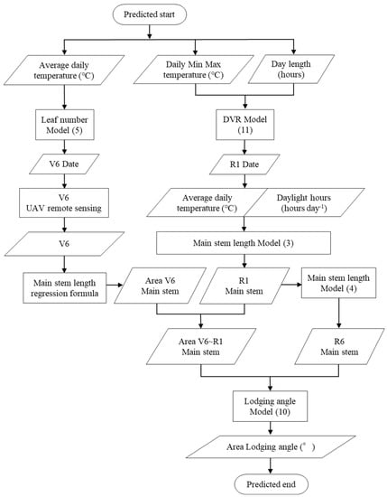
Figure 1.
Flowchart showing the protocol for the areal lodging prediction method.
- The calendar day of V6 was predicted using the leaf age model (5).
- The main stem length at V6 was estimated areally using the vegetation index calculated by UAV remote sensing at V6.
- The main stem length at R1 was predicted by the main stem elongation model (3), and the main stem elongation from V6 to R1 was predicted areally from the difference, with the main stem length at V6 estimated in 1.
- The main stem length at R6 was predicted by substituting the main stem length of R1 predicted in 3 into the main stem elongation model (4).
- The lodging was predicted areally by substituting the main stem elongation from V6 to R1 predicted in 3 and the main stem length at R6 predicted in 4 into the lodging model (10).
The calendar date of the blooming stage (R1) also needed to be predicted to predict the main stem length at R1. The calendar date of R1 was predicted based on the DVR model (11) by Nakano et al. [46].
In the DVR model (11), T is the mean of the daily maximum and minimum temperatures (°C), and L is the daylength time (h). Parameter G is the minimum number of days between the emergence and blooming stages (d). Th is the temperature at which the DVR is halved under a certain day length (°C), Lc is the critical day length at which development proceeds (h), and A and B are coefficients for temperature and day length.
The parameters of model (11) were obtained using data from the cropping pattern analysis test reported by the Organization Miyagi Prefectural Furukawa Agricultural Experiment Station. The parameters of the DVR model (11) were obtained using the “emergence date”, “blooming stage”, “daily maximum temperature”, “daily minimum temperature”, and “daylength time” at the test site from 2001 to 2021 (n = 22). The parameters were calculated using a solver in Microsoft Excel 2019. The parameters of the soybean varieties ‘Ryuho’, ‘Enrei’, and ‘Fukuyutaka’, as reported by Nakano et al., were used as the initial values for the parameters [46]. The one with the lowest RMSE between the estimated and measured values was used as the parameter for ‘Miyagishirome’. In the DVR model (12), G = 23.38, Th = 19.51, Lc = 15.51, A = 0.372, B = 1.075, and the RMSE of the test data (n = 12) was 1.1 days.
To test the applicability of this prediction method, we used data from research conducted in Osaki City in 2019 and in Osaki City and Kurihara City in 2022. The research fields in 2019 were on two levels (fields A and D in Table 3), and the sowing dates were 27 May, 6 June, and 17 June. The number of research sites at each sowing time was two for both fields A and D on 27 May, two for field A and four for field D on 6 June, and two for fields A and D on 17 June. The area of each site was 24 m2 (3.0 m × 8.0 m) or 48 m2 (6.0 m × 8.0 m). In 2022, the research fields in Osaki City were set at three levels (fields A, E, and F). The sowing dates were 25 May and 6 July in Osaki City and 23 June in Kurihara City. The number of research sites was three in Osaki City and six in Kurihara City. The area of each site ranged from 9.0 m2 (3.0 m × 3.0 m) to 16 m2 (4.0 m × 4.0 m) in Osaki City and 9.0 m2 (3.0 m × 3.0 m) in Kurihara City. The average of the research sites in each field was used as the data for the analysis.
UAV remote sensing was conducted in 2019 on 13 July (at the site sowed on 27 May), 19 July (at the site sowed on 6 June), and 26 July (at the site sowed on 17 June). In 2022, the survey was conducted in Osaki City on 11 July (at the site sowed on 25 May) and 9 August (at the site sowed on 6 July) and in Kurihara City on 19 July. UAV remote sensing and image analysis were conducted in the same way as described in Section 2.3.2. In Kurihara City, the date of the UAV remote sensing did not match the stage of V6. Therefore, the calendar date for V6 was determined by the leaf age model (5). The main stem length between the date of UAV remote sensing and V6 was calculated using the main stem elongation model (3) was used as a correction value. This correction value was then added to the main stem length estimated using UAV remote sensing.
The lodging angle was measured on R8 according to the method of triangular function, as reported by Konno and Homma [6]. We selected 1.5 m2 for a site area of 9.0, 16, and 24 m2 or 3.0 m2 for a site area of 48 m2 in areas with moderate growth and conducted research on three or six soybeans, respectively. The adaptability of the prediction method in this study was evaluated by comparing the lodging determinations measured with those made using the prediction method in this study. The meteorological data necessary for the various models were obtained from the Furukawa AMeDAS data station.
3. Results
3.1. Creation and Verification of Accuracy of Main Stem Elongation Model
A logistic regression (main stem elongation model (3) from emergence date to R1) using the integral of the temperature and daylight hour function f (Ti, Di) or the integral of temperature function f (Ti) was used as explanatory variables, which is shown in Figure 2. The temperature and daylight hour function f (Ti, Di) had an R2 of 0.94 (p < 0.001) and an RMSE of 4.2. The temperature function f (Ti) had an R2 of 0.88 (p < 0.001) and an RMSE of 5.7. In relation to the main stem length, the accumulated temperature and daylight hour function f (Ti, Di) had a higher R2 and lower RMSE and a stronger fit with the main stem length. The parameters of the main stem elongation model (3) with the temperature and daylight hours functions f (Ti, Di) as explanatory variables were a1 = 2.603, a2 = 0.085, b = 37.02, and c = 133.3. The parameters of the main stem elongation model for the temperature function f (Ti) were a2 = 0.133, b = 26.22, and c = 121.6. Comparing the parameters, a2 (rate of increase) was smaller, b (inflection point) was larger, and c (asymptote) was larger in the main stem elongation model (3).
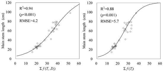
Figure 2.
Relationship between accumulated temperature and daylight hours functions f (Ti, Di) and temperature function f (Ti) and main stem length. Circles indicate the measured data and lines indicate logistic regressions.
The relationship between the main stem length at R1 and the main stem length peak was 0.95 (p < 0.001) for R2. This indicated that the main stem length peak could be estimated from the main stem length at R1 (Figure 3). The parameters of the main stem elongation model (4) were a3 = 0.83 and b2 = 31.8.
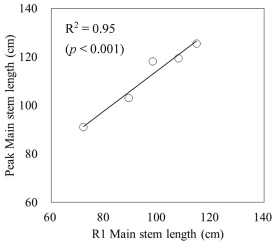
Figure 3.
Relationship between the main stem length at R1 and the peak main stem length. Circles indicate the measured data, and a line indicates the linear regression.
The accuracy verification of the main stem elongation model, which is a synthesis of the main stem elongation models (3) and (4) using test data, is shown in Figure 4. The RMSE between the predicted and measured values was 2.6 for the 25 May sowing in Osaki City, 9.1 for the 6 July sowing, and 4.3 in Kurihara City, with an average of 5.4 across the three plots.
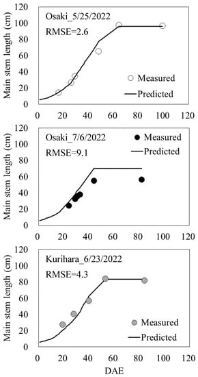
Figure 4.
Verification of accuracy of the main stem elongation model. DAE indicates days after emergence.
Figure 5 shows the accumulated air temperature and accumulated daylight hours for the years and regions for which the test data were obtained. Each test data set showed a different trend of accumulated air temperature and accumulated daylight hours. Accumulated temperatures were similar in all three plots until V8, after which the 25 May sowing in Osaki City had the highest accumulated temperatures. The 6 July sowing in Osaki City had lower accumulated temperatures from V8 to R1 than the other two plots, and the accumulated temperature at R6 was also lower. Kurihara City was in the middle of the other two plots until R3, but the difference with Osaki City’s 6 July sowing became smaller at R6. The accumulated daylight hours from V4 to R6 were highest for the 25 May sowing in Osaki City. Sowing on 6 July in Osaki City had the least accumulated daylight hours from V8 to R1 and the least accumulated daylight hours to R3, but at R6, the accumulated daylight hours were equal to those in Kurihara City.
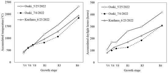
Figure 5.
Accumulated air temperature and accumulated daylight hours in the test data for the main stem elongation model.
3.2. Creation and Accuracy Verification of the Leaf Age Model
For the main stem node number model within the leaf age model (5), the R2 of the logistic regression using the accumulated values of the temperature function f (Ti) as explanatory variables was 0.96 (p < 0.001), and the RSME was 0.90 (Figure 6). The parameters of the main stem node number model were a4 = 0.094, b3 = 21.90, and c2 = 21.06. The accuracy of the leaf age model (5), which subtracted 2.5 from the main stem node number model, was verified using test data, and the RMSE between predicted and measured values was 0.6 (Figure 7).
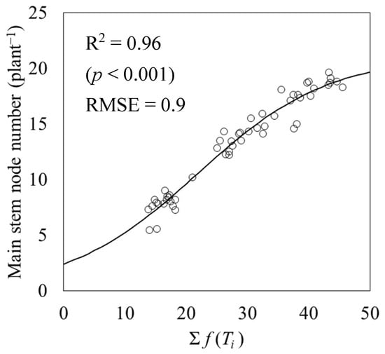
Figure 6.
Relationship between the accumulated temperature function f (Ti) and the number of main stem nodes. Circles indicate the measured data and a line indicates the logistic regression.
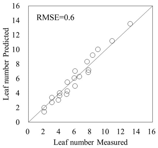
Figure 7.
Verification of accuracy of the leaf age model. Circles indicate the measured data and a line indicates the 1:1 line.
3.3. Estimation of Main Stem Length Using a Soil-Adjusted Vegetation Index That Takes Vegetation Coverage into Account
The minimum value of the measured main stem length was 24.9 cm, the maximum value was 69.4 cm, and the mean value was 45.0 cm (Figure 8). The minimum value for vegetation cover was 0.38, the maximum value was 0.85, and the mean value was 0.60. The minimum value for each vegetation index was 0.13 for SAVIvc, 0.60 for NDVI, 0.13 for SAVI, and 0.10 for MSAVI. The maximum values were 0.75 for SAVIvc, 0.93 for NDVI, 0.68 for SAVI, and 0.77 for MSAVI. The mean values were 0.44 for SAVIvc, 0.80 for NDVI, 0.41 for SAVI, and 0.39 for MSAVI. The maximum and minimum vegetation index values were higher for NDVI than for the soil-adjusted vegetation indices SAVIvc, SAVI, and MSAVI. When compared among the soil-adjusted vegetation indices, SAVI had the lowest maximum value, and the distribution of MSAVI tended to be skewed toward the lower values.
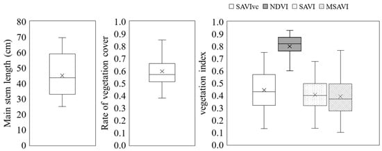
Figure 8.
Data used in the development of the method for estimating the main stem length using a soil-adjusted vegetation index that takes vegetation cover into account. × in the figure indicates the average value.
The relationship between each vegetation index and main stem length is shown in Table 4 and Figure 9. The vegetation index with the highest R2 was SAVIvc (R2 = 0.78, p < 0.001) proposed in this study. NDVI (R2 = 0.69, p < 0.001), SAVI (R2 = 0.62, p < 0.001), and MSAVI (R2 = 0.60, p < 0.001) were the next highest. Comparing the slope of the regression formula for SAVIvc and NDVI, the slope was 69.5 for SAVIvc and 120.7 for NDVI, with SAVIvc being smaller. The standard errors were 5.1 for SAVIvc and 11.1 for NDVI, with 95% confidence intervals ranging from 59.2 to 79.9 for SAVIvc and 98.4 to 143.0 for NDVI. The estimation error for SAVIvc was smaller.
Table 4.
Regression formulas and parameters for the main stem length at each vegetation index.
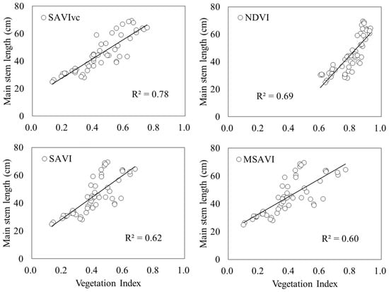
Figure 9.
Relationship between vegetation index and the main stem length. Circles indicate the measured data, and lines indicate the linear regressions.
3.4. Areal Lodging Prediction Method Combining Main Stem Elongation Model and Soil-Adjusted Vegetation Index
The predicted lodging angles by the main stem elongation models (3) and (4) in combination with the soil-adjusted vegetation index SAVIvc are shown in Table 5 and Figure 10. The leaf age model (5) predicted the calendar date of V6 to be 13 July for the 27 May sowing, 20 July for the 6 June sowing, and 27 July for the 17 June sowing in 2019. The model also predicted that to be 11 July for the 25 May sowing, 9 August for the 6 July sowing in Osaki City and 26 July for the sowing on 23 June in Kurihara City in 2022.
Table 5.
Results of lodging prediction using the areal lodging prediction method.
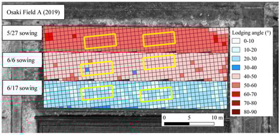
Figure 10.
Results of lodging prediction using the areal lodging prediction method. This figure shows field A in 2019. The yellow box in the figure indicates research sites.
The DVR model (12) predicted the calendar dates of R1 to be 5 August for the 27 May sowing, 8 August for the 6 June sowing, and 11 August for the 17 June sowing in 2019. The model also predicted that to be 1 August for the 25 May sowing, 20 August for the 6 July sowing in Osaki City and 10 August for the 23 June sowing in Kurihara City in 2022.
The main stem lengths at V6 (a in Table 5) estimated by SAVIvc were 21.6 to 23.9 cm for the 27 May sowing, 25.7 to 27.7 cm for the 6 June sowing and 35.8 to 43.9 cm for the 17 June sowing in 2019; in 2022, were 34.2 to 37.5 cm for the 25 May sowing, 30.5 to 30.8 cm for the 6 July sowing in Osaki City and 36.4 cm for the 23 June sowing in Kurihara City.
The main stem lengths at R1 (b in Table 5) predicted by the main stem elongation model (3) were 83.5 cm for the 27 May sowing, 77.2 cm for the 6 June sowing, and 63.2 cm for the 17 June sowing in 2019; in 2022, were 74.9 cm for the 25 May sowing, 46.4 cm for the 6 June sowing in Osaki City and 64.9 cm for the 23 June sowing in Kurihara City.
The main stem elongation from V6 to R1 calculated from the main stem lengths at V6 estimated by SAVIvc and the main stem lengths at R1 predicted by the main stem elongation model (3) was the highest at 59.7 to 62.0 cm for the 27 May sowing in 2019 and the lowest at 15.6 to 15.9 cm for the 6 June sowing in 2022.
The main stem lengths at R6 predicted by the main stem elongation model (4) were 100.9 cm for the 27 May sowing, 95.6 cm for the 6 June sowing, and 84.1 cm for the 17 June sowing in 2019; in 2022, were 93.7 cm for the 25 May sowing, 70.2 cm for the 6 June sowing in Osaki City and 85.5 cm for the 23 June sowing in Kurihara City.
In the 27 May sowing in 2019, when the highest main stem elongation from V6 to R1 and the highest main stem length at R6 main stem were predicted, the lodging angle was 59.0 to 60.8° and was predicted to be the largest. In the 6 June sowing in 2022, when the main stem elongation from V6 to R1 was predicted to be the lowest, and the main stem length at R6 was predicted to be the lowest, the lodging angle was 10.4 to 10.5° and no lodging was predicted to occur.
The RMSE between the predicted and measured lodging angles was 8.8 (Figure 11). The prediction error was greater in the 17 June sowing in 2019, but the error between prediction and measurement was smaller in the other plots.
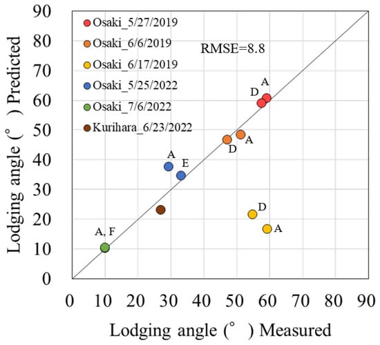
Figure 11.
Relationship between the predicted and measured lodging angles. Alphabets beside the plots indicate field IDs.
4. Discussion
4.1. Modeling of the Main Stem Length and Leaf Age
The temperature and daylight hours were considered in the modeling of the main stem length from V6 to R1. The inclusion of daylight hours in the model resulted in a higher R2 and lower RMSE and a better fit with the main stem length compared to only temperature. The peak main stem length could be estimated from the main stem length at R1. The accuracy of the composite model of main stem elongation models (3) and (4) was verified using test data from different years and regions. The RMSE was 5.3, which indicated that the models were generally accurate, including under different climatic conditions during the growing season. The RMSE of the leaf age model, which subtracted 2.5 from the number of main stem nodes, was 0.6 and was generally estimated with a relatively high level of accuracy.
In this study, the temperature function f (Ti) in the main stem elongation model of Nakano et al. was used for the main stem elongation model (3) from V6 to R1 [7]. Egli reported that individuals with higher main stem lengths had more main stem nodes [9]. Umezaki and Matsumoto also stated that the elongation pattern between each node follows an S-shaped curve [8]. This demonstrates the robustness of our model, which assumes an S-shaped increase in the main stem length as the number of main stem nodes increases. The estimation accuracy was improved by the main stem elongation model using the temperature and daylight hour function f (Ti, Di), which incorporates the daylight hours (Di) into the temperature function f (Ti) of Nakano et al. [7]. Regarding the relationship between daylight and the main stem length, the main stem length is higher under shading conditions and fewer daylight hours [10,11,12]. Morishita et al. reported that the formula for the relationship between daylight hours 15 days before the blooming stage and the main stem length was y = 94.3 − 0.224x (r = −0.553, p < 0.01) [10]. Comparing the main stem length (94.3 cm) when there were 0 daylight hours 15 days before the blooming stage with the main stem length (54.0 cm) when there were 180 daylight hours (12 h from 6:00 to 18:00 × 15 days), it was calculated that the main stem length was 1.8 times higher when daylight hours were 0 h. The term {1 + exp(−a1 × Di)} including daylight hours (Di) in the temperature and daylight hour function f (Ti, Di) in this study is 2.0 when daylight hour is 0. This indicates a twofold increase in main stem elongation, which is generally consistent with the report by Morishita et al. [10].
In terms of the main stem elongation model (4), the relationship between the main stem length at R1 and the main stem length of the peak has been shown to be similar. Heatherly and Smith (2004) reported that the main stem length elongated from R1 to stem termination (ST) in the finite elongation types tested [47]. There was a significant positive relationship between the main stem length at R1 and ST. ‘Miyagishirome’ was also a determinate type, and their report was consistent with the main stem elongation model (4) in this study. As shown in the results of Konno and Homma, the main stem length elongation from emergence to R1 was the largest, and the main stem length elongation from R1 to the peak was relatively small [6]. This suggests that individuals with higher main stem lengths at R1 would also have higher final main stem lengths.
For the leaf age model (5) in this study, the development of the nth leaf was assumed to occur when the n + 1 node was under extraction. Fehr has provided the criterion that the number of main stem nodes is based on counting the nodes where the leaves have developed [24]. At the time the nth leaf unfolds, the n + 1 node is not counted because the n + 1 leaf has not yet unfolded and is still under extraction. The leaf age model (5) in which leaf age is calculated by subtracting a total of 2.5 nodes, namely the cotyledonary node, primary leaf node, and the n + 1 node in the middle of extraction from the number of main stem nodes, was considered to be a model reflecting Fehr’s criteria [22].
4.2. Estimation of the Main Stem Length by Soil-Adjusted Vegetation Index Considering Vegetation Cover
This study showed that as a soil-adjusted vegetation index that takes vegetation cover into account, SAVIvc could be used to estimate main stem length with higher estimation accuracy than previous vegetation indices. A range of methods has been reported for estimating the above-ground dry matter weight using vegetation indices. As reported by Fehr, soybean growth proceeds by leaf unfolding at the main stem node [24]. Branching occurs as the number of main stem nodes increases [48]. These indicate that above-ground dry matter weight increases as the number of main stem nodes increases. The estimation of above-ground dry matter weight by the vegetation index reflects the variation in the number of main stem nodes. There is a positive relationship between the number of main stem nodes and the main stem length, suggesting that the vegetation index could be used to estimate the main stem length [9].
As highlighted by Huete, varying the soil adjustment term (L) in the soil-adjusted vegetation index with vegetation cover improved the accuracy of the growth rate estimates [20]. The poor accuracy of the estimation of SAVI and MSAVI, the previously reported soil-adjusted vegetation indices, may be due to the substantial variability in vegetation cover until the soybean reaches full vegetation cover. In this study, vegetation cover varied from 0.38 to 0.85. Therefore, the SAVI, in which L was set with a constant of 0.5, was considered less accurate than SAVIvc. This is because it was undercounted when vegetation cover was relatively low and overcounted when vegetation cover was relatively high. The poor relationship between SAVI and vegetation coverage was also reported at near-saturated vegetation coverage [49]. MSAVI is a modified version of SAVI: L of MSAVI is optimized by iterative calculation [21]. In the optimization, L was started from 1–SAVI, and the present equation was obtained after repeated calculation. Consequently, L in MSAVI is not obtained from actual measurements of vegetation coverage. On the other hand, SAVIvc in this study requires s the quantification of Lvc by binarizing the NIR images for each observation. Since binarization clearly separates vegetation and soil, SAVIvc is a better index to estimate the growth rate of soybean. Regarding L, Ren et al. reported that the highest accuracy was obtained in estimating above-ground living biomass in arid grasslands at a negative L [50]. They suggested that the negative value reduced the effect of soil noise ascribable to the width of a global soil line in sparse vegetation conditions. However, the condition in this study was soybean with uniform vegetation. Accordingly, we applied Lvc, ranging from 0 to 1.
NDVI without the soil adjustment term (L) was considered less accurate than SAVIvc because of reflections from the soil surface, as highlighted by Kamaki et al. [19]. The NDVI estimated the growth rate within a relatively narrow range because the baseline was higher than the soil-adjusted vegetation index due to reflections from the soil surface. Therefore, the larger slope of the regression formula was considered to have increased the standard error and 95% confidence interval, which decreased the accuracy of the estimation. The SAVIvc had the highest accuracy in estimating the main stem length because it reduced the challenges of the previously reported soil-adjusted vegetation indices (SAVI, MSAVI) and vegetation indices (NDVI).
4.3. Areal Lodging Prediction by Combining the Main Stem Elongation Model and Soil-Adjusted Vegetation Index
The areal lodging prediction method with the main stem elongation model and SAVIvc (areal main stem length estimation) was able to predict the lodging angle with an accuracy of RMSE = 8.8. This result demonstrates that there were no significant errors in the main stem length estimation by the main stem elongation models (3) and (4), the leaf age model (5), and SAVIvc in this study. However, there was a substantial error between the predicted and measured lodging angles for the 17 June sowing, shown in Figure 11. Konno and Homma indicated that the main stem elongation of V6 to R1 and the main stem length of R6 can explain the lodging angle [6]. However, they also noted that wind speed also affects the lodging angle. The maximum wind speed for R3 to R8 at the 17 June 2019 sowing used in the test data for this forecasting method was 7.3 m s−1, which is classified as a high wind speed in the Konno and Homma report [6]. The degree of lodging was predicted to be relatively small based on main stem elongation from V6 to R1 and R6 main stem length. However, the angle of lodging was larger than predicted because of the high wind speed conditions.
5. Conclusions
In this study, we predicted lodging on an areal basis by estimating the areal main stem length using a main stem elongation model and remote sensing. According to the lodging prediction model of Konno and Homma (Formula (10)), the main stem elongation model alone can predict lodging [6]. However, because the main stem elongation model is weather-dependent, the prediction results can only be shown as representative values. Therefore, areal main stem length estimation by SAVIvc was used at the starting point of lodging prediction. The method provides the prediction of lodging angles from an areal perspective by including the risk of lodging due to weather conditions during the growth. The areal perspective may also include differences in initial growth due to differences in soil physicochemical properties, etc. The purpose of lodging prediction is to determine the implementation of measures such as “pinching”. This prediction method, which visualizes lodging angles, facilitates the prioritization of measures in each field and within a field. It is hoped that the prediction method will enable farmers to evaluate the risk of lodging and take measures depending on cultivation management and field conditions.
Yamamoto et al. and Vieira et al. reported damage assessment methods for soybean using UAV remote sensing for red crown rot damage and dicamba damage, respectively [51,52], expecting the practical application of UAV to early pest control and breeding. These studies utilized machine learning for the assessment. For the lodging prediction, machine learning would be effective to in-corporates a variety of variables, such as wind speed and cultivar. Actually, the test data in this study included the effect of wind speed on lodging angle [6]. Given that it is difficult to predict wind speeds in the future, it is necessary to consider risk diversification by using not only native cultivars but also lodging-resistant cultivars in areas where wind speeds are high.
Author Contributions
T.K.: Conceptualization, Data curation, Formal analysis, Funding acquisition, Investigation, Methodology, Project administration, Resources, Supervision, Validation, Visualization, Writing—original draft, Writing—review and editing; K.H.: Supervision, Writing—review and editing. All authors have read and agreed to the published version of the manuscript.
Funding
This study was partially supported by the Takano Life Science Research Foundation, JSPS KAKENHI 21H02172 and JICA-JST SATREPS JPMJSA 1909. We would like to express our deepest gratitude.
Data Availability Statement
Data will be made available on request.
Acknowledgments
We would like to thank the staff of Technology Innovation Research and Development Unit, Kubota Corporation for their great cooperation in UAV remote sensing, including the loan of UAVs and instructions on how to use them. We also thank the staff of Organization Miyagi Prefectural Furukawa Agricultural Experiment Station for their cooperation in our research. We would like to express our deepest gratitude to them.
Conflicts of Interest
The authors declare no conflict of interest.
References
- Saitoh, K.; Nishimura, K.; Kitahara, T. Effect of Lodging on Seed Yield of Field-Grown Soybean—Artificial Lodging and Lodging Preventing Treatments. Jpn. J. Crop Sci. 2012, 81, 27–32. [Google Scholar] [CrossRef]
- Uchikawa, O.; Miyazaki, M.; Tanaka, K. The relationship between lodgingof soybean and the combine harvesting loss in Fukuoka Prefecture in 2004. Rep. Kyushu Branch Crop Sci. Soc. Jpn. 2006, 72, 32–34. [Google Scholar]
- Hayashi, M.; Hamada, Y.; Tani, T.; Hiraiwa, K. Development of Pinching Machine and Effect of Pinching for Soybean. Res. Bull. Aichi Agric. Res. Cent. 2009, 40, 93–97. [Google Scholar]
- Kakiuchi, J. Effects of Pinching on Growth and Yield of Different Soybean Cultivars. Jpn. J. Crop Sci. 2021, 90, 414–422. [Google Scholar] [CrossRef]
- Raza, A.; Asghar, M.A.; Ahmad, B.; Bin, C.; Iftikhar Hussain, M.; Li, W.; Iqbal, T.; Yaseen, M.; Shafiq, I.; Yi, Z.; et al. Agro-Techniques for Lodging Stress Management in Maize-Soybean Intercropping System—A Review. Plants 2020, 9, 1592. [Google Scholar] [CrossRef]
- Konno, T.; Homma, K. Impact Assessment of Main Stem Elongation and Wind Speed on Lodging of Soybean Cultivar ‘Miyagishirome’. Res. Sq. 2023; preprints. [Google Scholar] [CrossRef]
- Nakano, S.; Purcell, L.C.; Homma, K.; Shiraiwa, T. Modeling Leaf Area Development in Soybean (Glycine max L.) Based on the Branch Growth and Leaf Elongation. Plant Prod. Sci. 2020, 23, 247–259. [Google Scholar] [CrossRef]
- Umezaki, T.; Matsumoto, S. Studies on Internode Elongation in Soybean Plants: I. Internode Elongation Patterns of the Main Stem in Four Late Soybean Cultivars. Jpn. J. Crop Sci. 1989, 58, 364–367. [Google Scholar] [CrossRef]
- Egli, D.B. The Relationship between the Number of Nodes and Pods in Soybean Communities. Crop Sci. 2013, 53, 1668–1676. [Google Scholar] [CrossRef]
- Morishita, M.; Hirano, T.; Miyamoto, Y. Effect of Sunshine Hours on Main Stem Length in Soybean. Bull. Wakayama Prefect. Agric. Exp. Stn. 1986, 11, 9–12. [Google Scholar] [CrossRef]
- Liu, X.; Rahman, T.; Song, C.; Su, B.; Yang, F.; Yong, T.; Wu, Y.; Zhang, C.; Yang, W. Changes in Light Environment, Morphology, Growth and Yield of Soybean in Maize-Soybean Intercropping Systems. Field Crops Res. 2017, 200, 38–46. [Google Scholar] [CrossRef]
- Feng, L.; Raza, M.A.; Li, Z.; Chen, Y.; Khalid, M.H.B.; Du, J.; Liu, W.; Wu, X.; Song, C.; Yu, L.; et al. The Influence of Light Intensity and Leaf Movement on Photosynthesis Characteristics and Carbon Balance of Soybean. Front. Plant Sci. 2019, 9, 1952. [Google Scholar] [CrossRef]
- Taki, S.; Kujira, Y. Effects of Different Soil Condition on Growth of Soybean Cv. Enrei. Hokuriku Crop Sci. 2009, 44, 41–45. [Google Scholar] [CrossRef]
- Morishita, M.; Ishitsuka, N. Estimation of Soil Properties Distribution Using UAV Observation and Machine Learning. J. Jpn. Agric. Syst. Soc. 2021, 37, 21–28. [Google Scholar] [CrossRef]
- Zhang, L.; Hashimoto, N.; Saito, Y.; Obara, K.; Ishibashi, T.; Ito, R.; Yamamoto, S.; Maki, M.; Homma, K. Validation of Relation between SPAD and Rice Grain Protein Content in Farmer Fields in the Coastal Area of Sendai, Japan. AgriEngineering 2023, 5, 369–379. [Google Scholar] [CrossRef]
- Yamamoto, S.; Homma, K.; Hashimoto, N.; Maki, M. Evaluation of Excess Soil Moisture Damage on Soybean Grown in Farmer’s Fields by UAV Remote-Sensing. Jpn. J. Crop Sci. 2019, 88, 48–49. [Google Scholar] [CrossRef]
- Gitelson, A.A.; Kaufman, Y.J.; Merzlyak, M.N. Use of a Green Channel in Remote Sensing of Global Vegetation from EOS-MODIS. Remote Sens. Environ. 1996, 58, 289–298. [Google Scholar] [CrossRef]
- Tambo, A.; Shimada, M.; Yoshifuji, A.; Imamoto, Y.; Nagahata, H.; Fujihara, Y.; Tsukaguchi, T. Analysis of Soybean Seed Yield Using Vegetation Index Captured with UAV. Jpn. J. Crop Sci. 2021, 90, 261–268. [Google Scholar] [CrossRef]
- Kamaki, S.; Nakamoto, S.; Hoh, D.; Inamura, T.; Inoue, H. Estimation of Dry Matter Weight of Soybean Using the New Vegetation Index. J. Crop Res. 2021, 66, 47–53. [Google Scholar] [CrossRef]
- Huete, A.R. A Soil-Adjusted Vegetation Index (SAVI). Remote Sens. Environ. 1988, 25, 295–309. [Google Scholar] [CrossRef]
- Qi, J.; Chehbouni, A.; Huete, A.R.; Kerr, Y.H.; Sorooshian, S. A Modified Soil Adjusted Vegetation Index. Remote Sens. Environ. 1994, 48, 119–126. [Google Scholar] [CrossRef]
- Takizawa, H. Relationship between Internode Length and Crop Management of Leading Soybean Variety in Miyagi Prefecture. Tohoku Agric. Res. 2006, 59, 73–74. [Google Scholar]
- Ministry of Agriculture, Forestry and Fisheries of Japan. Characteristics of Japanese Soybean Varieties. Available online: https://www.maff.go.jp/j/seisan/ryutu/daizu/d_ziten/attach/pdf/index-1.pdf (accessed on 1 June 2023).
- Fehr, W.R. Stages of Soybean Development. Iowa State Univ. Spec. Rep. 1977, 80, 1–12. [Google Scholar]
- Organization Miyagi Prefectural Furukawa Agricultural Experiment Station. Cropping Pattern Analysis Test of Paddy Rice, Soybeans and Wheat Crops in Miyagi Prefecture in 2005; Extraordinary Report of Organization Miyagi Prefectural Furukawa Agricultural Experiment Station; Organization Miyagi Prefectural Furukawa Agricultural Experiment Station: Miyagi, Japan, 2006; Volume 3. [Google Scholar]
- Organization Miyagi Prefectural Furukawa Agricultural Experiment Station. Cropping Pattern Analysis Test of Paddy Rice, Soybeans and Wheat Crops in Miyagi Prefecture in 2006; Extraordinary Report of Organization Miyagi Prefectural Furukawa Agricultural Experiment Station; Organization Miyagi Prefectural Furukawa Agricultural Experiment Station: Miyagi, Japan, 2007; Volume 4. [Google Scholar]
- Organization Miyagi Prefectural Furukawa Agricultural Experiment Station. Cropping Pattern Analysis Test of Paddy Rice, Soybeans and Wheat Crops in Miyagi Prefecture in 2007; Extraordinary Report of Organization Miyagi Prefectural Furukawa Agricultural Experiment Station; Organization Miyagi Prefectural Furukawa Agricultural Experiment Station: Miyagi, Japan, 2008; Volume 5. [Google Scholar]
- Organization Miyagi Prefectural Furukawa Agricultural Experiment Station. Cropping Pattern Analysis Test of Paddy Rice, Soybeans and Wheat Crops in Miyagi Prefecture in 2008; Extraordinary Report of Organization Miyagi Prefectural Furukawa Agricultural Experiment Station; Organization Miyagi Prefectural Furukawa Agricultural Experiment Station: Miyagi, Japan, 2009; Volume 6. [Google Scholar]
- Organization Miyagi Prefectural Furukawa Agricultural Experiment Station. Cropping Pattern Analysis Test of Paddy Rice, Soybeans and Wheat Crops in Miyagi Prefecture in 2009; Extraordinary Report of Organization Miyagi Prefectural Furukawa Agricultural Experiment Station; Organization Miyagi Prefectural Furukawa Agricultural Experiment Station: Miyagi, Japan, 2010; Volume 7. [Google Scholar]
- Organization Miyagi Prefectural Furukawa Agricultural Experiment Station. Cropping Pattern Analysis Test of Paddy Rice, Soybeans and Wheat Crops in Miyagi Prefecture in 2010; Extraordinary Report of Organization Miyagi Prefectural Furukawa Agricultural Experiment Station; Organization Miyagi Prefectural Furukawa Agricultural Experiment Station: Miyagi, Japan, 2011; Volume 8. [Google Scholar]
- Organization Miyagi Prefectural Furukawa Agricultural Experiment Station. Cropping Pattern Analysis Test of Paddy Rice, Soybeans and Wheat Crops in Miyagi Prefecture in 2011; Extraordinary Report of Organization Miyagi Prefectural Furukawa Agricultural Experiment Station; Organization Miyagi Prefectural Furukawa Agricultural Experiment Station: Miyagi, Japan, 2012; Volume 9. [Google Scholar]
- Organization Miyagi Prefectural Furukawa Agricultural Experiment Station. Cropping Pattern Analysis Test of Paddy Rice, Soybeans and Wheat Crops in Miyagi Prefecture in 2012; Extraordinary report of Organization Miyagi Prefectural Furukawa Agricultural Experiment Station; Organization Miyagi Prefectural Furukawa Agricultural Experiment Station: Miyagi, Japan, 2013; Volume 10. [Google Scholar]
- Organization Miyagi Prefectural Furukawa Agricultural Experiment Station. Cropping Pattern Analysis Test of Paddy Rice, Soybeans and Wheat Crops in Miyagi Prefecture in 2013; Extraordinary Report of Organization Miyagi Prefectural Furukawa Agricultural Experiment Station; Organization Miyagi Prefectural Furukawa Agricultural Experiment Station: Miyagi, Japan, 2014; Volume 11. [Google Scholar]
- Organization Miyagi Prefectural Furukawa Agricultural Experiment Station. Cropping Pattern Analysis Test of Paddy Rice, Soybeans and Wheat Crops in Miyagi Prefecture in 2014; Extraordinary Report of Organization Miyagi Prefectural Furukawa Agricultural Experiment Station; Organization Miyagi Prefectural Furukawa Agricultural Experiment Station: Miyagi, Japan, 2015; Volume 12. [Google Scholar]
- Organization Miyagi Prefectural Furukawa Agricultural Experiment Station. Cropping Pattern Analysis Test of Paddy Rice, Soybeans and Wheat Crops in Miyagi Prefecture in 2015; Extraordinary Report of Organization Miyagi Prefectural Furukawa Agricultural Experiment Station; Organization Miyagi Prefectural Furukawa Agricultural Experiment Station: Miyagi, Japan, 2016; Volume 13. [Google Scholar]
- Organization Miyagi Prefectural Furukawa Agricultural Experiment Station. Cropping Pattern Analysis Test of Paddy Rice, Soybeans and Wheat Crops in Miyagi Prefecture in 2016; Extraordinary Report of Organization Miyagi Prefectural Furukawa Agricultural Experiment Station; Organization Miyagi Prefectural Furukawa Agricultural Experiment Station: Miyagi, Japan, 2017; Volume 14. [Google Scholar]
- Organization Miyagi Prefectural Furukawa Agricultural Experiment Station. Cropping Pattern Analysis Test of Paddy Rice, Soybeans and Wheat Crops in Miyagi Prefecture in 2017; Extraordinary Report of Organization Miyagi Prefectural Furukawa Agricultural Experiment Station; Organization Miyagi Prefectural Furukawa Agricultural Experiment Station: Miyagi, Japan, 2018; Volume 15. [Google Scholar]
- Organization Miyagi Prefectural Furukawa Agricultural Experiment Station. Cropping Pattern Analysis Test of Paddy Rice, Soybeans and Wheat Crops in Miyagi Prefecture in 2018; Extraordinary Report of Organization Miyagi Prefectural Furukawa Agricultural Experiment Station; Organization Miyagi Prefectural Furukawa Agricultural Experiment Station: Miyagi, Japan, 2019; Volume 16. [Google Scholar]
- Organization Miyagi Prefectural Furukawa Agricultural Experiment Station. Cropping Pattern Analysis Test of Paddy Rice, Soybeans and Wheat Crops in Miyagi Prefecture in 2019; Extraordinary Report of Organization Miyagi Prefectural Furukawa Agricultural Experiment Station; Organization Miyagi Prefectural Furukawa Agricultural Experiment Station: Miyagi, Japan, 2020; Volume 17. [Google Scholar]
- Organization Miyagi Prefectural Furukawa Agricultural Experiment Station. Cropping Pattern Analysis Test of Paddy Rice, Soybeans and Wheat Crops in Miyagi Prefecture in 2020; Extraordinary Report of Organization Miyagi Prefectural Furukawa Agricultural Experiment Station; Organization Miyagi Prefectural Furukawa Agricultural Experiment Station: Miyagi, Japan, 2021; Volume 18. [Google Scholar]
- Organization Miyagi Prefectural Furukawa Agricultural Experiment Station. Cropping Pattern Analysis Test of Paddy Rice, Soybeans and Wheat Crops in Miyagi Prefecture in 2021; Extraordinary Report of Organization Miyagi Prefectural Furukawa Agricultural Experiment Station; Organization Miyagi Prefectural Furukawa Agricultural Experiment Station: Miyagi, Japan, 2022; Volume 19. [Google Scholar]
- Japan Meteorological Agency Download Historical Weather Data. Available online: https://www.jma.go.jp/jma/index.html (accessed on 1 June 2023).
- Rouse, J.W.; Haas, R.H.; Schell, J.A.; Deering, D.W.; Haas, R.H.; Schell, J.A.; Deering, D.W. Monitoring Vegetation Systems in the Great Plains with ERTS. In Proceedings of the Third Earth Resources Technology Satellite-1 Symposium, Washington, DC, USA, 10–14 December 1973; National Aeronautics and Space Administration: Washington, DC, USA, 1974; Volume 1. [Google Scholar]
- Otsu, N. A Threshold Selection Method from Gray-Level Histograms. IEEE Trans. Syst. Man Cybern. 1979, 9, 62–66. [Google Scholar] [CrossRef]
- Miyagi Prefecture Government Agricultural Administration Department. Growth Control Method of Soybean Variety “Miyagishirome” by Pinching Treatment. Available online: https://www.pref.miyagi.jp/soshiki/res_center/fukyugi96no1.html (accessed on 1 June 2023).
- Nakano, S.; Kumagai, E.; Shimada, S.; Sameshima, R.; Ohno, H.; Homma, K.; Shiraiwa, T. Modeling of Phenological Development Stages and Impact of Elevated Air Temperature on the Phenological Development of Soybean Cultivars in Japan. Jpn. J. Crop Sci. 2015, 84, 408–417. [Google Scholar] [CrossRef]
- Heatherly, L.G.; Smith, J.R. Effect of soybean stem growth habit on height and node number after beginning bloom in the Midsouthern USA. Crop Sci. 2004, 44, 1855–1858. [Google Scholar] [CrossRef]
- Torigoe, Y.; Shinji, H.; Kurihara, H. Studies on Developmental Morphology and Yield Determining Process in Soybeans: I. Relationship between Internode Elongation of the Main Stem and Branch Develoment. Jpn. J. Crop Sci. 1981, 50, 191–198. [Google Scholar] [CrossRef]
- Purevdorj, T.S.; Tateishi, R.; Ishiyama, T.; Honda, Y. Relationships between Percent Vegetation Cover and Vegetation Indices. Int. J. Remote Sens. 1998, 19, 3519–3535. [Google Scholar] [CrossRef]
- Ren, H.; Zhou, G.; Zhang, F. Using Negative Soil Adjustment Factor in Soil-Adjusted Vegetation Index (SAVI) for Aboveground Living Biomass Estimation in Arid Grasslands. Remote Sens. Environ. 2018, 209, 439–445. [Google Scholar] [CrossRef]
- Yamamoto, S.; Nomoto, S.; Hashimoto, N.; Maki, M.; Hongo, C.; Shiraiwa, T.; Homma, K. Monitoring Spatial and Time-Series Variations in Red Crown Rot Damage of Soybean in Farmer Fields Based on UAV Remote Sensing. Plant Prod. Sci. 2023, 26, 36–47. [Google Scholar] [CrossRef]
- Vieira, C.C.; Sarkar, S.; Tian, F.; Zhou, J.; Jarquin, D.; Nguyen, H.T.; Zhou, J.; Chen, P. Differentiate Soybean Response to Off-Target Dicamba Damage Based on UAV Imagery and Machine Learning. Remote Sens. 2022, 14, 1618. [Google Scholar] [CrossRef]
Disclaimer/Publisher’s Note: The statements, opinions and data contained in all publications are solely those of the individual author(s) and contributor(s) and not of MDPI and/or the editor(s). MDPI and/or the editor(s) disclaim responsibility for any injury to people or property resulting from any ideas, methods, instructions or products referred to in the content. |
© 2023 by the authors. Licensee MDPI, Basel, Switzerland. This article is an open access article distributed under the terms and conditions of the Creative Commons Attribution (CC BY) license (https://creativecommons.org/licenses/by/4.0/).