Abstract
Floods are some of the most devastating crop disasters in Southeast Asia. The Pampanga River Basin in the Philippines is a representative flood-prone area, where cultivation patterns vary according to the flood risk. However, quantitative analyses of the effects of flooding on cultivation patterns remain quite limited. Accordingly, this study analyzed MODIS LAI data (MCD15A2H) from 2007 to 2022 to evaluate annual and geographical differences in cultivation patterns in the Candaba municipality of the basin. The analysis consisted of two stages of hierarchical clustering: a first stage for area classification and a second stage for the classification of annual LAI dynamics. As a result, Candaba was divided into four areas, which were found to be partly consistent with the observed flood risk. Subsequently, annual LAI dynamics for each area were divided into two or three clusters. Obvious differences among clusters were caused by flooding in the late rainy season, which delayed the start of planting in the dry season. Clusters also indicated that cultivation patterns slightly changed over the 16 years of the study period. The results of this study suggest that the two-stage clustering approach provided an effective tool for the analysis of MODIS LAI data when considering cultivation patterns characterized by annual and geographical differences.
1. Introduction
Floods are some of the most devastating disasters, causing significant damage to crops around the world. The FAO has announced that damages to crops and livestock caused by flooding amounted to USD 21 billion, comprising 19% of the total loss caused by all disasters from 2008 to 2018 [1]. In order to reduce associated damages, cultivation patterns are varied depending on the flood risk in the floodplains of Southeast Asia [2,3]. Information about cultivation patterns is extremely important for the management and evaluation of flood damage [4]. At present, such information is mainly collected through field surveys. However, field surveys mostly fail to provide the geographical distribution of cultivation patterns, as they are conducted on a points basis. Moreover, surveys ordinarily consider a certain management period or growth stage, for example, the planting period or heading stage of cereals. These information constraints limit the ability to evaluate flood damage based on the crop growth stage or inundation depth.
The Pampanga River Basin is located in the central part of Luzon Island in the Philippines, and is one of the largest floodplains and rice-producing areas in Southeast Asia. Floods are frequently caused by monsoons and typhoons during the rainy season, affecting crops in various ways almost every year. For example, during Typhoon “Ulysses, 4490 hectares of farmland were damaged throughout the entire province of Pampanga, with agricultural damage amounting to about PHP 200 million (about USD 3.8 million) [5]. To avoid these damages, farmers have developed various cultivation patterns, including fish raising and vegetable cultivation [6]; however, the geographic distribution and annual change in cultivation patterns has not yet been analyzed. Such an analysis would provide important information, help evaluate how farmers have adapted to flooding and help develop countermeasures for the future. For example, farmers could consider their responses and the government could develop a regional strategy based on the flood risk. These scientific countermeasures may also increase resilience to future floods associated with climate change.
Remote sensing using satellite images has been considered as an alternative evaluation method to field surveys due to the versatility and wide applicability of the obtained information. Vegetation indices or the leaf area index (LAI) obtained from satellite images have been employed for the evaluation of crop growth [7,8], growth stage [9,10], and cultivation management [11]. In addition, various applications have been tested as evaluation methods, ranging from statistical methods, such as linear regression [12], to deep learning [13]. Coarse resolution and cloud disturbances are major constraints for the utilization of satellite images [14]; however, previous studies have suggested that the use of statistical procedures on long-term time-series data allow for the detection of changes in cultivation patterns. In 2021, Iwahashi et al. used time-series data from the MODIS LAI product to reveal conversion from late-matured to early-matured cultivars and extension of dry season rice cropping in Cambodia [15]. In 2022, Zhao et al. used long-term time-series data from the MODIS EVI product to reveal the effect of global warming on the phenological changes of wheat in China [16]. Based on the above information, we evaluated annual and geographical differences in cultivation patterns in the Pampanga River Basin, the Philippines, by analyzing long-term time-series MODIS data.
2. Materials and Methods
2.1. Study Area
This study was conducted in the Candaba municipality (15°05′N, 120°49′E), located in the floodplain of the Pampanga River Basin (Figure 1). The area is characterized by a tropical monsoon climate (Am). The rainy season is generally from June to October, during which typhoons of various sizes occur in the area. In the rainy season, several rivers flowing into the area often flood, especially during typhoon events. These floods transform some areas, through inundation, into a complex comprising variably saturated wetland, shallow swamps, and deeper freshwater ponds [17].
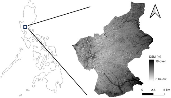
Figure 1.
The location of the Municipality of Candaba. The right figure shows a digital surface model (DSM) of Candaba (ALOS DSM: Global 30 m v3.2).
Candaba belongs to Region III (Central Luzon), and is one of the largest rice-producing areas in the Philippines [18]. Rice is the dominant crop in Candaba, but other modes of cultivation, including fish and vegetable cultivation, have also been reported [6]. The cultivation periods and times for rice vary, depending on flood and dry cultivation.
2.2. LAI Data
MODIS data (MCD15A2H) provided by NASA were downloaded for the 16 years from 2007 to 2022. MCD15A2H provides Leaf Area Index (LAI) values with 500 m pixel size every 8 days. The Leaf Area Index defined the one-sided green leaf area per unit ground area. This product estimates the LAI using a main look-up-table (LUT)-based procedure that exploits the spectral information content of MODIS red (648 nm) and near-infra-red (NIR) (858 nm) surface reflectance, and a back-up algorithm that uses empirical relationships between the Normalized Difference Vegetation Index (NDVI) and the canopy LAI and FPAR [19]. In this study, the 2013 version of GLCNMO, a raster data set that contains global land-cover information from supervised classification based on MODIS data with 500 m pixel size, was used to identify paddy fields. These data were developed by the secretariat of ISCGM in collaboration with the Geospatial Information Authority of Japan (GSI), Chiba University, and NGIAs of respective countries and regions [20]. LAI values were extracted from pixels in MCD15A2H that were identified as paddy fields according to GLCNMO. As the positions of GLCNMO and MCD15A2H do not necessarily match, the average of LAI values of all MCD15A2H pixels in the range of GLCNMO pixels was used as the LAI of the pixels.
2.3. Analysis of LAI Dynamics
In this study, hierarchical clustering was performed on extracted LAI data to group based on similarities. Among several clustering techniques, hierarchical clustering was selected due to its efficiency when data trends are unknown in advance. The cluster analysis was conducted in two stages (Figure 2). In the first stage, hierarchical clustering was performed on the time-series LAI data for 16 years in each pixel (n = 618), in order to classify areas with similar LAI dynamics. In the second stage, hierarchical clustering was performed on the time-series LAI data for one year in each pixel of each area classified in the first stage of hierarchical clustering (n = number of pixels in the area × 15). One-year data were divided from October of the previous year to September of the target year, in order to include planting periods of dry and rainy seasons. Ward’s method was employed to calculate the distance between clusters. The thresholds used to determine clusters were set at 60% and 70% of all Euclidean distances in the first and second stages, respectively.
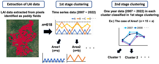
Figure 2.
Workflow of analysis methods used in this study. The red pixels in the left image were identified as paddy fields based on GLCNMO.
2.4. Software
MCD15A2H was downloaded using Google Earth Engine (Google Earth Engine, Python API version 0.1.330). Google Earth Engine is a cloud-based geospatial analysis platform that enables users to visualize and analyze satellite images of our planet [21]. LAI data extraction from MCD15A2H was performed using Quantum Geographic Information System (QGIS version 3.14). QGIS is a free, open software that allows users to create, edit, visualize, analyze, and publish geospatial data. After a shape file was created for each pixel of GLCNMO, the average LAI was extracted for each range of shape. Hierarchical clustering was performed using the SciPy library in Python (SciPy version 1.7.1).
3. Results
3.1. Area Classification in Candaba
First, hierarchical clustering was performed using the MODIS LAI product (MCD15A2H) for the 16 years of the study period (2007–2022). The first stage clearly classified Candaba into four areas: the southern area (Area 1), the northern area (Area 2), the lower terrain area (Area 3), and the eastern and western area (Area 4) (see Figure 3).
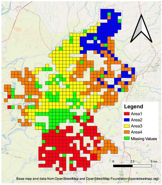
Figure 3.
The result of the first stage of hierarchical clustering using MODIS LAI products (2007–2022).
3.2. Annual LAI Dynamics for Each Region
The second stage of hierarchical clustering was performed using MODIS LAI data to compare annual LAI dynamics for each area and year. The results of clustering by year for each area follow. Different LAI dynamics are presented for each area.
3.2.1. Area 1 (Southern Area)
Area 1 was divided into two clusters. Figure 4 shows the averaged LAI dynamic for each cluster. Both clusters had a large peak during the dry season. Cluster 2 reached its peak earlier than Cluster 1, and the LAI value at the peak was higher than that of Cluster 1’s value at the peak. A small peak after the large peak was observed in Cluster 2, and the small peak occurred around the end of the dry season. Figure 5 shows the annual distribution of each cluster. Cluster 1 was frequently observed after 2015, while Cluster 2 was frequently observed before 2014.
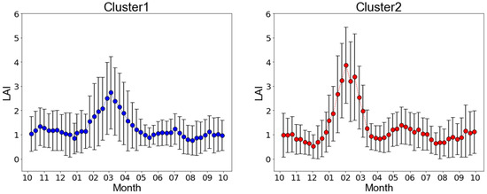
Figure 4.
Averaged LAI dynamics for each cluster in Area 1. Clusters were divided in the second stage of hierarchical clustering. Error bars show standard deviations.
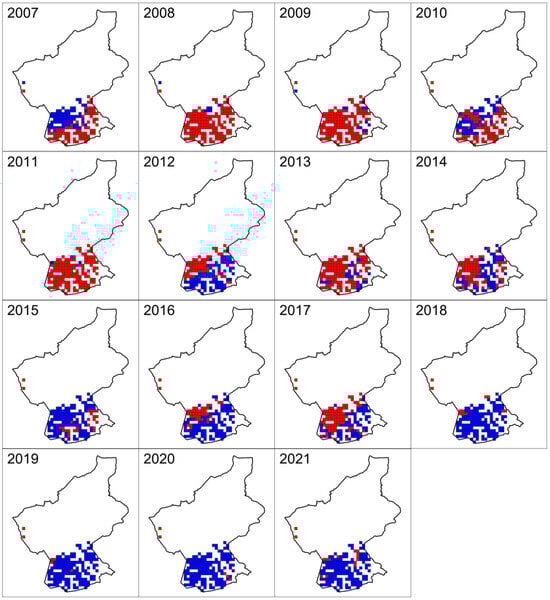
Figure 5.
The distribution map for each cluster in Area 1. Blue and red indicate Cluster 1 and Cluster 2 in Figure 4, respectively.
3.2.2. Area 2 (Northern Area)
Area 2 was divided into three clusters. Figure 6 shows the averaged LAI dynamics for each cluster. All clusters had three peaks throughout the year. Cluster 2 reached its first peak earlier than the other two clusters. Meanwhile, Cluster 3 reached its first peak later than the other two clusters, but its LAI value was significantly higher than those of the other two clusters. Figure 7 shows the annual distribution of each cluster. The northern part of the area was occupied by Cluster 1 and Cluster 3 from 2007 to 2022, while the southern part of the area transitioned from Cluster 1 to Cluster 2 around 2014.
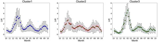
Figure 6.
Averaged LAI dynamics for each cluster in Area 2. Clusters were divided in the second stage of hierarchical clustering. Error bars show standard deviations.
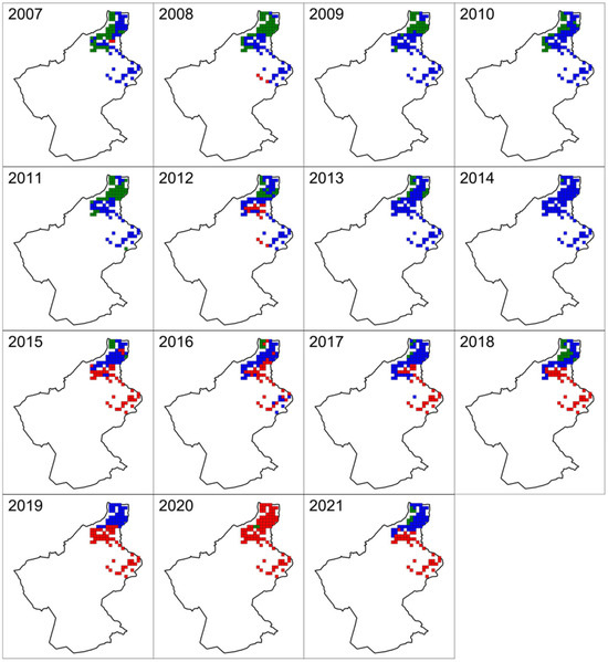
Figure 7.
The distribution map for each cluster in Area 2. Blue, red, and green indicate Cluster 1, 2, and 3 in Figure 6, respectively.
3.2.3. Area 3 (Lower Terrain Area)
Area 3 was divided into three clusters. Figure 8 shows the averaged LAI dynamics for each cluster. All clusters experienced a large peak during the dry season (first peak) and an additional peak just before the rainy season (second peak). Cluster 3 reached its first peak earlier than the other clusters. Cluster 2 was the latest to reach it’s peak, and had a small peak before its first peak. The LAI value at the second peak of Cluster 3 was higher than that of Cluster 2. Figure 9 shows the annual distribution of each cluster. Cluster 1 occupied the whole area until 2013, while Cluster 3 was more frequently observed after 2014. Cluster 2 occupied the entire area in 2015 and 2020.
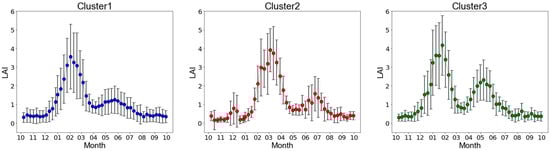
Figure 8.
Averaged LAI dynamics for each cluster in Area 3. Clusters were divided in the second stage of hierarchical clustering. Error bars show standard deviations.
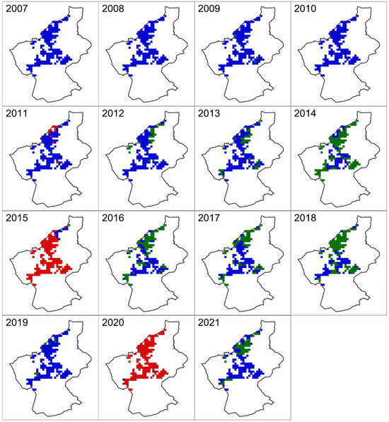
Figure 9.
The distribution map for each cluster in Area 3. Blue, red, and green indicate Cluster 1, 2, and 3 in Figure 8, respectively.
3.2.4. Area 4 (Eastern and Western Area)
Area 4 was divided into three clusters. Figure 10 shows the averaged LAI dynamics of each cluster. The LAI value of Cluster 1 fluctuated between one and two throughout the year. Cluster 2 had two peaks: August–September and December–January. Cluster 3 had a single peak, in February–March. Figure 11 shows the annual distribution of each cluster. The western area was occupied by Cluster 1 and Cluster 3 from 2007 to 2021. On the other hand, except for years between 2010 to 2012, most of the eastern area was occupied by Cluster 2.
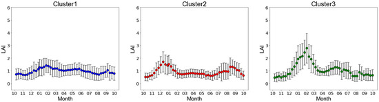
Figure 10.
Averaged LAI dynamics for each cluster in Area 4. Clusters were divided in the second stage of hierarchical clustering. Error bars show standard deviations.
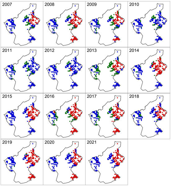
Figure 11.
The distribution map for each cluster in Area 4. Blue, red, and green indicate Cluster 1, 2, and 3 in Figure 10, respectively.
4. Discussion
In this study, in order to reveal differences in the annual LAI dynamics in Candaba, a two-stage clustering analysis was applied: the first stage involved the classification of area, while the second stage involved the classification of annual LAI dynamics. Direct clustering analysis of annual LAI dynamics without area classification did not yield obvious hierarchical structure corresponding to geographical distribution (Figure 12). As LAI data for a pixel may include outliers and/or errors, the observation of annual LAI dynamics patterns is often noisy. Increasing the dimensionality by combining 16 years of time-series data allowed for analysis of geographical differences in LAI dynamics, thus increasing similarity by dividing areas showing similar annual patterns.

Figure 12.
Differences in hierarchical structure between direct clustering analysis and two-stage clustering analysis. Different colors represent clusters divided by thresholds.
In the first stage of classification, Candaba was divided into four areas. As time-series LAI data were extracted for paddy fields, these areas may reflect local rice cultivation patterns. Classified areas were partly consistent with the geography (Figure 1) and flood areas under the influence of a typhoon (Figure 13). As the timing of cultivation depends on the flood risk in Candaba [6], a map similar to that shown in Figure 3 may be produced by combining the flood risk determined by topography with the experience of farmers. Area 4 presented lower LAI values and obscure peaks, suggesting that rice cultivation was not dominant in this area. This result was expected, as Area 4 occupies relatively higher terrain, where upland crops are sometimes planted (personal communications). Further analysis utilizing finer resolution satellite data may be required to obtain more precise results.
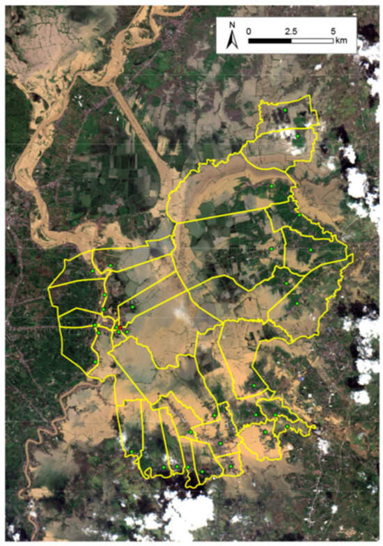
Figure 13.
Flood conditions after Typhoon Ulysses. This image was obtained from Sentinel-2 on 13 November 2020. Yellow lines indicate the barangay boundaries. The red dot indicates the location of Candaba municipal offices, and the green dots indicate the location of the barangay hall of each barangay. Barangay is the smallest local government unit that constitutes cities and municipalities in the Philippines.
In the second stage of classification, annual LAI dynamics in each area were divided into two or three clusters. One of the major differences among the clusters was the time of the first (and largest) peak, which seems to reflect the beginning of planting. An earlier first planting generally produced higher second and third peaks. As farmers wait to plant until the flood risk is low, the distribution of clusters may be governed by the flood condition during the rainy season. In particular, Cluster 2 in Area 3, which widely occupied the area in 2015 and 2020 (Figure 9), probably indicates that the rice was damaged and delayed by one month when compared to the other clusters: a small peak just before the dry season peak might mean that farmers started cultivation as usual each year, but it failed due to flooding; they may have restarted cultivation after flooding, which caused about a one month delay of the dry season peak (Figure 8). Notably, 2015 and 2020 were years that suffered from typhoon damage between November and December. In 2015, typhoon “Nona” passed through the area from 12 to 17 December, and 17 barangays were damaged by flooding [22]. In 2020, typhoon “Ulysses” passed through the area from 8 to 13 November, and 29 barangays were damaged by flooding [5]. According to the agricultural department of the municipal office of Candaba, these typhoons caused a delay in planting during the dry season (personal communications), consistent with the observed LAI dynamics.
Although the largest peak was observed in the dry season, this does not necessarily mean that the area and production of the dry season crop were higher than those in the rainy season. In fact, rainy season crops are also cultivated in areas with low flood risk [6]. The reason why the peak in the dry season appeared to be stronger than that in the rainy season may be that satellite observations are more likely to be disturbed by clouds in the rainy season [23]. Deeply submerged water also disturbs satellite observations [24]. Furthermore, cultivation in the dry season is more likely to be aligned due to inundation at the end of rainy season, which may be another reason for the enhanced peak observed in the dry season. Accordingly, the tendency of lower peaks in the rainy season may be due to the lower accuracy of the LAI product and the inconsistency of cultivation periods in the same pixel. Melendres (2014) has reported that rice is usually cultivated twice a year in Candaba, but only once in the heart of Candaba Swamp, due to flooding in the rainy season [25]. However, annual LAI dynamics showed one, three, and two peaks per year in Areas 1, 2, and 3, respectively. This inconsistency may be partly derived from the inadequacy of field surveys, which would not allow for coverage of the whole area. The relationship between LAI dynamics and rice production will be analyzed in a future study.
The annual changes in cluster distribution shown in Figure 5, Figure 7, Figure 9 and Figure 11 suggest that rice cultivation patterns changed over the 16 years of the study period. For example, Cluster 2 transitioned to Cluster 1 in Area 1, Cluster 1 transitioned to Cluster 2 in the southern part of Area 2, and Cluster 1 partly transitioned to Cluster 3 in Area 3. The transitions in Areas 2 and 3 indicate earlier planting, which would be suitable for double cropping in the dry season. Meanwhile, the transition in Area 1 was accompanied by delayed planting. Although we do not have a reasonable explanation, flood conditions generally lead to delayed planting. Further field surveys are required to assess flood conditions at the beginning of the dry season. Changes in cultivation patterns were also influenced by advances in agricultural technology, such as the construction of irrigation systems. In fact, some farmers increased the number of plantings owing to irrigation water availability (personal communication). The popularization and enlargement of agriculture machinery might also have affected cultivation patterns [26].
As mentioned above, the long-term time-series MODIS LAI product indicated that cultivation patterns changed over the study period, and were also influenced by floods. However, the cluster analysis appears to have detected little damage to the LAI due to flooding, except in Cluster 2 in Area 3. The low resolution and accuracy of data may have reduced the detectability of flood damage, and higher resolution satellite data may be required to evaluation flood damage [27]. However, a low number of observation opportunities due to cloud cover restricts the application of visible and near-infrared sensors during the rainy season. Synthetic aperture radar (SAR) sensors are often utilized to observe the ground status during the rainy season [28]. However, the evaluation of vegetation using SAR generally has low accuracy [29,30], although the evaluation of water bodies with regard to flooding may be acceptable [31]. Accordingly, combining cultivation patterns (assessed using MODIS) and flood areas (assessed using SAR) may provide a promising method for the evaluation of flood damage. In order to develop a real-time monitoring system for flood damage in the context of crop production, detection of the start of cultivation is required. Previous studies have reported that SAR can be used to detect the inundation for preparation of rice cultivation in irrigated paddy fields [32,33]. However, natural flooding during rice growing or fallowing may disturb such detection in flood-prone environments. The cultivation patterns evaluated in this study may support such cases: the inundation detected via SAR can be categorized as either natural flooding or paddy field preparation based on the cultivation period.
5. Conclusions
In this study, long-term time-series MODIS LAI products were used to analyze cultivation patterns in Candaba from 2007 to 2022. Two-stage clustering allowed detection of regions and years with different LAI dynamics influenced by floods. However, results also suggest that higher resolution and more accurate LAI evaluation were required to evaluate flood damage precisely. SAR sensors can observe the ground status during the rainy season and detect waterbodies due to flooding. As the evaluation of vegetation using SAR still has low accuracy, this study’s evaluation of cultivation patterns contributes to achieving more accurate flood damage assessments.
Author Contributions
Conceptualization, K.H. (Koki Homma); data curation, N.N.; formal analysis, K.H. (Kohei Hosonuma); investigation, K.H. (Kohei Hosonuma), K.A., V.B.J., P.A.J.S., N.N., T.S., and K.H. (Koki Homma); supervision, K.H. (Koki Homma); writing—original draft, K.H. (Kohei Hosonuma); writing—review and editing, K.H. (Koki Homma). All authors have read and agreed to the published version of the manuscript.
Funding
This work was supported by JST SPRING, Grant Number JPMJSP2114, and by JICA-JST SATREPS, Grant Number JPMJSA 1909.
Data Availability Statement
Publicly available data sets were analyzed in this study. Data can be found here: https://earthengine.google.com/ (accessed on 30 December 2023).
Acknowledgments
We are grateful to students at University of the Philippines Los Baños for helping us conduct field surveys.
Conflicts of Interest
The authors declare no conflicts of interest.
References
- FAO. The Impact of Disasters and Crises on Agriculture and Food Security: 2021; FAO: Rome, Italy, 2021. [Google Scholar] [CrossRef]
- Marcaida, M.; Farhat, Y.; Muth, E.N.; Cheythyrith, C.; Hok, L.; Holtgrieve, G.; Hossain, F.; Neumann, R.; Kim, S.H. A spatio-temporal analysis of rice production in Tonle Sap floodplains in response to changing hydrology and climate. Agric. Water Manag. 2021, 258, 107183. [Google Scholar] [CrossRef]
- Molle, F.; Chompadist, C.; Bremard, T. Intensification of rice cultivation in the floodplain of the Chao Phraya delta. Southeast Asian Stud. 2021, 10, 141–168. [Google Scholar] [CrossRef]
- Win, S.; Zin, W.W.; Kawasaki, A.; San, Z.M.L.T. Establishment of flood damage function models: A case study in the Bago River Basin, Myanmar. Int. J. Disaster Risk Reduct. 2018, 28, 688–700. [Google Scholar] [CrossRef]
- National Disaster Risk Reduction and Management Center. Sitrep No. 28 re Preparedness Measures and Effects for Typhoon “ULYSSES” (I.N. VAMCO). 2020. Available online: https://reliefweb.int/report/philippines/ndrrmc-update-sitrep-no-28-re-preparedness-measures-and-effects-typhoon-ulysses (accessed on 30 October 2023).
- Juarez-Lucas, A.M.; Kibler, K.M.; Ohara, M.; Sayama, T. Benefits of flood-prone land use and the role of coping capacity, Candaba floodplains, Philippines. Nat. Hazards 2016, 84, 2243–2264. [Google Scholar] [CrossRef]
- Karthikeyan, L.; Chawla, I.; Mishra, A.K. A review of remote sensing applications in agriculture for food security: Crop growth and yield, irrigation, and crop losses. J. Hydrol. 2020, 586, 124905. [Google Scholar] [CrossRef]
- Kasampalis, D.A.; Alexandridis, T.K.; Deva, C.; Challinor, A.; Moshou, D.; Zalidis, G. Contribution of remote sensing on crop models: A review. J. Imaging 2018, 4, 52. [Google Scholar] [CrossRef]
- Araya, S.; Ostendorf, B.; Lyle, G.; Lewis, M. CropPhenology: An R package for extracting crop phenology from time series remotely sensed vegetation index imagery. Ecol. Inform. 2018, 46, 45–56. [Google Scholar] [CrossRef]
- Hassan, D.F.; Abdalkadhum, A.J.; Mohammed, R.J.; Shaban, A. Integration Remote Sensing and Meteorological Data to Monitoring Plant Phenology and Estimation Crop Coefficient and Evapotranspiration. J. Ecol. Eng. 2022, 23, 325–335. [Google Scholar] [CrossRef]
- Bascietto, M.; Santangelo, E.; Beni, C. Spatial variations of vegetation index from remote sensing linked to soil colloidal status. Land 2021, 10, 80. [Google Scholar] [CrossRef]
- Pazhanivelan, S.; Geethalakshmi, V.; Tamilmounika, R.; Sudarmanian, N.S.; Kaliaperumal, R.; Ramalingam, K.; Sivamurugan, A.P.; Mrunalini, K.; Yadav, M.K.; Quicho, E.D. Spatial Rice Yield Estimation Using Multiple Linear Regression Analysis, Semi-Physical Approach and Assimilating SAR Satellite Derived Products with DSSAT Crop Simulation Model. Agronomy 2022, 12, 2008. [Google Scholar] [CrossRef]
- Kamilaris, A.; Prenafeta-Boldú, F.X. Deep learning in agriculture: A survey. Comput. Electron. Agric. 2018, 147, 70–90. [Google Scholar] [CrossRef]
- Duane Nellis, M.; Price, K.P.; Rundquist, D. Remote Sensing of Cropland Agriculture. In The SAGE Handbook of Remote Sensing; SAGE: New York, NY, USA, 2009. [Google Scholar]
- Iwahashi, Y.; Ye, R.; Kobayashi, S.; Yagura, K.; Hor, S.; Soben, K.; Homma, K. Quantification of changes in rice production for 2003–2019 with modis lai data in pursat province, cambodia. Remote Sens. 2021, 13, 1971. [Google Scholar] [CrossRef]
- Zhao, Y.; Wang, X.; Guo, Y.; Hou, X.; Dong, L. Winter Wheat Phenology Variation and Its Response to Climate Change in Shandong Province, China. Remote Sens. 2022, 14, 4482. [Google Scholar] [CrossRef]
- Areas, P.; Bureau, W. Protected Areas and Wildlife Bureau. In The National Wetlands Action Plan for the Philippines 2011–2016; Department of Environment and Natural Resources: Quezon City, Philippines, 2013. [Google Scholar]
- Mamiit, R.J.; Yanagida, J.; Miura, T. Productivity Hot Spots and Cold Spots: Setting Geographic Priorities for Achieving Food Production Targets. Front. Sustain. Food Syst. 2021, 5, 727484. [Google Scholar] [CrossRef]
- MODIS Collection 6 (C6) LAI/FPAR Product User’s Guide. 2020. Available online: http://modis.gsfc.nasa.gov/data/atbd/atbd_mod15.pdf (accessed on 30 December 2023).
- Kobayashi, T.; Tateishi, R.; Alsaaideh, B.; Sharma, R.C.; Wakaizumi, T.; Miyamoto, D.; Bai, X.; Long, B.D.; Gegentana, G.; Maitiniyazi, A.; et al. Production of Global Land Cover Data—GLCNMO2013. J. Geogr. Geol. 2017, 9, 1. [Google Scholar] [CrossRef]
- Gorelick, N.; Hancher, M.; Dixon, M.; Ilyushchenko, S.; Thau, D.; Moore, R. Google Earth Engine: Planetary-scale geospatial analysis for everyone. Remote Sens. Environ. 2017, 202, 18–27. [Google Scholar] [CrossRef]
- National Disaster Risk Reduction and Management Center. Sitrep No. 19 re Preparedness Measures and Effects for Typhoon “NONA” (I.N. MELOR). 2015. Available online: https://reliefweb.int/report/philippines/ndrrmc-update-sitrep-no-19-re-preparedness-measures-and-effects-typhoon-nona (accessed on 18 January 2024).
- Kim, S.-H.; Park, J.-H.; Woo, C.-S.; Lee, K.-S. Analysis of Temporal Variability of MODIS Leaf Area Index (LAI) Product over Temperate Forest in Korea. In Proceedings of the 2005 IEEE International Geoscience and Remote Sensing Symposium, 2005. IGARSS’05, Seoul, Republic of Korea, 29 July 2005. [Google Scholar]
- Madsen, J.D.; Wersal, R.M. A review of aquatic plant monitoring and assessment methods. J. Aquat. Plant Manag. 2017, 55, 1–12. [Google Scholar]
- Melendres, R.G. The Utilization of Candaba Swamp from Prehistoric to Present Time: Evidences from Archaeology, History and Ethnography. Bhatter Coll. J. Multidiscip. Stud. 2014, 4, 81–93. [Google Scholar]
- Rerkasem, B. Transforming Subsistence Cropping in Asia. Plant Prod. Sci 2005, 8, 275–287. [Google Scholar] [CrossRef]
- Kotera, A.; Nagano, T.; Hanittinan, P.; Koontanakulvong, S. Assessing the degree of flood damage to rice crops in the Chao Phraya delta, Thailand, using MODIS satellite imaging. Paddy Water Environ. 2016, 14, 271–280. [Google Scholar] [CrossRef]
- Ding, X.W.; Li, X.F. Monitoring of the water-area variations of Lake Dongting in China with ENVISAT ASAR images. Int. J. Appl. Earth Obs. Geoinf. 2011, 13, 894–901. [Google Scholar] [CrossRef]
- Orynbaikyzy, A.; Gessner, U.; Conrad, C. Crop type classification using a combination of optical and radar remote sensing data: A review. Int. J. Remote Sens. 2019, 40, 6553–6595. [Google Scholar] [CrossRef]
- Hirooka, Y.; Homma, K.; Maki, M.; Sekiguchi, K. Applicability of synthetic aperture radar (SAR) to evaluate leaf area index (LAI) and its growth rate of rice in farmers’ fields in Lao PDR. Field Crops Res. 2015, 176, 119–122. [Google Scholar] [CrossRef]
- Grimaldi, S.; Xu, J.; Li, Y.; Pauwels, V.R.N.; Walker, J.P. Flood mapping under vegetation using single SAR acquisitions. Remote Sens. Environ. 2020, 237, 111582. [Google Scholar] [CrossRef]
- Jeong, S.; Kang, S.; Jang, K.; Lee, H.; Hong, S.; Ko, D. Development of Variable Threshold Models for detection of irrigated paddy rice fields and irrigation timing in heterogeneous land cover. Agric. Water Manag. 2012, 115, 83–91. [Google Scholar] [CrossRef]
- Wibowo, A.; Shidiq, I.P.A.; Pratama, G.P.; Gandharum, L. Spatio-temporal analysis of rice field phenology using Sentinel-1 image in Karawang Regency West Java, Indonesia. Int. J. Geomate 2019, 17, 101–106. [Google Scholar] [CrossRef]
Disclaimer/Publisher’s Note: The statements, opinions and data contained in all publications are solely those of the individual author(s) and contributor(s) and not of MDPI and/or the editor(s). MDPI and/or the editor(s) disclaim responsibility for any injury to people or property resulting from any ideas, methods, instructions or products referred to in the content. |
© 2024 by the authors. Licensee MDPI, Basel, Switzerland. This article is an open access article distributed under the terms and conditions of the Creative Commons Attribution (CC BY) license (https://creativecommons.org/licenses/by/4.0/).