Augmented Gravity Field Modelling by Combining EIGEN_6C4 and Topographic Potential Models

Abstract

One of the key goals of geodesy is to study the fine structure of the Earth’s gravity field and construct a high-resolution gravity field model (GFM). Aiming at the current insufficient resolution problem of the EIGEN_6C4 model, the refined ultra-high degree models EIGEN_3660 and EIGEN_5480 are determined with a spectral expansion approach in this study, which is to augment EIGEN_6C4 model using topographic potential models (TPMs). A comparative spectral evaluation for EIGEN_6C4, EIGEN_3660, and EIGEN_5480 models indicates that the gravity field spectral powers of EIGEN_3660 and EIGEN_5480 models outperform the EIGEN_6C4 model after degree 2000. The augmented models EIGEN_3660 and EIGEN_5480 are verified using the deflection of the vertical (DOV) of China and Colorado, gravity data from Australia and mainland America, and GNSS/leveling in China. The validation results indicate that the accuracy of EIGEN_3660 and EIGEN_5480 models in determining height anomaly, DOV, and gravity anomaly outperform the EIGEN_6C4 model, and the EIGEN_5480 model has optimal accuracy. The accuracy of EIGEN_5480 model in determining south–north component and east–west component of the DOV in China has been improved by about 21.1% and 23.1% compared to the EIGEN_6C4 model, respectively. In the mountainous Colorado, the accuracy of EIGEN_5480 model in determining south–north component and east–west component of the DOV has been improved by about 28.2% and 35.2% compared to EIGEN_6C4 model, respectively. In addition, gravity value comparison results in Australia and mainland America indicate that the accuracy of the EIGEN_5480 model for deriving gravity anomalies is improved by 16.5% and 11.3% compared to the EIGEN_6C4 model, respectively.

1. Introduction

The Earth gravity field, a comprehensive reflection of total mass of the Earth, provides priori constraint on the mechanical behavior of moving objects and determines the Earth shape and motion state in outer space. One of the key goals of geodesy is to study the fine structure of the Earth’s gravity field and construct high-resolution gravity field models (GFMs). The high- and ultra-high-degree gravity field model has been widely used in geodesy such as global height datum unification, geoid determination, underwater gravity aided navigation, and missile guidance [1,2,3,4,5,6].

The satellite gravity missions, a revolutionary gravity measurement technology, promote of the accuracy improvement of static GFMs. Satellite gravity observations can provide high-accuracy gravity field information for the low-medium frequency signal. The GRACE (Gravity Recovery and Climate Experiment) and GOCE (Gravity field and steady-state Ocean Circulation Exploration) have provided abundant gravity observations in the past two decades [7,8,9,10], which lets us utilize these observations for determining higher-accuracy gravity field [11,12,13,14]. Although the pure satellite gravity field models have higher accuracy in medium–long wavelengths, these models have limited spatial resolution because of satellite orbital altitude attenuation, which means that the pure satellite models have certain omission errors. The pure satellite models have maximum spatial resolution of ~70 km by combining satellite gravity observations from GRACE and GOCE, SLR (Satellite Laser Ranging) observation data from LAGEOS 1/2 [15]. In addition, the satellite altimetry has become the main means to derive marine gravity field [16,17,18].

In the past decade, gravity field modeling via combining multi-source gravity observations such as satellite gravity, satellite altimetry, and ground gravity observations has achieved significant achievements. At present, the high-resolution Earth GFMs containing EIGEN_6C4, EGM2008, SGM-UGM-2, SGM-UGM-1, GECO, and XGM2019e models have been determined and widely used [19,20,21,22,23,24]. The EIGEN-6C4, EGM2008, SGM-UGM-2, SGM-UGM-1, and GECO models provide a maximum degree of 2190. The ultrahigh-resolution XGM2019e model has a maximum degree of 5540, which includes topography signals and provides a remarkable resolution of 2′. As data sources, this model includes the satellite model in the longer wavelength range up to degree 300 combined with a ground gravity grid which also covers the shorter wavelengths. The ground observations consist of gravity anomalies over land and ocean provided by courtesy of the National Geospatial-Intelligence Agency (15′ resolution) and topographically derived gravity information over land. The frequency spectrum between degree 719 and degree 2190 in XGM2019e model is derived from topography signal, which has a difference from EIGEN_6C4, EGM2008, SGM-UGM-2, SGM-UGM-1, and GECO models. The frequency spectrum beyond degree 2190 is also derived from topography signal. Therefore, the XGM2019e model provides an authentic resolution of 15′ using only the observed ground gravity anomalies. At present, the maximum resolution of GFMs from the measured ground gravity data is only 10 km. The variance model of Tscherning and Rapp shows that there is an average omission error of 0.023 m in geoid, 1.7″ in deflection of the vertical, and 11.1 mGal in gravity for a gravity field model of degree 2190 [25,26,27,28]. In areas with significant topographic fluctuations, the omission errors are larger. The Earth gravity field signals have an attenuation with increasing altitude and the local high-frequency gravity field signals are closely related to topographic fluctuations; therefore, combining topographic potential information to recover high-frequency gravity field signals is a feasible strategy. The gravity field modeling using terrain is essentially a Newton integral problem, we can convert terrain signals to corresponding gravity field signals by forward modeling theory given the geometry and density distribution of terrain [29,30,31,32,33]. Gravity field modeling can be performed in spatial or spectral domains based on high-resolution terrain. The high-resolution digital terrain models (DEMs) provide important data for high-frequency gravity field modeling [34]. Rexer et al. [35] determined the topographic potential model (TPMs) dV_ELL_Earth2014_5480 with a degree of 5480 by spherical harmonic analysis, which is gravity field model of an ellipsoidal approximation represented by Earth’s mass (bedrock, bathymetry, and ice mass). Abrykosov et al. [36] determined the ROLI_EllApprox_SphN_3660 model with a degree of 3660 [37], which also is an ellipsoidal approximation model represented by Earth’s topographic mass (bedrock, bathymetry, lake, and ice mass). These two topographic potential gravity field models are the ones with degree higher than 2190, although these topographic potential models contain high-frequency signals, the accuracy of medium–long wavelengths is insufficient. However, the high-degree GFMs such as EIGEN_6C4 have a higher accuracy in medium–long wavelengths compared with topographic potential models. Therefore, Combining EIGEN_6C4 and topographic potential models to construct high-resolution models is a feasible strategy. Ince et al. [38] determined augmented model by combining EIGEN-6C4 model with the topographic model. Huang et al. [39] evaluated the suitability of augmented GFMs by combining the Earth gravity field model with the topographic model for realizing the height datum unification.

The objective of this study is to build high-resolution and high-accuracy models by combining EIGEN_6C4 and topographic potential models. We utilize a spectral expansion approach for constructing refined gravity field models [37], which is a weighted method to combine EIGEN_6C4 and topographic potential models. Finally, the augmented gravity field models are verified by GNSS/leveling data in China, deflection of the vertical (DOV) in China and Colorado, and gravity data from Australia and mainland America.

The article is structured as follows. Section 2 introduces datasets and the method for determining the augmented GFMs. The results for deriving high-resolution GFMs are presented in Section 3. Finally, conclusions and discussion are presented in Section 4.

2. Datasets and Methodology

2.1. Datasets

2.1.1. Global Gravity Field Models

We choose three GFMs to construct augmented models in this study: EIGEN_6C4, dV_ELL_Earth2014_5480, and ROLI_EllApprox_SphN_3660, as shown in

Table 1. The introductions of global GFMs are used in this study.

Models	Data	GM/(m3s−2)	a/m
EIGEN_6C4	EGM2008, GOCE, GRACE, altimetry	0.3986004415 × 1015	0.6378136460 × 107
ROLI_EllApprox_SphN_3660	Earth2014 [40]	0.3986004415 × 1015	0.6378136300 × 107
dV_ELL_Earth2014_5480	Earth2014 [40]	0.3986005000 × 1015	0.6378137000 × 107

. The dV_ELL_Earth2014_5480 model with a degree of 5480 is an ellipsoidal approximation model represented by Earth’s topographic mass (bedrock, bathymetry, and ice mass). The ROLI_EllApprox_SphN_3660 model with a degree of 3660 is also an ellipsoidal approximation GFM, which is derived from Earth’s topographic mass (bedrock, bathymetry, lake, and ice mass). The EIGEN_6C4 model was released by the German Research Center for Geosciences in Potsdam. This model utilizes GRACE observations, GOCE data, and LAGEOS observations. In addition, the marine gravity information in EIGEN-6C4 model is from DTU (Technical University of Denmark) altimetry gravity anomaly, and the observed land gravity data in EIGEN_6C4 model is consistent with EGM2008 model. The least-squares approach is used for integrating satellite and ground gravity data from degree 2 to 370; in the degree 370–2190, the global altimetry gravity anomaly data and EGM2008 model data are used for solving based on the least square method.

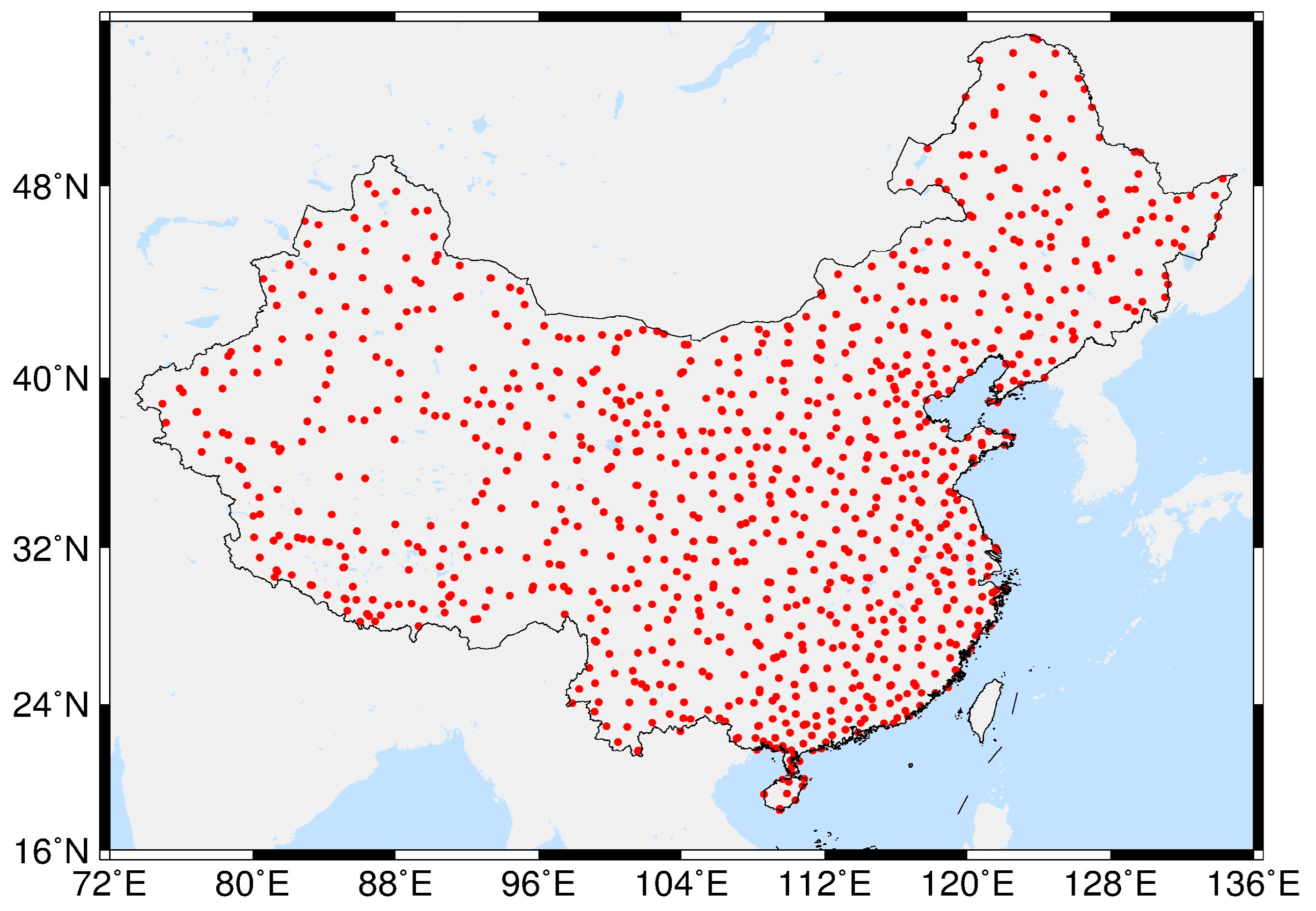
2.1.2. GNSS/Levelling Data

The GNSS/leveling observations of China are utilized for evaluating accuracy of GFMs. The high-accuracy first-order spirit levelling height are obtained, which is based on a Chinese 1985 vertical datum. The level origin with a normal height of 72.2604 m is located in Qingdao. The least square adjustment is utilized to eliminate accumulated systematic errors in long-distance leveling. In addition, to obtain normal height in adjustment, the correction for non-parallelism of level surface, solid-tide correction, gravity anomaly reduction, and ocean-tide loading correction are performed [41]. The mean square error of leveling per kilometer after adjustment is ±1 mm. Finally, the 984 GNSS/leveling benchmarks are utilized to verify the accuracy of GFMs. The GNSS ellipsoidal coordinates reach the millimeter accuracy level based on ITRF2014 [42]. Figure 1 represents the spatial location of the GNSS/leveling.

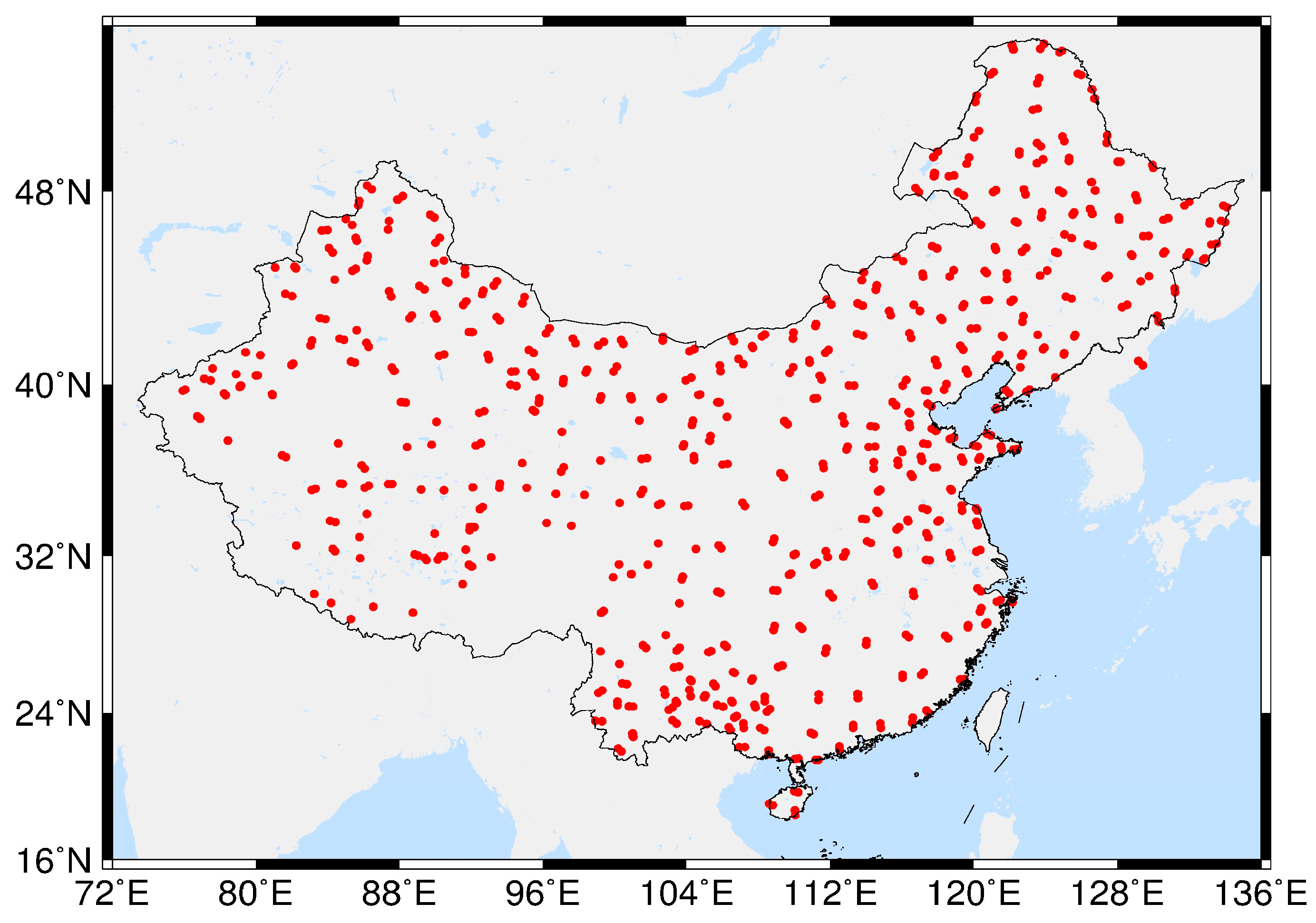
2.1.3. Deflection of the Vertical (DOV) Data

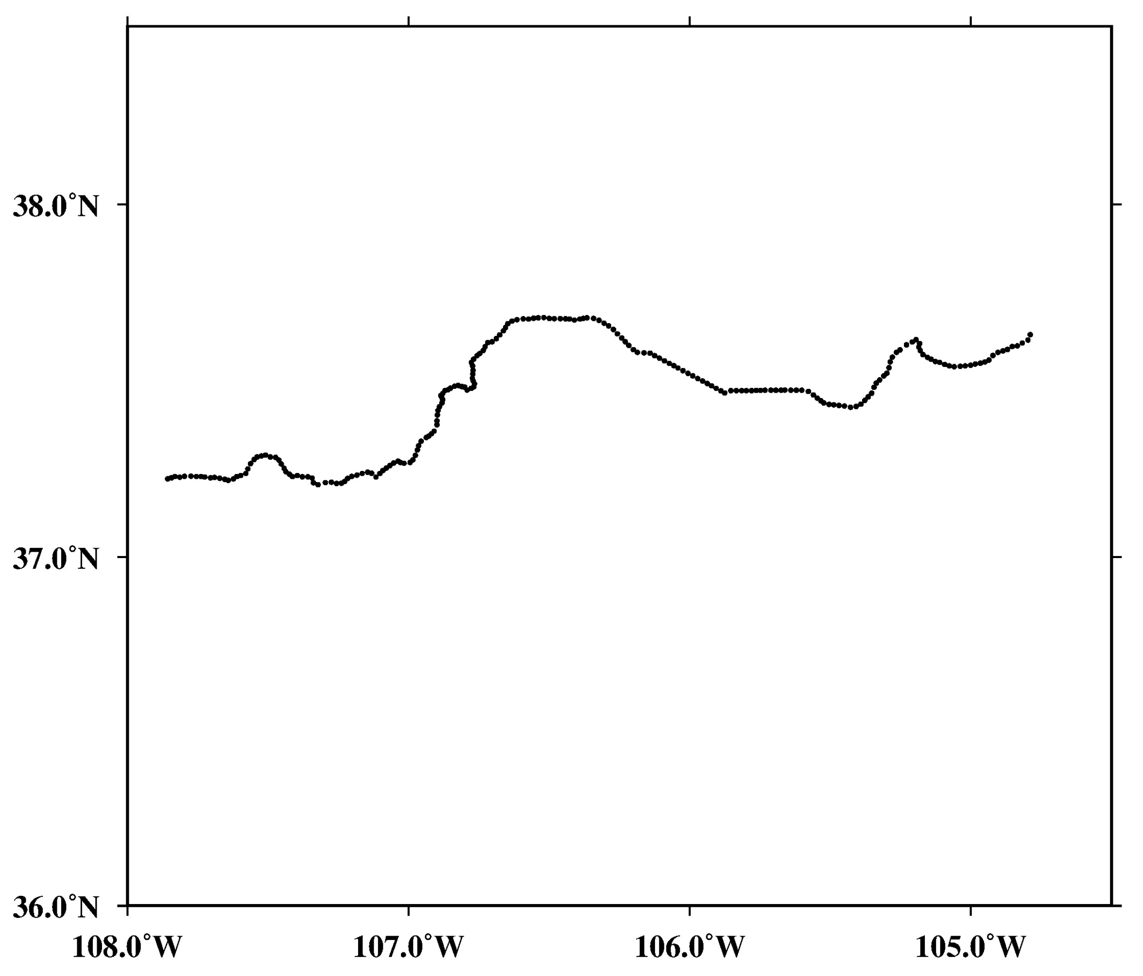
The DOV is also utilized to validate accuracy of the GFMs. Compared with the geoid height or height anomaly, the short wavelength spectrum power proportion of DOV has a larger increase [27], which can further reflect the high-frequency gravity field signal. There are two datasets of DOV data used in this study. The first group is 696 evenly distributed astronomical geodetic DOV data in mainland China, which has an accuracy level of ~0.14″. Figure 2 represents the spatial location of DOV data of mainland China. The second DOV dataset is from the Colorado geoid experiment [43], which has an accuracy level of ~0.04″ [38]. Figure 3 shows the survey line of DOV in Colorado, USA.

2.1.4. Gravity Data

To further validate the accuracy of the GFMs, the 1,835,358 evenly distributed gravity observations from Australia and 822,301 gravity observations from mainland America are used. The Australia gravity dataset is provided from the Geoscience Australia’s National Gravity Database, and the America gravity dataset is provided by the National Oceanic and Atmospheric Administration (NOAA). We can obtain the absolute gravity value of Earth surface from Geoscience Australia’s National Gravity Database and NOAA; then, we calculate normal gravity based on the GRS80 reference ellipsoid and apply free-air correction for deriving the gravity anomalies [44]. Finally, free-air gravity anomalies are obtained. Figure 4 and Figure 5 represent the distribution of gravity observations of Australia and mainland America, respectively.

2.2. Methodology

2.2.1. Method for Determining the Augmented Gravity Field Models

We can combine the topographic potential models and the EIGEN_6C4 model to obtain combined GFMs via the spectral expansion approach, which is to augment EIGIEN_6C4 model using topographic potential models (TPMs). In order to ensure the smooth transition of the combination of TPMs and high-degree GFMs [37], we set a certain transition zone, in which a Hanning function is used to combine EIGEN_6C4 with the corresponding degree of topographic potential models. Then, the degrees 0~N₁ of the refined GFM are the potential coefficient corresponding to the EIGEN_6C4 model, (N₂ + 1)~N_max (N_max is the maximum degree of the topographic potential models) is supplemented by degree corresponding to topographic potential models. The potential coefficients of transition zone (N₁~N₂₎ based on weighted combination can be expressed as

$$\left\{\begin{array}{l}{\overline{C}}_{nm}^{Combine}=P_1\cdot {\overline{C}}_{nm}^{EIGEN}+\left(1-P_1\right)\cdot {\overline{C}}_{nm}^{Topography}\\ {\overline{S}}_{nm}^{Combine}=P_1\cdot {\overline{S}}_{nm}^{EIGEN}+\left(1-P_1\right)\cdot {\overline{S}}_{nm}^{Topography}\end{array}\right.$$

(1)

where ${\overline{C}}_{nm}^{Combine}$ and ${\overline{S}}_n^{Combine}$ are the potential coefficients of transition zone, respectively, ${\overline{C}}_{nm}^{EIGEN}$ and ${\overline{S}}_{nm}^{EIGEN}$ are the potential coefficients of the EIGEN_6C4 model, respectively, ${\overline{C}}_{nm}^{Topography}$ and ${\overline{S}}_{nm}^{Topography}$ are the potential coefficients of topographic potential models, respectively, n and m are the degree and order, respectively, and P₁ represents weight. The weight P₁ can be determined by a Hanning function [11,45], which can be expressed by

$$P_1=\frac{1}{2}\left[1-cos\left(\frac{\pi \left(N-dN-n\right)}{2dN}\right)\right]$$

(2)

where N = (N₁ + N₂)/2 represents the central degree and dN = (N₂ − N₁)/2 is the half-bandwidth in transition zone.

The consistency of gravity field models geometric parameters should be considered when the topographic potential model is used to extend the EIGEN_6C4 model. Therefore, the geometric parameters are unified to the GRS80 reference ellipsoid before combination. The parameters are unified by the following equation [46]:

$$\left\{\begin{array}{l}{\overline{C}}_{nm}\\ {\overline{S}}_{nm}\end{array}\right\}=\frac{GM}{G{M}^{GRS80}}{\left(\frac{a}{a^{GRS80}}\right)}^n\left\{\begin{array}{l}{\overline{C}}_{{}_{nm}}^{GGM}\\ {\overline{S}}_{nm}^{GGM}\end{array}\right\}$$

(3)

where ${\overline{C}}_{nm}$ and ${\overline{S}}_{nm}$ are potential coefficients of the GFM after parameter conversion, ${\overline{C}}_{{}_{nm}}^{GGM}$ and ${\overline{S}}_{nm}^{GGM}$ are potential coefficients of the GFM before parameter conversion, GM = 3.986005000 × 10¹⁴ m³ s⁻² is the constants of gravitational constant the GRS80 ellipsoid [47], and a^GRS80 = 6,378,137.0 represents the semimajor axis of ellipsoid. The geometric parameters of the EIGEN_6C4, dV_ELL_Earth2014_5480, and ROLI_EllApprox_SphN_3660 models are shown in Table 1. The parameters of the dV_ELL_Earth2014_5480 model are consistent with the GRS80 ellipsoid. The parameters of EIGEN_6C4 and ROLI_EllApprox_SphN_3660 models can be unified by Equation (3).

Finally, the height anomaly $\zeta$, gravity anomaly $\Delta g$, the east–west component of the DOV $\eta$, and the south–north component of the DOV $\xi$ can be determined from the augmented gravity field models by [48]

$$\zeta =\frac{G{M}^{GRS80}}{\gamma \times r}{\displaystyle {\sum }_{n=2}^{N_{\max }}{\left(\frac{a^{GRS80}}{r}\right)}^n{\displaystyle {\sum }_{m=0}^n(\Delta {\overline{C}}_{nm}^{}cos m\lambda +{\overline{S}}_{nm}^{}sin m\lambda )}}{\overline{P}}_{nm}^{}\left(sin \phi \right)$$

(4)

$$\Delta g=\frac{G{M}^{GRS80}}{r^2}{\displaystyle {\sum }_{n=0}^{N_{\max }}{\left(\frac{a^{GRS80}}{r}\right)}^n\left(n-1\right){\displaystyle {\sum }_{m=0}^n(\Delta {\overline{C}}_{nm}^{}cos m\lambda +{\overline{S}}_{nm}^{}sin m\lambda )}}{\overline{P}}_{nm}^{}\left(sin \phi \right)$$

(5)

$$\xi =-\frac{G{M}^{GRS80}}{\gamma \times r^2}{\displaystyle {\sum }_{n=0}^{N_{\max }}{\left(\frac{a^{GRS80}}{r}\right)}^n{\displaystyle {\sum }_{m=0}^n(\Delta {\overline{C}}_{nm}^{}cos m\lambda +{\overline{S}}_{nm}^{}sin m\lambda )}}\frac{d{\overline{P}}_{nm}^{}\left(sin \phi \right)}{d\phi }$$

(6)

$$\eta =-\frac{G{M}^{GRS80}}{\gamma \times r^2\times cos \phi }{\displaystyle {\sum }_{n=0}^{N_{\max }}{\left(\frac{a^{GRS80}}{r}\right)}^n{\displaystyle {\sum }_{m=0}^n(-\Delta {\overline{C}}_{nm}^{}sin m\lambda +{\overline{S}}_{nm}^{}cos m\lambda )}}m{\overline{P}}_{nm}^{}\left(sin \phi \right)$$

(7)

where r is the geocentric radial of computation point, $\gamma$ is the normal gravity, and $\phi$ and $\lambda$ are the latitude and longitude of calculated point, respectively, $\Delta {\overline{C}}_{nm}^{}$ represents difference between even degree (2n, n = 0, 1, 2 …, 10) and order zero (m = 0) potential coefficients of the refined GFMs and the corresponding potential coefficients of normal gravitational potential. ${\overline{P}}_{nm}^{}\left(sin \phi \right)$ is the normalized associated Legendre function.

2.2.2. Spectral Evaluations of Gravity Field Models

The spectral characteristics of disturbing gravity field in various wavelengths can be represented by degree variances and cumulative degree variance, which can represent the signal power of GFM. This paper will calculate degree variance and cumulative degree variance to analyze spectral accuracy of the GFM. The degree variance and cumulative degree variance can be represented by the potential coefficients of the GFMs under spherical approximation, which can be expressed by [49,50]

$${\sigma }_{{}_n}^2=c^2\times {\displaystyle \sum _{m=0}^n\left[C_{nm}^2\left(c\right)+S_{nm}^2\left(s\right)\right]}$$

(8)

where ${\sigma }_{{}_n}^2$ represents the degree variance for GFM, $C_{{}_{nm}}^{}\left(c\right)$ and $S_{{}_{nm}}^{}\left(c\right)$ represent the spherical harmonic coefficient, and c represents the scale factor. We can choose different scale factors to represent spectral accuracy of different disturbing gravity field.

Table 2. Signal scale factor of function of disturbing gravity field.

Function	Factor	Unit
geoid	R	m
Gravity anomaly	$\frac{GM}{R^2}\times \left(n-1\right)\times {10}^5$	mGal
Gravity disturbance	$\frac{GM}{R^2}\times \left(n+1\right)\times {10}^5$	mGal
DOV	$180\times 3600/\pi \times (n^2+n)$	arcsec

shows the signal scale factors for disturbing gravity field.

The cumulative degree variance can be expressed by following equation:

$${\sigma }_{{}_{cum}}^2=c^2\times {\displaystyle \sum _{n=0}^{N_{max}}{\displaystyle \sum _{m=0}^n\left[C_{nm}^2\left(c\right)+S_{nm}^2\left(s\right)\right]}}$$

(9)

A relative comparison of the two models can be represented by the cumulative difference degree variance, which can be expressed by

$$\Delta {\sigma }_{{}_{cum}}^2=c^2\times {\displaystyle \sum _{n=0}^{N_{max}}{\displaystyle \sum _{m=0}^n\left[\Delta C_{nm}^2\left(c\right)+\Delta S_{nm}^2\left(s\right)\right]}}$$

(10)

where $\Delta {\sigma }_{{}_{cum}}^2$ is the cumulative difference degree variance and $\Delta C_{nm}^{}\left(c\right)$ and $\Delta S_{nm}^{}\left(s\right)$ represent the difference of model potential coefficients.

3. Results

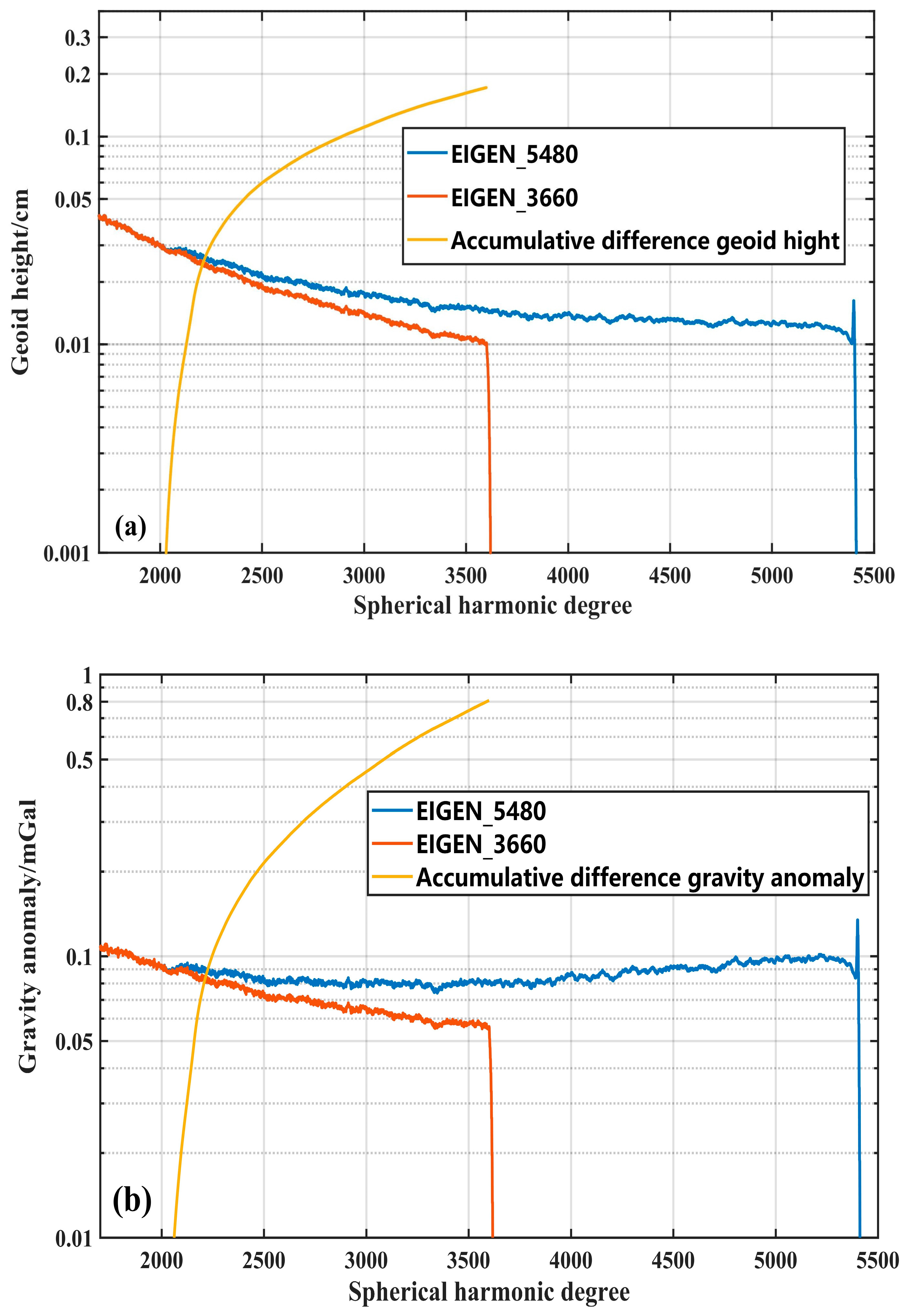
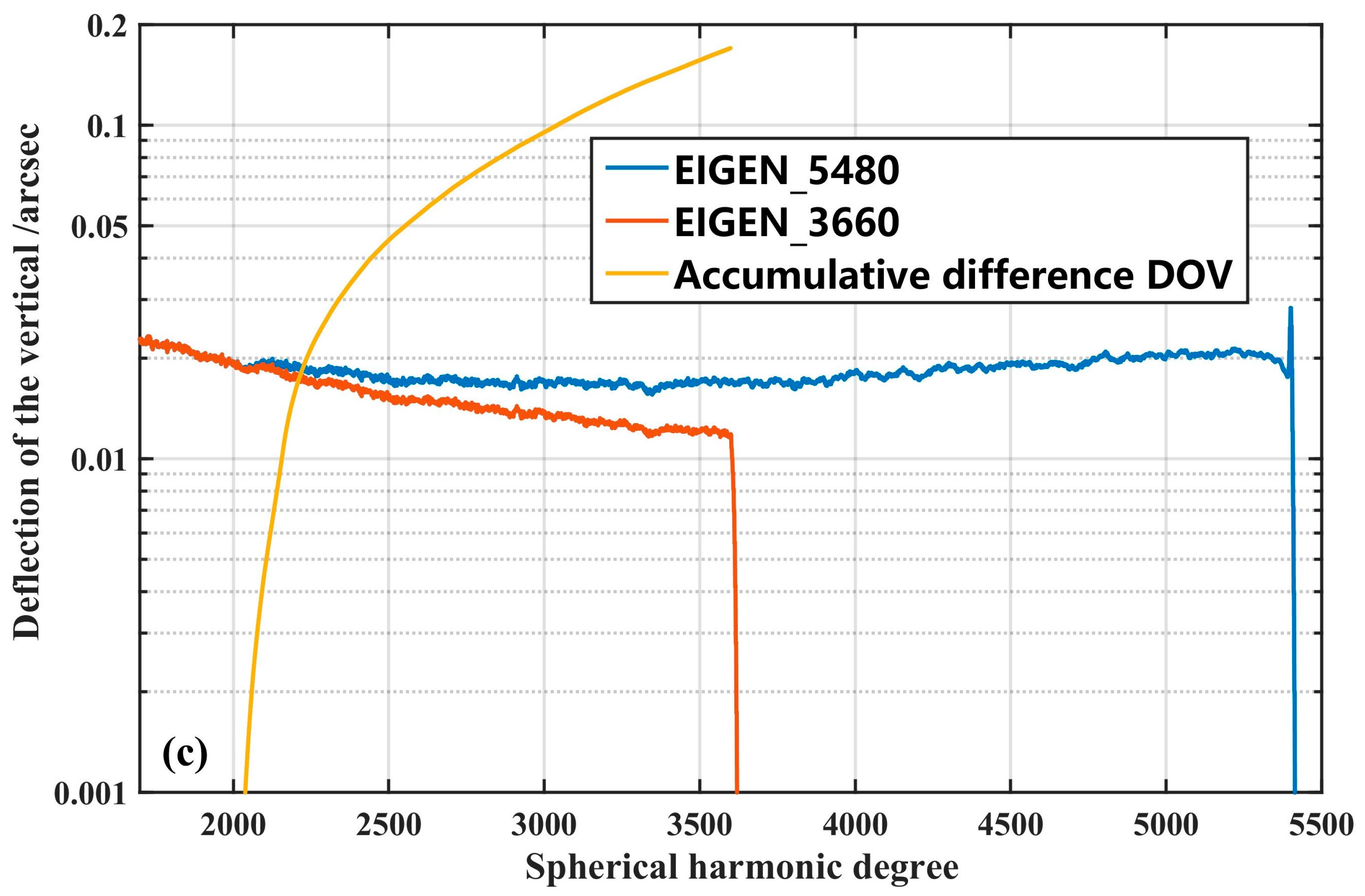
3.1. Spectral Accuracy Analysis of GFMs

The degree variance of GFMs is determined to evaluate spectral accuracy of GFM. Figure 6 shows the square root of degree variance in geoid height, gravity anomaly, and DOV of different GFM, respectively, which represents signal degree amplitudes of a disturbing gravity field. We can see from the figure that the signal degree amplitudes of dV_ELL_Earth2014_5480 and ROLI_EllApprox_SphN_3660 models before about degree 900 have a difference from EIGEN_6C4 model because the topographic potential models mainly reflect the gravity variation caused by the near-surface Earth mass. Therefore, the long wavelength gravity field signal cannot be well represented in topographic potential models. However, the higher-degree part of the topographic potential models can effectively represent high-frequency signals. In addition, the dV_ELL_Earth2014_5480 and ROLI_ EllApprox_SphN_3660 models have certain high-frequency geoid signal after degree 2190 compared to the EIGEN_6C4 model. The gravity field signals of dV_ELL_Earth2014_5480 and ROLI_ EllApprox_SphN_3660 models are basically consistent before about degree 2000, and there are some differences after about degree 2000. The dV_ELL_Earth2014_5480 model still has certain gravity field signal after degree 3660 compared to ROLI_EllApprox_SphN_3660 model. The dV_ELL_Earth2014_5480 model has a jump at about degree 5400, which is attributed to the characteristics of the spectral forward modelling technique at high spectral degree. From the above analysis, we can conclude that different gravity field models have different spectral characteristic. The higher-frequency signals in topographic potential models can be used to compensate for the high-frequency signal absence of GFMs of degree 2190.

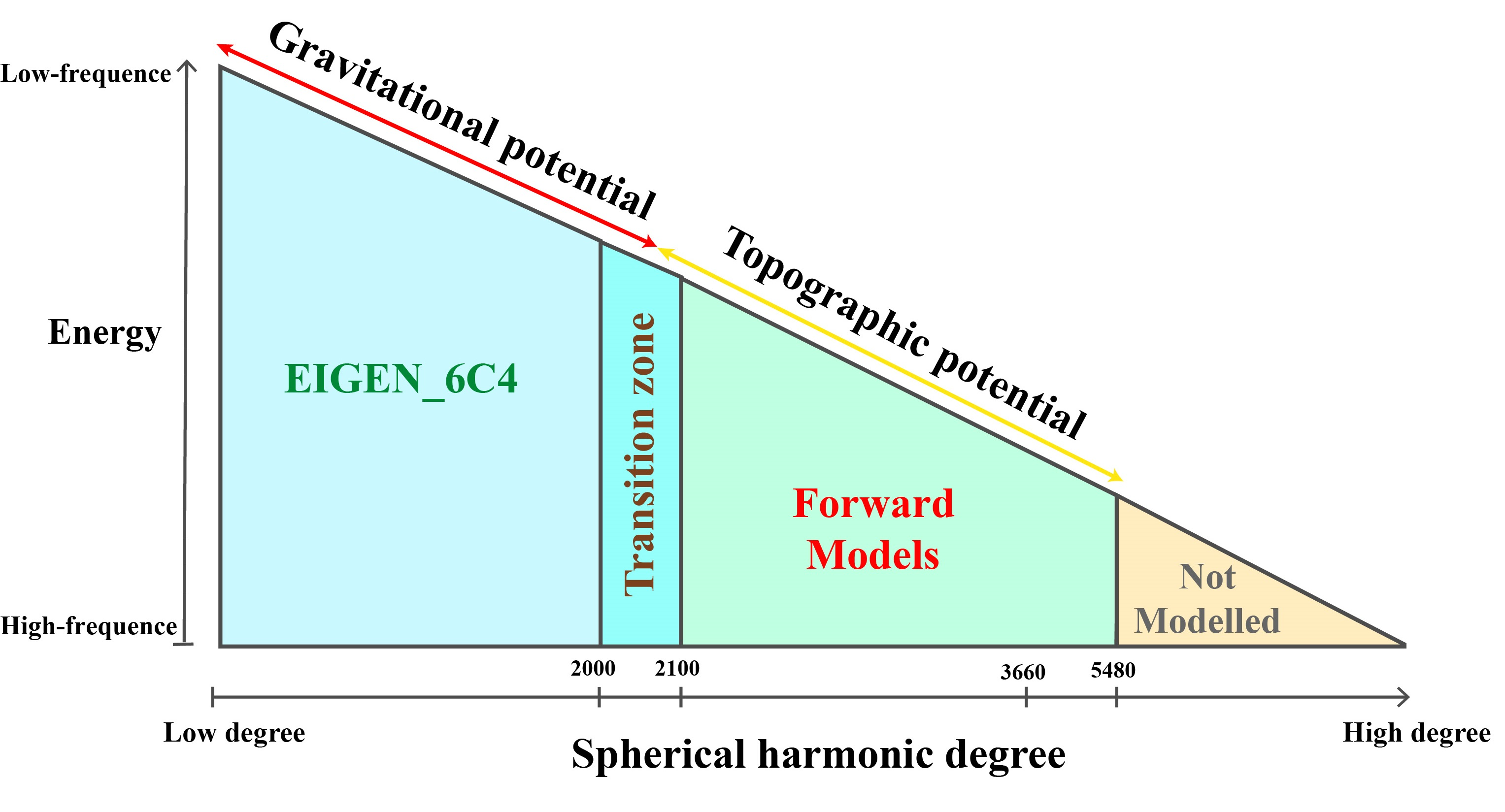
3.2. Construction of the Augmented GFMs

The dV_ELL_Earth2014_5480 and ROLI_EllApprox_SphN_3660 models are used to expand EIGEN_6C4 model for constructing refined GFMs. In order to ensure smooth transition of two GFMs during the combination, a certain transition zone is set to 2000–2100 [37], i.e., N₁ = 2000, N₂ = 2100; therefore, the central degree N is 2050 and half-bandwidth dN is 50. In the transition zone, a weighted method is used to combine EIGEN_6C4 with the topographic potential models. The degrees 0~2000 of the refined GFMs are the potential coefficient corresponding to the EIGEN_6C4 model; the degrees beyond 2100 are supplemented by the topographic potential models. Finally, the refined models EIGEN_3660 and EIGEN_5480 are determined.

Figure 7 shows the square root of geoid degree variance of EIGEN_6C4, EIGEN_3660, and EIGEN_5480 models. We can see from the figure that the geoid signal amplitudes of EIGEN_6C4 model are consistent with the EIGEN_3660 and EIGEN_5480 models before approximately degree 2000. This is due to the EIGEN_3660 and EIGEN_5480 models fully utilizing gravity field information of the EIGEN_6C4 model before degree 2000. The geoid signal of EIGEN_3660 and EIGEN_5480 is better than that of the EIGEN_6C4 model after degree 2000, which is due to the EIGEN_3660 and EIGEN_5480 models including the high frequency gravity field signal of the TPM. In addition, the geoid signal of the EIGEN_5480 model outperforms the EIGEN_3660 model after about degree 3660. Therefore, the EIGEN_6C4 model and topographic potential models can be combined to derive the combined models. The determined models can retain the low-frequency gravity field information of the EIGEN_6C4 and the high-frequency signal of the TPMs.

The higher-degree spectral characteristics of the refined GFMs are analyzed to further analyze the difference between EIGEN_3660 and EIGEN_5480 models. Figure 8 represents the signal amplitudes of the EIGEN_3660 and EIGEN_5480 models and the cumulative differences amplitude between both expanded models in terms of geoid height, gravity anomaly, and deflection of the vertical (DOV). We can see from the figure that the EIGEN_3660 and EIGEN_5480 models have some signal differences in terms of geoid height, gravity anomaly, and DOV from degree 2000 to 3660. Before about degree 3660, both expanded models have a geoid cumulative difference of ~1.8 cm, a gravity anomaly cumulative difference of ~0.8 mGal, and a deflection of the vertical cumulative difference of ~0.18″, which is caused by the spectral forward modelling strategy and method. The cumulative difference between both expanded models from degree 2000 to 3660 can be ignored considering that the spectral difference is the global average gravity field signal difference of the corresponding disturbing gravity field. After degree 3660, the signals of geoid, gravity anomaly, and DOV for the EIGEN_3660 model have disappeared; however, the EIGEN_5480 model has a certain gravity field signal from degree 3660 to 5480.

3.3. Accuracy Validation of the Augmented GFMs

To validate accuracy of the refined GFMs obtained in this study, the high-quality GNSS/levelling data, DOV data, and gravity observations are used.

3.3.1. Accuracy Validation by GNSS/Levelling Data

A total of 984 GNSS/levelling observations from China are utilized to validate accuracy of the refined models. In addition, the EIGEN_6C4 model is also verified as a comparison.

Table 3. Height anomalies difference statistics between observed values and the GFMs. Unit: m.

Models	Max	Min	Mean	STD
EIGEN_6C4	1.284	−1.274	−0.098	0.267
EIGEN_3660	1.285	−1.283	−0.088	0.261
EIGEN_5480	1.362	−1.286	−0.077	0.258

shows height anomaly differences statistics between the observed values and EIGEN_6C4, EIGEN_3660, and EIGEN_5480 models.

From Table 3, we can see that both expanded models have better accuracy in determining height anomalies than EIGEN_6C4 model. The accuracy of EIGEN_3660 for deriving height anomalies is improved by about 0.6 cm compared to the EIGEN_6C4 model. The EIGEN_5480 model has a higher accuracy in determining height anomaly compared to EIGEN_6C4 and EIGEN_3660 models, which is attributed to its higher resolution. The accuracy of EIGEN_5480 for obtaining height anomaly has increased by about 0.9 cm compared to EIGEN_6C4 model, and the improvement range is 3.4%. The aforementioned results verify the validity of the refined gravity field models derived in this study. Therefore, considering high-frequency signals can further improve accuracy for determining height anomaly, the accuracy improvement for EIGEN_5480 model is attributed to the high-frequency signal of the terrain, which compensates for the omission errors of the EIGEN_6C4 model and results in accuracy improvement for determining high-frequency signal.

However, we can find from the results that the refined gravity field models for determining height anomaly have a minor accuracy improvement, which is attributed to the fact that the spectral power proportion of height anomaly (or geoid height) is mainly concentrated in medium–long wavelengths and the spectral power proportion of short wavelengths is limited.

3.3.2. Accuracy Validation by Deflection of the Vertical (DOV) Data

The DOV of China and Colorado are also used to validate the accuracy of GFMs. Compared with geoid height or height anomaly, the short wavelength spectrum power proportion of deflection of the vertical (DOV) is larger, which is more sensitive to the high-frequency gravity field signal.

Table 4. DOV differences statistics between observations and t the gravity field models in China. Unit: arcsec.

Component of DOV	Models	Max	Min	Mean	RMS
The meridian component	EIGEN_6C4	17.371	−17.9465	−0.207	2.770
	EIGEN_3660	16.009	−21.213	−0.189	2.234
	EIGEN_5480	14.418	−14.671	−0.155	2.186
The prime vertical component	EIGEN_6C4	14.9158	−14.5742	0.188	2.823
	EIGEN_3660	19.6499	−14.4563	0.115	2.386
	EIGEN_5480	14.9582	−11.1469	0.121	2.171

shows statistics for DOV differences between observations and EIGEN_6C4, EIGEN_3660, and EIGEN_5480 models in China. We can find from the table that both expanded models have better accuracy in determining deflection of the vertical than the EIGEN_6C4 model. The accuracy of EIGEN_3660 for deriving the south-north component of DOV is improved by approximately 19.5% compared to EIGEN_6C4 model. The accuracy of EIGEN_5480 for deriving the south–north component of DOV is improved by about 21.1% compared to EIGEN_6C4 model. In addition, compared to EIGEN_6C4 model, the EIGEN_3660 model has an acccuracy improvement of 19.5% for deriving the east–west component of DOV, and the EIGEN_5480 model has an acccuracy improvement of 23.1% for deriving the east–west component of DOV.

Table 5. DOV differences statistics between observations and the gravity field models in Colorado. Unit: arcsec.

Component of DOV	Models	Max	Min	Mean	RMS
The meridian component	EIGEN_6C4	3.978	−4.680	0.331	1.31
	EIGEN_3660	4.222	−3.740	0.267	1.06
	EIGEN_5480	2.213	−3.951	0.076	0.94
The prime vertical component	EIGEN_6C4	5.532	−7.851	−0.124	1.62
	EIGEN_3660	3.525	−3.956	−0.057	1.18
	EIGEN_5480	4.944	−2.150	−0.0429	1.05

shows statistics for DOV differences between observations and EIGEN_6C4, EIGEN_3660, and EIGEN_5480 models in Colorado. It can be seen from the table that both expanded models also have better accuracy in determining deflection of the vertical than the EIGEN_6C4 model. The accuracy of EIGEN_3660 for deriving the south–north component of DOV is improved by approximately 19.1% compared to the EIGEN_6C4 model. The accuracy of EIGEN_5480 for deriving the south–north component of DOV is improved by about 28.2% compared to EIGEN_6C4 model. In addition, compared to the EIGEN_6C4 model, the EIGEN_3660 model has an acccuracy improvement of 27.2% for deriving the east–west component of DOV, and the EIGEN_5480 model has an acccuracy improvement of 35.2% for deriving the east–west component of DOV. The EIGEN_5480 model has a higher accuracy for determining DOV compared to the EIGEN_3660 model, which is attributed to its higher resolution. From the comparison results of the determined models for deriving the DOV in mainland China and Colorado, we can find that the accuracy improvement is larger in Colorado, because the Colorado region is mountainous and the terrain is rugged.

The above analysis indicates that the accuracy of the refined models for determining deflection of the vertical has been improved. The accuracy improvement of DOV determination is more obvious compared with height anomaly determination. Therefore, the refined gravity field models plays a well role in determining disturbing gravity field by introducing topographic gravity field signals.

3.3.3. Accuracy Validation by Gravity Data

The 1,835,358 evenly distributed gravity observations from Australia and 822,301 gravity observations from mainland America are used to further validate the accuracy of the determined models.

Table 6. Gravity anomalies differences statistics between observed gravity anomalies values and the gravity field models in Australia. Unit: mGal.

Models	Max	Min	Mean	RMS
EIGEN_6C4	72.40	−195.50	−0.45	4.79
EIGEN_3660	72.19	−192.95	−0.25	4.31
EIGEN_5480	87.30	−194.40	−0.19	4.00

and

Table 7. Gravity anomalies differences statistics between observed gravity anomalies values and the gravity field models in mainland America. Unit: mGal.

Models	Max	Min	Mean	RMS
EIGEN_6C4	155.37	−179.61	−0.67	10.49
EIGEN_3660	148.72	−157.28	−0.53	9.73
EIGEN_5480	128.16	−160.59	−0.15	9.30

represent difference statistics between observed gravity anomalies and EIGEN_6C4, EIGEN_3660, and EIGEN_5480 models in Australia and mainland America, respectively. We can conclude from the tables that both expanded models have better accuracy in determining gravity anomaly than the EIGEN_6C4 model. In Australia, the accuracy of EIGEN_3660 for deriving gravity anomaly is improved by about 10.05% compared to the EIGEN_6C4 model, and the accuracy of EIGEN_5480 for deriving gravity anomaly is improved by about 16.5% compared to the EIGEN_6C4 model. In mainland America, the accuracy of EIGEN_3660 for deriving gravity anomaly is improved by about 7.2% compared to the EIGEN_6C4 model. The accuracy of EIGEN_5480 for deriving gravity anomaly is improved by about 11.3% compared to the EIGEN_6C4 model. Among the two refined gravity field models, the EIGEN_5480 model has a greater accuracy improvement for gravity anomaly determination.

From the above analysis, it is also shown that the EIGEN_5480 and EIGEN_3660 models have a good accuracy improvement for determining disturbing gravity field, which also verifies the reliability of the determined models in this paper.

4. Discussion

From Figure 6, we can see from the figure that the signal powers of the topographic potential models have a difference from the EIGEN_6C4 model, which is because topographic potential models reflect the gravity variation caused by the near-surface Earth mass and the long wavelength g signal cannot be well represented. However, the higher-degree part of the topographic potential models contains high-frequency signals, which can be utilized for compensating the signal deficiency of GFMs of degree 2190. Therefore, combining the topographic potential models and EIGEN_6C4 model to derive refined gravity field models is a feasible mean. Numerical results of spectral characteristics analysis show that the determined EIGEN_3660 and EIGEN_5480 models can retain the low-frequency gravity field information of EIGEN_6C4 and the high-frequency signal of the TPMs. After about degree 2190, The signal degree amplitudes of geoid, gravity anomaly and DOV for the EIGEN_6C4 model have disappeared, and the EIGEN_5480 and EIGEN_3660 models have a certain gravity field signal. In addition, the EIGEN_3660 and EIGEN_5480 models have some signal differences in terms of geoid height, gravity anomaly, and DOV from degree 2000 to 3660; such differences may be caused by the spectral forward modeling strategy and method.

We combine the topographic potential models and EIGEN_6C4 model for deriving refined GFMs EIGEN_3660 and EIGEN_5480. The results presented in Figure 7 show that the geoid signal of EIGEN_3660 and EIGEN_5480 is better than that of the EIGEN_6C4 model after degree 2000, which is due to the EIGEN_3660 and EIGEN_5480 models including the high-frequency gravity field signal of the TPM. The determined GFMs can retain the low-frequency information of EIGEN_6C4 and the high-frequency signal of TPM. In addition, from Table 3, Table 4, Table 5, Table 6 and Table 7, we can see that the accuracy of the determined models for determining disturbing gravity field has been improved. The accuracy improvement of DOV and gravity anomaly determination is more obvious compared with height anomaly determination, which is attributed to the fact that the spectral power proportion of height anomaly (or geoid height) is mainly concentrated in medium–long wavelengths and the spectral power proportion of short wavelengths is limited. Therefore, the refined gravity field models play a significant role in determining disturbing gravity field by introducing topographic gravity field signals.

The refined gravity field models provide good accuracy for determining the disturbing gravity field. The validity has been verified by spectral accuracy evaluation and ground observations. However, the combination of the EIGEN_6C4 model with the TPMs is by a simple spherical harmonic coefficient combination, which may have a spectral gap between them. The simple spherical harmonic coefficient combination has differences from the normal equation combination. The normal equation combination will be further implemented to derive the high-resolution GFMs in the future. In addition, the maximum resolution of the TPMs used in this paper is 2′ (degree 5480); however, the unified topographic data of land and sea has reached resolution of 15″ and is developing towards resolution of 3”. With the continuous release of high-resolution terrain data, global density models, and improvement of spectral domain forward modelling techniques [37,38], higher-resolution topographic potential models can be derived in the future, which can further promote the accuracy and resolution of the determined models obtained by combining EIGEN_6C4 and topographic potential models.

5. Conclusions

In this paper, we investigate the feasibility of the determination of high-resolution GFMs by using topographic potential models to expand the EIGEN_6C4 model. Firstly, the spectral characteristics of EIGEN_6C4 and TPMs are analyzed. Then, the EIGEN_3660 and EIGEN_5480 models are determined by a weighted combination approach. Finally, the augmented gravity field models are verified by GNSS/leveling data in China, deflection of the vertical (DOV) data in China and Colorado, and gravity data from Australia and mainland America.

Numerical results of spectral characteristics analysis show that the dV_ELL_Earth2014_5480 and ROLI_EllApprox_SphN_3660 models have a stronger high-frequency signal power compared to the EIGEN_6C4 model. The determined GFMs can retain the low-frequency gravity field information of the EIGEN_6C4 and the high-frequency signal of the TPMs. After about degree 2190, the signal degree amplitudes of geoid, gravity anomaly, and DOV for the EIGEN_6C4 model have disappeared, and the EIGEN_5480 and EIGEN_3660 models have a certain gravity field signal. In addition, the EIGEN_3660 and EIGEN_5480 models have some signal differences in terms of geoid height, gravity anomaly, and DOV from degree 2000 to 3660; such differences may be caused by the spectral forward modelling modeling strategy and method. After degree 3660, the EIGEN_5480 model has a certain gravity field signal.

Moreover, the validation results by the GNSS/leveling, DOV, and gravity data show that the determined EIGEN_3660 and EIGEN_5480 models have better accuracy than the EIGEN_6C4 model in determination of height anomaly, DOV, and gravity anomaly, and the EIGEN_5480 model has optimal accuracy. The accuracy of EIGEN_5480 for obtaining height anomaly has increased by about 3.4%. Compared with EIGEN_6C4 model, the accuracy of EIGEN_5480 model in determining south–north and east–west components of the DOV in China has been improved by about 21.1% and 23.1%, respectively. In the mountainous area of Colorado, the accuracy of the EIGEN_5480 model in determining south–north and east–west components of DOV has been improved by about 28.2% and 35.2% compared to EIGEN_6C4 model, respectively. In addition, gravity value comparison results in Australia and mainland America indicate that the accuracy improvement of the EIGEN_5480 model for deriving gravity anomalies is 16.5% and 11.3% compared to the EIGEN_6C4 model, respectively.

References

1. Sánchez, L.; Ågren, J.; Huang, J.; Wang, Y.M.; Mäkinen, J.; Pail, R.; Barzaghi, R.; Vergos, G.S.; Ahlgren, K.; Liu, Q. Strategy for the realisation of the International Height Reference System (IHRS). J. Geod. 2021, 95, 33. [Google Scholar] [CrossRef]
2. Sánchez, L.; Sideris, M.G. Vertical datum unification for the International Height Reference System (IHRS). Geophys. J. Int. 2017, 209, 570–586. [Google Scholar] [CrossRef]
3. Zhang, P.; Li, Z.; Bao, L.; Zhang, P.; Wang, Y.; Wu, L.; Wang, Y. The Refined Gravity Field Models for Height System Unification in China. Remote Sens. 2022, 14, 1437. [Google Scholar] [CrossRef]
4. Sánchez, L.; Ågren, J.; Huang, J.; Wang, Y.M.; Mäkinen, J.; Denker, H.; Ihde, J.; Abd-Elmotaal, H.; Ahlgren, K.; Amos, M.; et al. Advances in the realisation of the International Height Reference System. In Proceedings of the IUGG General Assembly, Rio de Janeiro, Brazil, 12–14 November 2019. [Google Scholar]
5. Liu, H.; Wu, L.; Bao, L.; Li, Q.; Zhang, P.; Xi, M.; Wang, Y. Comprehensive Features Matching Algorithm for Gravity Aided Navigation. IEEE Geosci. Remote Sens. Lett. 2022, 19, 1–5. [Google Scholar] [CrossRef]
6. Zhang, P.; Wu, L.; Bao, L.; Wang, B.; Liu, H.; Li, Q.; Wang, Y. Gravity disturbance compensation for dual-axis rotary modulation inertial navigation system. Front. Mar. Sci. 2023, 10, 1086225. [Google Scholar] [CrossRef]
7. Zhang, P.; Bao, L.; Guo, D.; Wu, L.; Li, Q.; Liu, H.; Xue, Z.; Li, Z. Estimation of Vertical Datum Parameters Using the GBVP Approach Based on the Combined Global Geopotential Models. Remote Sens. 2020, 12, 4137. [Google Scholar] [CrossRef]
8. Zhang, P.; Bao, L.; Guo, D.; Li, Q. Estimation of the height datum geopotential value of Hong Kong using the combined global geopotential models and GNSS/levelling data. Surv. Rev. 2021, 54, 106–116. [Google Scholar] [CrossRef]
9. Tapley, B.D.; Bettadpur, S.; Watkins, M.; Reigber, C. The gravity recovery and climate experiment: Mission overview and early results. Geophy. Res. Lett. 2004, 31, L09607. [Google Scholar] [CrossRef] [Green Version]
10. Drinkwater, M.R.; Floberghagen, R.; Haagmans, R.; Muzi, D.; Popescu, A. GOCE: ESA’s first earth explorer core mission. In Earth Gravity Field from Space—From Sensors to Earth Science; Beutler, G., Ed.; Kluwer Academic Publishers: Bern, Switzerland, 2003; Volume 108, pp. 419–432. [Google Scholar]
11. Grombein, T.; Seitz, K.; Heck, B. On High-Frequency Topography-Implied Gravity Signals for a Height System Unification Using GOCE-based Global Geopotential Models. Surv. Geophys. 2016, 38, 443–477. [Google Scholar]
12. Gruber, T.; Visser, P.N.A.M.; Ackermann, C.; Hosse, M. Validation of GOCE gravity field models by means of orbit residuals and geoid comparisons. J. Geod. 2011, 85, 845–860. [Google Scholar] [CrossRef]
13. Hirt, C.; Gruber, T.; Featherstone, W.E. Evaluation of the first GOCE static gravity field models using terrestrial gravity, vertical defiections and EGM2008 quasigeoid heights. J. Geod. 2011, 85, 723–740. [Google Scholar] [CrossRef] [Green Version]
14. Tziavos, I.N.; Vergos, G.S.; Grigoriadis, V.N.; Tzanou, E.A.; Natsiopoulos, D.A. Validation of GOCE/GRACE Satellite Only and Combined Global Geopotential Models Over Greece in the Frame of the GOCESeaComb Project. In IAG 150 Years; Rizos, C., Willis, P., Eds.; Springer International Publishing: Cham, Switzerland, 2015; Volume 143, pp. 297–304. [Google Scholar]
15. Hirt, C.; Rexer, M.; Scheinert, M.; Pail, R.; Claessens, S.; Holmes, S. A new degree-2190 (10 km resolution) gravity field model for Antarctica developed from GRACE, GOCE and Bedmap2 data. J. Geod. 2016, 90, 105–127. [Google Scholar] [CrossRef]
16. Sandwell, D.T.; Mueller, R.D.; Smith, W.H.F.; Emmanuel, G.; Richard, F. Marine geophysics. New global marine gravity model from CryoSat-2 and Jason-1 reveals buried tectonic structure. Science 2014, 346, 65–67. [Google Scholar] [CrossRef] [PubMed]
17. Sandwell, D.T.; Harper, H.; Tozer, B.; Smith, W. Gravity Field Recovery from Geodetic Altimeter Missions. Adv. Space Res. 2019, 68, 1059–1072. [Google Scholar] [CrossRef]
18. Andersen, O.B.; Knudsen, P.; Berry, P.A.M. The DNSC08GRA global marine gravity field from double retracked satellite altimetry. J. Geod. 2010, 84, 191–199. [Google Scholar]
19. Pavlis, N.K.; Holmes, S.A.; Kenyon, S.C.; Factor, J.K. The development and evaluation of the earth gravitational model 2008(EGM2008). J. Geophys. Res. 2012, 117, B04406. [Google Scholar] [CrossRef] [Green Version]
20. Förste, C.; Bruinsma, S.L.; Abrykosov, O.; Lemoine, J.-M.; Marty, J.C.; Flechtner, F.; Balmino, G.; Barthelmes, F.; Biancale, R. EIGEN-6C4 the Latest Combined Global Gravity Field Model Including GOCE Data up to Degree and Order 2190 of GFZ Potsdam and GRGS Toulouse; GFZ Data Services: Potsdam, Germany, 2014. [Google Scholar]
21. Gilardoni, M.; Reguzzoni, M.; Sampietro, D. GECO: A global gravity model by locally combining GOCE data and EGM2008. Stud. Geophys. Geod. 2016, 60, 228–247. [Google Scholar] [CrossRef]
22. Liang, W.; Xu, X.; Li, J.; Zhu, G. The determination of an ultrahigh gravity field model SGG-UGM-1 by combining EGM2008 gravity anomaly and GOCE observation data. Acta Geod. Cartogr. Sin. 2018, 47, 425–434. [Google Scholar]
23. Liang, W.; Li, J.; Xu, X.; Zhang, S.; Zhao, Y. A High-Resolution Earth’s Gravity Field Model SGG-UGM-2 from GOCE, GRACE, Satellite Altimetry, and EGM2008. Engineering 2020, 6, 860–878. [Google Scholar]
24. Zingerle, P.; Pail, R.; Gruber, T.; Oikonomidou, X. The combined global gravity field model XGM2019e. J. Geod. 2020, 94, 66. [Google Scholar] [CrossRef]
25. Kaula, W.M. Theory of Satellite Geodesy; Blaisdell: Toronto, OH, USA, 1966. [Google Scholar]
26. Forsberg, R. Modelling of the fine-structure of the geoid: Methods, data requirements and some results. Surv. Geophys. 1993, 14, 403–418. [Google Scholar]
27. Denker, H. Regional Gravity Field Modeling: Theory and Practical Results. In Sciences of Geodesy—II Innovations and Future Developments; Xu, G., Ed.; Springer: Berlin/Heidelberg, Germany, 2013; pp. 185–291. [Google Scholar]
28. Tscherning, C.C.; Rapp, R.H. Closed Covariance Expressions for Gravity Anomalies, Geoid Undulations, and Deflections of the Vertical Implied by Anomaly Degree Variance Models; Reports of the Department of Geodetic Science; The Ohio State University: Columbus, OH, USA, 1974. [Google Scholar]
29. Hirt, C.; Claessens, S.; Fecher, T.; Kuhn, M.; Pail, R.; Rexer, M. New ultrahigh-resolution picture of earth’s gravity field. Geophy. Res. Lett. 2013, 40, 4279–4283. [Google Scholar] [CrossRef] [Green Version]
30. Yang, M.; Hirt, C.; Rexer, M.; Pail, P.; Yamazaki, D. The tree canopy effect in gravity forward modelling. Geophys. J. Int. 2019, 219, 271–289. [Google Scholar] [CrossRef]
31. Hirt, C.; Kuhn, M.; Claessens, S.; Pail, R.; Gruber, T. Study of the Earth short-scale gravity field using the ERTM2160 gravity model. Comput. Geosci. 2014, 73, 71–80. [Google Scholar] [CrossRef] [Green Version]
32. Hirt, C.; Yang, M.; Kuhn, M.; Bucha, B.; Kurzmann, A.; Pail, R. SRTM2gravity: An ultrahigh resolution global model of gravimetric terrain corrections. Geophys. Res. Lett. 2019, 46, 4618–4627. [Google Scholar] [CrossRef] [Green Version]
33. Rexer, M.; Hirt, C. Ultra-high degree surface spherical harmonic analysis using the Gauss-Legendre and the Driscoll/Healy quadrature theorem and application to planetary topography models of Earth, Moon and Mars. Surv. Geophys. 2015, 36, 803–830. [Google Scholar] [CrossRef]
34. Tozer, B.; Sandwell, D.T.; Smith, W.H.F.; Olson, C.; Beale, J.R.; Wessel, P. Global Bathymetry and Topography at 15 Arc Sec: SRTM15+. Earth Space Sci. 2019, 6, 1847–1864. [Google Scholar] [CrossRef]
35. Rexer, M.; Hirt, C.; Pail, R. High-Resolution Global Forward Modelling—A Degree-5480 Global Ellipsoidal Topographic Potential Model; EGU General Assembly, European Geosciences: Vienna, Austria, 2017. [Google Scholar]
36. Abrykosov, O.; Ince, E.S.; Foerste, C.; Flechtner, F. Rock-Ocean-Lake-Ice Topographic Gravity Field Model (ROLI Model) Expanded up to Degree 3660; GFZ Data Services: Potsdam, Germany, 2019. [Google Scholar]
37. Ince, E.S.; Abrykosov, O.; Förste, C.; Frank, F. Forward Gravity Modelling to Augment High-Resolution Combined Gravity Field Models. Surv. Geophys. 2020, 41, 767–804. [Google Scholar] [CrossRef] [Green Version]
38. Ince, E.S.; Förste, C.; Abrykosov, O.; Flechtner, F. Topographic Gravity Field Modelling for Improving High-Resolution Global Gravity Field Models. In International Association of Geodesy Symposia; Freymueller, J.T., Sánchez, L., Eds.; Springer International Publishing: Cham, Switzerland; Berlin/Heidelberg, Germany, 2022; Volume 154, pp. 1–10. [Google Scholar]
39. Huang, J.; Véronneau, M.; Crowley, J.W.; D’Aoust, B.; Pavlic, G. Can an Earth Gravitational Model Augmented by a Topographic Gravity Field Model Realize the International Height Reference System Accurately? In International Association of Geodesy Symposia; Freymueller, J.T., Sánchez, L., Eds.; Springer International Publishing: Cham, Switzerland; Berlin/Heidelberg, Germany, 2022; Volume 154, pp. 1–7. [Google Scholar]
40. Hirt, C.; Rexer, M. Earth2014: 1 arc-min shape, topography, bedrock and ice-sheet models—Available as gridded data and degree-10,800 spherical harmonics. Int. J. Appl. Earth Obs. Geoinf. 2015, 39, 103–112. [Google Scholar]
41. Wang, W.; Guo, C.; Li, D.; Zhao, H. Elevation change analysis of the national first order leveling points in recent 20 years. Acta Geod. Cartogr. Sin. 2019, 48, 1–8. [Google Scholar]
42. Altamimi, Z.; Rebischung, P.; Métivier, L.; Collilieux, X. ITRF2014: A new release of the International Terrestrial Reference Frame modeling nonlinear station motions. J. Geophys. Res. Solid Earth 2016, 121, 6109–6131. [Google Scholar] [CrossRef] [Green Version]
43. van Westrum, D.; Ahlgren, K.; Hirt, C.; Guillaume, S. A Geoid Slope Validation Survey (2017) in the rugged terrain of Colorado, USA. J. Geod. 2021, 95, 9. [Google Scholar] [CrossRef]
44. Hofmann-Wellenhof, B.; Moritz, H. Physical Geodesy; Springer: Wien, WI, USA, 2006. [Google Scholar]
45. Blackman, R.B.; Tukey, J.W. The measurement of power spectra from the point of view of communications engineering—Part I. Bell Syst. Tech. J. 1958, 37, 185–282. [Google Scholar]
46. He, L.; Li, J.; Chu, Y. Evaluation of the Geopotential Value for the Local Vertical Datum of China Using GRACE/GOCE GGMs and GPS/Leveling Data. Acta Geod. Cartogr. Sin. 2017, 46, 9. [Google Scholar]
47. Moritz, H. Geodetic reference system 1980. J. Geod. 2000, 74, 128–133. [Google Scholar]
48. Bucha, B.; Janák, J. A MATLAB-based graphical user interface program for computing functionals of the geopotential up to ultra-high degrees and orders. Comput. Geosci. 2013, 56, 186–196. [Google Scholar] [CrossRef]
49. Ustun, A.; Abbak, R. On global and regional spectral evaluation of global geopotential models. J. Geophys. Eng. 2010, 7, 369. [Google Scholar] [CrossRef]
50. Kelly, C.I.; Andam-Akorful, S.A.; Hancock, C.; Laari, P.; Ayer, J. Global gravity models and the Ghanaian Vertical Datum: Challenges of a proper definition. Surv. Rev. 2019, 53, 44–54. [Google Scholar]
51. Ince, E.S.; Barthelmes, F.; Reissland, S.; Elger, K.; Förste, C.; Flechtner, F.; Schuh, H. ICGEM—15 years of successful collection and distribution of global gravitational models, associated services, and future plans. Earth Syst. Sci. Data 2019, 11, 647–674. [Google Scholar] [CrossRef] [Green Version]
Figure 1. Spatial location of GNSS/leveling observations in mainland China.
Remotesensing 15 03418 g001
Figure 2. Spatial location of DOV benchmarks in China.
Remotesensing 15 03418 g002
Figure 3. Survey line of DOV data in Colorado, USA.
Remotesensing 15 03418 g003
Figure 4. The free-air gravity anomalies in Australia.
Remotesensing 15 03418 g004
Figure 5. The free-air gravity anomalies in America.
Remotesensing 15 03418 g005
Figure 6. Signal power of the GFMs in terms of (a) geoid height, (b) gravity anomaly and (c) DOV.
Remotesensing 15 03418 g006aRemotesensing 15 03418 g006b
Figure 7. The geoid signal power of the three models.
Remotesensing 15 03418 g007
Figure 8. The signal power of the expanded models EIGEN_3660 and EIGEN_5480 and the cumulative differences amplitude between both expanded models in terms of (a) geoid height, (b) gravity anomaly, and (c) deflection of the vertical (DOV).
Remotesensing 15 03418 g008aRemotesensing 15 03418 g008b