Article

Bi-Objective Crop Mapping from Sentinel-2 Images Based on Multiple Deep Learning Networks

1
Collaborative Innovation Center on Forecast and Evaluation of Metcorological Disasters, Nanjing University of Information Science & Technology (NUIST), Nanjing 210044, China
2
China Meteorological Administration Key Laboratory for Climate Prediction Studies, National Climate Center, Beijing 100081, China
3
School of Remote Sensing & Geomatics Engineering, Nanjing University of Information Science & Technology (NUIST), Nanjing 210044, China
4
School of Civil and Environmental Engineering, University of New South Wales (UNSW), Sydney 2052, Australia
*
Author to whom correspondence should be addressed.
Remote Sens. 2023, 15(13), 3417; https://doi.org/10.3390/rs15133417
Submission received: 1 June 2023 / Revised: 3 July 2023 / Accepted: 3 July 2023 / Published: 6 July 2023

Abstract

:
Accurate assessment of the extent of crop distribution and mapping different crop types are essential for monitoring and managing modern agriculture. Medium and high spatial resolution remote sensing (RS) for Earth observation and deep learning (DL) constitute one of the most major and effective tools for crop mapping. In this study, we used high-resolution Sentinel-2 imagery from Google Earth Engine (GEE) to map paddy rice and winter wheat in the Bengbu city of Anhui Province, China. We compared the performance of different popular DL backbone networks with the traditional machine learning (ML) methods, including HRNet, MobileNet, Xception, and Swin Transformer, within the improved DeepLabv3+ architecture, Segformer and random forest (RF). The results showed that the Segformer based on the combination of the Transformer architecture encoder and the lightweight multilayer perceptron (MLP) decoder achieved an overall accuracy (OA) value of 91.06%, a mean F1 Score (mF1) value of 89.26% and a mean Intersection over Union (mIoU) value of 80.70%. The Segformer outperformed other DL methods by combining the results of multiple evaluation metrics. Except for Swin Transformer, which was slightly lower than RF in OA, all DL methods significantly outperformed RF methods in accuracy for the main mapping objects, with mIoU improving by about 13.5~26%. The predicted images of paddy rice and winter wheat from the Segformer were characterized by high mapping accuracy, clear field edges, distinct detail features and a low false classification rate. Consequently, DL is an efficient option for fast and accurate mapping of paddy rice and winter wheat based on RS imagery.

1. Introduction

Paddy rice and wheat are the main food crops of China and the world, as well as commercial and strategic grain reserves [1,2], which have a major impact on human society and the natural environment [3]. There are winter and spring wheat in China, and winter wheat accounts for 98% [4]. Accurate mapping of paddy rice and winter wheat, especially during the growing seasons, is of great importance for maintaining food security and supporting the formulation of agricultural policies [5]. Traditional mapping of paddy rice and winter wheat requires many field surveys, which consumes considerable time and human resources with, however, low data quality [6].
The rapid development of remote sensing (RS) technology has provided an effective means of mapping crops in a fast, accurate and timely manner [7,8]. Currently, crop mapping is mainly based on the spectral reflectance in satellite images and vegetation phenology indicated by the temporal changes of vegetation indices (NDVI, EVI, etc.). Jiang et al. [9] analyzed the changes in paddy rice cropping systems in southern China based on the spectral characteristics of Landsat imagery. Dong et al. [10] proposed a new spectral similarity method for identifying winter wheat using Sentinel 2A/B image sequences, called phenology-time weighted dynamic time warping, which considers the phenological characteristics of winter wheat. Li et al. [4] presented a spectral reconstruction method based on singular value decomposition for winter wheat mapping, improving the spectral reference curves and, thus, the mapping results. Han et al. [11] combined MODIS and Sentinel-1 satellite data to produce a 10 m resolution paddy rice map of Southeast Northeast Asia from 2017 to 2019, based on the paddy rice transplanting flood signal land surface water index and paddy rice phenology determined from the backscatter coefficient changes. However, all these studies focus on a single paddy rice or winter wheat as the main object of study; however, it is not effective to separate different crops in areas with a complex cropping structure using only spectral properties or crop phenology [12]. The rice-wheat rotation (RWR) system is one of the oldest and most common agricultural practices in the Asian monsoon region, with about 130,000 km2 of land used for RWR in China [13] every year. The Yangtze-Huaihe economic zone is the main growing area for paddy rice and winter wheat in China and the main RWR area in the eastern part of the country [14]. Identifying multiple crops simultaneously in specific regions with complex cropping systems, such as East China, is still challenging.
In recent years, multiscale satellite observations have been fed into machine learning (ML) models such as decision trees (DTs), random forests (RFs), support vector machines (SVMs), and multilayer perceptrons (MLPs) [15,16,17,18,19]. ML models were initially designed to work with non-temporal, high-dimensional data rather than remotely sensed imagery with complex semantic features [20]. Today, many ML algorithms are being applied to satellite imagery to identify multiple crops, as spectral or textural features of multiple crops can be input into the classifiers [21]. Saini and Ghosh [22] used the extreme gradient boosting (XGBoost) method to address the similarity of crop spectra in Sentinel-2A images, achieving better performance than RF [23] and support vector machine methods in multi-crops mapping. Prins and Van Niekerk [24] used multiple classifiers to classify crops, finding that XGBoost and RF classifiers have the highest classification accuracy.
Deep learning (DL) is a branch of ML widely used in earth sciences, particularly in land cover classification and target identification [25]. It stands out in the RS field because it can clearly distinguish the spectral and spatial features of the original images. Compared to the traditional spectral, phonologic and ML methods, DL is characterized by the ability to accommodate large sample sizes without the need for pre-defined task-specific rules [26]. Most studies have constructed deep neural network (DNN) models for specific crop identification and classification problems, achieving satisfactory results compared to traditional spectroscopy and ML methods. Kussul et al. [27] found that the convolutional neural networks (CNNs) outperformed traditional fully connected lightweight MLP architecture for identifying crops in Ukrainian regions. Marcos et al. [28] propose a CNN architecture called Rotating Equivariant Vector Field Network for encoding the rotating equivariance of the network itself, showing better performance in crop mapping than the standard CNNs while requiring an order of magnitude fewer parameters.
The advent of AlexNet [29] established the dominance of CNNs in computer vision (CV), and since then CNNs have sprung up. As the performance of devices improved, some networks with deeper layers were introduced to the segmentation task. There seems to be a trend towards networks with deeper layers and more complex structures with more parameters [30], making some CNNs inapplicable on computationally limited platforms. MobileNet [31], on the other hand, is a model for mobile and embedded vision applications. The model is based on a streamlined architecture that uses deeply separable convolutions to build lightweight DNNs [31]. The Inception [32] model also emerged to reduce the number of network parameters and to obtain different receptive fields. It can divide the channel into several channels with different receptive field sizes. Chollet [33] explored the relationship between Inception and deep separable convolution from the perspective of the original Inception model, explained deep separable convolution from a new perspective, and proposed a new architecture inspired by the Inception module, Xception [33]. However, most current mainstream semantic segmentation (SS) networks are based on encoder-decoder structures [34]. Most segmentation networks based on encoder-decoder structures suffer from losing spatial information during the coding process [35]. To overcome these limitations, other advanced parallel structures have been proposed that extract low-resolution features while preserving high-resolution features throughout the network [36,37]. For example, in HRNet [38], information fragments in parallel multi-resolution subnetworks are repeatedly exchanged for multiscale fusion. This multi-scale fusion allows for an extended high-resolution representation. This simple modification improves the network’s performance and shows better results in vision tasks [39]. The Transformer [40] network structure has achieved far better results than other models in natural language processing (NLP) because it is based entirely on the attention mechanism and does not require recursive and convolutional structures. Dosovitskiy et al. [41] tried to separate attention from convolution and apply the pure Transformer directly to a sequence of patches formed by image splitting; the resulting Vision Transformer (ViT) achieves excellent image recognition results and a significant reduction in computational resources compared to advanced convolutional networks. To compensate for the shortcomings of ViT for visual tasks such as detection and segmentation, Liu et al. [42] proposed a new visual transformer called Swin Transformer, which can address the two major differences between visual entities that vary significantly in scale and images with generally higher pixel resolution than text. And to avoid the overly complex structure of SS models while maintaining the efficiency and performance of the model operation. Xie, et al. [43] proposed the Segformer model, which achieved excellent results on segmented datasets and showed strong zero-shot robustness. However, less research has been done to apply it to the SS of RS images. Nowadays, there are emerging DL algorithms for crop mapping from satellite images, and it is somewhat necessary to compare their performances in simultaneously mapping multiple crops [44]. However, there have been fewer studies on multi-crop classification using DL methods with paddy rice and winter wheat as the subjects.
The purpose of this study is to apply multiple DL SS networks to bi-objective crop mapping from Sentinel-2 Multispectral Instrument (MSI) Level 2A images in the Bengbu region of eastern China, where paddy rice and winter wheat are major food crops. The used networks include the high-resolution (HRNet) [45], MobileNet, Xception, Swin Transformer, Segformer and RF. Lastly, we contrast the results of each DL network with those of RF to assess the combined results of the different methods qualitatively and quantitatively on bi-objective mapping. The network with the best results could be selected as a methodological guide for related studies.

2. Materials and Methods
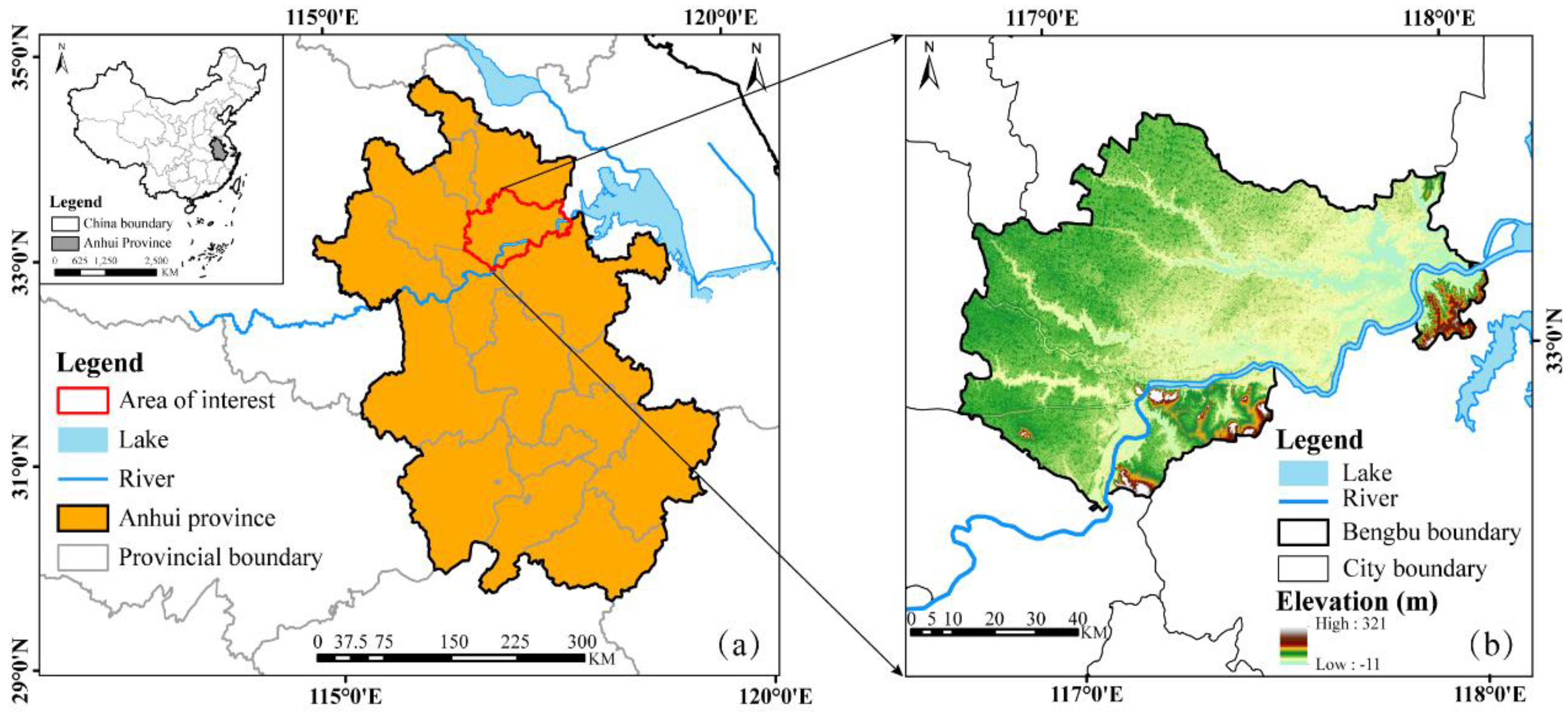
2.1. Study Area

As shown in Figure 1, Bengbu (32°43′N–33°30′N and 116°45′E–118°04′E) is located in the northern part of Anhui Province and is a prefecture-level city under the jurisdiction of Anhui Province. Geographically, Bengbu borders Jiangsu Province and Hongze Lake to the east, and the Qinling-Huaihe line (the geographical boundary between the north and the south of China) runs through the city of Bengbu. Bengbu has a flat terrain with a mainly plain landscape; hills are scattered in the south, with southeast-facing slopes from the northwest. Bengbu is located in the transition zone between the northern subtropical humid monsoon climate zone and the southern temperate semi-humid monsoon climate zone, with an average annual temperature of 15.5 °C and annual precipitation of about 905.4 mm. The monsoon climate is remarkable, with four distinct seasons, sufficient light, moderate temperature and precipitation, and climatic conditions that meet the climatic requirements for the growth of most crops [46]. According to the 2021 statistical bulletin on the national economic and social development of Bengbu City, released by the Statistical Bureau of Anhui Province, Bengbu City had an annual grain crop cultivation area of 5146.87 km2, of which 2511.69 km2 were winter wheat and 1056.47 km2 was paddy rice. Paddy rice is mostly single-season medium paddy rice, generally sown in April to May and matured for harvesting during the National Day; wheat is winter wheat, generally sown in October and matured for harvesting in June of the following year.

2.2. Data

2.2.1. Sentinel-2 Imagery

Sentinel-2 is a high-resolution multispectral imaging satellite under the European Space Agency’s Copernicus Programme, consisting of two satellites (2A and 2B), launched in June 2015 and March 2017, respectively. Its spatial resolutions are 10m (visible and NIR), 20 m (red edge and SWIR) and 60m (atmospheric bands), respectively. Sentinel-2 imageries are suitable for terrestrial monitoring, including vegetation, soil and water cover, inland waterways, coastal areas, and emergency relief services.
In this study, we utilize atmospherically and geometrically corrected low-level atmospheric reflectance Sentinel-2 Level-2A (L2A) product data from Google Earth Engine (GEE) for large area classification of multiple crops without additional data pre-processing. Sentinel-2 L2A data (2019 and later) are available from the GEE platform (https://developers.google.com/earth-engine/datasets/catalog/sentinel-2, accessed on 20 March 2022). 2018 L2A products were produced via the Sen2Cor plug-in. Based on this, we selected images for feature extraction of paddy rice and winter wheat from April 2018 to 2021. Sentinel-2’s QA60 band images with less than 10% clouds are selected by filtering with the de-clouding function; a median extraction operation is then used to obtain images that meet the conditions.

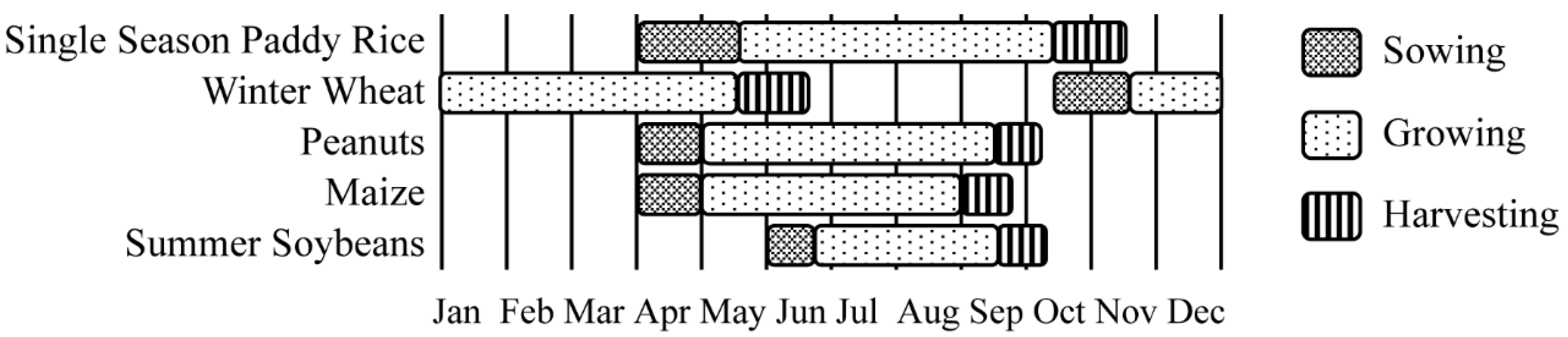
2.2.2. Crops Phenology Information

Phenology refers to the periodic changes with a certain pattern formed by organisms under the influence of various external environmental conditions, such as temperature and humidity, over a long period. Different crops usually have different phenological information, and the same crop has different phenological information in different regions [6]. From Xu and Fu [47], we obtained information on the main crops and their phenology in the study area. Figure 2 shows the main crop phenological information in Bengbu, where paddy rice (mostly single-season medium paddy rice), winter wheat, peanut, corn, and summer soybean are mainly cultivated. Among them, paddy rice and winter wheat are roughly complementary in terms of phenological timing, but there is a period of overlap in April and May each year. The spatial distribution of crop cultivation in Bengbu is relatively stable, with a few cases of crop rotation in a certain field, making this study feasible to a certain degree. This study selected the paddy rice sowing and germination period and the winter wheat tasseling period, i.e., late March to early May, for screening RS images generating training and test samples.

2.2.3. Production of Auxiliary Reference

Paddy rice and winter wheat have similar spectral features at specific periods, making it impossible to use manual visual interpretation to distinguish the two crops. Therefore, we set the corresponding normalized difference vegetation index (NDVI) thresholds for the classification masks of the two crops by the temporal variation of NDVI values in different phenological periods of paddy rice and winter wheat, such as the sowing, transplanting, tasseling, maturing, and harvesting periods. The mask is added to the RS image layer as a secondary reference for subsequent labeling.

2.3. Methods

This study compares the performance of CNN- and Transformer-based models—HRNet, MobileNet, Xception, Swin Transformer and Segformer—and the RF model in classifying Bengbu’s paddy rice and winter wheat. Figure 3 describes the main workflow of this study, including data acquisition and processing, model training and result comparison. We use DeepLabv3+ (the most representative architecture in SS tasks) as the main framework for embedding the four CNNs and the Swin Transformer. Also, the Segformer is used as another Transformer model representative and the traditional decision tree classifier, the RF, as a method compared to DL methods. The codes used in this study can be obtained online at https://github.com/tensorflow/models/tree/master/research/deeplab, (accessed on 1 August 2022) and https://github.com/NVlabs/SegFormer (accessed on 10 November 2022).

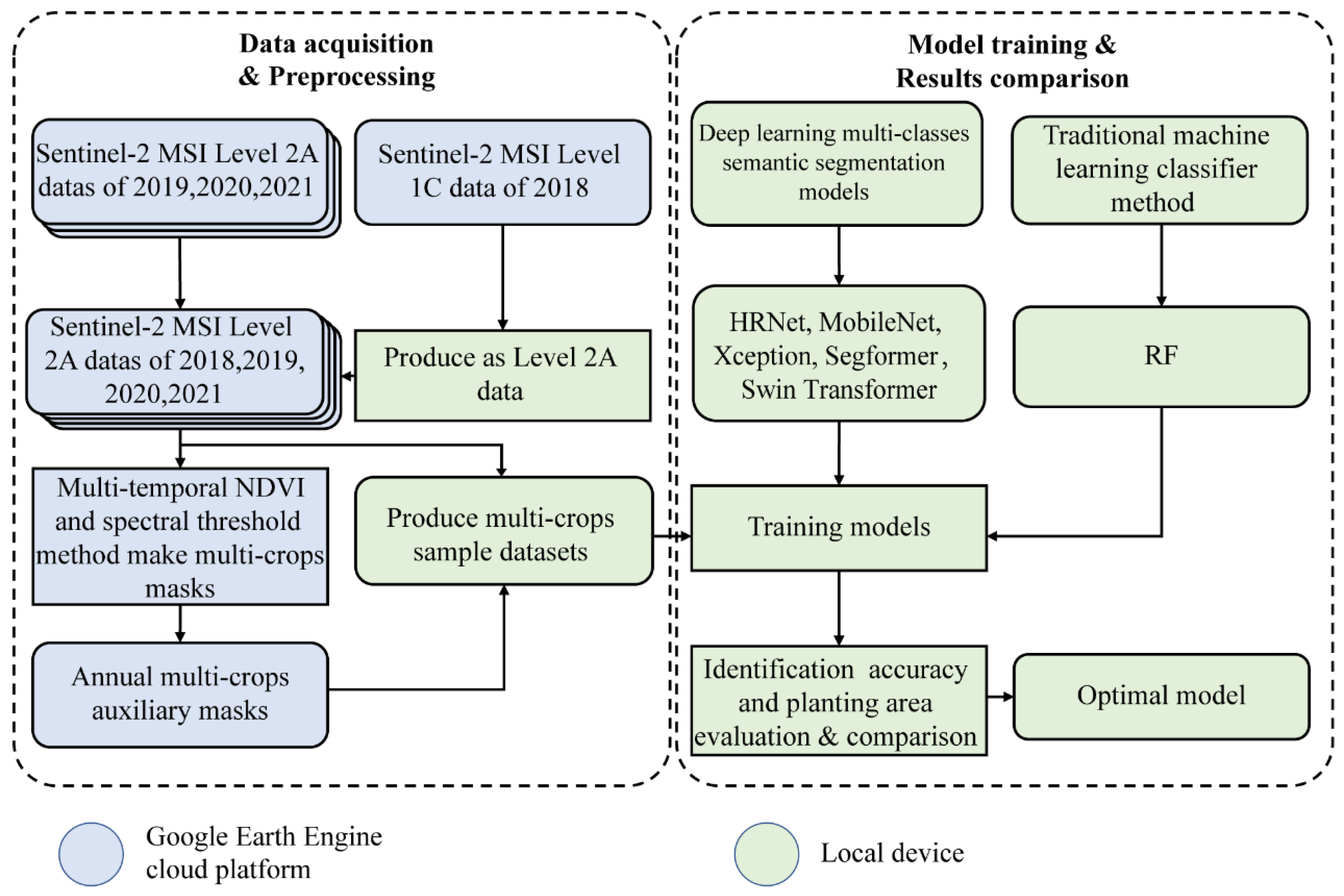
2.3.1. Data Preprocessing and Annotation

In this study, we construct paddy rice and winter wheat datasets of high-resolution Sentinel-2 MSI of farmland in Bengbu City in April from 2018 to 2021; 2019 data are used as the test set and the remaining years as the training set. Images of the dataset are labeled as paddy rice or winter wheat, using the auxiliary reference mask proposed in Section 2.2.3; paddy rice was labeled as red, winter wheat as green, and other crops and background as black. To fairly compare the performance of each network, the image patch size is kept at 256 × 256 pixels for all networks [35]. Data augmentation techniques are a data space solution to solve the limited problems of learning sample quantity and quality in supervised learning, which mainly consists of a set of techniques to increase the size and quality of the training dataset, enabling to build better DL models and maximize the use of the existing data [48]. DL models are data-intensive; to increase sample size, data augmentation techniques such as horizontal flip, vertical flip and diagonal mirroring are used to increase the sample size from 3126 to 12,648. A total of image patches from 2019 are used as the test set, while the remaining samples are used for training and validation. Figure 4 shows the samples of the paddy rice and wheat dataset and their corresponding labels in Bengbu.

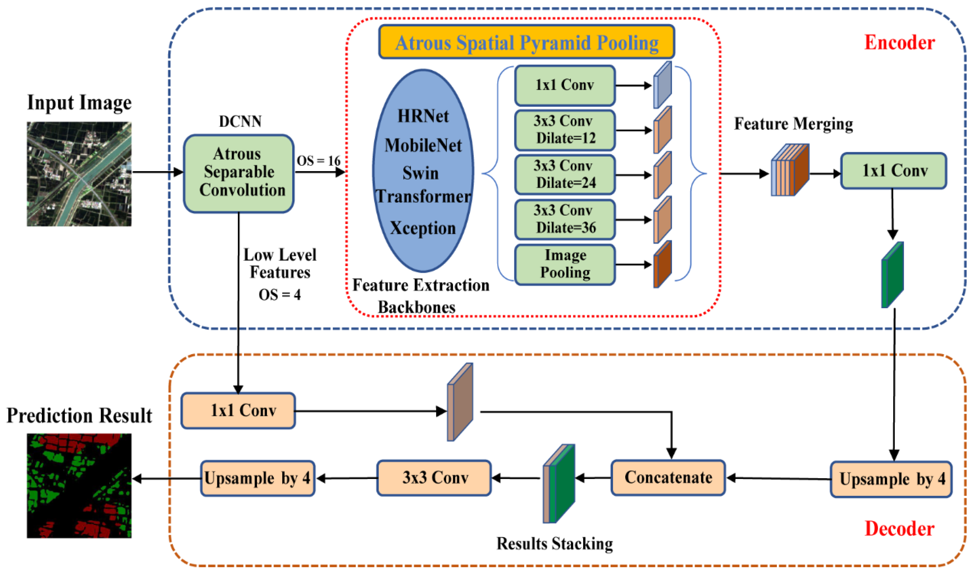
2.3.2. The Improved DeepLabv3+

DeepLabv3 is a deep convolutional neural network (DCNN) incorporating Atrous convolution [49,50,51,52], originally proposed to solve the problem of multi-scale object segmentation [53]. DeepLabv3 is designed with cascaded or parallel-running atrous convolutional modules using different atrous rates and the proposed Atrous Spatial Pyramid Pooling (ASPP) module for enhancing image-level features and capturing multi-scale semantic information [54]. Chen et al. [53] added a fast and efficient decoder module to DeepLabv3 for refining the segmentation results. They applied the Xception network to both the ASPP module and the decoder module to create DeepLabv3+.
As shown in Figure 5, the encoder section processes the input image by using the atrous convolution module to control the feature resolution and adjust the field of view of the filter for capturing multi-scale information in the DeepLabv3+ architecture; the depthwise separable convolution module reduces the computational complexity. Afterwards, the output stride (OS) parameter is set to 16 to balance the speed and accuracy of network execution. Then, three additional SS networks are embedded in the ASPP module as feature extraction backbones by us, which include a 1 × 1 convolution, a dilation convolution with different sampling rates (12, 24, 36), unlike the original DeepLabv3+, an image-level pooling for multi-scale feature extraction, and fusion and dimensionality reduction of the extracted features. The decoder part first upsampled the features generated in the encoder part by a 4-fold bilinear interpolation. The outputs are concatenated with the corresponding low-level features of the backbone network in the encoder. Finally, the stacked results pass through a 3 × 3 convolution for feature refinement and a 4-fold upsampling to produce the final prediction output.

2.3.3. HRNet, MoblieNet, Xception and Swin Transformer
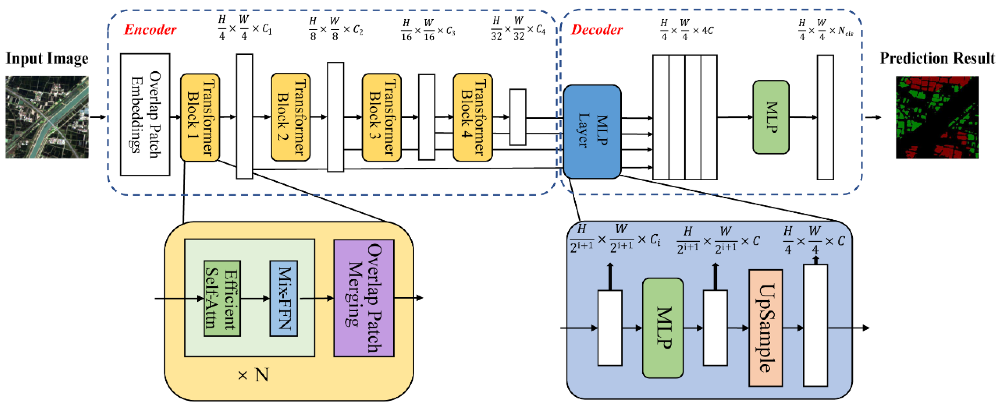
Two additional CNNs (HRNet, MobileNet) are integrated into the DeepLabv3+ architecture to extend its functionality and maximize SS performance.
HRNet consists mainly of a succession of parallel-connected convolutional subnetworks with high-to-low resolution. Each can continuously receive and fuse information from other parallel representations, thus allowing the network to retain high-resolution information throughout the structure. Sun et al. [39] made some simple modifications to improve HRNet for application to CV problems. The improved HRNet structure consists of four stages with repetitive modular multi-resolution blocks, significantly improving the network’s high-resolution solid learning and multi-level representation capabilities in SS problems. MobileNet is a class of lightweight DNNs built using deeply separable convolutions based on streamlined architecture for efficient mobile and embedded vision application models. Deeply separable convolution can significantly reduce model computational complexity compared to standard convolution. It can significantly reduce model size while allowing smaller and faster MobileNet to be built using width and resolution multipliers. Xception is also a network built using a deeply separable convolutional module, which consists of a stack called Extreme Inception; MobileNet and Xception reveal the power of deeply separable convolution from different perspectives. The Transformer [40] network structure has achieved far better results than other models in NLP because it is based entirely on the attention mechanism and does not require recursive and convolutional structures. Liu et al. [42] proposed a new visual transformer. This Swin transformer is a hierarchical visual transformer structure represented by a shifted window computation that allows flexible modeling at different scales with a linear computational complexity comparable to the image size. The shifted-windowing scheme improves model efficiency by limiting the self-attention computation to non-overlapping local windows and allowing cross-window connections [42].

2.3.4. Segformer

Segformer is a simple, efficient, and powerful SS framework in CV tasks [43,55]. The VIT [41] variant, Segformer [43], uses the Transformer structure to extract a hierarchical representation from the input image and shows better performance than previous CNNs [53,56,57,58,59] in SS. Segformer innovatively combines the Transformers structural encoder with an MLP decoder. As shown in Figure 6, the Transformer with a hierarchical structure can output multi-scale features and does not require positional coding, which allows easy adaptation to arbitrary test resolutions and avoids performance degradation due to different test and training resolutions in the encoder part. For an image with an input size of H   ×   W   ×   3 , the network divides it into 4   ×   4 sized patches. It uses them as input to the Transformer encoder for a four-stage multi-level feature extraction at 1/4, 1/8, 1/16, and 1/32 of the original image resolution. These multilevel features are passed to the All-MLP decoder for the segmentation task at the resolution of H 4   ×   W 4   ×   N cls , where N cls is the number of categories. Efficient Self-Attention, Mix-FFN and Overlapped Patch Merging are included in each hierarchical Transformer encoding block. The Efficient Self-Attention section uses the sequence reduction process to reduce the sequence length using the reduction rate (R) [60]. Mix-FFN is introduced to directly use the 3   ×   3 convolution in the feedforward network (FFN), which considers the impact of zero padding on location information leakage; this reduces network parameters and improves efficiency. The Overlapped Patch Merging process is used to generate features of the same size as the non-overlapping process by defining the patch size (K), the stride between two adjacent patches (S), and the padding size (P) [43].
Segformer also integrates a lightweight decoder consisting of only MLP layers. The decoder aggregates information from different layers and combines local and global attention for a powerful semantic representation. The All-MLP decoder consists of four main steps. First, multi-level features from the encoder are unified in the channel dimension after the MLP layer. Second, the multilevel features are upsampled to 1/4 and concatenated. After that, an MLP layer fuses the connected features. Finally, another MLP layer uses the fused features at a resolution of H 4   ×   W 4   ×   N cls for the segmentation task [43].

2.3.5. RF

The RF classifier is an integrated classifier that uses a randomly selected subset of training samples and variables to generate multiple decision trees [61]. Over the past 20 years, RF classifiers have received increasing attention due to their excellent classification results and fast processing speed [62,63,64]. In the RF’s parameterization, the number of estimators is set to 30, and the gini coefficients were used as feature evaluation metrics in the Bagging framework; the maximum number of features is set to auto, the maximum depth of the decision tree is set as default; the minimum number of samples and the minimum number of samples of leaf nodes are also set to default values.

2.4. Experimental Setup

To prevent overfitting and underfitting of the model during the network training, we set uniform training hyperparameters to put the data into the neural network for learning. For training, we set 250 total epochs, each containing 1320 iterations and the initial learning rate is set to 0.01, and the minimum learning rate is set to 0.01 times the initial learning rate with a step learning rate decay. The Adam [65] is used to optimize the weights, where the parameters β1 and β2 are set to 0.9 and 0.999, respectively. To accelerate the learning process and model convergence, we set the Nesterov momentum and weight decay to 0.9 and 0.0001, respectively. All experiments are run on a 16GB NVIDIA Tesla T4 GPU, Python 3.7 and Pytorch version 1.7.0.

2.5. Evaluation Metrics

We select the commonly used classification metrics, including overall accuracy (OA), mean Precision (mP), mean Recall (mR), mean F1 Score (mF1), Intersection over Union (IoU), mean Intersection over Union (mIoU) and training time. The OA is the number of crop pixel points correctly predicted as a proportion of the total number of crop pixel points; precision indicates the number of correctly predicted positives as a proportion of all predicted positives. Recall shows the percentage of true positives correctly predicted by the model; F1 Score is the harmonic mean of precision and recall. The IoU represents the ratio of the intersection of the network’s predictions for a crop category to the true labels, while mIoU is the average of the IoU of all crop categories. All evaluation metrics can be obtained by calculating the true positives (TP), true negatives (TN), false positives (FP) and false negatives (FN) in the confusion matrix. The equations for all indicators are shown below.
Overall   Accuracy = TP + TN TP + TN + FP + FN
Precision = TP TP + FP
Recall = TP TP + FN
F 1 = 2   ×   precision   ×   recall precision + recall
IoU n = TP n TP n + FP n + FN n
mIoU = 1 N n = 1 N IoU n
where n represents a single class, and N represents all classes.
To more intuitively analyze and compare the fitting ability of each DL network during training, focal loss [66] is introduced as the loss function. Unlike the traditional cross-entropy loss function, the focal loss function has a modulating factor, which balances the multi-classification task by increasing the weight of the less-sampled categories in the loss function and suppressing the weight of the multi-sample categories. Equation (7) is derived after adjusting the weights α and γ . Equation (9) is derived from (7) and (8).
L fl = α 1 y ^ γ l o g y ^ , i f   y = 1 1 α y ^ γ log 1 y ^ , i f   y = 0
y ^ t = y ^ , i f   y = 1 1 y ^ , o t h e r w i s e
L fl = 1 y ^ t γ log y ^ t
where α [ 0 , 1 ] is a weighting factor used to increase the weight of a few categories in the loss function and balance the loss function distribution (usually set to 0.5); γ   >   0 is similar to the adjustable weighting factor and is usually set to 2; y ^ t reflects how close the prediction result of a category is to the true value; the larger the y ^ t the more accurate the classification.

3. Results

In this section, we compare the results of each network with those of the RF method for paddy rice and winter wheat. For HRNet, MobileNet, Swin Transformer and Segformer, different size variants of these networks are tested, and the optimal number of network layers and network structure are selected to obtain the best prediction results. The results are then quantitatively analyzed.

3.1. Overall Performances Assessment

Table 1 shows the OA, mP, mR, mF1, IoU for paddy rice (RIoU), IoU for winter wheat (WIoU), IoU for other features (OIoU), mIoU and training time. The best results for all metrics are boldened. HRNet consists of two-layer types (HRNet32 and HRNet48), while MobileNet consists of two different layer types (small and large). The Swin Transformer is divided into four sizes of sub-networks (Swin_T, Swin_S, Swin_B and Swin_L). The Segformer network then selects the best feature extraction backbone. Based on the mIoU of the different sizes of networks, HRNet32, MobileNet_large, Swin_L and Segformer_B2 are selected as representative networks for the paddy rice and winter wheat mapping task.
From Table 1, the Segformer achieves the best performance regarding OA and mIoU. Segformer achieves an OA and mIoU of 91.06% and 80.70%, respectively; the mIoU is about 2.9% higher than the second-best network. HRNet32 achieves the second-best OA and mIoU at 89.84% and 77.79%, respectively. The MobileNet and Xception achieved 89.05% and 88.42% OA and 76.47% and 75.14% mIoU respectively. Network architectures strongly influenced classification performance in our experiments. Increasing the network size of the MobileNet network and Swin Transformer, significant performance improvements are achieved. Setting the same hyperparameters for all the methods could account for the poor performance of the Swin Transformer; maybe the specific hyperparameters for the Swin Transformer may improve the performance. The Swin Transformer records an mIoU of 68.17%, about 12% lower than the Segformer; the Swin Transformer only outperforms the RF. Although the RF has the highest count of misclassifications, it obtains the highest OIoU at 88.43%; the RF has significantly low RIoU and WIoU at 34.64% and 41.01%, respectively.
As this study is a multi-object classification, the P, R and F1 scores of the three categories of objects are averaged to represent the overall performance of the network. Segformer achieved the highest mP, mR and mF1 at 88.62%, 89.90% and 89.26%, respectively. HRNet32 followed closely at 87.02%, 87.77% and 87.40%, respectively. CNNs, such as MobileNet and Xception, have slightly lower mP, mR and mF1, which achieved 86.83%, 86.26% and 86.55%, 85.57%,85.74% and 85.66%, respectively. The least-performing DL method remains the Swin Transformer network, with mP, mR and mF1 values of 80.78%, 80.84% and 80.81%, respectively. RF is the worst-performing with mP, mR and mF1 values of 65.28%, 71.40% and 67.83%.
Regarding training time, HRNet32 is the slowest of all CNNs, although it achieves quite good results. Compared to the other networks, MobileNet has a considerable advantage in terms of training time consumption, requiring only 28,815 s (about 8 h) of training data, which is about 90 h less than HRNet32, and the classification results are second only to HRNet32. The training time for the Transformer architecture is generally higher than that of CNNs, with Swin Transformer taking about 170 h. Owing to Segformer’s architecture, there is a time-performance trade-off; Segformer is not the worst-performing in terms of training time and sacrificing time for better performance is acceptable. In general, there is no absolute link between training time and the final classification results of the network, but it can be used as an important evaluation indicator for method selection.
We consider the model to have converged when the loss function of our model always stays within a certain error range, and the loss value cannot be further reduced by further training. The convergence time varies greatly from model to model due to different network parameters and structures. Figure 7 depicts the training loss curves of the selected neural networks. All networks converge after the first 100 epochs. The Segformer achieves the earliest convergence and the lowest loss value within an error range; the curve remains flat and stable after the 150th epoch, with the final loss value below 0.25. HRNet32 has converged at the 50 epochs and has remained within a fairly small error range. MobileNet and Xception are very similar regarding initial loss value, error range and convergence speed. The Swin Transformer networks decrease rapidly in the first 25 epochs of training, with subsequent Loss values remaining high.
Although the supervised DL networks cannot immediately obtain the SS results of paddy rice and winter wheat, they have promising classification accuracy and generalization performance.

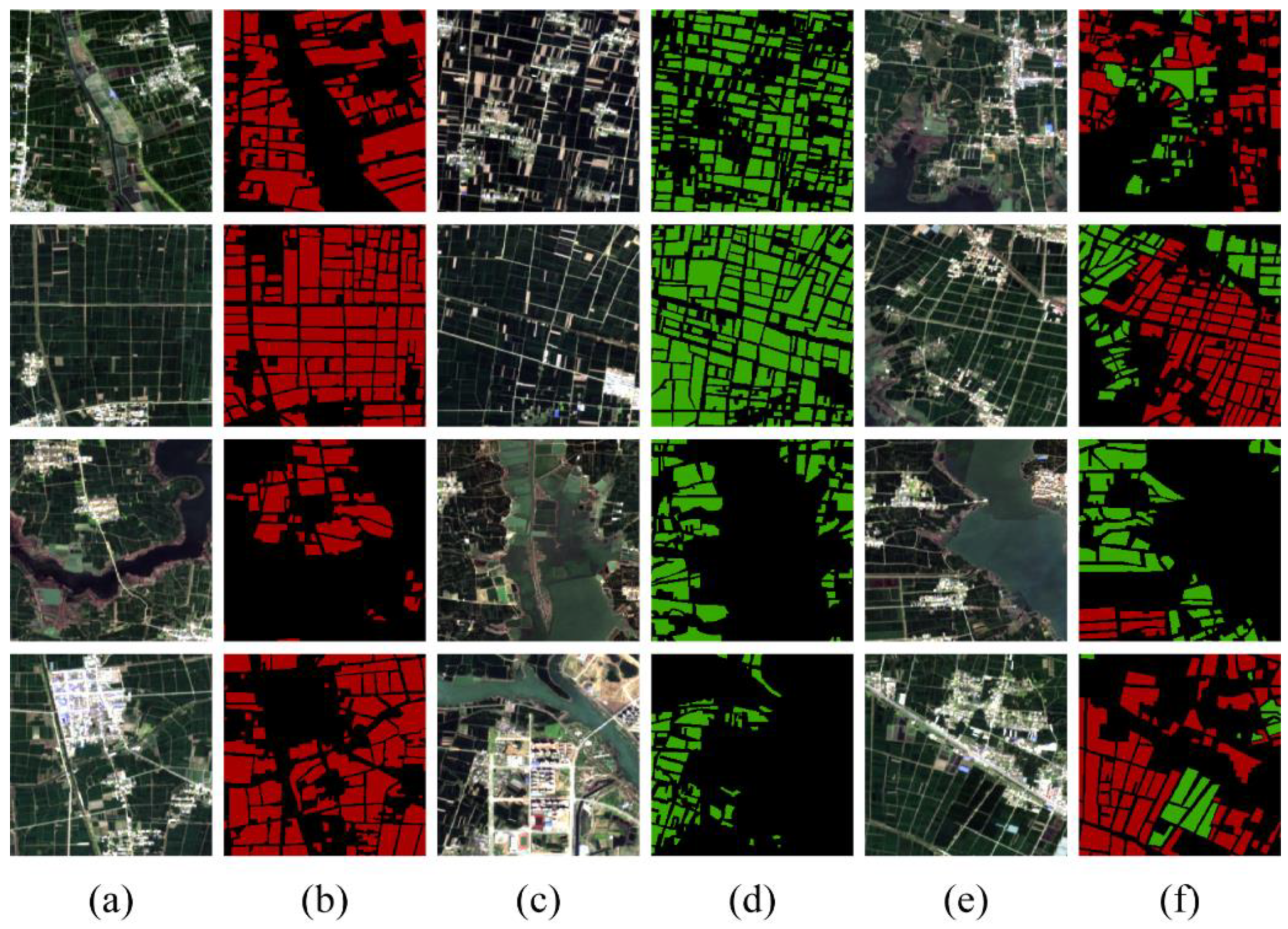
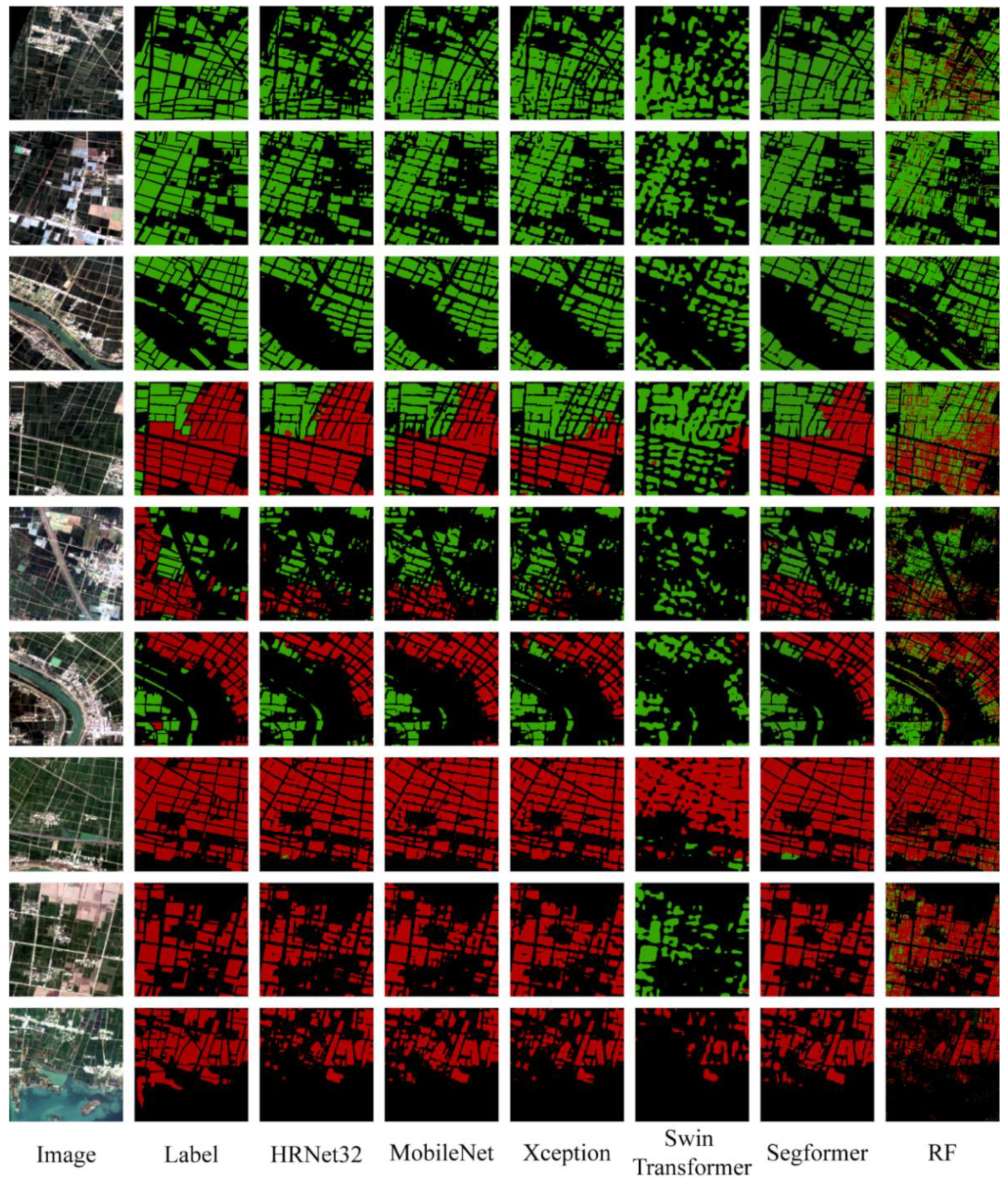
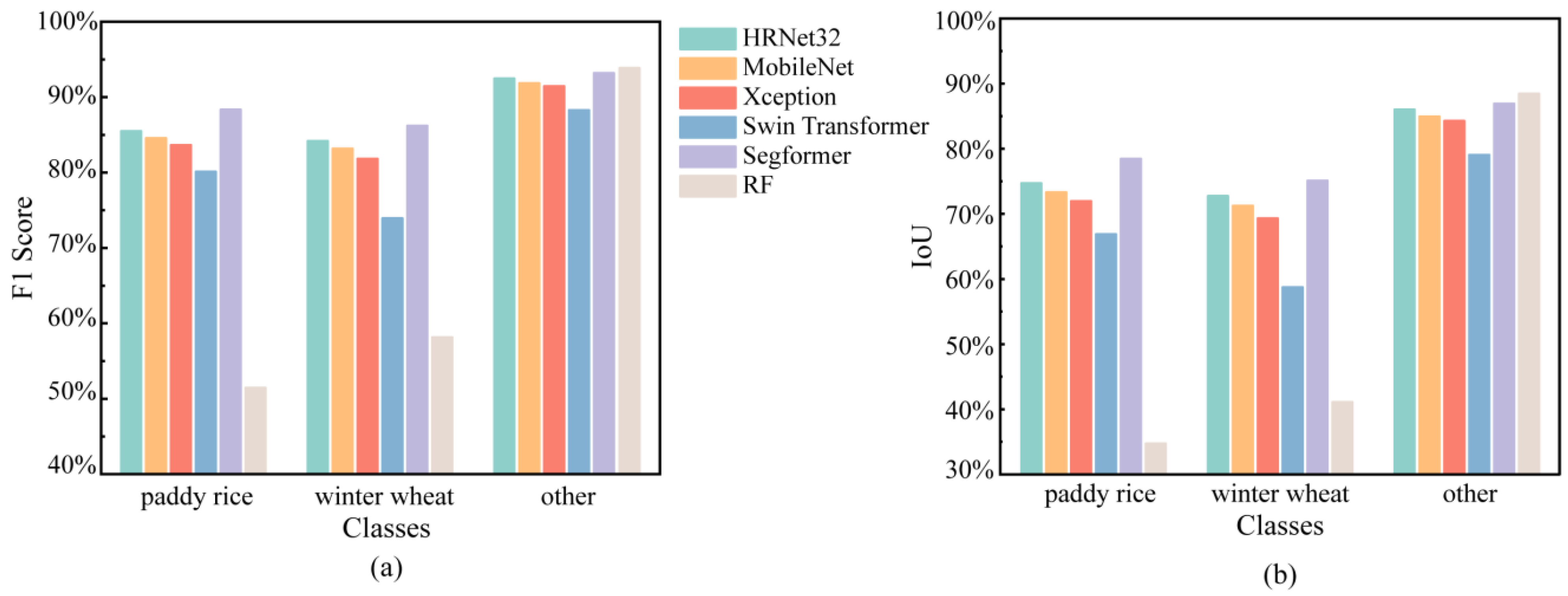
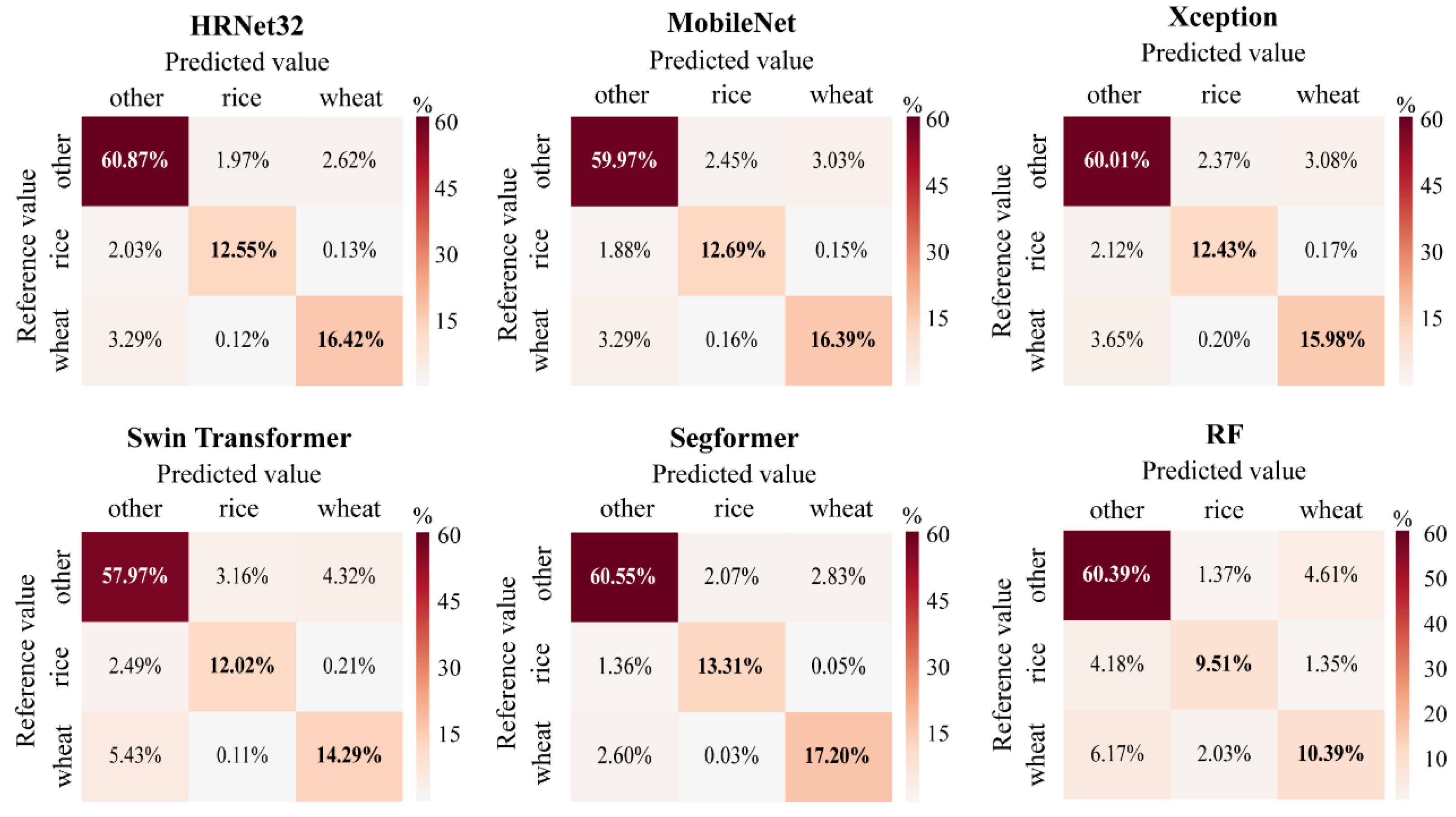
3.2. Paddy Rice and Winter Wheat Classification

To compare the classification performance of the methods in visual details, we selected several representative farmland samples from different regions in the test set. Figure 8 is the visualization results of the various methods on different farmland samples in the test set. The first and second columns show the original images and their labels, while the third the last column show the classification results of selected methods on the test set, respectively. The first three and last three rows show the classification results for winter wheat and paddy rice, respectively; the three rows in the middle show the results for the areas with mixed paddy rice and winter wheat cultivation. Different farmlands in areas with different crop cultivation types, including continuous farmland, fragmented farmland, and river-side farmland, are selected, and visualized. For the larger continuous farmland and the heavily fragmented farmland, all methods are better at removing the spectral influence of buildings, roads, bare land, and other crops on the target objects. HRNet32 showed under-identification in small and continuous winter wheat fields. However, it showed better classification results in mixed cropping areas. Except for the Swin Transformer, the other networks can identify most of the farmland contours; the edges of the farmland are well-defined, while field footpaths and country roads are clearly distinguished. Most of the networks missed small areas of farmland near the edge of waterbodies to a greater or lesser extent; the Swin Transformer network had the highest omission error, such as the complete misclassification within a broken paddy rice field; RF achieved a better performance than several DL methods in this regard. In areas with mixed cropping, the methods produced varying degrees of misclassification, mainly by misclassifying paddy rice as winter wheat; this resulted in an overestimation of the wheat area. HRNet32, MobileNet, and Segformer networks perform better in multiple-feature classification, with a significantly lower number of misclassifications than other methods; they also capture large amounts of high-resolution semantic information.
Overall, the Segformer network, with its multi-stage feature extraction Transformer encoder and lightweight decoder, achieves classification results closest to ground truth compared to the other methods. The Swin Transformer network was the worst-performing DL method with the highest misclassifications, irregular shapes of the recognized farmland, intermittent field footpath boundaries, less smooth boundaries at feature edges and significant loss of semantic information. The RF is not structured to accommodate large sample models and performs poorly on feature recognition or classification tasks with similar characteristics, resulting in high misclassifications, pepper noise within the paddy rice and winter wheat growing regions and the blurring of the boundary between the two crops. However, RF is computationally less expensive and does not rely on high-performance GPUs for advanced model training; it can obtain multi-crop classification results with some reference value in a short period.
Figure 9 shows the comparison of the F1 Score (Figure 9a) and IoU (Figure 9b) results for each category in the test set for all methods. It can be seen that for different categories, the CNNs show a similar F1 Score and IoU performance hierarchy, where HRNet32 is followed by MobileNet and Xception. The Segformer network maintained the highest F1 Score and IoU values for the two main target objects; F1 Score values are 88.35% and 86.20%, while IoU values are 79.13% and 75.74% for paddy rice and winter wheat, respectively. Swin Transformer has the worst performance among the DL methods, 13% and 17% behind Segformer for RIoU and WIoU. For the selected DL models, F1 Score and IoU for other features show Segformer as the best, followed by HRNet32, MobileNet, Xception and Swin Transformer. Although RF has many noise-like misidentifications in the field’s interior compared to other DL methods, it can significantly differentiate the spectral semantic information of other features from the main crop in the field’s exterior. Excellent segmentation results are shown on the borderline between the farm and the background. Thus, RF has the highest F1 Score and IoU values for other features. However, in the vicinity of some rivers, RF can over-identify some features belonging to other categories, such as farmland on some riverbanks, which are not paddy rice and winter wheat, resulting in an over-identification of paddy rice and winter wheat and thus affecting the F1 scores and IoU values of the two main categories.
Figure 10 shows the confusion matrix visualization for all methods on the test set. The confusion matrix demonstrates the performance of the models for each three categories. The vertical axis represents the actual values, the horizontal axis represents the predicted values, and the diagonal matrix represents the number of samples correctly predicted by the model as a percentage of the total number of test samples. In the test set, the total number of samples labelled as paddy rice and winter wheat accounted for about 32% of the entire Bengbu city, while the rest of the samples were labelled as other features. Therefore, most of the correctly identified features in the test results of the different methods belonged to other classes, and the confusion matrix blocks are shown in Figure 10.
The Segformer, for example, had a total of 14.72% of test set samples as paddy rice, of which 13.31% were correctly identified as paddy rice; 0.05% were incorrectly identified as winter wheat and 1.36% were identified as other features, having a correct recognition rate of 90.42% for paddy rice. Moreover, 17.20% of the winter wheat samples, representing 19.83% of the test set, were correctly identified; 0.03% were identified as paddy rice, and 2.60% were identified as other features, having a correct identification rate of 86.74% for winter wheat. The confusion matrix of each network shows that the Segformer has the highest number of correctly classified samples on the diagonal while it has the lowest percentage of FP and FN values among all networks. Thus, the Segformer was less influenced by other classes of semantic features during multiple-feature classification, achieving the best overall performance; HRNet32, MobileNet, Xception, and Swin Transformer followed. Except for classifying the other features, the RF generally performs worse among all methods. Except for the classification of other features, RF performed poorly among all methods, correctly identifying only 9.51% out of 15.04% paddy rice samples in the test set; 4.18% were misidentified as other features and 1.35% were misidentified as winter wheat, with an overall correct identification rate of 63.23% for paddy rice. Out of 18.59% of winter wheat samples in the test set, RF correctly identified only 10.39%, while 6.17% and 2.03% were incorrectly identified as other features and paddy rice samples, respectively; the overall correct identification rate for winter wheat was 55.89%.

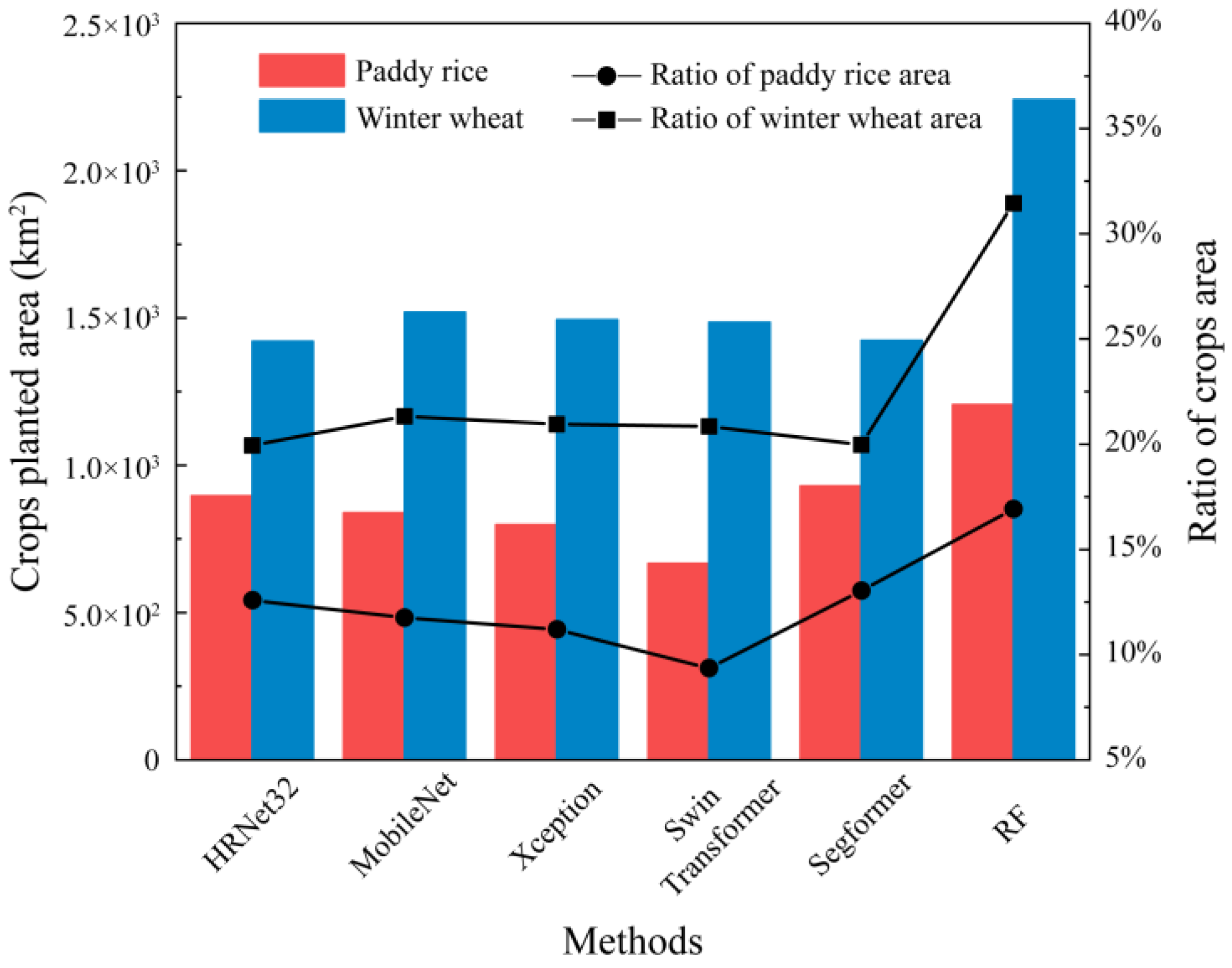
3.3. Planting Area Statistics

Figure 11 shows the statistical results of the cultivated area identified by each network for paddy rice and winter wheat on the test dataset in Bengbu in 2019 and the proportion of the area in Bengbu city. The RF identified the largest cultivated area with approximately 1200 km2 for paddy rice and 2240 km2 for winter wheat, accounting for approximately 16.92% and 31.45% of Bengbu, respectively. The high misidentification rate overestimated the area covered by paddy rice and winter wheat. The network with the smallest cultivated area identified for paddy rice was Swin Transformer at approximately 666 km2, accounting for about 9.36% of the city’s area. HRNet32 identified the smallest cultivated area for winter wheat at approximately 1421 km2, accounting for about 19.94% of the city’s area. Of the DL methods, Segformer and MobileNet identified the most paddy rice and winter wheat cultivated areas at approximately 930 km2 and 1520 km2, respectively, representing approximately 13.04% and 21.32% of the Bengbu city. As evident in Figure 9, there is a misclassification of other category as paddy rice and winter wheat in RF, which generally gives higher area statistics for both crops than the DL method. The difference between the DL methods’ estimation of winter wheat area was insignificant, with the area difference remaining at around 98.3 km2; the difference in the area for paddy rice was around 262.6 km2. However, the proportion of urban area devoted to both crops remains in the range of 30% to 33%, with most of the area of crops counted by the DL method falling within this range and RF well outside.

4. Discussion

The results show that the traditional RF approach to bi-objective crop mapping is unsatisfactory. RF cannot take advantage of the huge benefits of large data sets, and its various evaluation metrics are dwarfed by DL [67]. However, the simplicity of the RF model, the speed of classification and the fact that it does not require many samples are still great advantages. DL methods performed differently in this study, with larger amounts of data, the benefits of DL’s powerful feature extraction and non-linear relationship modelling capabilities come into play. Fairly good identification results are achieved at the expense of training time. HRNet, the classic CNN model, achieves very satisfactory mapping results but requires several days of training time. MobileNet and Xception, representatives of lightweight CNNs, achieve results second only to HRNet32 in just a few hours. Swin Transformer, a general-purpose backbone network for the Transformer architecture, may not achieve maximum performance when trained with the same amount of data as the CNN. Therefore, an appropriate SS architecture must be constructed based on its structural properties. In summary, the neural network is still performing better in mapping paddy rice and winter wheat in areas with complex cropping structures. However, there are still some problems.
Firstly, it is not enough to rely on single-temporal RS images to obtain accurate information about the actual farmland due to the complex cropping structure of real farmland, ecological fragility, and uncertainty of abandonment. There are many paddy rice and winter wheat varieties in China, and their phenological periods and spectral characteristics vary from one climatic region to another. The application of DL methods for localized classification of paddy rice and winter wheat cannot be replicated on a large scale. In the future, the combination of RS, global navigation satellite system and geographic information system technology and DL methods will enable ultra-high spatial resolution and long-time series observation satellite data, unmanned aerial vehicle data and real-time field survey data. Combined with intelligent digital image processing techniques instead of manual visual interpretation, to implement precise timing, positioning and quantitative control of important food crops or other cash crops represented by paddy rice and winter wheat. Modern intelligent agricultural production technology can maximize agricultural productivity and effectively achieve sustainable agriculture with high quality, high yield, low consumption and environmental protection [68].
Secondly, inevitable data annotation errors due to subjective factors or the influence of similar features may affect the final crop mapping results. While RS imagery is large and easy to obtain, high-quality multi-category semantic annotation data is difficult. Annotating data is often time-consuming and labour-intensive, with high labour or financial costs. In fully supervised DL, the quality of the annotated data directly affects the final results of the network. As an offshoot of unsupervised learning methods, semi-supervised learning (SSL) methods have been proposed to enable neural networks to achieve new results comparable to fully supervised networks, even when the amount of annotated data is insufficient. SSL has been applied to water body identification from RS imagery [69], but no study has applied it for multi-crop mapping from RS imagery.
Lastly, DL SS networks are developing very rapidly. With the unprecedented increase in computing power required for large models with tens of millions or even billions of parameters, there is a huge challenge in executing these models on low-end devices. In this study, the performance of the large model could not be fully exploited due to server hardware limitations, negatively impacting crop mapping results. Meanwhile, the emergence of the segment anything model (SAM) [70] has had a huge impact by improving edge detection in SS tasks [71], as well as small object identification [72], rather than focusing on overall segmentation accuracy improvement.

5. Conclusions

Multi-crop classification and mapping tasks in specific regions with more complex cropping structures are seldom explored and often have poor accuracy, with few studies focusing on paddy rice and winter wheat. This study is based on high-resolution Sentinel-2 images for simultaneous classification and bi-object mapping of two major grain crops in a typical area of eastern China. This study comprehensively evaluates several SS models’ classification and mapping performance, including CNNs, Transformer networks and RF. The main conclusions drawn are as follows:
(1)
High-resolution RS combined with DL methods are highly feasible for identifying and mapping a wide range of crops, significantly reducing the human and material costs of traditional field surveys, and compensating for the lack of quality of statistical data, which is of great importance for accurate knowledge of the crop range and food security.
(2)
The extensive experimental results show that the DL approach benefits from its powerful image-level information enhancement and multi-scale semantic feature capture; the results are far superior to traditional ML methods. In particular, the Segformer, based on the Transformers structural encoder and the lightweight MLP decoder structure, achieved an OA value of 91.06%, an mF1 value of 89.26% and a mIoU value of 80.70%, which is the best-performing network for paddy rice and winter wheat classification.
(3)
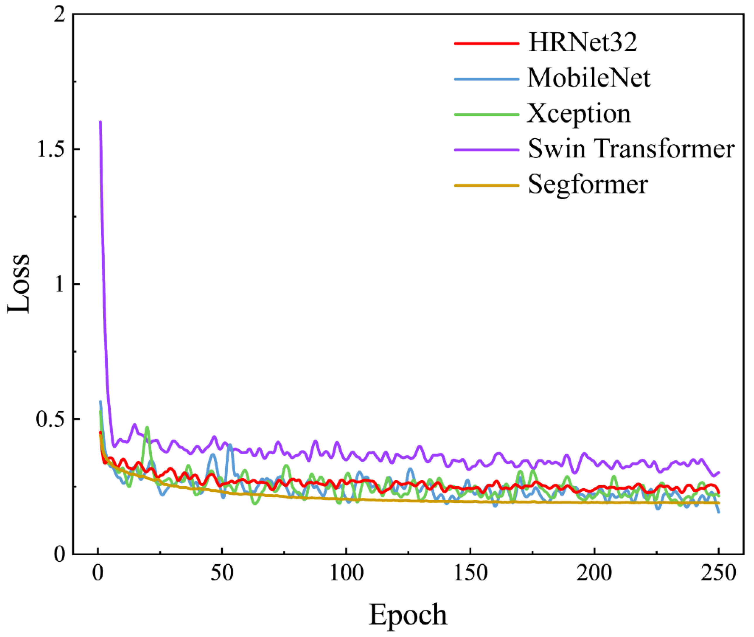
DL methods generally take longer to train than ML methods due to their complex network structure and many model parameters. The training time for the MobileNet model is only 8 h, which is the fastest convergence speed among the DL methods; it also achieves quite a good classification accuracy with high practical value. The RF method is an excellent classification method due to its short training time, low training data requirement and strong model generalization, although the final model performance is unsatisfactory.

Author Contributions

Conceptualization, W.S., G.W. and X.W.; methodology, W.S., G.W., Q.Z., X.W. and Y.H.; software, W.S., Q.Z. and Y.H.; validation, W.S.; investigation, W.S.; resources, G.W.; data curation, W.S.; writing—original draft preparation, W.S.; writing—review and editing, G.W., S.O.Y.A. and F.Z.; visualization, W.S. and Y.H.; supervision, A.F., G.W., W.D., X.W. and Y.L.; project administration, A.F. and G.W.; funding acquisition, A.F. All authors have read and agreed to the published version of the manuscript.

Funding

This research was funded by the Joint Research Project for Meteorological Capacity Improvement, grant number 22NLTSZ004; Meteorological Science and Technology Innovation Platform of China Meteorological Service Association, grant number CMSA2023MB021; the China Meteorological Administration Special Foundation for Innovation and Development, grant number of CXFZ2022J068.

Data Availability Statement

Not applicable.

Acknowledgments

This work was supported by the Joint Research Project for Meteorological Capacity Improvement (22NLTSZ004), Meteorological Science and Technology Innovation Platform of China Meteorological Service Association (CMSA2023MB021), the China Meteorological Administration Special Foundation for Innovation and Development (CXFZ2022J068).

Conflicts of Interest

The authors declare no conflict of interest.

References

  1. Zhang, X.W.; Liu, J.F.; Qin, Z.Y.; Qin, F. Winter wheat identification by integrating spectral and temporal information derived from multi-resolution remote sensing data. J. Integr. Agric. 2019, 18, 2628–2643. [Google Scholar] [CrossRef]
  2. Wang, Y.M.; Zhang, Z.; Feng, L.W.; Du, Q.Y.; Runge, T. Combining Multi-Source Data and Machine Learning Approaches to Predict Winter Wheat Yield in the Conterminous United States. Remote Sens. 2020, 12, 1232. [Google Scholar] [CrossRef] [Green Version]
  3. Ni, R.G.; Tian, J.Y.; Li, X.J.; Yin, D.M.; Li, J.W.; Gong, H.L.; Zhang, J.; Zhu, L.; Wu, D.L. An enhanced pixel-based phenological feature for accurate paddy rice mapping with Sentinel-2 imagery in Google Earth Engine. ISPRS J. Photogramm. Remote Sens. 2021, 178, 282–296. [Google Scholar] [CrossRef]
  4. Li, S.L.; Li, F.J.; Gao, M.F.; Li, Z.L.; Leng, P.; Duan, S.B.; Ren, J.Q. A New Method for Winter Wheat Mapping Based on Spectral Reconstruction Technology. Remote Sens. 2021, 13, 1810. [Google Scholar] [CrossRef]
  5. Huang, Q.; Wu, W.; Zhang, L.; Li, D. MODIS-NDVI-based crop growth monitoring in China agriculture remote sensing monitoring system. In Proceedings of the 2010 Second IITA International Conference on Geoscience and Remote Sensing, Qingdao, China, 28–31 August 2010; pp. 287–290. [Google Scholar]
  6. He, S.; Peng, P.; Chen, Y.Y.; Wang, X.M. Multi-Crop Classification Using Feature Selection-Coupled Machine Learning Classifiers Based on Spectral, Textural and Environmental Features. Remote Sens. 2022, 14, 3153. [Google Scholar] [CrossRef]
  7. Liu, J.H.; Zhu, W.Q.; Atzberger, C.; Zhao, A.Z.; Pan, Y.Z.; Huang, X. A Phenology-Based Method to Map Cropping Patterns under a Wheat-Maize Rotation Using Remotely Sensed Time-Series Data. Remote Sens. 2018, 10, 1203. [Google Scholar] [CrossRef] [Green Version]
  8. Khan, A.; Hansen, M.C.; Potapov, P.V.; Adusei, B.; Pickens, A.; Krylov, A.; Stehman, S.V. Evaluating Landsat and RapidEye Data for Winter Wheat Mapping and Area Estimation in Punjab, Pakistan. Remote Sens. 2018, 10, 489. [Google Scholar] [CrossRef] [Green Version]
  9. Jiang, M.; Xin, L.J.; Li, X.B.; Tan, M.H.; Wang, R.J. Decreasing Rice Cropping Intensity in Southern China from 1990 to 2015. Remote Sens. 2019, 11, 35. [Google Scholar] [CrossRef] [Green Version]
  10. Dong, Q.; Chen, X.H.; Chen, J.; Zhang, C.S.; Liu, L.C.; Cao, X.; Zang, Y.Z.; Zhu, X.F.; Cui, X.H. Mapping Winter Wheat in North China Using Sentinel 2A/B Data: A Method Based on Phenology-Time Weighted Dynamic Time Warping. Remote Sens. 2020, 12, 1274. [Google Scholar] [CrossRef] [Green Version]
  11. Han, J.C.; Zhang, Z.; Luo, Y.C.A.; Cao, J.; Zhang, L.L.; Cheng, F.; Zhuang, H.M.; Zhang, J.; Tao, F.L. NESEA-Rice10: High-resolution annual paddy rice maps for Northeast and Southeast Asia from 2017 to 2019. Earth Syst. Sci. Data 2021, 13, 5969–5986. [Google Scholar] [CrossRef]
  12. Chen, Y.; Yu, P.; Chen, Y.; Chen, Z. Spatiotemporal dynamics of rice–crayfish field in Mid-China and its socioeconomic benefits on rural revitalisation. Appl. Geogr. 2022, 139, 102636. [Google Scholar] [CrossRef]
  13. Frolking, S.; Qiu, J.; Boles, S.; Xiao, X.; Liu, J.; Zhuang, Y.; Li, C.; Qin, X. Combining remote sensing and ground census data to develop new maps of the distribution of rice agriculture in China. Glob. Biogeochem. Cycles 2002, 16, 38-1–38-10. [Google Scholar] [CrossRef] [Green Version]
  14. Cheng, H.; Ren, W.; Ding, L.; Liu, Z.; Fang, C. Responses of a rice–wheat rotation agroecosystem to experimental warming. Ecol. Res. 2013, 28, 959–967. [Google Scholar] [CrossRef]
  15. Khatami, R.; Mountrakis, G.; Stehman, S.V. A meta-analysis of remote sensing research on supervised pixel-based land-cover image classification processes: General guidelines for practitioners and future research. Remote Sens. Environ. 2016, 177, 89–100. [Google Scholar] [CrossRef] [Green Version]
  16. King, L.; Adusei, B.; Stehman, S.V.; Potapov, P.V.; Song, X.-P.; Krylov, A.; Di Bella, C.; Loveland, T.R.; Johnson, D.M.; Hansen, M.C. A multi-resolution approach to national-scale cultivated area estimation of soybean. Remote Sens. Environ. 2017, 195, 13–29. [Google Scholar] [CrossRef]
  17. Löw, F.; Michel, U.; Dech, S.; Conrad, C. Impact of feature selection on the accuracy and spatial uncertainty of per-field crop classification using support vector machines. ISPRS J. Photogramm. Remote Sens. 2013, 85, 102–119. [Google Scholar] [CrossRef]
  18. Massey, R.; Sankey, T.T.; Congalton, R.G.; Yadav, K.; Thenkabail, P.S.; Ozdogan, M.; Meador, A.J.S. MODIS phenology-derived, multi-year distribution of conterminous US crop types. Remote Sens. Environ. 2017, 198, 490–503. [Google Scholar] [CrossRef]
  19. Shi, D.; Yang, X. An assessment of algorithmic parameters affecting image classification accuracy by random forests. Photogramm. Eng. Remote Sens. 2016, 82, 407–417. [Google Scholar] [CrossRef]
  20. Xu, J.; Zhu, Y.; Zhong, R.; Lin, Z.; Xu, J.; Jiang, H.; Huang, J.; Li, H.; Lin, T. DeepCropMapping: A multi-temporal deep learning approach with improved spatial generalizability for dynamic corn and soybean mapping. Remote Sens. Environ. 2020, 247, 111946. [Google Scholar] [CrossRef]
  21. Azzari, G.; Lobell, D.B. Landsat-based classification in the cloud: An opportunity for a paradigm shift in land cover monitoring. Remote Sens. Environ. 2017, 202, 64–74. [Google Scholar] [CrossRef]
  22. Saini, R.; Ghosh, S.K. Crop classification in a heterogeneous agricultural environment using ensemble classifiers and single-date Sentinel-2A imagery. Geocarto Int. 2021, 36, 2141–2159. [Google Scholar] [CrossRef]
  23. Breiman, L. Random forests. Mach. Learn. 2001, 45, 5–32. [Google Scholar] [CrossRef] [Green Version]
  24. Prins, A.J.; Van Niekerk, A. Crop type mapping using LiDAR, Sentinel-2 and aerial imagery with machine learning algorithms. Geo-Spat. Inf. Sci. 2021, 24, 215–227. [Google Scholar] [CrossRef]
  25. Maggiori, E.; Tarabalka, Y.; Charpiat, G.; Alliez, P. Convolutional Neural Networks for Large-Scale Remote-Sensing Image Classification. IEEE T Geosci. Remote 2017, 55, 645–657. [Google Scholar] [CrossRef] [Green Version]
  26. Zhang, L.; Liu, Z.; Ren, T.W.; Liu, D.Y.; Ma, Z.; Tong, L.; Zhang, C.; Zhou, T.Y.; Zhang, X.D.; Li, S.M. Identification of Seed Maize Fields with High Spatial Resolution and Multiple Spectral Remote Sensing Using Random Forest Classifier. Remote Sens. 2020, 12, 362. [Google Scholar] [CrossRef] [Green Version]
  27. Kussul, N.; Lavreniuk, M.; Skakun, S.; Shelestov, A. Deep Learning Classification of Land Cover and Crop Types Using Remote Sensing Data. IEEE Geosci. Remote Sens. Lett. 2017, 14, 778–782. [Google Scholar] [CrossRef]
  28. Marcos, D.; Volpi, M.; Kellenberger, B.; Tuia, D. Land cover mapping at very high resolution with rotation equivariant CNNs: Towards small yet accurate models. ISPRS J. Photogramm. Remote Sens. 2018, 145, 96–107. [Google Scholar] [CrossRef] [Green Version]
  29. Krizhevsky, A.; Sutskever, I.; Hinton, G.E. Imagenet classification with deep convolutional neural networks. Commun. ACM 2017, 60, 84–90. [Google Scholar] [CrossRef] [Green Version]
  30. Simonyan, K.; Zisserman, A. Very deep convolutional networks for large-scale image recognition. arXiv 2014, arXiv:1409.1556. [Google Scholar]
  31. Howard, A.G.; Zhu, M.; Chen, B.; Kalenichenko, D.; Wang, W.; Weyand, T.; Andreetto, M.; Adam, H. Mobilenets: Efficient convolutional neural networks for mobile vision applications. arXiv 2017, arXiv:1704.04861. [Google Scholar] [CrossRef]
  32. Szegedy, C.; Liu, W.; Jia, Y.; Sermanet, P.; Reed, S.; Anguelov, D.; Erhan, D.; Vanhoucke, V.; Rabinovich, A. Going deeper with convolutions. In Proceedings of the IEEE Conference on Computer Vision and Pattern Recognition, Boston, MA, USA, 7–12 June 2015; pp. 1–9. [Google Scholar]
  33. Chollet, F. Xception: Deep learning with depthwise separable convolutions. In Proceedings of the IEEE Conference on Computer Vision and Pattern Recognition, Honolulu, HI, USA, 21–26 July 2017; pp. 1251–1258. [Google Scholar]
  34. Ronneberger, O.; Fischer, P.; Brox, T. U-net: Convolutional networks for biomedical image segmentation. In Proceedings of the Medical Image Computing and Computer-Assisted Intervention—MICCAI 2015: 18th International Conference, Munich, Germany, 5–9 October 2015; pp. 234–241. [Google Scholar]
  35. Dong, Z.; Wang, G.J.; Amankwah, S.O.Y.; Wei, X.K.; Hu, Y.F.; Feng, A.Q. Monitoring the summer flooding in the Poyang Lake area of China in 2020 based on Sentinel-1 data and multiple convolutional neural networks. Int. J. Appl. Earth Obs. Geoinf. 2021, 102, 102400. [Google Scholar] [CrossRef]
  36. Fourure, D.; Emonet, R.; Fromont, E.; Muselet, D.; Tremeau, A.; Wolf, C. Residual conv-deconv grid network for semantic segmentation. arXiv 2017, arXiv:1707.07958. [Google Scholar]
  37. Huang, G.; Liu, Z.; Van Der Maaten, L.; Weinberger, K.Q. Densely connected convolutional networks. In Proceedings of the IEEE Conference on Computer Vision and Pattern Recognition, Honolulu, HI, USA, 21–26 July 2017; pp. 4700–4708. [Google Scholar]
  38. Wang, J.; Sun, K.; Cheng, T.; Jiang, B.; Deng, C.; Zhao, Y.; Liu, D.; Mu, Y.; Tan, M.; Wang, X. Deep high-resolution representation learning for visual recognition. IEEE Trans. Pattern Anal. Mach. Intell. 2020, 43, 3349–3364. [Google Scholar] [CrossRef] [PubMed] [Green Version]
  39. Sun, K.; Zhao, Y.; Jiang, B.; Cheng, T.; Xiao, B.; Liu, D.; Mu, Y.; Wang, X.; Liu, W.; Wang, J. High-resolution representations for labeling pixels and regions. arXiv 2019, arXiv:1904.04514. [Google Scholar]
  40. Vaswani, A.; Shazeer, N.; Parmar, N.; Uszkoreit, J.; Jones, L.; Gomez, A.N.; Kaiser, Ł.; Polosukhin, I. Attention is all you need. In Proceedings of the Advances in Neural Information Processing Systems, Long Beach, CA, USA, 4–9 December 2017; Volume 30. [Google Scholar] [CrossRef]
  41. Dosovitskiy, A.; Beyer, L.; Kolesnikov, A.; Weissenborn, D.; Zhai, X.; Unterthiner, T.; Dehghani, M.; Minderer, M.; Heigold, G.; Gelly, S. An image is worth 16x16 words: Transformers for image recognition at scale. arXiv 2020, arXiv:2010.11929. [Google Scholar]
  42. Liu, Z.; Lin, Y.; Cao, Y.; Hu, H.; Wei, Y.; Zhang, Z.; Lin, S.; Guo, B. Swin transformer: Hierarchical vision transformer using shifted windows. In Proceedings of the IEEE/CVF International Conference on Computer Vision, Montreal, BC, Canada, 11–17 October 2021; pp. 10012–10022. [Google Scholar]
  43. Xie, E.; Wang, W.; Yu, Z.; Anandkumar, A.; Alvarez, J.M.; Luo, P. SegFormer: Simple and efficient design for semantic segmentation with transformers. Adv. Neural Inf. Process. Syst. 2021, 34, 12077–12090. [Google Scholar] [CrossRef]
  44. Wang, X.; Zhang, J.H.; Xun, L.; Wang, J.W.; Wu, Z.J.; Henchiri, M.; Zhang, S.C.; Zhang, S.; Bai, Y.; Yang, S.S.; et al. Evaluating the Effectiveness of Machine Learning and Deep Learning Models Combined Time-Series Satellite Data for Multiple Crop Types Classification over a Large-Scale Region. Remote Sens. 2022, 14, 2341. [Google Scholar] [CrossRef]
  45. Sun, K.; Xiao, B.; Liu, D.; Wang, J. Deep high-resolution representation learning for human pose estimation. In Proceedings of the IEEE/CVF Conference on Computer Vision and Pattern Recognition, Long Beach, CA, USA, 15–20 June 2019; pp. 5693–5703. [Google Scholar]
  46. Zuo, Q.; Chen, Y.; Tao, J. Climate change and its impact on water resources in the Huai River Basin. Bull. Chin. Acad. Sci. 2012, 26, 32–39. [Google Scholar]
  47. Xu, D.; Fu, M.C. Detection and Modeling of Vegetation Phenology Spatiotemporal Characteristics in the Middle Part of the Huai River Region in China. Sustainability 2015, 7, 2841–2857. [Google Scholar] [CrossRef] [Green Version]
  48. Shorten, C.; Khoshgoftaar, T.M. A survey on Image Data Augmentation for Deep Learning. J. Big Data 2019, 6, 60. [Google Scholar] [CrossRef] [Green Version]
  49. Sermanet, P.; Eigen, D.; Zhang, X.; Mathieu, M.; Fergus, R.; LeCun, Y. Overfeat: Integrated recognition, localization and detection using convolutional networks. arXiv 2013, arXiv:1312.6229. [Google Scholar]
  50. Papandreou, G.; Kokkinos, I.; Savalle, P.-A. Modeling local and global deformations in deep learning: Epitomic convolution, multiple instance learning, and sliding window detection. In Proceedings of the IEEE Conference on Computer Vision and Pattern Recognition, Boston, MA, USA, 7–12 June 2015; pp. 390–399. [Google Scholar]
  51. Holschneider, M.; Kronland-Martinet, R.; Morlet, J.; Tchamitchian, P. A real-time algorithm for signal analysis with the help of the wavelet transform. In Proceedings of the Wavelets: Time-Frequency Methods and Phase Space Proceedings of the International Conference; Marseille, France, 14–18 December 1987, 1990; pp. 286–297. [Google Scholar]
  52. Giusti, A.; Cireşan, D.C.; Masci, J.; Gambardella, L.M.; Schmidhuber, J. Fast image scanning with deep max-pooling convolutional neural networks. In Proceedings of the 2013 IEEE International Conference on Image Processing, Melbourne, Australia, 15–18 September 2013; pp. 4034–4038. [Google Scholar]
  53. Chen, L.-C.; Zhu, Y.; Papandreou, G.; Schroff, F.; Adam, H. Encoder-decoder with atrous separable convolution for semantic image segmentation. In Proceedings of the European Conference on Computer Vision (ECCV), Munich, Germany, 8–14 September 2018; pp. 801–818. [Google Scholar]
  54. Chen, L.-C.; Papandreou, G.; Schroff, F.; Adam, H. Rethinking atrous convolution for semantic image segmentation. arXiv 2017, arXiv:1706.05587. [Google Scholar]
  55. Bai, H.; Mao, H.; Nair, D. Dynamically pruning segformer for efficient semantic segmentation. In Proceedings of the ICASSP 2022—2022 IEEE International Conference on Acoustics, Speech and Signal Processing (ICASSP), Singapore, 22–27 May 2022; pp. 3298–3302. [Google Scholar]
  56. Chen, L.-C.; Papandreou, G.; Kokkinos, I.; Murphy, K.; Yuille, A.L. Deeplab: Semantic image segmentation with deep convolutional nets, atrous convolution, and fully connected crfs. IEEE Trans. Pattern Anal. Mach. Intell. 2017, 40, 834–848. [Google Scholar] [CrossRef] [Green Version]
  57. Long, J.; Shelhamer, E.; Darrell, T. Fully convolutional networks for semantic segmentation. In Proceedings of the IEEE Conference on Computer Vision and Pattern Recognition, Boston, MA, USA, 7–12 June 2015; pp. 3431–3440. [Google Scholar]
  58. Zhao, H.; Qi, X.; Shen, X.; Shi, J.; Jia, J. Icnet for real-time semantic segmentation on high-resolution images. In Proceedings of the European Conference on Computer Vision (ECCV), Munich, Germany, 8–14 September 2018; pp. 405–420. [Google Scholar]
  59. Zhao, H.; Shi, J.; Qi, X.; Wang, X.; Jia, J. Pyramid scene parsing network. In Proceedings of the IEEE Conference on Computer Vision and Pattern Recognition, Honolulu, HI, USA, 21–26 July 2017; pp. 2881–2890. [Google Scholar]
  60. Wang, W.; Xie, E.; Li, X.; Fan, D.-P.; Song, K.; Liang, D.; Lu, T.; Luo, P.; Shao, L. Pyramid vision transformer: A versatile backbone for dense prediction without convolutions. In Proceedings of the IEEE/CVF International Conference on Computer Vision, Montreal, BC, Canada, 11–17 October 2021; pp. 568–578. [Google Scholar]
  61. Belgiu, M.; Dragut, L. Random forest in remote sensing: A review of applications and future directions. ISPRS J. Photogramm. Remote Sens. 2016, 114, 24–31. [Google Scholar] [CrossRef]
  62. Rodriguez-Galiano, V.F.; Ghimire, B.; Rogan, J.; Chica-Olmo, M.; Rigol-Sanchez, J.P. An assessment of the effectiveness of a random forest classifier for land-cover classification. ISPRS J. Photogramm. Remote Sens. 2012, 67, 93–104. [Google Scholar] [CrossRef]
  63. Pal, M. Random forest classifier for remote sensing classification. Int. J. Remote Sens. 2005, 26, 217–222. [Google Scholar] [CrossRef]
  64. Du, P.J.; Samat, A.; Waske, B.; Liu, S.C.; Li, Z.H. Random Forest and Rotation Forest for fully polarized SAR image classification using polarimetric and spatial features. ISPRS J. Photogramm. Remote Sens. 2015, 105, 38–53. [Google Scholar] [CrossRef]
  65. Kingma, D.P.; Ba, J. Adam: A method for stochastic optimization. arXiv 2014, arXiv:1412.6980. [Google Scholar] [CrossRef]
  66. Lin, T.-Y.; Goyal, P.; Girshick, R.; He, K.; Dollár, P. Focal loss for dense object detection. In Proceedings of the IEEE International Conference on Computer Vision, Venice, Italy, 22–29 October 2017; pp. 2980–2988. [Google Scholar]
  67. Wang, G.; Wu, M.; Wei, X.; Song, H. Water identification from high-resolution remote sensing images based on multidimensional densely connected convolutional neural networks. Remote Sens. 2020, 12, 795. [Google Scholar] [CrossRef] [Green Version]
  68. Elert, E. Rice by the numbers: A good grain. Nature 2014, 514, S50. [Google Scholar] [CrossRef] [PubMed] [Green Version]
  69. Dang, B.; Li, Y.S. MSResNet: Multiscale Residual Network via Self-Supervised Learning for Water-Body Detection in Remote Sensing Imagery. Remote Sens. 2021, 13, 3122. [Google Scholar] [CrossRef]
  70. Kirillov, A.; Mintun, E.; Ravi, N.; Mao, H.; Rolland, C.; Gustafson, L.; Xiao, T.; Whitehead, S.; Berg, A.C.; Lo, W.-Y. Segment anything. arXiv 2023, arXiv:2304.02643. [Google Scholar]
  71. Takikawa, T.; Acuna, D.; Jampani, V.; Fidler, S. Gated-scnn: Gated shape cnns for semantic segmentation. In Proceedings of the IEEE/CVF International Conference on Computer Vision, Seoul, Republic of Korea, 27 October–2 November 2019; pp. 5229–5238. [Google Scholar]
  72. Li, X.; Zhao, H.; Han, L.; Tong, Y.; Tan, S.; Yang, K. Gated fully fusion for semantic segmentation. In Proceedings of the AAAI Conference on Artificial Intelligence, New York, NY, USA, 7–12 February 2020; pp. 11418–11425. [Google Scholar]
Figure 1. The location of Anhui Province in China and Bengbu City in Anhui Province (a); Overview of the distribution of rivers and lakes in and around Bengbu (b). The background is a topographical map of Bengbu City.
Remotesensing 15 03417 g001
Figure 2. Phenology calendar of major crops in Bengbu.
Remotesensing 15 03417 g002
Figure 3. Schematic diagram of the workflow of this study. Including local processing and Google Earth Engine (GEE) cloud platform processing.
Remotesensing 15 03417 g003
Figure 4. Sentinel-2 images of paddy rice and winter wheat in Bengbu and their corresponding labels, including crushed farmlands, large-scale continuous farmlands, riverside farmlands and farmlands next to buildings. Where the red part represents paddy rice and the green represents winter wheat. Columns (a,c,e) are the original images, and columns (b,d,f) are the corresponding labels.
Remotesensing 15 03417 g004
Figure 5. The improved DeepLabv3+ architecture with an encoder-decoder structure and atrous spatial pyramid pooling (ASPP). The green part is the feature extraction part of the encoder, the blue part is the feature extraction backbone network, and the light brown part is the decoder.
Remotesensing 15 03417 g005
Figure 6. The overall architecture of Segformer. The yellow part represents the layered Transformer encoder and the blue represents the lightweight multilayer perceptron (MLP) decoder.
Remotesensing 15 03417 g006
Figure 7. Training loss curve of deep learning networks.
Remotesensing 15 03417 g007
Figure 8. Comparison of multi-crops classification results by all networks in Bengbu on the test set. The red part represents rice while the green part represents winter wheat. The first three rows represent winter wheat cultivation, the next three rows are paddy rice mixed with winter wheat, and the last three rows show the results for paddy rice cultivation.
Remotesensing 15 03417 g008
Figure 9. Comparison of the F1 scores (a) and Intersection over Union (IoU) indicators (b) for each class with all models on the test set.
Remotesensing 15 03417 g009
Figure 10. Confusion matrix of all models on the test set. The values in the confusion matrix represent the number of samples in that matrix as a percentage of the total number. The boldened values on the diagonal line represent the number of samples correctly classified.
Remotesensing 15 03417 g010
Figure 11. Differences in the area and proportion of paddy rice and winter wheat cultivation in Bengbu identified by all networks on the test set.
Remotesensing 15 03417 g011
Table 1. The comparison of model performance based on selected metrics. The optimal value for each metric is shown in bold.
OAmPmRmF1RIoUWIoUOIoUmIoUTime
HRNet3289.84%87.02%87.77%87.40%74.67%72.71%86.00%77.79%351,201 s
MobileNet89.05%86.83%86.26%86.55%73.27%71.21%84.92%76.47%28,815 s
Xception88.42%85.57%85.74%85.66%71.91%69.25%84.25%75.14%119,003 s
STSF84.29%80.78%80.84%80.81%66.83%58.66%79.02%68.17%611,899 s
Segformer91.06%88.62%89.90%89.26%79.13%75.74%87.24%80.70%159,933 s
RF87.65%65.28%71.40%67.83%34.64%41.01%88.43%54.69%____
Disclaimer/Publisher’s Note: The statements, opinions and data contained in all publications are solely those of the individual author(s) and contributor(s) and not of MDPI and/or the editor(s). MDPI and/or the editor(s) disclaim responsibility for any injury to people or property resulting from any ideas, methods, instructions or products referred to in the content.

