Multi-Branch Deep Learning Framework for Land Scene Classification in Satellite Imagery

Abstract

Land scene classification in satellite imagery has a wide range of applications in remote surveillance, environment monitoring, remote scene analysis, Earth observations and urban planning. Due to immense advantages of the land scene classification task, several methods have been proposed during recent years to automatically classify land scenes in remote sensing images. Most of the work focuses on designing and developing deep networks to identify land scenes from high-resolution satellite images. However, these methods face challenges in identifying different land scenes. Complex texture, cluttered background, extremely small size of objects and large variations in object scale are the common challenges that restrict the models to achieve high performance. To tackle these challenges, we propose a multi-branch deep learning framework that efficiently combines global contextual features with multi-scale features to identify complex land scenes. Generally, the framework consists of two branches. The first branch extracts global contextual information from different regions of the input image, and the second branch exploits a fully convolutional network (FCN) to extract multi-scale local features. The performance of the proposed framework is evaluated on three benchmark datasets, UC-Merced, SIRI-WHU, and EuroSAT. From the experiments, we demonstrate that the framework achieves superior performance compared to other similar models.

1. Introduction

With the advancements in remote sensing technologies, considerable amount of satellite data can be easily acquired [1]. The availability of high-resolution satellite images opens new opportunities and challenges for researchers and scientists from the remote sensing community. During recent years, researchers and scientists have utilized remote sensing data to explore various semantic tasks such as road segmentation [2], land cover semantic segmentation [3] and classification [4], building extraction [5], farmland segmentation [6], and multiple geo-spatial objects detection [7]. Among these semantic tasks, land cover classification has achieved tremendous attention from the research community due to its wide applications in various fields. The task of land cover classification is to identify the scene, given the remote sensing image. Such information can be utilized in urban planning [8,9], disaster assessment [10], landslide hazards [11], monitoring of ecosystems [12], depletion of ground water [13], crop fields [14], etc.

Several methods and techniques have been proposed in the literature to classify land cover patterns. Generally, we categorize these methods into two major groups: (1) unsupervised and (2) supervised methods. The unsupervised methods adopt various clustering techniques, for example, fuzzy c-means [15], K-means [16], etc., to identify the patterns in satellite images. We further categorize supervised techniques into two groups: (1) handcrafted features and (2) deep hierarchical features. The handcrafted-features-based techniques extract discriminating features and employ statistical machine learning models, for example, SVM [17], random forest [18], and decision trees [19], to identify different land patterns in satellite images. Deep learning models, on the other hand, automatically learn deep hierarchical features from the raw images [20].

Convolutional neural networks (CNNs) are recognized as the most powerful and mainstream models for various classification [21], object detection [7] and segmentation tasks [3]. Deep learning models automatically capture rich contextual information and learn hierarchical features from various layers of CNN models.

Despite immense success of deep learning models in natural images (captured on the ground level), the performance of deep learning models in land cover classification tasks in remote sensing images still suffers from the following limitations: (1) The size of objects in satellite images is very small, and they usually cover a small portion of the whole image [22], as shown in Figure 1 (left). This problem will lead the network to learn a large amount of useless features, and the network may not be able to learn important discriminating features. (2) There is a large variation in object scales in remote sensing images [7]. For example, as shown in Figure 1, the size of an airplane in an image on the left is relatively small versus the size of the airplane in the image on the right. Due to this problem, most single-scale or fixed-scale models cannot extract multi-scale features that are crucial for the classification task in satellite imagery.

In order to address the above-mentioned problems, we propose a multi-branch framework for the land cover classification task in high-resolution satellite images. Generally, the proposed framework consists of two branches. The first branch is the global contextual module that ingrates a convolutional neural network (DenseNet) with the pyramid pooling module to extract contextual information from various regions of the input image. The second branch is the local feature extraction module that exploits a fully convolutional neural network (FCN) and extracts multi-scale local features.

The concept of multi-branch or combining two deep learning models has gained significant attraction from the research community and has been successfully employed in numerous domains. By combining two deep learning models, researchers and practitioners can leverage the strengths and diverse representations of each individual model. This allows for a more comprehensive analysis of complex data and for the extraction of meaningful insights. A multi-branch deep learning framework is proposed in [23] that combines a convolutional neural network with a recursive neural network for blood cell image classification. Similarly, the method in [24] combines a graph neural network and CNN for hyperspectral image classification. A multi-column deep learning network is proposed in [25] for digit image classification. In [26], the authors proposed a framework for image classification that combines both deep learning features and handcrafted features. A two-stage deep model is proposed in [27] for painting classification. The success of multi-branch networks in classifying natural images has led researchers to develop dedicated multi-branch models for the purpose of scene classification in remote sensing images. For example, the authors proposed a two-stream architecture, namely, structure key area localization (SKAL) for image classification in high-resolution satellite images. Similarly, a dual-branch structure model, namely, GLDBS, is proposed in [28] for scene classification in remote sensing images. Although the proposed multi-branch framework follows a similar pipeline to that of the SKAL and GLDBS models, it distinguishes itself in the following ways.

Comparisons and Differences: The proposed framework is apparently similar to the SKAL-based two-stream architecture [22] and global–local dual-branch structure (GLDBS) [28]. However, the proposed framework differs in the following ways:

• The global streams of both the SKAL and GLDBS frameworks use feature maps of the last convolutional layer for classification. This strategy reduces the discriminating capability of the framework by ignoring the important information hidden in various layers of the network. Moreover, these frameworks have limitations in effectively aggregating global contextual information, which often results in misclassification of visually similar but distinct objects. In contrast, the proposed framework integrates the pyramid pooling module to incorporate more contextual information from various regions of the input feature maps.
• The local streams of both the SKAL and GLDBS frameworks utilize a convolutional neural network (CNN) to identify the coarse locations and scales of objects in the scene. Due to this strategy, the frameworks are unable to obtain fine-grained features from the local regions, and they lead to background noise. In contrast, the local branch of the proposed framework employs a two-stage model by exploiting a fully convolutional network (FCN). The model first generates multi-scale object proposals (corresponding to the local region of the image) and then extracts discriminating features from important local areas (object proposals) of the input image.

Considering the limitations of previous methods, the contributions of the proposed work are listed as follows:

1.

A multi-branch deep learning framework is proposed for land scene classification in satellite images.

2.

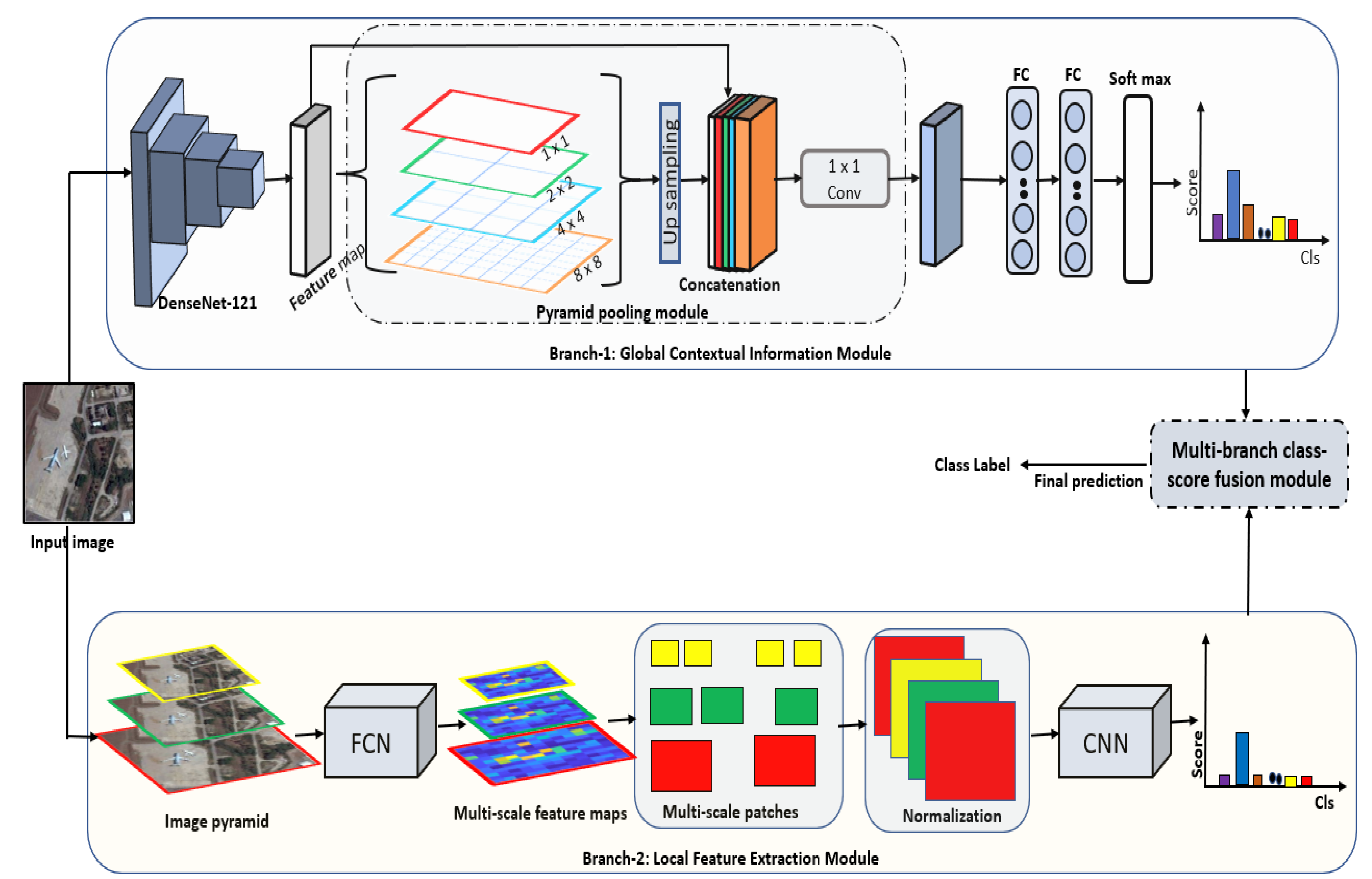
Unlike previous methods, the first branch of the framework (global contextual module) effectively aggregates contextual information from various regions of the images by integrating the pyramid pooling module.

3.

The local feature extraction module extracts multi-scale information and reduces background noise by learning discriminating features from the local regions of the image.

4.

We gauged the performance on three publicly available challenging datasets. From the experiments results, we demonstrate the effectiveness of the proposed framework.

We organize this paper as follows: Section 2 discusses the recent literature related to our work. We provide details of the proposed framework in Section 3. In Section 4, we provide the details of the datasets and present the comparison results with other reference methods. In Section 7, we discuss the significance of the proposed work, future work, and finally conclude the paper.

2. Related Work

In this section, we precisely review the related methods for land cover classification tasks proposed during the last decade. Generally, we divide these methods into two main categories: (a) unsupervised models and (b) supervised models. We further classify supervised methods into (1) handcrafted feature representation models and (2) deep hierarchical feature models.

2.1. Unsupervised Models

Unsupervised feature models automatically learn the features from unlabeled images. These models do not rely on learning manually designed features and can directly learn discriminating features from the raw images. Due to this unique property, these models have received much attention from the research community during recent years. Acknowledging the success of these models, the research community has tried to explore the benefits of these models for land cover classification tasks. An unsupervised feature learning method is proposed in [29] for scene classification in aerial images. The method learns a set of basis functions by extracting dense low-level feature descriptors to identify various spatial patterns in the scene. A two-layer sparse coding model is proposed in [30] that introduces visual attention to precisely identify image scenes by focusing more on saliency information and by relaxing the training phase. Similarly, a sparse coding method is used in [31] to extract local ternary pattern histogram Fourier (LTP-HF) and rotation-invariant texture features. These features are then combined, and a two-stage linear support vector machine is trained to classify scenes in high-resolution satellite images. An unsupervised feature learning model is proposed in [32] for satellite image retrieval based on collaborative matrix fusion. The framework extracts four various handcrafted texture features, including LBP, GLCM, SIFT, and MR8. The framework then fuses these features through an affinity metric. A spectral clustering algorithm is proposed in [33] that learns local features as well as inherent local structures of the image patches. The model adopts the manifold analysis method to project the patches of images to low-dimensional space and learns the dictionary by employing the K-means clustering algorithm that clusters similar features. Similarly, an unsupervised model is proposed in [34] that exploits the relationship between the intensity and color information. A two-layer unsupervised model is proposed in [35] that extracts edge and corner-like features from satellite images. The K-means clustering algorithm is adopted that jointly learns simple and complex structures in the satellite image. A saliency-guided unsupervised model is proposed in [36] for remote scene classification. The model extracts representative image patches from the salient regions of the image, and then, a set of features are learned through an unsupervised learning process.

Considering the task of scene classification in remote sensing images, unsupervised models suffer from the following limitations: (1) A large portion of unsupervised models rely on clustering techniques that require manual interpretations of different patterns. These manual interpretations lack the actual representation of the data due to which these models introduce biases and inconsistencies in the classification results. (2) Since these models are not trained on labeled data, these models have limited generalization and may not recognize and classify the new data. (3) These models focus on capturing the statistical features of the data and do not incorporate multi-scale contextual information that is crucial for such classification tasks.

2.2. Supervised Models

Generally, supervised models work in two stages. In the first stage, the model extracts features from the labeled data. In the second stage, a machine learning algorithm is employed to learn the features (extracted during the first stage) and predicts the output. Generally, we categorize these models into the following two categories:

2.2.1. Handcrafted Feature Representation Models

This class of models requires domain knowledge and heavily relies on the computation of complex features. These features include, edge, color, corner, texture, shape, size, and other complementary features required for scene classification.

In [37], the authors proposed an auto encoder–decoder model for scene classification in remote sensing images. The model learned a mid-level visual dictionary by learning discriminating visual features that capture high-level context of the image. The authors proposed a model [38] that quantizes non-spatial features and uses bag of visual words (BOVW) for land use classification problems. The model in [39] uses a color structure code (CSC) and support vector machine for land cover classification. A mutual information learning scheme is adopted in [40] to encode the structure of the given image using a local binary pattern (LBP). Rich texture information is captured via a multi-scale completed local binary pattern (CLBP) in [41], and kernel-based learning is adopted for land use classification tasks. The model in [42] identifies the statistical signature of the object by exploiting saliency information and GIST features. The saliency information extracts the local details of the object while the GIST features capture the global contextual features. Both of these features are combined, and a SVM model is trained to detect and classify the target in satellite images. A combination of Gabor and GIST descriptors is used in [43] for aerial image classification. The model computes Gabor and GIST features and then trains a support vector machine for aerial image classification. SIFT-based visual vocabulary is learned in [43] to classify complex scenes in remote sensing images. Texture and color information is exploited in [44], which decomposes a 2D discrete wavelet transform using bag of visual words for land cover classification. The method extracts local features from the grey-scale image and then decomposes the image into dense regions. The model then computes a histogram of visual words by computing visual words from dense regions. The model [45] extracts multi-scale, multi-resolution LBP features and local codebookless features from images. The combined model fuses both features and learns kernel-based extreme learning for classifying high-resolution satellite images.

Based on the discussion above, it is evident that handcrafted feature-based supervised models have been widely employed for scene classification in remote sensing. However, these models have several shortcomings and limitations that hinder their performance and applicability. (1) These models require domain expertise to manually design and extract features from remote sensing images. This process can be time-consuming and labor-intensive, and the selected features may not capture all the relevant information present in the data, leading to sub-optimal performance. (2) Since features are designed based on specific assumptions, these models have poor generalization capability. (3) The features engineered manually may fail to capture multi-scale information and contextual relationships adequately, resulting in diminished performance. (4) Handcrafted features are based on simplistic assumptions and may not comprehensively capture the intricate patterns and interactions among various objects or regions in the scene. (5) Handcrafted feature-based models may not properly utilize the spatial relationships between pixels and therefore face difficulties in capturing the spectral characteristics specific to different scene classes.

2.2.2. Deep Hierarchical Feature Models

In contrast to handcrafted features models, deep learning models learn deep hierarchical and powerful features from various layers of the network and efficiently discover context and structural features from multidimensional training data [46]. Due to the success of deep learning models, various networks have been designed to solve various problems in remote sensing applications. A deep learning framework is proposed in [47] that identifies various crop types in remote sensing images. A novel multi-scale deep learning framework is proposed in [48]. The framework employs an atrous spatial pyramid pooling (ASPP) module to extract multi-scale discriminating features and combines the advantages of two deep learning models ASPP-Unet and ResASPP-Unet for identifying different land cover in remote sensing images. A deep belief network (DBN) is proposed in [49] that combines the advantages of both supervised and unsupervised learning strategies. The framework extracts rich contextual features from synthetic aperture radar (SAR) data. In [50], the authors adopt a transfer learning strategy for land-scene classification in remote sensing images. The authors proposed two strategies of feature extraction. In the first strategy, the model extracts features from fully connected layers, and in the second strategy, the model uses the last convolutional layer for feature extraction and then employs various feature coding schemes. A multi-scale bag of visual words (MBVW) based on a deep learning feature framework is proposed in [51] for scene classification. A capsule network-based framework is proposed in [52] that uses a pretrained model for feature extraction. Then, the feature set is provided as input to the capsule network (CapsNet) to classify different scenes in remote sensing images. A comprehensive analysis of different deep learning models is proposed in [53] that utilizes different convolutional neural networks to understand the performance of these models in scene classification tasks in remote sensing images. A feature fusion model is proposed in [54] that employs the VGG-16 model to extract multi-scale features, and then, a fusion layer is introduced to fuse hierarchical features in four different branches. A similar fusion model is proposed in [55] that extracts features from various layers and then employs the Fisher kernel coding scheme to construct a mid-level representation of deep features. The framework fuses mid-level features and features of the last convolutional layer by principal component analysis that finally predicts the classification score of the given scene. A bag of convolutional features (BoCF) is proposed in [56] that generates visual words based on deep features. A graph convolutional network is proposed in [57] that integrates the deep features for scene classification in remote sensing images. A zero-shot learning model is proposed in [58] that classifies the unseen land cover scenes in high-resolution satellite images. A binary segmentation model for road extraction in high-resolution satellite images is proposed in [59] that employs statistical machine learning models, including decision trees, KNN, and SVM to classify the image into two classes. Similarly, an ensemble framework of SegNet and U-Net is proposed in [60] for building segmentation. A generative adversarial network (GAN) framework is proposed in [61] that employs SegNet with Bi-LSTM for building segmentation.

While the aforementioned methods have shown remarkable success in various semantic segmentation tasks for natural images, they fall short when applied to the scene classification task in remote sensing images. The limitations of existing models, such as CapsNet, U-Net, and VGG-16, in identifying a complex scene in aerial images are primarily due to their single-scale nature, which cannot adequately handle the wide range of variations in object scales and sizes. Consequently, these models fail to deliver satisfactory performance in capturing complex farmland patterns. In contrast, the proposed model addresses this issue by utilizing multiple branches, where branch-1 effectively integrates the pyramid pooling module that captures global contextual information from the scene, wile branch-2 of the framework extracts multi-scale features and captures local features. The proposed multi-branch architecture effectively identifies complex scenes with objects of different scales and sizes.

3. Methodology

Generally, the proposed framework is a multi-branch deep learning framework that consists of two deep learning branches. In the first branch, a deep learning network is responsible for extracting global contextual features from the input image, while the second branch extracts local information by identifying important regions in the input image. The framework then employs deep feature fusion module to fuse the classification scores of both branches and to obtain a classification final score for the input image. The parameters of the framework are optimized by a combined loss function. The overall architecture of the proposed framework is shown in Figure 2. We provide details of individual deep learning models as follows.

3.1. Branch-1: Global Contextual Information Module

The global contextual branch follows the pipeline of a traditional convolutional neural network. We use DenseNet [62] as a feature extractor in our global contextual branch. DenseNet has enjoyed tremendous success in various object classification, detection and segmentation tasks compared to other deep learning models. In traditional deep learning models, information passes through several convolutional and pooling layers connected via one-to-one connections. Due to a large number of layers and direct one-to-one connections among the layers, the information cannot reach to the last layers of the network that leads to the gradient vanishing problem. In contrast to one-to-one connections, each layer of the DenseNet utilizes feature maps from all previous layers and provides its own feature map to all subsequent layers. Such dense connections among the layers improve the information flow and avoid the gradient vanishing problem. Furthermore, parameters among the layers are efficiently shared, which leads to a lesser number of parameters to learn and which improves the convergence process during training.

We use DenseNet-121 in our global contextual branch that consists of 121 layers. Generally, the network consists of four dense blocks, $\{D_1,D_2,D_3,D_4\}$ and three transition layers, $\{T_1,T_2,T_3\}$.

The dense block $D_1$ consists of a stack of 6 × 2 = 12 convolutional layers. The second dense block $D_2$ consists of 12 × 2 = 24 layers, $D_3$ consists of 24 × 2 = 48 layers and last dense block $D_4$ consists of 16 × 2 = 32 convolutional layers. The three transition layers, $\{T_1,T_2,T_3\}$ are sandwiched between three dense blocks, $\{D_1,D_2,D_3\}$, and the size of the feature maps of each dense block is reduced by half after passing through the transition layers. The output feature maps of the last dense block $D_4$ is utilized by the classification layer in the original DenseNet architecture.

Although deep learning models achieve their best results in different classification tasks in natural images, their performance degrades due to the following reasons: (1) Aerial images are captured from a long-distance camera, where different objects appear similar and where it is hard for the deep learning model to extract discriminating features. (2) Multiple objects in high-resolution satellite images occupy small areas and adopt different sizes and shapes. It is challenging for a deep learning model with a fixed scale to extract multi-scale features. (3) Most of the existing classification models use the feature maps of the last convolutional layer for classification; for example, DenseNet-121 uses dense block $D_4$ for classification. Generally, the receptive field of such a deep learning network is large, and it is challenging for such networks to extract features of small objects and to capture rich context.

To remedy the aforementioned problems, we modify DenseNet-121 by integrating the pyramid pooling module adopted in PSPNet [63] for the semantic segmentation task. The pyramid pooling module accumulates rich context from various regions of the input feature map by employing sub-region average pooling operations of different sizes. In our framework, the feature map obtained from dense block $D_4$ is pooled at four different scales $\{1,2,4,8\}$. The first level is coarsest, where the feature map is pooled with 1 × 1 that converges all information of the feature map into a single bin. Similarly, at the subsequent levels, the feature map is divided into 2 × 2, 4 × 4 and 8 × 8 sub-regions, and then, average pooling operations are performed on each sub-region to obtain a respective pooled map. At lower levels (1–2), the network captures low-level features, while at higher levels (6–8), the network captures more contextual information. The pooled feature maps are concatenated with the original feature map (obtained from dense block $D_4$). For concatenation, the pooled feature maps are first upsampled by employing bi-linear interpolation to make the sizes equal to the size of the original feature map. Then, original and pooled feature maps are flattened, concatenated and fed to the fully connected layer for classification.

3.2. Branch-2: Local Feature Extraction Module

Th global contextual branch extracts useful information, for example, texture and contour from the whole image; however, local features are usually ignored. The receptive field of the global contextual branch is large and cannot capture information from local regions. Since local regions occupy a small portion in the whole image and are generally surrounded by a large background area, it is hard for the global contextual branch to extract local discriminating features.

To tackle this problem, we propose a two-stage model to extract discriminating features from important local areas of the input image. Generally, the model reasons about the location of important regions, extracts fine-grained features from the local regions, and suppresses background noise. Precisely, the local feature extraction branch consists of two deep learning networks: (1) the object proposal generation network and (2) the object proposal classification network. The first deep learning network extracts important regions (object proposals), and the second deep learning network is used to extract features from each important region and then classifies each proposal into a specific class.

An object proposal generation network is a data-driven deep learning network that reasons about as to what degree a particular region (in original image) contains an object or background. Generally, an object proposal generation network is a binary classifier that follows the pipeline of a fully convolutional network (FCN). It takes an arbitrarily sized image and outputs a dense heat map. Each pixel in the dense heat map shows the probability of the presence of an object in that particular region. To cover large variations in object scales, we first generate an image pyramid of different sizes and then provide each level of the pyramid to FCN as input. FCN generates multiple heat maps of different scales corresponding to different levels of the pyramid. We then employ a non-maximum suppression technique on all heat maps to suppress the low-confidence pixels and to obtain more refined heat maps. We then perform blob analysis to obtain multi-scale important regions/proposals.

For training the network, instead of using the whole image, we adopt patch-wise training. For patch-wise training, we extract several patches from the image and categorize those patches into two categories: object and background. For generating positive patches (corresponding to objects), we crop several patches around the object and compute the intersection over union (IoU) for each patch. Let $\mathbb{V}=\{p_1,p_2,\cdots ,p_n\}$ represent a set of n number of patches extracted from the training set of images. We labeled patch $p_i$ as positive sample for which IoU ≥ 0.5 or is a negative sample otherwise. Furthermore, for generating a negative patch (corresponding to the background), we randomly crop several patches from the background areas. We assign label 1 to the positive set of patches and 0 to the background patches. We assume that the image level ground truth is available for all images.

An object proposal classification model is a multi-class classification network that takes object proposals (generated by the objected proposal generation network) as input and classifies each proposal into a specific class. The network follows a similar pipeline of the object proposal generation network; however, instead of predicting binary labels, the network classifies the instances into predefined categories. For training the network, we use the same patch-wise training strategy as adopted for training the object proposal generation network; however, we assign class labels to each patch instead of binary labels.

3.3. Multi-Branch Class Score Fusion Module

In order to utilize global and local information from different branches of the framework, we use the prediction scores obtained from two branches. We assumed that most semantic classes are strongly associated with specific objects, for example, an airport can be effectively recognized by airplanes. Therefore, it is important to capture both global context and information about the local objects to precisely classify the given scene. To capture local and global characteristics of a given scene, we adopt a late fusion strategy [64] by averaging the prediction scores of two branches. There are several class score fusion strategies, including max fusion, average fusion, weighted fusion [65], voting fusion [66], stacking fusion [66], and concatenation fusion [67]. However, we use the average fusion strategy in our work due to the following reasons: (1) Average fusion helps to reduce the impact of outliers or noisy predictions from individual classifiers by taking the average of class scores, which smooths out individual fluctuations, resulting in a more reliable and robust prediction. (2) In complex classification problems, individual classifiers may generate slightly different predictions due to variations in their training or architecture, as in the case of the proposed framework that consists of two branches. Averaging the class scores helps to reduce the noise introduced by these slight differences, leading to a more stable and accurate overall prediction. (3) Averaging the class scores from multiple classifiers can be seen as an ensemble method. Ensemble methods aim to combine the predictions of multiple models to achieve better performance than any individual model. (4) Average fusion is a straightforward and easy-to-understand fusion strategy. It does not require additional parameters or complex operations, making it computationally efficient.

4. Experimental Results

To perform the experiments and to assess the performance of the proposed framework, we used a PC equipped with a Core i7 processor and 16 GB of RAM. The training process made use of the NVIDIA TITAN V GPU. The framework was implemented using the PyTorch library.

For training both branches, we used the pretrained models of widely use CNN networks, AlexNet [20], VGG16 [68], DenseNet [62], ZF [69], and GoogleNet [70] in our framework. Stochastic gradient descent (SGD) was used for training the network, and we used a learning rate of 0.001 that decreased by 1/10 after every 20 epochs. For both networks, we used a cross-entropy loss function to optimize the loss function. We trained the networks for 100 epochs with a batch size of 64. Before feeding the network with patch, each patch was re-sized (224 × 224) to fit the input of the network. We trained both networks of the local feature extraction branch independently.

We trained each branch of the framework independently. We used an image level training strategy to train branch-1 and used a patch-wise training strategy to train branch-2 of the framework. We first trained branch-1, as it extracts global information and provides a holistic view by assigning a scene classification score. We then trained branch-2 to provide scores based on important local regions. Finally, the two scores were fused together by employing a fusion block.

In the following sections, we first provide the details of the dataset. We then discuss the evaluation metrics and then provide the details of comparisons with existing related methods.

4.1. Datasets

The UC-Merced Dataset was proposed by Yang et al. [38] in 2010. The dataset consists of 21 different classes of aerial images, collected from 21 different locations in the United States. These locations include San Diego, Ventura, New York, Tucson, Napa, Buffalo, Seattle, Tampa, Boston, Santa Barbara, Jacksonville, Los Angeles, Miami, Dallas, Harrisburg, Birmingham, Houston, Columbus, Las Vegas, and Reno. Each category contain 100 images. The pixel resolution of each image is 256 × 256, and spatial resolution of each image is 30 cm per pixel. The images contain a variety of complex patterns with homogeneous and non-homogeneous textures and colors. Due to the complex nature of the dataset, this dataset has been widely used for evaluating different algorithms for land-use classification. We split the dataset into training and testing sets by following the same convention adopted in [71]. We kept 80% of the samples for training the framework, and the remaining 20% of samples were used for testing purposes. Sample frames from the UC-Merced dataset representing different classes are shown in Figure 3.

The SIRI-WHU dataset was first proposed by [72]. The dataset consists of 2400 satellite images collected from Google Earth and is categorized into 12 different classes that cover different urban areas in China. Each class contaisn 200 samples with a pixel resolution of 200 × 200 and spatial resolution of 2 m. The second column of Table 1 shows different classes of the dataset and their corresponding class labels. Sample frames from the SIRI-WHU dataset representing different classes are shown in Figure 4.

The EuroSAT dataset was proposed by Helber et al. [73] for land cover and land use classification tasks. The dataset contains ten classes and consists of 27,000 images collected in different cities from 34 European countries. The description of classes and their corresponding labels are provided in Table 1. The images were acquired from the Sentinel-2A satellite and cover complex land cover scenes with high intra-class variance. Each class of the dataset contains different land covers and contains 2000 to 3000 images per class. The pixel resolution of each image is 64 × 64, while the spatial resolution is 10 m per pixel. To further categorize the different agriculture land covers, the class is sub-divided into two classes, i.e., annual crop and permanent crop. Similarly, to differentiate different types of buildings and road footprints, the classes are divided into industrial and residential highway classes. Different configurations of the training test, for example, 10/90, 20/80, 30/70, etc., have been adopted to evaluate the performance of different models on the EuroSAT dataset. In this work, we used 80% of the data for training and the rest for testing. The comparison summary of the three datasets is provided in

Table 2. Summary of three datasets.

Dataset	UC Merced  [38]	SIRI-WHU  [38]	EuroSAT  [73]
No. of categories	21	12	10
Images per category	100	200	2000∼3000
Image size (pixels)	256 × 256	200 × 200	64 × 64
Spatial resolution (meters)	0.3	2	10
Total images	2100	2400	27,000
Train percentage	80	70	80
Test percentage	20	30	20

. Sample frames from the EuroSAT dataset representing different classes are shown in Figure 5.

Table 1. Categories and their corresponding class labels for three datasets.

Label	UC-Merced [38]	SIRI-WHU [72]	EuroSAT [73]
1	Agricultural	Agricultural	Annual Crop
2	Airplane	Commercial	Forest
3	Baseball diamond	Harbor	Herbaceous
4	Beach	Idle land	Highway
5	Buildings	Industrial	Industrial
6	Chaparral	Meadow	Pasture
7	Dense residential	Overpass	Permanent Crop
8	Forest	Park	Residential
9	Freeway	Pond	River
10	Golf course	Residential	Sea & Lake
11	Harbor	River	-
12	Intersection	Water	-
13	Medium-density residential	-	-
14	Mobile home park	-	-
15	Overpass	-	-
16	Parking lot	-	-
17	River	-	-
18	Runway	-	-
19	Sparse residential	-	-
20	Storage tanks	-	-
21	Tennis courts	-	-

Table 1. Categories and their corresponding class labels for three datasets.

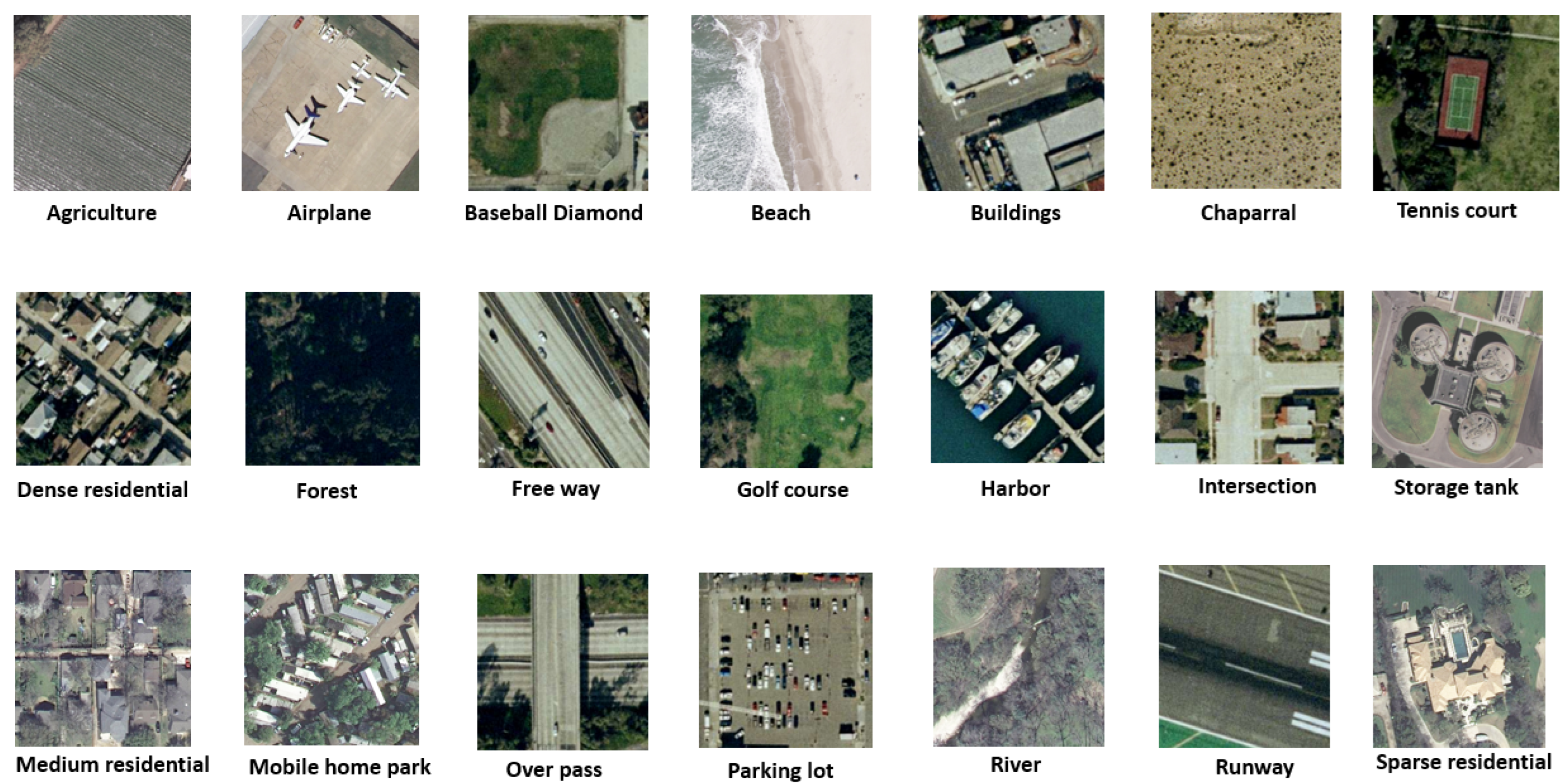
Label	UC-Merced [38]	SIRI-WHU [72]	EuroSAT [73]
1	Agricultural	Agricultural	Annual Crop
2	Airplane	Commercial	Forest
3	Baseball diamond	Harbor	Herbaceous
4	Beach	Idle land	Highway
5	Buildings	Industrial	Industrial
6	Chaparral	Meadow	Pasture
7	Dense residential	Overpass	Permanent Crop
8	Forest	Park	Residential
9	Freeway	Pond	River
10	Golf course	Residential	Sea & Lake
11	Harbor	River	-
12	Intersection	Water	-
13	Medium-density residential	-	-
14	Mobile home park	-	-
15	Overpass	-	-
16	Parking lot	-	-
17	River	-	-
18	Runway	-	-
19	Sparse residential	-	-
20	Storage tanks	-	-
21	Tennis courts	-	-

4.2. Evaluation Metrics

To quantitatively evaluate the proposed framework, we used common evaluation metrics. These metrics include overall accuracy (OA), confusion metric (CM), precision, recall, and F1 score. The details of all evaluation metrics are provided as follows:

• Overall accuracy (OA) measures and provides general insight about the performance of the framework and is computed as the ratio of the number of samples correctly classified to the total number of samples in the test set.
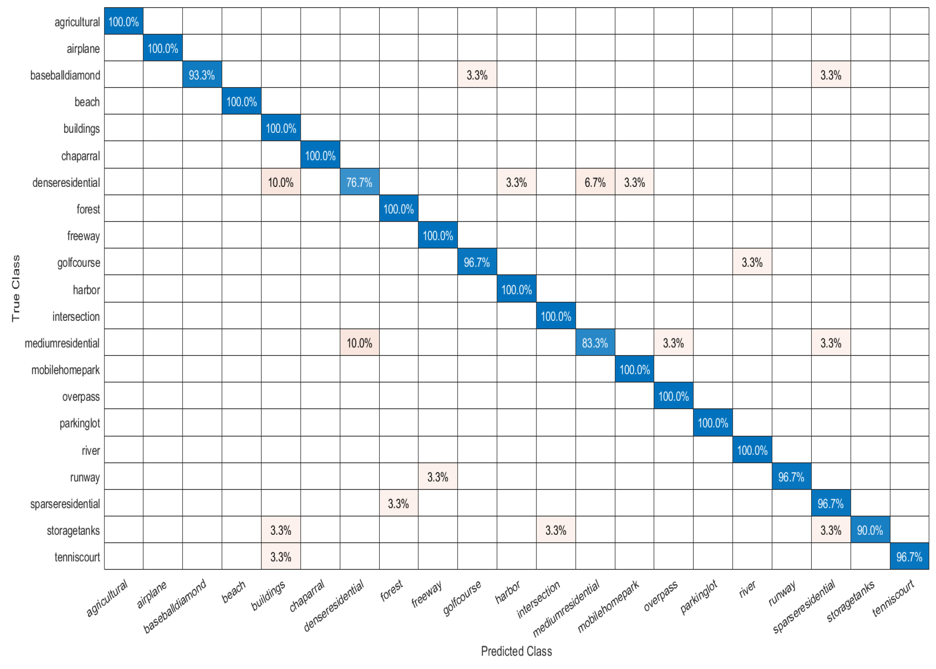
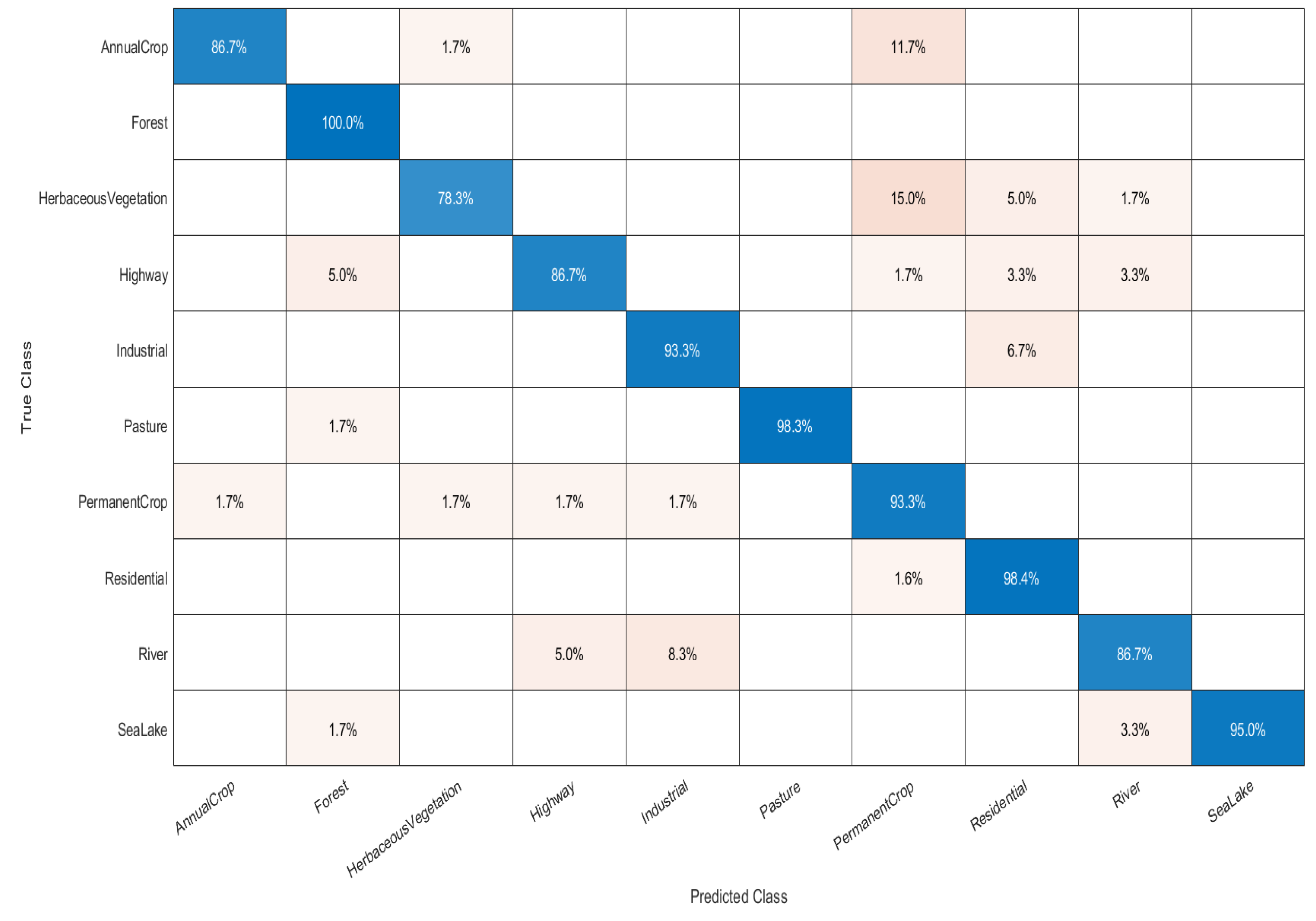
• The confusion matrix (CM) is a 2D matrix that gauges the detailed performance of classification models. The matrix measures the robustness of the models by computing inter-class and intra-class classification errors. Each row of the matrix represents the true class, while each column represents the predicted class. The value of each cell of the matrix gives insight into the degree of accuracy achieved by the classifier for a particular class.
• Precision, recall and F1 score are the popular metrics used to evaluate the performance of a classifier given the imbalanced data. Precision quantifies the ability of a model to precisely predict the class for the given samples that actually belong to the positive class. Precision can be measured as: $\frac{{\sum }_{i=1}^{C}T{P}_i}{{\sum }_{i=1}^C(T{P}_i+T{N}_i)}$, where C is the number of classes, and i represents the $i^{th}$ class. TP represents the true positive, and TN represents the true negative. The precision metric can be used to evaluate the performance of the model when the goal is to minimize the false positives.
• Recall, on the other hand, provides an indication to the missed positive prediction and can be mathematically expressed as: $\frac{{\sum }_{i=1}^{C}T{P}_i}{{\sum }_{i=1}^C(T{P}_i+F{N}_i)}$, where FN represents the false positive. The recall metric can be used as a performance measure where the goal of the model is to minimize the false negatives. The F1 score quantifies the performance of a model in a single metric by taking the harmonic mean of both precision and recall.

The classification performance in terms of the confusion matrix UC-Merced dataset using the proposed framework is reported in Figure 6. Furthermore, we report precision, recall and F1 score values for each individual class in

Table 3. Class-wise performance of the proposed framework on the UC-Merced dataset.

Class Name	Precision	Recall	F1 Score
Agricultural	100.00%	100.00%	100.00%
Airplane	100.00%	100.00%	100.00%
Baseball Diamond	100.00%	93.33%	96.55%
Beach	100.00%	100.00%	100.00%
Buildings	85.71%	100.00%	92.31%
Chaparral	100.00%	100.00%	100.00%
Dense Residential	88.46%	76.67%	82.14%
Forest	96.77%	100.00%	98.36%
Freeway	96.77%	100.00%	98.36%
Golf Course	96.67%	96.67%	96.67%
Harbor	96.77%	100.00%	98.36%
Intersection	96.77%	100.00%	98.36%
Medium Residential	92.59%	83.33%	87.72%
Mobile Home Park	96.77%	100.00%	98.36%
Overpass	96.77%	100.00%	98.36%
Parking Lot	100.00%	100.00%	100.00%
River	96.77%	100.00%	98.36%
Runway	100.00%	96.67%	98.31%
Sparse Residential	90.63%	96.67%	93.55%
Storage Tanks	100.00%	90.00%	94.74%
Tennis Court	100.00%	96.67%	98.31%

. We can see from the Figure 6 that the proposed framework achieved 100% classification accuracy in 11 different categories, while in 6 categories, the framework achieved a ≥ 90% classification accuracy. Similarly, as demonstrated in Table 3, the proposed framework achieves 100% precision, recall and F1 score values in five different classes, while for the remaining class, the proposed framework achieves more than 90% precision, recall and F1 score.

The classification performance of the proposed framework in terms of the confusion matrix on the SIRI-WHU Dataset is reported in Figure 7, and precision, recall, and F1 score values for each individual class are reported in

Table 4. Class-wise performance of the proposed framework on the Siri-WHU dataset.

Class Name	Precision	Recall	F1 Score
Agriculture	100.00%	100.00%	100.00%
Commercial	93.65%	98.33%	95.93%
Harbor	92.31%	100.00%	96.00%
Idle Land	93.10%	90.00%	91.53%
Industrial	98.33%	98.33%	98.33%
Meadow	91.23%	86.67%	88.89%
Overpass	100.00%	100.00%	100.00%
Park	88.71%	91.67%	90.16%
Pond	90.32%	93.33%	91.80%
Residential	92.06%	96.67%	94.31%
River	90.57%	80.00%	84.96%
Water	100.00%	95.00%	97.44%

. From Figure 7, it is obvious that the framework achieves more than 95% accuracy in seven different categories. In addition, the framework achieved more than 90% accuracy in three classes. Similarly, from Table 4, we observe that the proposed framework achieves 100% precision, recall and F1 score values for the agriculture and overpass classes, while the framework achieves more than 90% precision, recall rate and F1 score values for seven classes, including, commercial, harbor, idle land, industrial, pond, residential, and water.

Figure 8 illustrates the confusion matrix, and

Table 5. Class-wise performance of the proposed framework on the Eurosat dataset.

Class Name	Precision	Recall	F1-Score
Annual Crop	98.11%	86.67%	92.04%
Forest	92.31%	100.00%	96.00%
Herbaceous Vegetation	95.92%	78.33%	86.24%
Highway	92.86%	86.67%	89.66%
Industrial	90.32%	93.33%	91.80%
Pasture	100.00%	98.33%	99.16%
Permanent Crop	75.68%	93.33%	83.58%
Residential	86.96%	98.36%	92.31%
River	91.23%	86.67%	88.89%
Sea Lake	100.00%	95.00%	97.44%

illustrates the performance of the framework using precision, recall and F1 score on the EuroSAT dataset. Figure 8 shows that the proposed framework achieved more than 93% accuracy in six classes, while the framework achieved 86% accuracy in three classes. Similarly, the framework achieved more than 90% precision, recall and F1 score values for the our classes, including, forest, industrial, pasture, and sea lake.

We also visualized the performance of the proposed framework through random sampling frames from all three datasets, with each sample displaying both the ground truth label and the predicted label as illustrated in Figure 9. From the Figure 9, it is also obvious that the proposed framework precisely predicted all the labels of different classes; however, the model was confused regarding herbaceous vegetation and permanent crop classes.

In Table 6, we compare the performance of different methods on three datasets and their overall accuracy (OA) evaluation measure. For fair comparisons, we used the same training and testing ratios for all the methods. From Table 5, it is observed that the proposed framework achieves better results compared to other referenced methods.

From Table 6, it is obvious that the models, including NSGA-II, MOEA, AR-MOEA, and SMS-EMOA, achieve lower performance compared to other competing methods. In [74], the authors use the pretrained model of ResNet-50 and adopt different pruning strategies, including NSGA-II, MOEA, AR-MOEA, and SMS-EMOA, to compress and accelerate the network. The basic intuition behind compressing the high-capacity networks is to minimize the weights without compromising the accuracy and to make these networks suitable for the platform with limited memory and computational power. In the EMOA method, the pretrained model of ResNet-50 is pruned by evolutionary multiobjective algorithms, and it employs a guided mechanism and uses an indicator to find an optimum solution. Similarly, SMS-EMOA models prune the fine-tuned model of ResNet-50 by using a selection optimization algorithm. In AR-MOEA, the pretrained network of ResNet-50 is optimized with a reference point adoption strategy. NSGA-II adopts a sorting genetic algorithm to optimize the parameters of a pretrained ResNet-50. Although these models largely reduce the capacity of the network, they do so at the cost of accuracy. This is due to fact that after the pruning process, the network loses contextual and multi-scale information regarding small objects, which is crucial for scene classification in satellite images. Although EfficientNet demonstrated an effective performance compared to MobileNet [75] and ResNet [76] in natural images, from our experiments, we observe that EfficientNet achieves low performance in satellite images. This may be attributed to the complex texture, cluttered background, small size of objects, and high inter-class similarities among different patterns of satellite images, which do not fit the EfficientNet and do not achieve a comparable performance. From Table 6, we observe that SKAL [22] achieves a comparable performance on the UC-Merced dataset. This may be attributed to the fact that SKAL employs multi-branch deep learning models that have the ability to exploit the complementary nature of different models, which effectively captures the local and global information from the images.

From Table 6, we further observe that the baseline architectures of ResNet-50 and ResNet-101 also achieve comparable performance on all three datasets. Although the inclusion of residual connections on ResNet gives a boost to the learning ability of the network and overcomes the gradient vanishing problem, the network achieves comparatively low performance on satellite images. This may be attributed to the fact that the receptive field of ResNet is higher than the size of the input image and therefore cannot capture information about the local regions that usually lead to the misclassification of pixels. In contrast to these competing methods, the proposed framework achieves superior results in all three datasets. This is due to the reason that the global contextual module of the framework extracts information in a global context, while the local feature extraction module extracts the features of local regions.

Table 6. Comparisons of different methods on the three datasets.

Method	Overall Accuracy
	UC Merced	Siri-WHU	Eurosat
EfficientNet [77]	88.00%	83.88%	85.23%
Wang et al. [78]	94.81 %	-	-
MobileNet [75]	93.00%	92.63%	87.52%
NSGA-II [79]	79.17%	72.14%	-
ResNet-50 [76]	95.00%	93.75%	90.34%
MOEA [80]	79.23%	71.98%	-
ResNet-101 [76]	95.00%	93.14%	90.51%
Yang et al. [81]	93.67%	-	-
AR-MOEA [82]	79.11%	72.34%	-
ShuffleNet [83]	91.00%	92.08%	88.68%
Basha et al. [84]	88%	-	-
SMS-EMOA [85]	78.45%	73.02%	-
Shao et al. [86]	92.38%	-	-
GoogleNet [70]	94.00%	91.11%	88.51%
SKAL [22]	97.95%	-	-
Proposed (Branch-1: DenseNet, Branch-2: VGG-16)	96.00%	94.16%	91.68%
Proposed (Branch-1: DenseNet, Branch-2: DenseNet)	99.52%	96.37%	94.75%

Table 6. Comparisons of different methods on the three datasets.

Method	Overall Accuracy
	UC Merced	Siri-WHU	Eurosat
EfficientNet [77]	88.00%	83.88%	85.23%
Wang et al. [78]	94.81 %	-	-
MobileNet [75]	93.00%	92.63%	87.52%
NSGA-II [79]	79.17%	72.14%	-
ResNet-50 [76]	95.00%	93.75%	90.34%
MOEA [80]	79.23%	71.98%	-
ResNet-101 [76]	95.00%	93.14%	90.51%
Yang et al. [81]	93.67%	-	-
AR-MOEA [82]	79.11%	72.34%	-
ShuffleNet [83]	91.00%	92.08%	88.68%
Basha et al. [84]	88%	-	-
SMS-EMOA [85]	78.45%	73.02%	-
Shao et al. [86]	92.38%	-	-
GoogleNet [70]	94.00%	91.11%	88.51%
SKAL [22]	97.95%	-	-
Proposed (Branch-1: DenseNet, Branch-2: VGG-16)	96.00%	94.16%	91.68%
Proposed (Branch-1: DenseNet, Branch-2: DenseNet)	99.52%	96.37%	94.75%

5. Ablation Study

We performed an ablation study to understand the effects of different components of the proposed framework on the overall accuracy. Conducting this ablation study was crucial for understanding and improving the performance of the framework. This study enabled us to make informed decisions to enhance the model’s accuracy and efficiency. In this ablation study, we employed the UC-Merced dataset and applied consistent training and validation strategies.

5.1. Ablation Study for Branch-1

To understand the effect of the pyramid pooling module with different pooling sizes, we performed an ablation study, as reported in Figure 7. We used seven different methods with different settings, and the performance of these methods are reported in

Table 7. Performance investigation of the effect of pyramid pooling module (in the global contextual information module (Branch-1)) with different backbone networks and different pooling scale settings on the UC-Merced dataset.

Method	Branch-1 Network	Branch-2 Network	Pooling Size	Pooling Type	OA
M1	DenseNet [62]	VGG-16 [68]	-	-	89.95%
M2			1 × 1	Max pooling	91.64%
M3			1 × 1	Avg pooling	92.74%
M4			[1 × 1, 2 × 2, 4 × 4, 8 × 8]	Max pooling	95.28%
M5 (proposed)			[1 × 1, 2 × 2, 4 × 4, 8 × 8]	Avg pooling	96.00%
M6 (proposed)		DenseNet [62]	[1 × 1, 2 × 2, 4 × 4, 8 × 8]	Max pooling	97.89%
M7 (proposed)			[1 × 1, 2 × 2, 4 × 4, 8 × 8]	Avg pooling	99.52%

. Each method is described as follows:

1.

Method M1: This method employs DenseNet in the Branch-1 network without a pyramid pooling module and VGG-16 in the Branch-2 network.

2.

Method M2: This method utilizes DenseNet in the Branch-1 network with a pyramid module comprising a single max-pooling layer of size 1 × 1, while VGG-16 is employed in Branch-2 network.

3.

Method M3: This method is similar to Method M2; however, instead of the max-pooling operation, the method employs an average pooling operation of size 1 × 1.

4.

Method M4: This method employs DenseNet in the Branch-1 network and employs the pyramid pooling module with four different pooling sizes. The model employs 1 × 1, 2 × 2, 4 × 4, 8 × 8 pooling with max-pooling and uses VGG-16 as the backbone of the Branch-2 network.

5.

Method M5 (proposed): This method is similar to Method M4; however, instead of using the max-pooling operation, it uses average pooling operations of sizes 1 × 1, 2 × 2, 4 × 4, 8 × 8.

6.

Method M6 (proposed): This method is similar to Method M4; however, it uses DenseNet as the backbone in Branch-2.

7.

Method M7 (proposed): This method is similar to Method M6; however, it employs average pooling operations instead of max-pooling.

By systematically analyzing and comparing different methods listed in Table 7, we can identify the impact of various components and design choices on the model’s performance. From Table 7, it is obvious that the methods M4, M5, M6, and M7 perform better than M1, M2, and M3. This is because methods M4, M5, M6, and M7 employ a pyramid pooling module by incorporating pooling layers of different sizes (1 × 1, 2 × 2, 4 × 4, 8 × 8). The pyramid pooling module captures multi-scale contextual information, enabling the model to extract features at various levels of granularity. By incorporating information from different receptive fields, the model gains a better understanding of global and local image features, resulting in improved performance compared to methods without the pyramid pooling module.

From Table 7, we further observed that methods M3, M5, and M7 utilize average pooling, producing better results than methods M2, M4, and M6, which utilize the max-pooling operation. The average pooling operation calculates the average value within a pooling window, which helps in preserving spatial information and reducing the impact of outliers. In contrast, the max-pooling operation selects the maximum value, which focuses on capturing the most dominant features. In this scenario, the average pooling operation performs better because it can retain more information and provide a smoother representation of features, leading to enhanced performance in the given deep model.

From Table 7, we observe that DenseNet is consistently employed in the Branch-1 network across multiple methods, while VGG-16 is used in methods M1, M2, M3, and M4. Methods M6 and M7 in Table 7 incorporate DenseNet in both the Branch-1 and Branch-2 networks, which achieve the highest overall accuracies (OA) of 97.89% and 99.52%, respectively, compared to M5, which employs VGG-16 in Branch-2. The lower performance of methods M1, M2, M3, and M4 is because VGG-16 relies on a deeper stack of convolutional layers without direct connections between them, which may limit information propagation and result in reduced performance compared to DenseNet. In contrast to VGG-16, DenseNet in both branches allows for the exploitation of dense connectivity and feature reuse across the entire network. This enables effective information flow and collaborative learning between the two branches. DenseNet’s dense connections facilitate the exchange of information, gradients, and feature maps between layers, enhancing the model’s capacity to capture discriminating patterns and to extract rich representations from the data.

5.2. Ablation Study for Branch-2

An efficient object proposal generation strategy helps to narrow down the search space for the objects in images and focuses on relevant areas, thereby significantly reducing the computational burden. The choice of the object proposal generation strategy can greatly influence the overall performance of a system. A well-designed strategy should be able to accurately localize objects, handle object scale variations, handle occlusions and cluttered backgrounds, and be computationally efficient.

Branch-2 of the proposed framework utilizes an object proposal generation strategy by employing a multi-scale fully convolutional network. In order to evaluate the impact of various object proposal generation strategies and different network configurations, an ablation study was conducted. This study, represented in Figure 8, aimed to systematically analyze and understand the effects of different approaches. By conducting this study, we can gain insights into the effectiveness and contributions of different strategies and networks.

Table 8. Performance investigation of local feature extraction module (Branch-2) using different region proposal strategies with different backbone networks on the UC-Merced dataset.

Region Proposal Strategy	Branch-2 Network	Overall Accuracy
RPN [88]	VGG16	93.45%
	ZF	92.98%
	AlexNet	87.63%
Selective Search [89]	VGG16	86.85%
	ZF	83.92%
	AlexNet	79.24%
Multibox [90]	VGG16	92.71%
	ZF	87.22%
	AlexNet	84.26%
Multiscale (Proposed)	VGG16	96.00%
	DenseNet (Avg pooling)	99.52%
	ZF	94.75%
	AlexNet	88.95%

presents the performance of the local feature extraction module (Branch-2) using different region proposal strategies with different backbone networks on the UC-Merced dataset. We used different networks as the backbone of Branch-2, including VGG-16 [68], ZF [69], and AlexNet [87]. From Table 8, it is obvious that the proposed multi-scale strategy achieved the best results compared to other region proposal strategies. This is because the proposed region proposal strategy enhances the adaptability of the object-detection system to objects of various scales and aspect ratios, resulting in improved accuracy. Furthermore, the combination of the proposed multiscale strategy and the DenseNet network leverages the strengths of both approaches, leading to superior performance in terms of overall accuracy on the UC-Merced dataset. Regarding the effect of different networks in Branch-2, we observed that VGG16 consistently achieves higher overall accuracy compared to ZF and AlexNet. This can be attributed to the architectural differences between these networks. VGG16 has a deeper architecture with more convolutional layers, allowing it to capture more complex and abstract features from the input images. The deeper representation of VGG16 enables better discrimination of object classes, resulting in higher accuracy in object detection. Selective search consistently achieves lower overall accuracy compared to other region proposal strategies across all backbone networks. Selective search is an algorithm that generates object proposals based on low-level image cues such as color, texture, and size. While it provides a diverse set of proposals, it may not capture high-level semantic information effectively. This limitation leads to the generation of more false positives or missed relevant object proposals, resulting in reduced accuracy compared to other strategies.

6. Discussion

In this section, we discuss the findings of the experimental results reported in Table 3, Table 4, Table 5 and Table 6. From the experimental results reported in Table 3, Table 4 and Table 5, we observe that the network achieved good performance in all three datasets; however, the network achieved the best results in the UC-Merced dataset. The best performance may be attributed to high inter-class differences and high intra-class similarities among these classes. This enabled the framework to correctly recognize these categories with ease. We further observed that the proposed framework is rotation- and scale-invariant and can recognize categories with different scales and orientations. From the experiments, we observed that the proposed framework outperforms other reference methods. From Table 6, it is observed that for the UC-Merced dataset, the framework achieved an overall accuracy of 96%. From the experimental results, we observed that ResNet-50 and ResNet-101 produced comparable results on all three datasets. However, there is no obvious difference between the performance of ResNet-50 and ResNet-101. From this study, we can superficially conclude that increasing the depth of the network by including more layers may not necessarily boost the performance by a significant margin regarding aerial images. We further observed that deeper layers may lead the network to learn discriminating features in natural images; however, these deep models do not perform well in aerial scenes [91].

We further observed that the reference methods achieved lower precision, recall and F1 score values for the EuroSAT dataset than on the UC-Merced and SIRI-WHU datasets. This finding is evident from Table 5. The lower performance on the EuroSAT dataset is attributed to the fact that it contains more diverse scenes and inter-class similarities among the annual crop, permanent crop and herbaceous classes. Due to these problems, the models are not able to learn discriminating features.

Despite demonstrating good performance on challenging datasets, the framework also suffers from limitations. From the experimental results, we observed that the network faces difficulties in differentiating between two similar images with two different classes. This inter-class similarity among different classes causes the network to learn similar features that leads the framework to misclassification. In the UC-Merced dataset, despite good performance, the framework achieved low performance (76%) accuracy in the dense residential class as illustrated in Figure 6 and Table 3. This is due to the fact that the framework confuses dense residential class with the buildings class by up to 10%, as well as 3.3% with harbor, 6.7% with medium residential and 3.3% with mobile home park classes. This may be because the dense residential class shares common textural and appearance features with the medium residential and building classes. Similarly, in the SIRI-WHU dataset, the framework, confuses the water class with pond, idle land, and harbor classes. We observed that a large number of river class images consist of idle land; therefore, the framework misclassifies most images of the river class in the test set. Similarly, the river class shares common features with the pond and harbor classes, and the framework faces difficulty in correctly classifying images from the river class. In the EuroSAT dataset, the framework achieved low performance while identifying the herbaceous vegetation class. The network largely confuses the herbaceous vegetation class with the permanent crop class, since both classes share similar appearance and morphological features.

Time Complexity

In this section, we provide detail of the time complexity of the proposed framework and compare its performance with other reference methods. Analyzing the time complexity of a deep learning model is crucial in understanding its efficiency and performance. Time complexity refers to the measure of the computational resources, specifically the time required for training the network and making predictions during inference.

In order to assess the computational complexity, we ensured consistency by using the same training parameters across all reference models. These models are then trained for 100 epochs, allowing us to compare and evaluate their computational demands accurately. Typically, the training phase of a network requires a longer duration, often measured in hours, compared to the much shorter testing time during the inference or prediction phase, which is typically measured in seconds. In this analysis, we utilized the UC-Merced dataset and present the findings in

Table 9. Time complexity of different models. Training time is given in hours, while testing time is provided in seconds.

Methods	Training Time (Hours)	Testing Time (Seconds)
DenseNet-baseline	10.20	3.35
ResNet-101	8.40	3.22
MobileNet	4.35	0.33
EfficientNet	12.50	3.15
GoogleNet	5.30	1.33
Proposed (Branch-1: DenseNet, Branch-2: VGG-16)	14.37	4.15
Proposed (Branch-1: DenseNet, Branch-2: DenseNet)	19.40	5.32

.

From Table 9, it is obvious that the methods MobileNet and GoogleNet have relatively shorter training times of 4.35 and 5.30 h, respectively. This is because these models are designed to be computationally efficient with lighter architectures, enabling faster training. On the other hand, we can observe that the method “Proposed (Branch-1: DenseNet, Branch-2: DenseNet)” has the highest training time of 19.40 h. This is because the proposed method involves using two DenseNet models in parallel (one for each branch). DenseNet models have a larger number of layers and parameters compared to other models such as ResNet-101, MobileNet, and GoogleNet. Despite the fact that the proposed framework takes longer for both training and inference compared to other methods, it outperforms them in terms of performance on all datasets. Therefore, the trade-off between longer training and inference times and improved performance justifies the adoption of the proposed framework in image classification in remote sensing images, where high accuracy is of utmost importance.

7. Conclusions

In this paper, a multi-branch deep learning framework was designed to identify different land scenes in complex remote sensing images. The framework consisted of two branches: (1) a global contextual module and (2) a local feature extraction module. The global module efficiently integrated the pyramid pooling module with DenseNet to capture rich contextual features from different regions of the image. The second module exploited FCN and CNN to extract multi-scale local features. The module first generated region proposals with FCN and then employed a CNN network to extract multi-scale features from each proposal. Later on, a fusion module was used to combine both local and global features to identify different land scenes. We demonstrated through comprehensive quantitative and qualitative evaluations that the proposed method achieves the best performance and outperforms other state-of-the-art methods. Despite good performance, the proposed framework still suffers from shortcomings. We observed that the framework faces difficulties in identifying two similar regions belonging to different classes. In future work, we will focus on rectifying the shortcomings of the proposed framework. Intuitively, we will extract feature embeddings and try to learn the distance between feature embeddings of different classes using a metric learning strategy. We believe that this may enhance the discriminating capability of the proposed framework.

References

- Dong, Z.; Wang, M.; Wang, Y.; Zhu, Y.; Zhang, Z. Object detection in high resolution remote sensing imagery based on convolutional neural networks with suitable object scale features. IEEE Trans. Geosci. Remote Sens. 2019, 58, 2104–2114. [Google Scholar] [CrossRef]
- Bastani, F.; He, S.; Abbar, S.; Alizadeh, M.; Balakrishnan, H.; Chawla, S.; Madden, S.; DeWitt, D. Roadtracer: Automatic extraction of road networks from aerial images. In Proceedings of the IEEE Conference on Computer Vision and Pattern Recognition, Salt Lake City, UT, USA, 18–22 June 2018; pp. 4720–4728. [Google Scholar]
- Khan, S.D.; Alarabi, L.; Basalamah, S. Deep Hybrid Network for Land Cover Semantic Segmentation in High-Spatial Resolution Satellite Images. Information 2021, 12, 230. [Google Scholar] [CrossRef]
- Talukdar, S.; Singha, P.; Mahato, S.; Pal, S.; Liou, Y.A.; Rahman, A. Land-use land-cover classification by machine learning classifiers for satellite observations—A review. Remote Sens. 2020, 12, 1135. [Google Scholar] [CrossRef]
- Khan, S.D.; Alarabi, L.; Basalamah, S. An Encoder–Decoder Deep Learning Framework for Building Footprints Extraction from Aerial Imagery. Arab. J. Sci. Eng. 2022, 48, 1273–1284. [Google Scholar] [CrossRef]
- Chiu, M.T.; Xu, X.; Wei, Y.; Huang, Z.; Schwing, A.G.; Brunner, R.; Khachatrian, H.; Karapetyan, H.; Dozier, I.; Rose, G.; et al. Agriculture-vision: A large aerial image database for agricultural pattern analysis. In Proceedings of the IEEE/CVF Conference on Computer Vision and Pattern Recognition, Seattle, WA, USA, 13–19 June 2020; pp. 2828–2838. [Google Scholar]
- Khan, S.D.; Alarabi, L.; Basalamah, S. A unified deep learning framework of multi-scale detectors for geo-spatial object detection in high-resolution satellite images. Arab. J. Sci. Eng. 2021, 47, 9489–9504. [Google Scholar] [CrossRef]
- Lin, L.; Di, L.; Zhang, C.; Guo, L.; Di, Y. Remote Sensing of Urban Poverty and Gentrification. Remote Sens. 2021, 13, 4022. [Google Scholar] [CrossRef]
- Kazemzadeh-Zow, A.; Darvishi Boloorani, A.; Samany, N.N.; Toomanian, A.; Pourahmad, A. Spatiotemporal modelling of urban quality of life (UQoL) using satellite images and GIS. Int. J. Remote Sens. 2018, 39, 6095–6116. [Google Scholar] [CrossRef]
- Hoque, M.A.A.; Phinn, S.; Roelfsema, C.; Childs, I. Tropical cyclone disaster management using remote sensing and spatial analysis: A review. Int. J. Disaster Risk Reduct. 2017, 22, 345–354. [Google Scholar] [CrossRef]
- Zhao, B.; Dai, Q.; Zhuo, L.; Zhu, S.; Shen, Q.; Han, D. Assessing the potential of different satellite soil moisture products in landslide hazard assessment. Remote Sens. Environ. 2021, 264, 112583. [Google Scholar] [CrossRef]
- Murray, N.J.; Keith, D.A.; Bland, L.M.; Ferrari, R.; Lyons, M.B.; Lucas, R.; Pettorelli, N.; Nicholson, E. The role of satellite remote sensing in structured ecosystem risk assessments. Sci. Total. Environ. 2018, 619, 249–257. [Google Scholar] [CrossRef]
- Mahato, S.; Pal, S. Groundwater potential mapping in a rural river basin by union (OR) and intersection (AND) of four multi-criteria decision-making models. Nat. Resour. Res. 2019, 28, 523–545. [Google Scholar] [CrossRef]
- Raeva, P.L.; Šedina, J.; Dlesk, A. Monitoring of crop fields using multispectral and thermal imagery from UAV. Eur. J. Remote Sens. 2019, 52, 192–201. [Google Scholar] [CrossRef]
- Yu, J.; Guo, P.; Chen, P.; Zhang, Z.; Ruan, W. Remote sensing image classification based on improved fuzzy c-means. Geo-Spat. Inf. Sci. 2008, 11, 90–94. [Google Scholar] [CrossRef]
- Wu, H.; Liu, B.; Su, W.; Zhang, W.; Sun, J. Hierarchical coding vectors for scene level land-use classification. Remote Sens. 2016, 8, 436. [Google Scholar] [CrossRef]
- Tuia, D.; Volpi, M.; Dalla Mura, M.; Rakotomamonjy, A.; Flamary, R. Automatic feature learning for spatio-spectral image classification with sparse SVM. IEEE Trans. Geosci. Remote Sens. 2014, 52, 6062–6074. [Google Scholar] [CrossRef]
- Stumpf, A.; Kerle, N. Object-oriented mapping of landslides using Random Forests. Remote Sens. Environ. 2011, 115, 2564–2577. [Google Scholar] [CrossRef]
- Moustakidis, S.; Mallinis, G.; Koutsias, N.; Theocharis, J.B.; Petridis, V. SVM-based fuzzy decision trees for classification of high spatial resolution remote sensing images. IEEE Trans. Geosci. Remote Sens. 2011, 50, 149–169. [Google Scholar] [CrossRef]
- Krizhevsky, A.; Sutskever, I.; Hinton, G.E. Imagenet classification with deep convolutional neural networks. In Proceedings of the Advances in Neural Information Processing Systems 25 (NIPS 2012), Lake Tahoe, NV, USA, 3–6 December 2012; p. 25. [Google Scholar]
- Anwar, A.; Anwar, H.; Anwar, S. Towards Low-Cost Classification for Novel Fine-Grained Datasets. Electronics 2022, 11, 2701. [Google Scholar] [CrossRef]
- Wang, Q.; Huang, W.; Xiong, Z.; Li, X. Looking closer at the scene: Multiscale representation learning for remote sensing image scene classification. IEEE Trans. Neural Netw. Learn. Syst. 2020, 33, 1414–1428. [Google Scholar] [CrossRef]
- Liang, G.; Hong, H.; Xie, W.; Zheng, L. Combining convolutional neural network with recursive neural network for blood cell image classification. IEEE Access 2018, 6, 36188–36197. [Google Scholar] [CrossRef]
- Ding, Y.; Zhang, Z.; Zhao, X.; Hong, D.; Cai, W.; Yu, C.; Yang, N.; Cai, W. Multi-feature fusion: Graph neural network and CNN combining for hyperspectral image classification. Neurocomputing 2022, 501, 246–257. [Google Scholar] [CrossRef]
- Ciregan, D.; Meier, U.; Schmidhuber, J. Multi-column deep neural networks for image classification. In Proceedings of the 2012 IEEE Conference on Computer Vision and Pattern Recognition, Providence, RI, USA, 16–21 June 2012; pp. 3642–3649. [Google Scholar]
- Nanni, L.; De Luca, E.; Facin, M.L.; Maguolo, G. Deep learning and handcrafted features for virus image classification. J. Imaging 2020, 6, 143. [Google Scholar] [CrossRef] [PubMed]
- Sandoval, C.; Pirogova, E.; Lech, M. Two-stage deep learning approach to the classification of fine-art paintings. IEEE Access 2019, 7, 41770–41781. [Google Scholar] [CrossRef]
- Xu, K.; Huang, H.; Deng, P. Remote sensing image scene classification based on global–local dual-branch structure model. IEEE Geosci. Remote Sens. Lett. 2021, 19, 1–5. [Google Scholar] [CrossRef]
- Cheriyadat, A.M. Unsupervised feature learning for aerial scene classification. IEEE Trans. Geosci. Remote Sens. 2013, 52, 439–451. [Google Scholar] [CrossRef]
- Dai, D.; Yang, W. Satellite image classification via two-layer sparse coding with biased image representation. IEEE Geosci. Remote Sens. Lett. 2010, 8, 173–176. [Google Scholar] [CrossRef]
- Sheng, G.; Yang, W.; Xu, T.; Sun, H. High-resolution satellite scene classification using a sparse coding based multiple feature combination. Int. J. Remote Sens. 2012, 33, 2395–2412. [Google Scholar] [CrossRef]
- Li, Y.; Zhang, Y.; Tao, C.; Zhu, H. Content-based high-resolution remote sensing image retrieval via unsupervised feature learning and collaborative affinity metric fusion. Remote Sens. 2016, 8, 709. [Google Scholar] [CrossRef]
- Hu, F.; Xia, G.S.; Wang, Z.; Huang, X.; Zhang, L.; Sun, H. Unsupervised feature learning via spectral clustering of multidimensional patches for remotely sensed scene classification. IEEE J. Sel. Top. Appl. Earth Obs. Remote Sens. 2015, 8, 2015–2030. [Google Scholar] [CrossRef]
- Risojević, V.; Babić, Z. Unsupervised quaternion feature learning for remote sensing image classification. IEEE J. Sel. Top. Appl. Earth Obs. Remote Sens. 2016, 9, 1521–1531. [Google Scholar] [CrossRef]
- Li, Y.; Tao, C.; Tan, Y.; Shang, K.; Tian, J. Unsupervised multilayer feature learning for satellite image scene classification. IEEE Geosci. Remote Sens. Lett. 2016, 13, 157–161. [Google Scholar] [CrossRef]
- Zhang, F.; Du, B.; Zhang, L. Saliency-guided unsupervised feature learning for scene classification. IEEE Trans. Geosci. Remote Sens. 2014, 53, 2175–2184. [Google Scholar] [CrossRef]
- Cheng, G.; Zhou, P.; Han, J.; Guo, L.; Han, J. Auto-encoder-based shared mid-level visual dictionary learning for scene classification using very high resolution remote sensing images. IET Comput. Vis. 2015, 9, 639–647. [Google Scholar] [CrossRef]
- Yang, Y.; Newsam, S. Bag-of-visual-words and spatial extensions for land-use classification. In Proceedings of the 18th SIGSPATIAL International Conference on Advances in Geographic Information Systems, San Jose, CA, USA, 2–5 November 2010; pp. 270–279. [Google Scholar]
- Li, H.; Gu, H.; Han, Y.; Yang, J. Object-oriented classification of high-resolution remote sensing imagery based on an improved colour structure code and a support vector machine. Int. J. Remote Sens. 2010, 31, 1453–1470. [Google Scholar] [CrossRef]
- Ren, J.; Jiang, X.; Yuan, J. Learning LBP structure by maximizing the conditional mutual information. Pattern Recognit. 2015, 48, 3180–3190. [Google Scholar] [CrossRef]
- Chen, C.; Zhang, B.; Su, H.; Li, W.; Wang, L. Land-use scene classification using multi-scale completed local binary patterns. Signal Image Video Process. 2016, 10, 745–752. [Google Scholar] [CrossRef]
- Li, Z.; Itti, L. Saliency and gist features for target detection in satellite images. IEEE Trans. Image Process. 2010, 20, 2017–2029. [Google Scholar] [PubMed]
- Risojević, V.; Momić, S.; Babić, Z. Gabor descriptors for aerial image classification. In Proceedings of the International Conference on Adaptive and Natural Computing Algorithms, Ljubljana, Slovenia, 14–16 April 2011; Springer: Berlin/Heidelberg, Germany, 2011; pp. 51–60. [Google Scholar]
- Zhao, L.; Tang, P.; Huo, L. A 2-D wavelet decomposition-based bag of visual words model for land-use scene classification. Int. J. Remote Sens. 2014, 35, 2296–2310. [Google Scholar] [CrossRef]
- Bian, X.; Chen, C.; Tian, L.; Du, Q. Fusing local and global features for high-resolution scene classification. IEEE J. Sel. Top. Appl. Earth Obs. Remote Sens. 2017, 10, 2889–2901. [Google Scholar] [CrossRef]
- LeCun, Y.; Bengio, Y.; Hinton, G. Deep learning. Nature 2015, 521, 436–444. [Google Scholar] [CrossRef]
- Kussul, N.; Lavreniuk, M.; Skakun, S.; Shelestov, A. Deep learning classification of land cover and crop types using remote sensing data. IEEE Geosci. Remote Sens. Lett. 2017, 14, 778–782. [Google Scholar] [CrossRef]
- Zhang, P.; Ke, Y.; Zhang, Z.; Wang, M.; Li, P.; Zhang, S. Urban land use and land cover classification using novel deep learning models based on high spatial resolution satellite imagery. Sensors 2018, 18, 3717. [Google Scholar] [CrossRef]
- Lv, Q.; Dou, Y.; Niu, X.; Xu, J.; Xu, J.; Xia, F. Urban land use and land cover classification using remotely sensed SAR data through deep belief networks. J. Sensors 2015, 2015, 1–10. [Google Scholar] [CrossRef]
- Hu, F.; Xia, G.S.; Hu, J.; Zhang, L. Transferring deep convolutional neural networks for the scene classification of high-resolution remote sensing imagery. Remote Sens. 2015, 7, 14680–14707. [Google Scholar] [CrossRef]
- Zhao, W.; Du, S. Scene classification using multi-scale deeply described visual words. Int. J. Remote Sens. 2016, 37, 4119–4131. [Google Scholar] [CrossRef]
- Zhang, W.; Tang, P.; Zhao, L. Remote sensing image scene classification using CNN-CapsNet. Remote Sens. 2019, 11, 494. [Google Scholar] [CrossRef]
- Nogueira, K.; Penatti, O.A.; Dos Santos, J.A. Towards better exploiting convolutional neural networks for remote sensing scene classification. Pattern Recognit. 2017, 61, 539–556. [Google Scholar] [CrossRef]
- Xu, K.; Huang, H.; Li, Y.; Shi, G. Multilayer feature fusion network for scene classification in remote sensing. IEEE Geosci. Remote Sens. Lett. 2020, 17, 1894–1898. [Google Scholar] [CrossRef]
- Li, E.; Xia, J.; Du, P.; Lin, C.; Samat, A. Integrating multilayer features of convolutional neural networks for remote sensing scene classification. IEEE Trans. Geosci. Remote Sens. 2017, 55, 5653–5665. [Google Scholar] [CrossRef]
- Cheng, G.; Li, Z.; Yao, X.; Guo, L.; Wei, Z. Remote sensing image scene classification using bag of convolutional features. IEEE Geosci. Remote Sens. Lett. 2017, 14, 1735–1739. [Google Scholar] [CrossRef]
- Xu, K.; Huang, H.; Deng, P.; Li, Y. Deep feature aggregation framework driven by graph convolutional network for scene classification in remote sensing. IEEE Trans. Neural Netw. Learn. Syst. 2021, 33, 5751–5765. [Google Scholar] [CrossRef] [PubMed]
- Pradhan, B.; Al-Najjar, H.A.; Sameen, M.I.; Tsang, I.; Alamri, A.M. Unseen land cover classification from high-resolution orthophotos using integration of zero-shot learning and convolutional neural networks. Remote Sens. 2020, 12, 1676. [Google Scholar] [CrossRef]
- Abdollahi, A.; Pradhan, B. Integrated technique of segmentation and classification methods with connected components analysis for road extraction from orthophoto images. Expert Syst. Appl. 2021, 176, 114908. [Google Scholar] [CrossRef]
- Abdollahi, A.; Pradhan, B.; Alamri, A.M. An ensemble architecture of deep convolutional Segnet and Unet networks for building semantic segmentation from high-resolution aerial images. Geocarto Int. 2022, 37, 3355–3370. [Google Scholar] [CrossRef]
- Abdollahi, A.; Pradhan, B.; Gite, S.; Alamri, A. Building footprint extraction from high resolution aerial images using generative adversarial network (GAN) architecture. IEEE Access 2020, 8, 209517–209527. [Google Scholar] [CrossRef]
- Huang, G.; Liu, Z.; Van Der Maaten, L.; Weinberger, K.Q. Densely connected convolutional networks. In Proceedings of the IEEE Conference on Computer Vision and Pattern Recognition, Honolulu, HI, USA, 21–26 July 2017; pp. 4700–4708. [Google Scholar]
- Zhao, H.; Shi, J.; Qi, X.; Wang, X.; Jia, J. Pyramid scene parsing network. In Proceedings of the IEEE Conference on Computer Vision and Pattern Recognition, Honolulu, HI, USA, 21–26 July 2017; pp. 2881–2890. [Google Scholar]
- Simonyan, K.; Zisserman, A. Two-stream convolutional networks for action recognition in videos. In Proceedings of the Advances in Neural Information Processing Systems (NIPS 2014), Montreal, QC, Canada, 8–13 December 2014; p. 27. [Google Scholar]
- Nneji, G.U.; Cai, J.; Deng, J.; Monday, H.N.; Hossin, M.A.; Nahar, S. Identification of diabetic retinopathy using weighted fusion deep learning based on dual-channel fundus scans. Diagnostics 2022, 12, 540. [Google Scholar] [CrossRef]
- Atitallah, S.B.; Driss, M.; Almomani, I. A novel detection and multi-classification approach for IoT-malware using random forest voting of fine-tuning convolutional neural networks. Sensors 2022, 22, 4302. [Google Scholar] [CrossRef]
- Noreen, N.; Palaniappan, S.; Qayyum, A.; Ahmad, I.; Imran, M.; Shoaib, M. A deep learning model based on concatenation approach for the diagnosis of brain tumor. IEEE Access 2020, 8, 55135–55144. [Google Scholar] [CrossRef]
- Simonyan, K.; Zisserman, A. Very deep convolutional networks for large-scale image recognition. arXiv 2014, arXiv:1409.1556. [Google Scholar]
- Zeiler, M.D.; Fergus, R. Visualizing and understanding convolutional networks. In Proceedings of the Computer Vision–ECCV 2014: 13th European Conference, Zurich, Switzerland, 6–12 September 2014; Proceedings, Part I 13; Springer: Berlin/Heidelberg, Germany, 2014; pp. 818–833. [Google Scholar]
- Szegedy, C.; Liu, W.; Jia, Y.; Sermanet, P.; Reed, S.; Anguelov, D.; Erhan, D.; Vanhoucke, V.; Rabinovich, A. Going deeper with convolutions. In Proceedings of the IEEE Conference on Computer Vision and Pattern Recognition, Boston, MA, USA, 7–12 June 2015; pp. 1–9. [Google Scholar]
- Cheng, G.; Xie, X.; Han, J.; Guo, L.; Xia, G.S. Remote sensing image scene classification meets deep learning: Challenges, methods, benchmarks, and opportunities. IEEE J. Sel. Top. Appl. Earth Obs. Remote Sens. 2020, 13, 3735–3756. [Google Scholar] [CrossRef]
- Zhao, B.; Zhong, Y.; Xia, G.S.; Zhang, L. Dirichlet-derived multiple topic scene classification model for high spatial resolution remote sensing imagery. IEEE Trans. Geosci. Remote Sens. 2015, 54, 2108–2123. [Google Scholar] [CrossRef]
- Helber, P.; Bischke, B.; Dengel, A.; Borth, D. Eurosat: A novel dataset and deep learning benchmark for land use and land cover classification. IEEE J. Sel. Top. Appl. Earth Obs. Remote Sens. 2019, 12, 2217–2226. [Google Scholar] [CrossRef]
- Liu, X.; Zhou, Y.; Zhao, J.; Yao, R.; Liu, B.; Ma, D.; Zheng, Y. Multiobjective ResNet pruning by means of EMOAs for remote sensing scene classification. Neurocomputing 2020, 381, 298–305. [Google Scholar] [CrossRef]
- Sandler, M.; Howard, A.; Zhu, M.; Zhmoginov, A.; Chen, L.C. Mobilenetv2: Inverted residuals and linear bottlenecks. In Proceedings of the IEEE Conference on Computer Vision and Pattern Recognition, Salt Lake City, UT, USA, 18–22 June 2018; pp. 4510–4520. [Google Scholar]
- He, K.; Zhang, X.; Ren, S.; Sun, J. Deep residual learning for image recognition. In Proceedings of the IEEE Conference on Computer Vision and Pattern Recognition, Las Vegas, NA, USA, 27–30 June 2016; pp. 770–778. [Google Scholar]
- Tan, M.; Le, Q. Efficientnet: Rethinking model scaling for convolutional neural networks. In Proceedings of the International Conference on Machine Learning, PMLR, Long Beach, CA, USA, 10–15 June 2019; pp. 6105–6114. [Google Scholar]
- Wang, E.K.; Li, Y.; Nie, Z.; Yu, J.; Liang, Z.; Zhang, X.; Yiu, S.M. Deep fusion feature based object detection method for high resolution optical remote sensing images. Appl. Sci. 2019, 9, 1130. [Google Scholar] [CrossRef]
- Deb, K.; Pratap, A.; Agarwal, S.; Meyarivan, T. A fast and elitist multiobjective genetic algorithm: NSGA-II. IEEE Trans. Evol. Comput. 2002, 6, 182–197. [Google Scholar] [CrossRef]
- Li, K.; Deb, K.; Zhang, Q.; Kwong, S. An evolutionary many-objective optimization algorithm based on dominance and decomposition. IEEE Trans. Evol. Comput. 2014, 19, 694–716. [Google Scholar] [CrossRef]
- Yang, M.Y.; Al-Shaikhli, S.; Jiang, T.; Cao, Y.; Rosenhahn, B. Bi-layer dictionary learning for remote sensing image classification. In Proceedings of the 2016 IEEE International Geoscience and Remote Sensing Symposium (IGARSS), Beijing, China, 10–15 July 2016; pp. 3059–3062. [Google Scholar]
- Tian, Y.; Cheng, R.; Zhang, X.; Cheng, F.; Jin, Y. An indicator-based multiobjective evolutionary algorithm with reference point adaptation for better versatility. IEEE Trans. Evol. Comput. 2017, 22, 609–622. [Google Scholar] [CrossRef]
- Zhang, X.; Zhou, X.; Lin, M.; Sun, J. Shufflenet: An extremely efficient convolutional neural network for mobile devices. In Proceedings of the IEEE Conference on Computer Vision and Pattern Recognition, Salt Lake City, UT, USA, 18–22 June 2018; pp. 6848–6856. [Google Scholar]
- Basha, S.; Vinakota, S.K.; Dubey, S.R.; Pulabaigari, V.; Mukherjee, S. Autofcl: Automatically tuning fully connected layers for handling small dataset. Neural Comput. Appl. 2021, 33, 8055–8065. [Google Scholar] [CrossRef]
- Beume, N.; Naujoks, B.; Emmerich, M. SMS-EMOA: Multiobjective selection based on dominated hypervolume. Eur. J. Oper. Res. 2007, 181, 1653–1669. [Google Scholar] [CrossRef]
- Shao, W.; Yang, W.; Xia, G.S.; Liu, G. A hierarchical scheme of multiple feature fusion for high-resolution satellite scene categorization. In Proceedings of the International Conference on Computer Vision Systems, St. Petersburg, Russia, 16–18 July 2013; Springer: Berlin/Heidelberg, Germany, 2013; pp. 324–333. [Google Scholar]
- Krizhevsky, A.; Sutskever, I.; Hinton, G.E. Imagenet classification with deep convolutional neural networks. Commun. ACM 2017, 60, 84–90. [Google Scholar] [CrossRef]
- Ren, S.; He, K.; Girshick, R.; Sun, J. Faster r-cnn: Towards real-time object detection with region proposal networks. Adv. Neural Inf. Process. Syst. 2015, 28. [Google Scholar] [CrossRef] [PubMed]
- Uijlings, J.R.; Van De Sande, K.E.; Gevers, T.; Smeulders, A.W. Selective search for object recognition. Int. J. Comput. Vis. 2013, 104, 154–171. [Google Scholar] [CrossRef]
- Erhan, D.; Szegedy, C.; Toshev, A.; Anguelov, D. Scalable object detection using deep neural networks. In Proceedings of the IEEE Conference on Computer Vision and Pattern Recognition, Columbus, OH, USA, 23–28 June 2014; pp. 2147–2154. [Google Scholar]
- Xia, G.S.; Hu, J.; Hu, F.; Shi, B.; Bai, X.; Zhong, Y.; Zhang, L.; Lu, X. AID: A benchmark data set for performance evaluation of aerial scene classification. IEEE Trans. Geosci. Remote Sens. 2017, 55, 3965–3981. [Google Scholar] [CrossRef]