Article

A Technique for Generating Preliminary Satellite Data to Evaluate SUHI Using Cloud Computing: A Case Study in Moscow, Russia

Department of Urban Planning, Moscow State University of Civil Engineering, 26, Yaroslavskoye Shosse, Moscow 129337, Russia
*
Author to whom correspondence should be addressed.
Remote Sens. 2023, 15(13), 3294; https://doi.org/10.3390/rs15133294
Submission received: 5 June 2023 / Revised: 22 June 2023 / Accepted: 24 June 2023 / Published: 27 June 2023
(This article belongs to the Section Environmental Remote Sensing)

Abstract

:
The expansion of construction zones, transportation, and utilities for industry and high-tech areas due to human activities has caused the deterioration of the natural ecological environment. As cities face problems related to the surface urban heat island (SUHI) effect and environmental pollution, there is an urgent need to develop new methods for the ecological–microclimatic assessment and structural–functional planning of urban areas. The main goal of this study was to demonstrate the evolution of the surface urban heat island (SUHI) effect in Moscow over a long period and to determine the interaction between SUHIs and urban pollution islands (UPIs) using a geospatial analysis platform while optimizing vegetation classification with machine learning. Additionally, we are creating a digital database for modeling the sustainability of cities on the GEE platform using cloud computing. This study used cloud computing and remote sensing image analysis platforms for a 17-year temporal-series ecological–microclimatic assessment, which provided a sequence of values describing the ongoing process of changes in the ecological conditions of Moscow over time. Combining machine learning with the random forest algorithm (RF) improved vegetation classification accuracy while reducing computation time. The study findings demonstrated how the SUHI affected Moscow’s territory and showed the urban areas significantly impacted by this phenomenon. The locations of surface urban heat islands in Moscow and areas affected by SUHI and UPI were identified using numerical modeling of the urban thermal field variance index (UTFVI). From the findings, we identified the need to develop a new method for obtaining geospatial data for assessing the interaction between UPIs and SUHIs using cloud computing and mathematical data models.

Graphical Abstract

1. Introduction

The Landsat optical remote sensing satellite, with millions of images capturing changes on Earth for 40 years, has become the longest continuous data series with a medium spatial resolution at the global scale [1]. Landsat satellites offer a comprehensive, uniform, and prolonged dataset [2]. Landsat’s high-quality composited mosaics, ready for use by the user, can aid in the decadal evaluations of changes in the environment and land cover, surface temperature, spread of particulate matter, and applications that combine reflectance data from multiple sensors [3]. Utilizing high-performance computing systems is imperative to build models that evaluate, analyze, and handle critical data.
Moreover, various U.S. government organizations, such as NASA, the U.S. Geological Survey, and NOAA, now provide petabyte-scale remote sensing data archives at no cost [4]. Several tools have been developed to make processing geospatial data easier, such as Hadoop, GeoSpark, and GeoMesa [5,6,7]. Based on sensor and satellite orbit features, satellite remote sensing enables the calculation of the normalized difference vegetation index (NDVI) globally at various time intervals and spatial resolutions. These remote sensing data can supply a continuous historical record of NDVI globally. The Landsat sensors 5 ETM, 7 ETM+, and 8 OLI have recently released higher-level surface reflectance products that cover the period of 1984 to the present. With these products, the 30 m resolution Landsat record is well suited for time-series applications at the local or regional scale. However, it has complications [8]. In remote sensing image analysis, users have to resolve the problems with data records, differences in the lenses of the sensors, overlapping scenes, scratched and streaked images, and noise caused by clouds or atmospheric pollution [9]. The volume of data and calculation processing might become very challenging as the region of interest and temporal extent expand.
Maximizing the potential of the vast Landsat satellite database entails significant technical know-how and effort. Overcoming the hurdles in handling basic technological details such as data acquisition, storage, work allocation, high-performance computer configuration, and network speed and utilizing the numerous geospatial data processing frameworks require specialized expertise. On the other hand, users are not granted access to data in many sizeable remote sensing datasets that are explicitly designed for highly secure remote sensing professionals.
As a result, harnessing the power of supercomputers and modern computer engineering centers’ vast cloud computing capabilities is beneficial to obtain user-defined high-quality composited images with optimal spatial and temporal resolutions [10]. Large geospatial datasets from NASA’s Earth Observing Satellites (Landsat, MODIS, and Sentinel satellites) and ESA’s Sentinel satellites can be processed using Google Earth Engine. This cloud computing platform removes technical obstacles and provides access to high-performance computing resources [11]. Unlike many supercomputing centers, Google Earth Engine was designed to be user-friendly and allows researchers to easily share their findings with other researchers and policymakers. With Google Earth Engine’s algorithms, users can effortlessly create interactive applications powered by Google Earth Engine’s resources.
Many land cover classification techniques, broadly categorized into parametric and nonparametric classifiers, have been used to map land cover. K-means, the iterative self-organizing data analysis technique, Mahalanois distance, maximum likelihood, spectral angle mapper parallel-piped, and minimal distance to means are a few examples of widely used classification algorithms. Artificial neural network (ANN), support vector machine (SVM), and decision trees, including classification and regression tree (CART), random forest (RF), and gradient boosting regression (GBR), are more sophisticated classification techniques. Multiple authors have thoroughly reviewed the evolution of the different classification approaches [12,13,14,15]. This article used Google Earth Engine to classify land use and cover with an accuracy of up to 97% through the random forest algorithm.

2. Materials and Methods

2.1. Platform Overview

Various technologies in the Google data center environment support Google Earth Engine. These technologies include the Flume Java framework, which enables parallel pipeline execution, and the Bigtable and Spanner distributed databases [16,17]. Additionally, the Borg cluster management system and Colossus [18], the successor to the Google File System [19], are utilized. Google Fusion Tables, a web-based database that allows users to manage tables of geometric data, including points, lines, and polygons with associated attributes, is also integrated with Google Earth Engine [20].
Google Earth Engine (GEE) can be controlled and utilized through its API, which is available online. A web-based interface allows users to rapidly prototype and visualize results. The GEE Data Catalog holds a vast collection of geospatial data, including satellite imagery, which is open to the public. This data are preprocessed and transformed into a format that is ready to use while retaining its information, thus reducing data management difficulties and optimizing computation efficiency.
Google Earth Engine (GEE) employs a flexible and customizable data architecture based on 2D raster bands stored within an “image” container. One notable advantage of this approach is that images are not restricted to standardized data types or projections and can comprise any number of bands. Important information regarding the image, including its location, acquisition time, and relevant processing details, can also be stored as metadata within the image.
The related images captured by a single sensor are compiled and displayed as a “collection”. In order to quickly and easily search through millions of individual photographs and choose the data that best suits their spatial, temporal, or other requirements, collections provide quick and convenient filtering and sorting options. For instance, a user can quickly choose any region of Moscow from the daily MODIS sensor photos of daylight land surface temperatures collected between 2015 and 2019.
A selection of operators made available through the Google Earth Engine (GEE) API lets users modify and customize their data. These operators achieve high analytical performance because they are run on a reliable parallel processing system that effectively splits and distributes computations. Access to the API can be gained through the GEE libraries or the integrated web-based interactive development environment access to the GEE user interface is available to individuals who sign up on the Earth Engine homepage at https://earthengine.google.com (accessed on 1 September 2022). Although prior knowledge of GIS, remote sensing, and scripting can make it easier to begin, it is not a requirement. The user guide has been designed to be accessible to those new to the field.

2.2. The Data Catalog

In order to create NDVI composites, this article used surface reflectance (SR) products from the Landsat 5 ETM, 7 ETM+, and 8 OLI sensors. Due to the near-polar orbits of the Landsat satellites, an overhead occurs twice every 16 days. Two satellites regularly operated simultaneously during the Landsat missions, albeit asynchronously, leading to an eight-day revisit time for a specific region (as shown in Table 1).

2.3. Study Area

Moscow is located in the plains of eastern Europe, with an average elevation of 180 m above sea level. The city has a humid continental climate with four seasons. The area of Moscow is about 2561 km2 (2020) (Figure 1), with a high population density of about 4956 people/km2. Moscow’s latitude and longitude coordinates are 55.751244, 37.618423. According to the forecast of the state statistical commission of the city of Moscow, in 2030, the population will reach 13.65 million. Based on statistics, within 30 years, Moscow’s population may exceed 15 million people.

2.4. Methodology

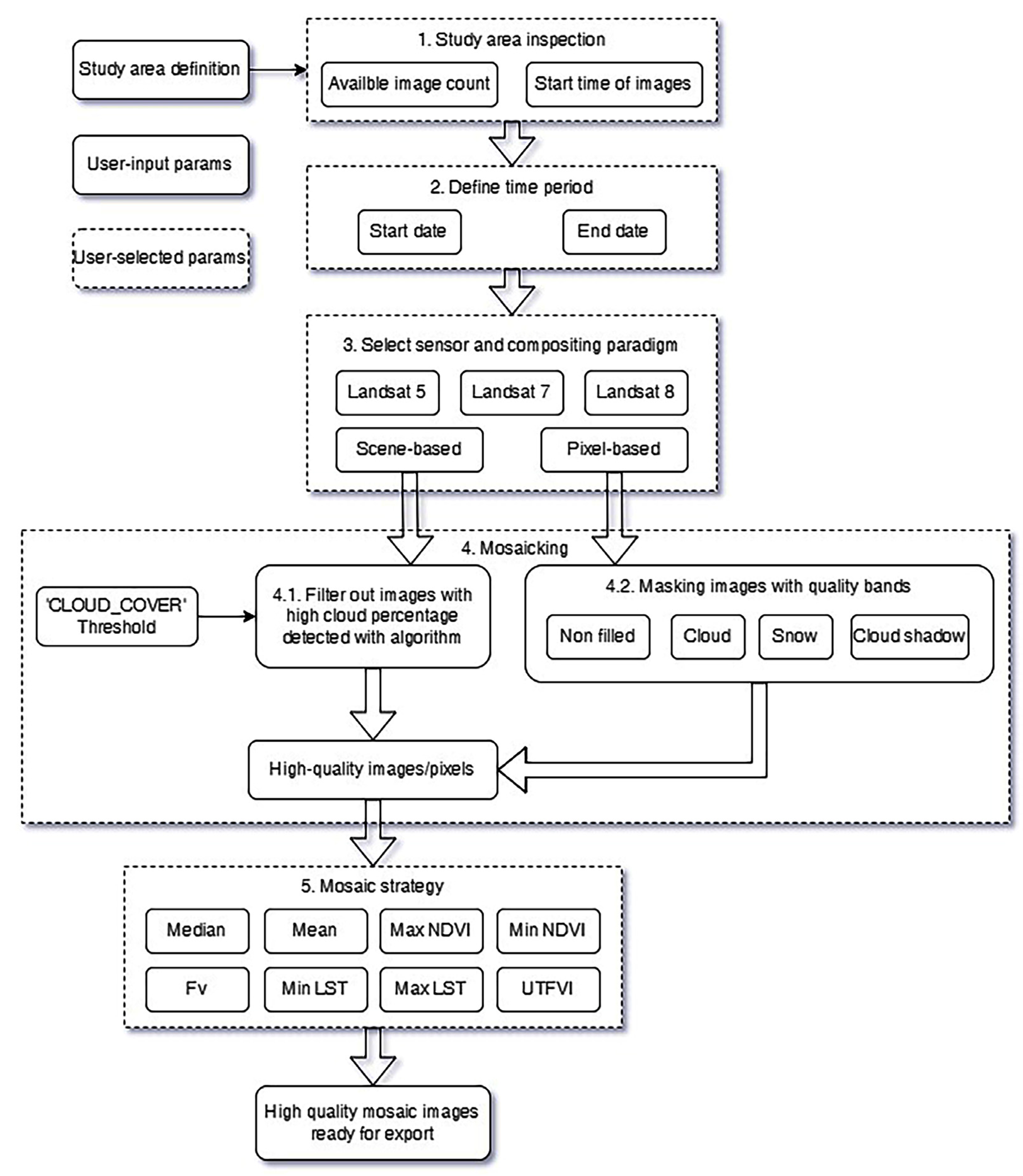
Figure 2 illustrates the high-quality Landsat mosaic image processing framework proposed in this article, with the assistance of the GEE platform. The steps are outlined as follows:
Step 1: Load the study area boundaries and verify the number of available images and that the starting times of those images are as specified by the user.
Step 2: Specify a period for mosaicking with user input for start and end dates.
Step 3: Select a composite model, which could be scene-based or pixel-based.
Step 4: Trim the images to the boundaries of the study area.
Step 5: Use algorithms to produce high-quality composited mosaic images and histograms.
In Step 4, when trimming the images to the boundaries of the study area and calculating the NDVI, SWVI, NBR, and UTFVI indices, the following corresponding formulas are applied:
The normalized difference vegetation index (NDVI) is a commonly used tool to determine the presence of live green vegetation in remote sensing data. The calculation applies the following formula:
N D V I = N I R R E D N I R + R E D
where RED is the reflection coefficient in the red spectral zone, corresponding to the Landsat TM band 3 (0.63–0.69 µm) and Landsat OLI band 4 (0.64–0.67 µm); NIR is the reflectance in the near-infrared zone that corresponds to the Landsat TM band 4 (0.76–0.90 µm) and Landsat OLI band 5 (0.85–0.88 µm);
The effectiveness of the short-wave vegetation index (SWVI) in monitoring the state of vegetation was explored, as this spectral index is sensitive to the moisture content in the vegetation cover. It is calculated using the following formula:
S W V I = N I R S W I R N I R + S W I R
where NIR is the reflection of vegetation cover in the near-infrared part of the spectrum with a range of band 4 (0.76–0.9 µm); SWIR is the reflection of vegetation cover in the mid-infrared part of the spectrum with a range of band 5 (1.55–1.75 µm).
The normalized burn ratio (NBR) is used to identify burned areas and assess the severity of the burn. It is calculated by conventionally taking the ratio of the near-infrared (NIR) and short-wave infrared (SWIR) values.
N B R = N I R S W I R N I R + S W I R
where NIR is the reflection of vegetation cover in the near-infrared part of the spectrum within the range of band 4 (0.76–0.9 µm); SWIR is the reflection of vegetation cover in the mid-infrared part of the spectrum with a range of band 7 (2.107–2.294 µm).
In urban regions, the UHI effect has a crucial impact on the environment and the well-being of urban dwellers. Various thermal comfort indices evaluate the UHI effect on urban life quality. This study utilized the urban thermal field variance index (UTFVI), calculated through Equation (4). The study used the urban thermal field variance index (UTFVI) to determine the location of UHIs in Moscow.
U T F V I = T s T m T s
where T s is the ground surface temperature, and T m is the average ground surface temperature in the research area.
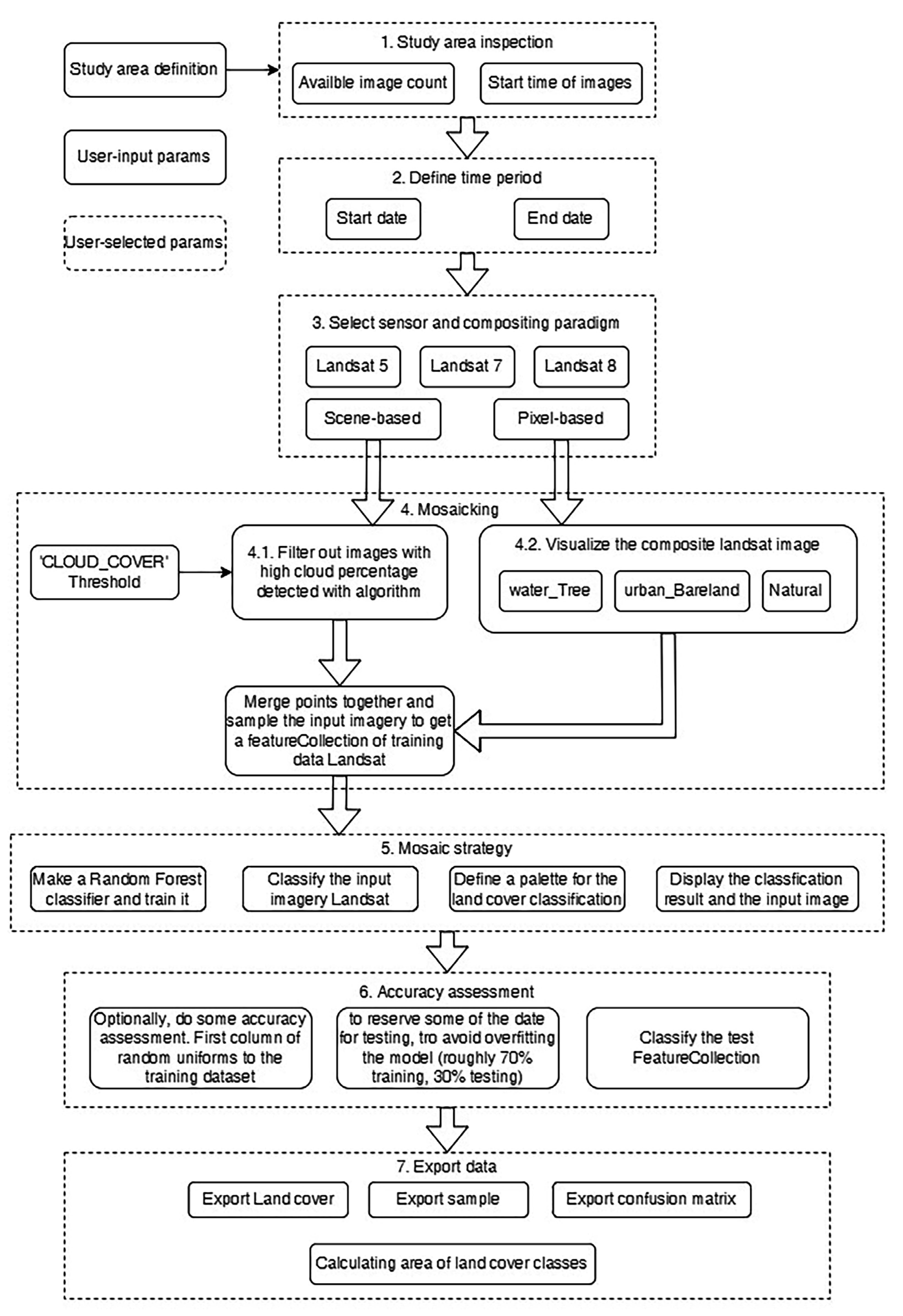
This study used the random forest algorithm based on the chosen period to determine the land cover classification. The algorithm, known as random forest (RF), was developed by Tin Kam Ho through the application of the random subspace technique (Laboratories et al., 1995) [21] and was later improved by Leo Breiman [22]. Random forest is a widely utilized machine learning technique that is categorized as supervised learning and can be utilized for classification and regression tasks. It relies on the idea of ensemble learning, which involves combining multiple classifiers to tackle complex problems and enhance the performance of the model [23]. The steps are illustrated in a workflow diagram (Figure 3).

3. Results

3.1. Analysis of the Landsat Spectral Index over the Years

This study set the start date to 1 January 1997 and the end date of the analysis to 1 January 2021. With the help of the cloud mask algorithm (cloud_mask_L457 and cloud_mask_L8), we removed pixels covered by clouds, which affect the accuracy of the results. The satellite images were filtered, provided that clouds covered no more than 20% of the study area.
The normalized difference vegetation index (NDVI), normalized burn ratio (NBR), and soil-adjusted vegetation index (SWVI) are commonly used to analyze plant growth trends and other soil surface changes.
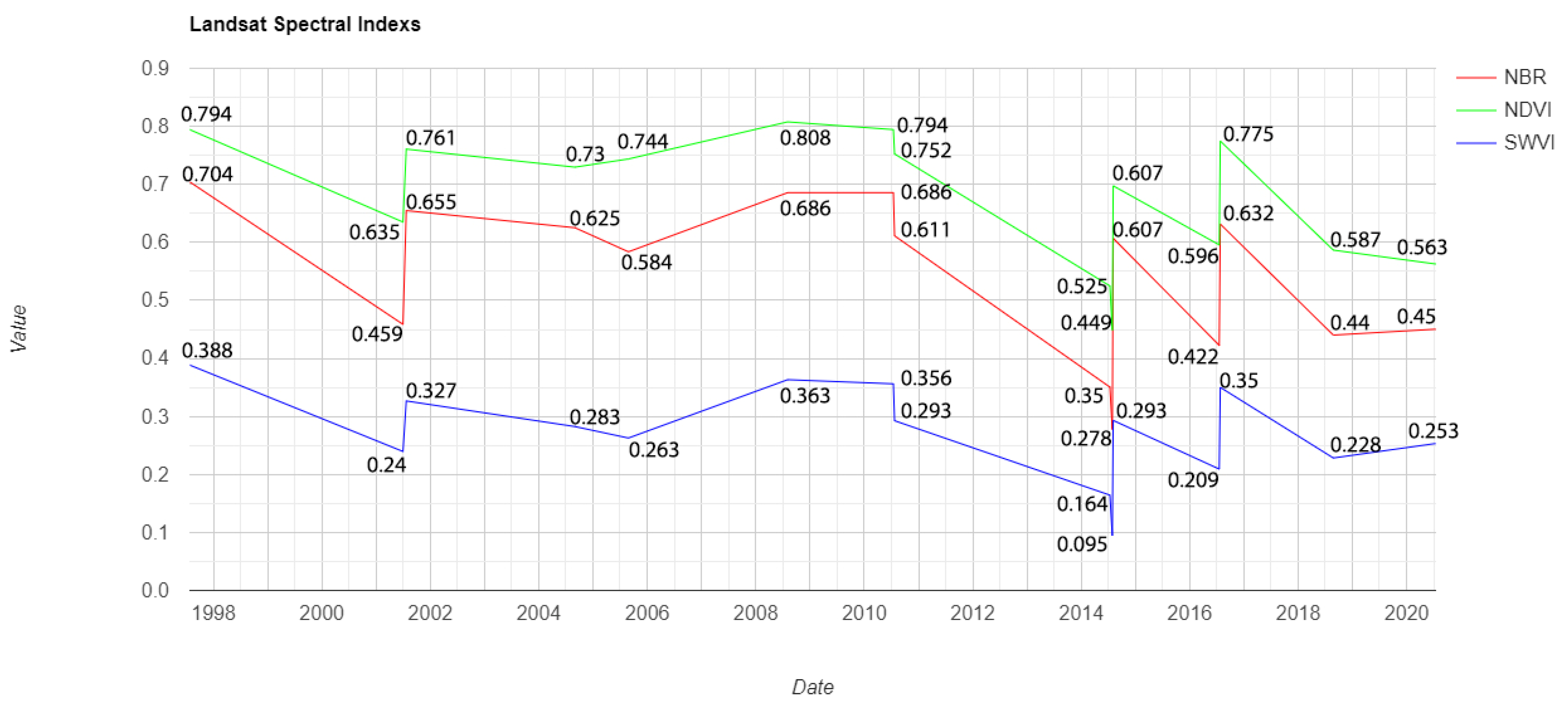
The NDVI, SWVI, and NBR from 1997 to 2021 were proportional to each other and tended to decrease. This shows that Moscow’s density of trees and green areas has been sharply declining. Within 24 years, the NDVI decreased 1.41 times or 30%. The SWVI for health monitoring and dead tree locations decreased 1.53 times, equivalent to 34.39%. For the NBR, showing the areas affected by forest fires, the reduction was 1.56 times, equivalent to 36%.
The NDVI measures the amount of green in an image. The NDVI ranges from −1 to 1, with values closer to 1 indicating denser green. Based on the parameters shown in Figure 4, the NDVI of Moscow gradually decreased from 0.794 (1997) to 0.563 (2021), showing a trend of vegetation decline.
The normalized burn ratio (NBR) is commonly used to quantify forest fire zones. This index is a ratio between the wildfire wavelengths and the vicinity’s average wavelengths. The NBR represents burnt areas with lower values than unburnt areas. In Figure 4, Moscow’s NBR index decreased from 0.704 (1997) to 0.45 (2021), indicating a tendency for forest fires and shrinking vegetation.
The soil-adjusted vegetation index (SWVI) measures the amount of vegetation along watercourses and open areas used for growing crops. The higher the SWVI, the denser the green. In Figure 4, Moscow’s SWVI decreased from 0.388 (in 1997) to 0.253 (in 2021), indicating a trend of vegetation reduction along watercourses and croplands.
The results of the above calculations are derived from the code lines depicted in the link below: https://code.earthengine.google.com/7edfebb6a1970b1795141ad50276b846 (accessed on 1 September 2022).

3.2. Classification of Land Cover by Machine Learning

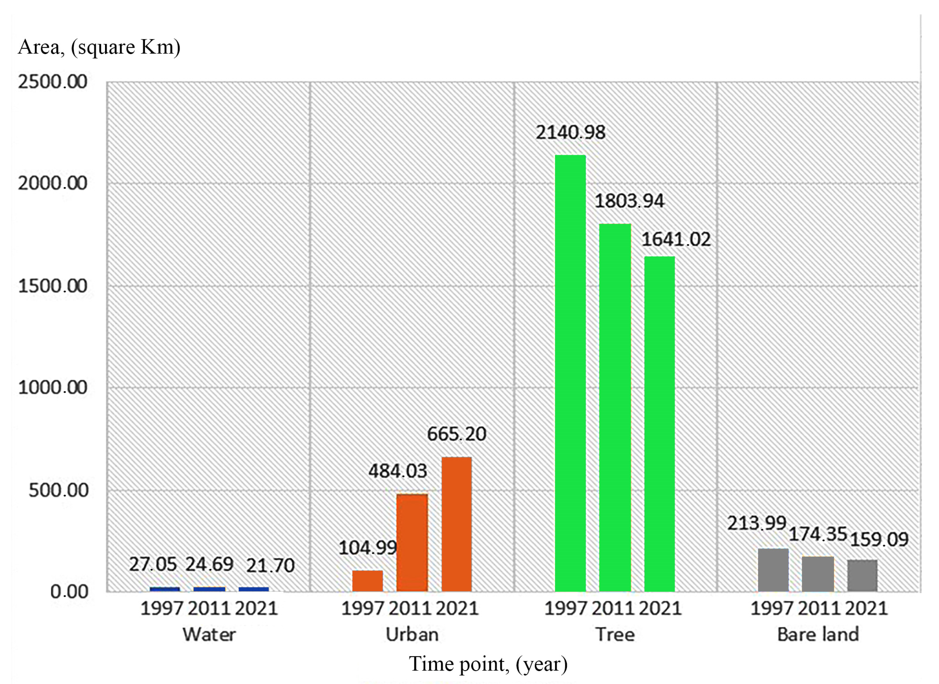
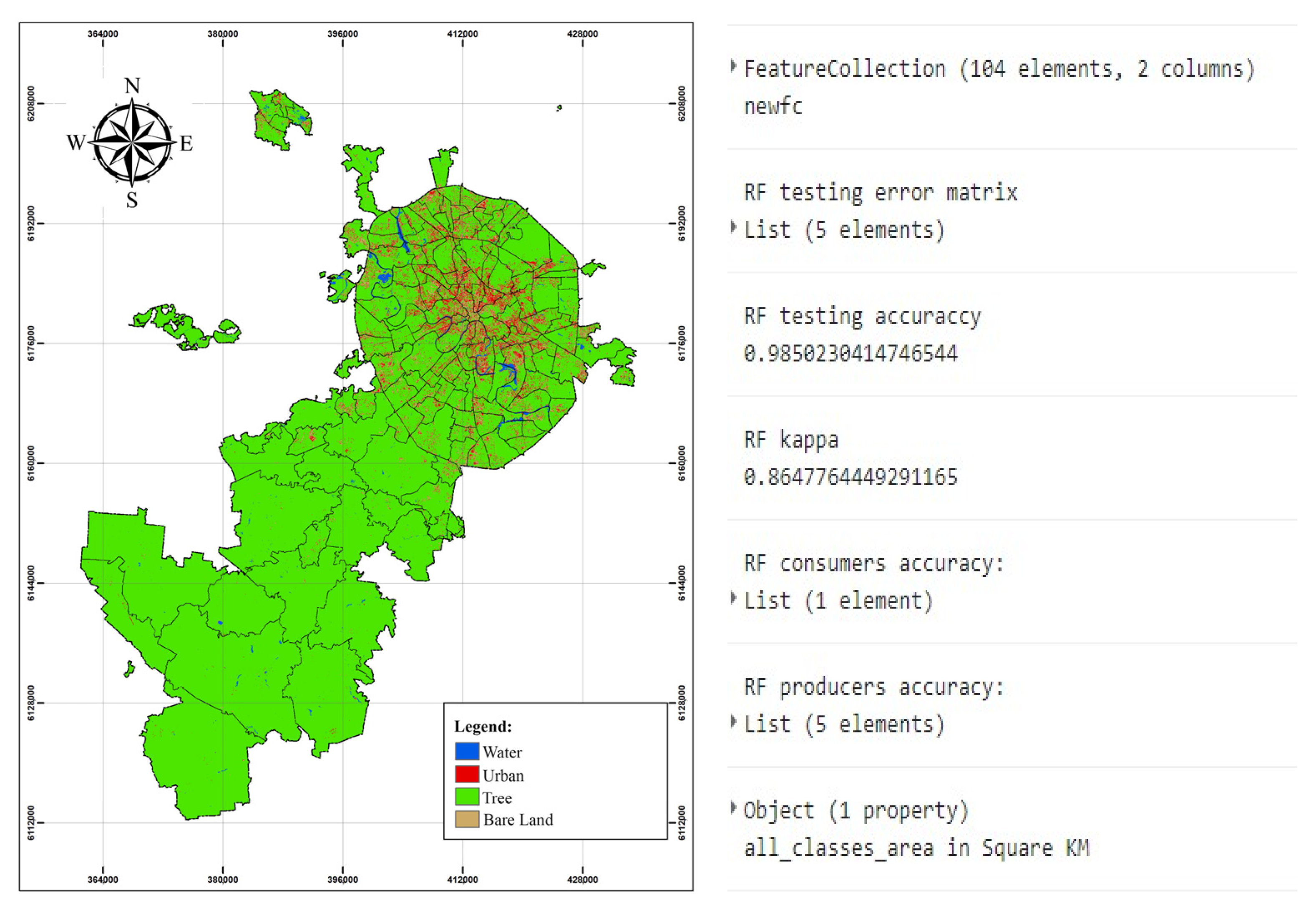
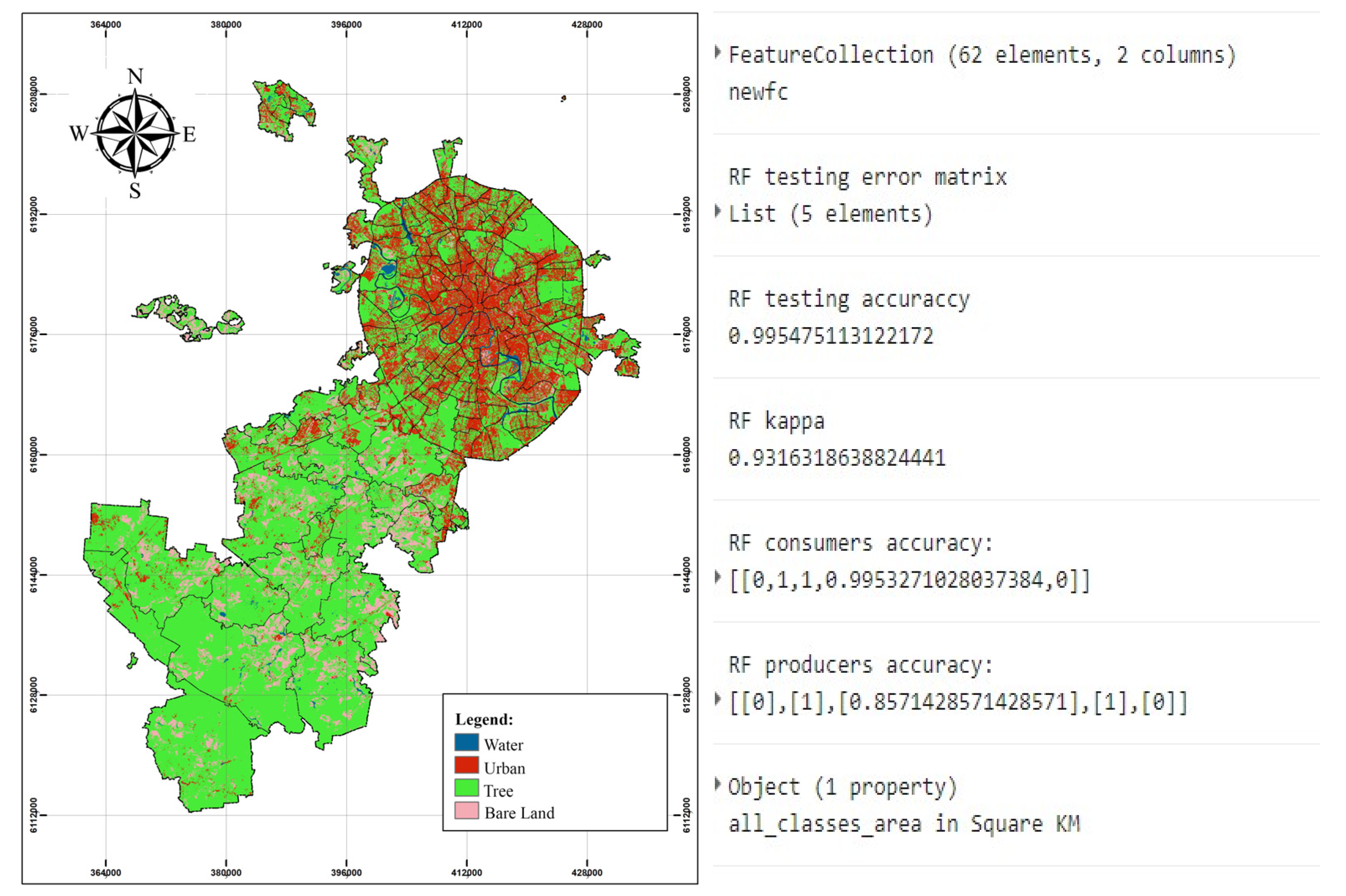
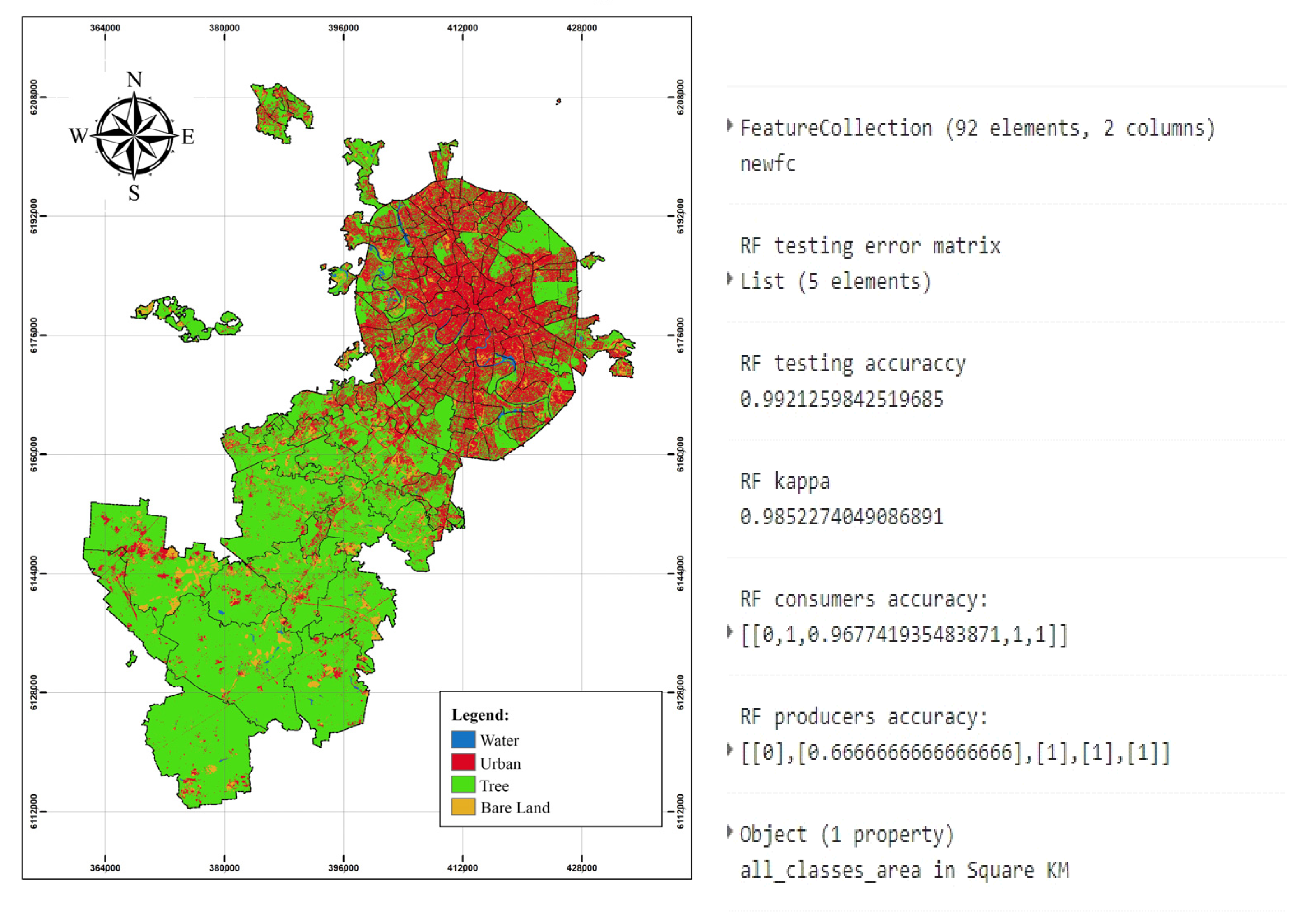
The Moscow landscape in terms of land use area has significantly changed from 1997 to 2021, with a notable decline in the extent of bare land and trees and a six-fold increase in the urban area (as shown in Table 2 and Figure 5).
The analysis of Moscow’s land cover was conducted over 24 years from 1997 to 2021, utilizing data from the Landsat 5, 7, and 8 satellites. The images provided by the satellite were cropped according to the Moscow boundary. The cloud mask was processed with the “cloud mask L457” algorithm for the Landsat 5 and 7 images and the “cloud mask L8” algorithm for the Landsat 8 images. Combining image channels produced composite images. The composite images of water and trees were combined from bands 2, 3, and 4. The composite images of urban and bare land were combined from bands 3, 4, and 5. The composite images of nature were combined from image channels 1, 2, and 3. Next, we created a training sample layer containing the following overlay types: water, urban, trees, and soil. Based on the previous training sample layer, we applied the random forest algorithm for machine learning and to enhance classification accuracy. The classification was achieved using 70% of the data for training and the remaining 30% for testing. Figure 6, Figure 7 and Figure 8 show the calculated results and images.
The urban area was primarily concentrated in the northern regions and gradually decreased toward the southwestern part of the city. Despite the rapid pace of urban expansion and development, more investment is needed in creating sufficient green spaces, resulting in a dearth of green vegetation in central Moscow and a reduction in green areas. This, in turn, has had a detrimental effect on the city’s ecology and has exacerbated the formation of UHIs and UPIs. The results of the above calculations were derived from the code lines depicted in the link below: https://code.earthengine.google.com/00edfa244cdd337c93d6071cb32d765d (Landsat 5); https://code.earthengine.google.com/74e29f322d11a56ad8aaf8d9d46e4862 (Landsat 7); https://code.earthengine.google.com/6a6997d54ac044de3a05b9913fac0515 (Landsat 8), all accessed on 1 September 2022.

3.3. Calculate Land Surface Temperature and Locate Surface Urban Heat Islands

3.3.1. Analysis of Moscow Surface Temperature by Time Series from 2015 to 2019

In a grid of 1200 × 1220 km, the MOD11A2 V6.1 product delivers an 8-day average land surface temperature (LST). The MOD11A2 pixels are a simple eight-day average of all the matching MOD11A1 LST pixels. Thus, this work uses MOD11A2.061 Terra Land Surface Temperature and Emissivity 8-Day Global 1 km to examine the surface temperature of Moscow from 2015 to 2019.
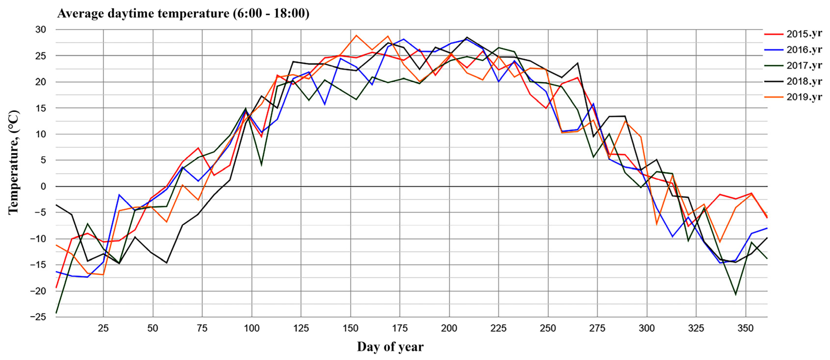
Moscow’s daytime LST and nighttime LST are shown in Figure 9 and Figure 10. The analysis results of Moscow’s mean daytime surface temperatures (Figure 9) show:
On the 185th day of 2015, the highest average daytime temperature reached 26.18 °C;
On the 177th day of 2016, the highest average daytime temperature reached 28.18 °C;
On the 225th day of 2017, the highest average daytime temperature reached 26.54 °C;
On the 209th day of 2018, the highest average daytime temperature reached 28.55 °C;
On the 153rd day of 2019, the highest average daytime temperature reached 28.89 °C.
The highest average nighttime temperature in 2019 was higher than the average maximum daytime temperature in 2015, about 2.71 °C.
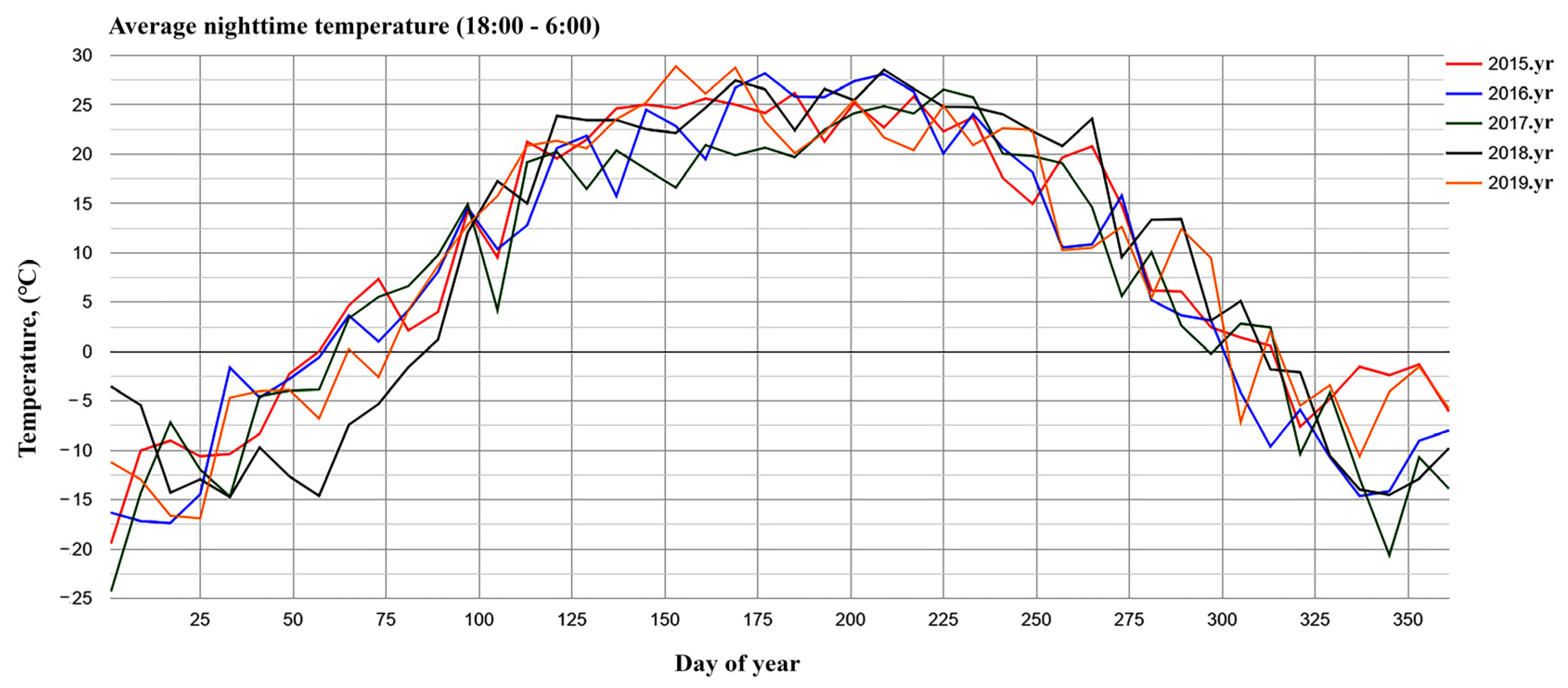
The analysis of the results of Moscow’s mean night-time surface temperatures (Figure 10) showed:
On the 217th day of 2015, the highest average night-time temperature reached 17.06 °C;
On the 177th day of 2016, the highest average night-time temperature reached 20.05 °C;
On the 209th day of 2017, the highest average night-time temperature reached 17.43 °C;
On the 209th day of 2018, the highest average night-time temperature reached 17.91 °C;
On the 169th day of 2019, the highest average night-time temperature reached 18.52 °C;
The highest average night-time temperature in 2019 was above the maximum in 2015, about 1.46 °C.
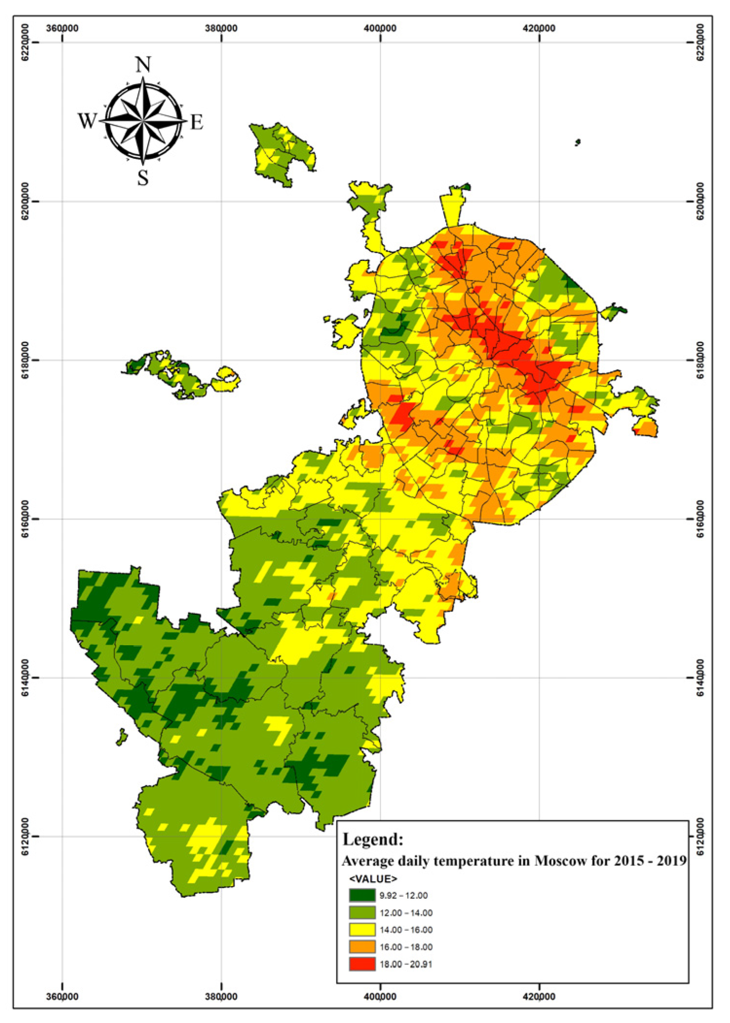
Over the past decade in Moscow, there has been a pronounced shift in land cover due to intense urbanization. This shift has also impacted the LST of the city. Figure 11 depicts the average temperature over the last five years in Moscow, with the central regions recording an average temperature of 18–20.91 °C, while the suburbs and rural areas had an average temperature of 9.92–12 °C, leading to a temperature difference of about 8.08 to 8.91 °C. This temperature disparity indicates the negative impact of the SUHI effect in Moscow. Although urbanization cannot be halted, it can be managed by creating conditions enabling autonomous and sustainable development. It is essential to identify the most valuable natural areas, define their boundaries, and regulate the exchange of substances, energy, and information between them. This will necessitate a more complex relationship between the anthropogenic and natural environments and the development of appropriate mechanisms to ensure a balanced interaction.
According to Shukurov et al. (2020) [24], the SUHI is defined as a phenomenon where the atmospheric layer experiences a difference in daytime and night-time temperatures of approximately 7–12°, as reflected in the statistics in Table 3. This study found evidence of a SUHI effect in Moscow.
The results of the above calculations were derived from the code lines obtained from the following link: https://code.earthengine.google.com/66dde090f75f43e8667a4318563d9bbe (accessed on 1 September 2022).

3.3.2. Determining the Location of SUHIs in the Moscow Area

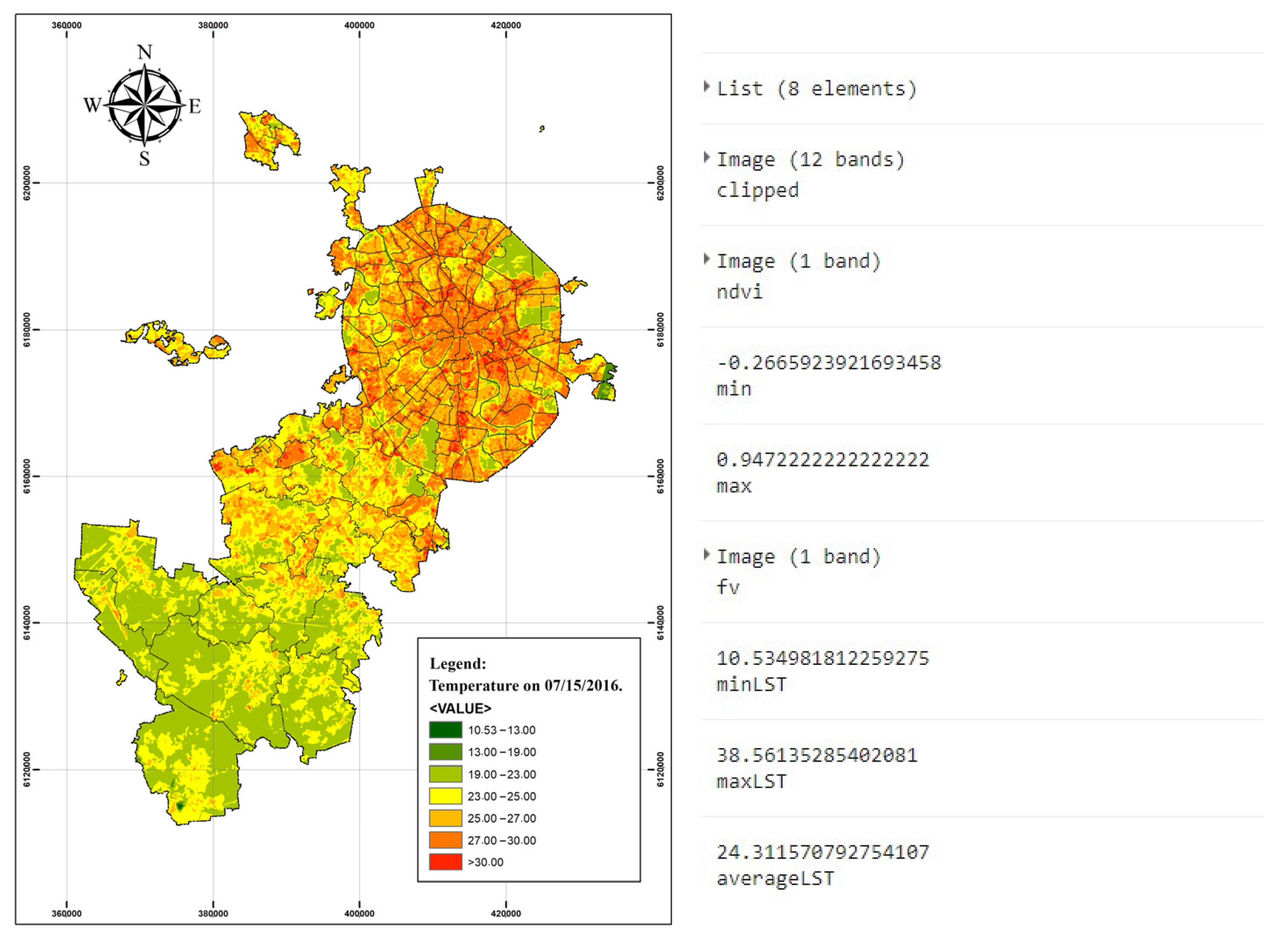
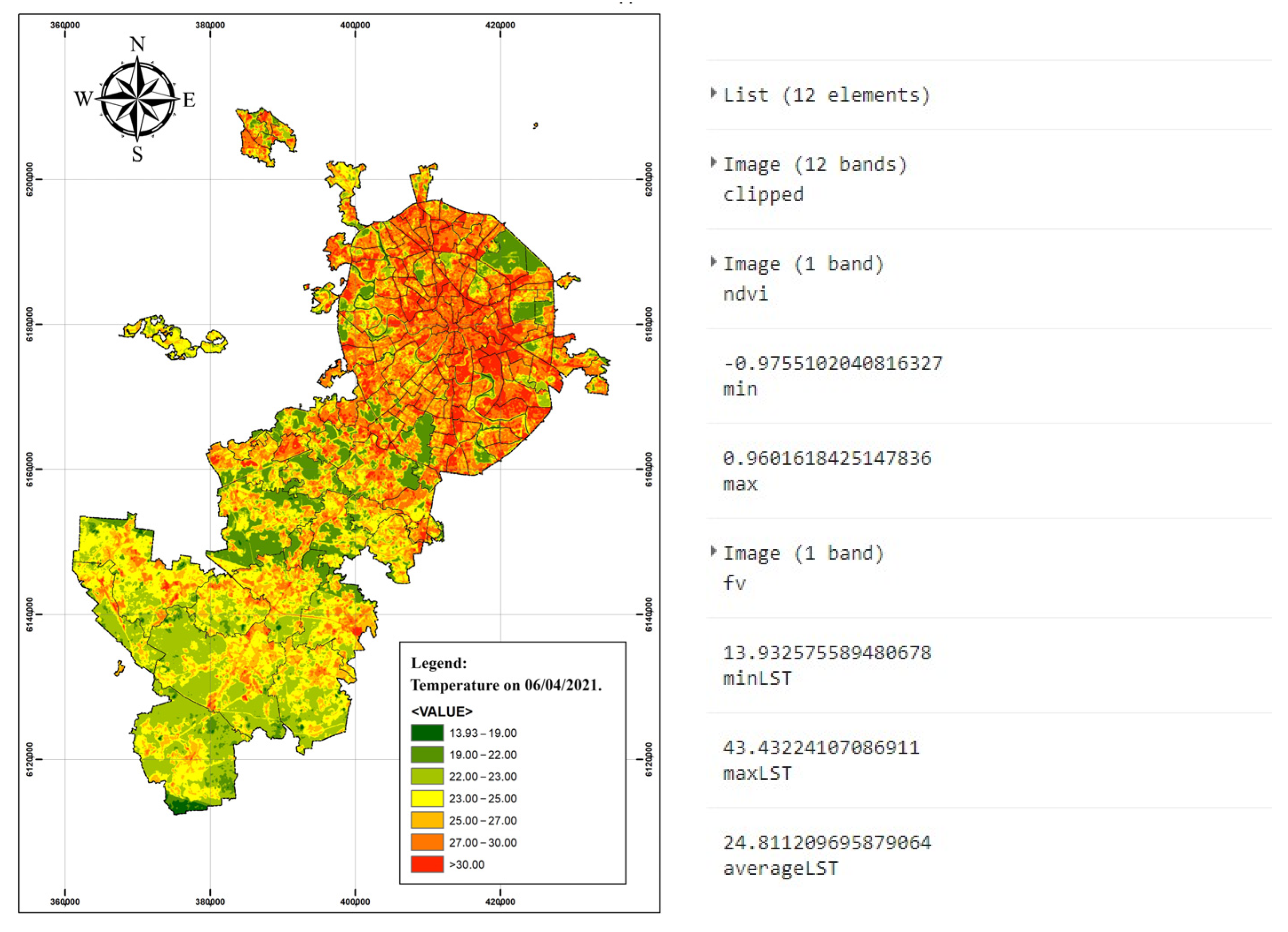
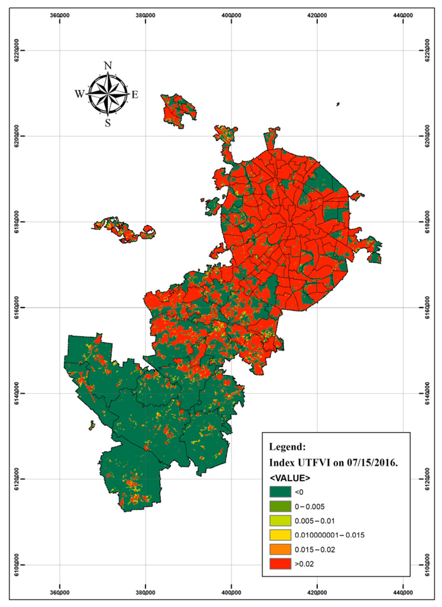
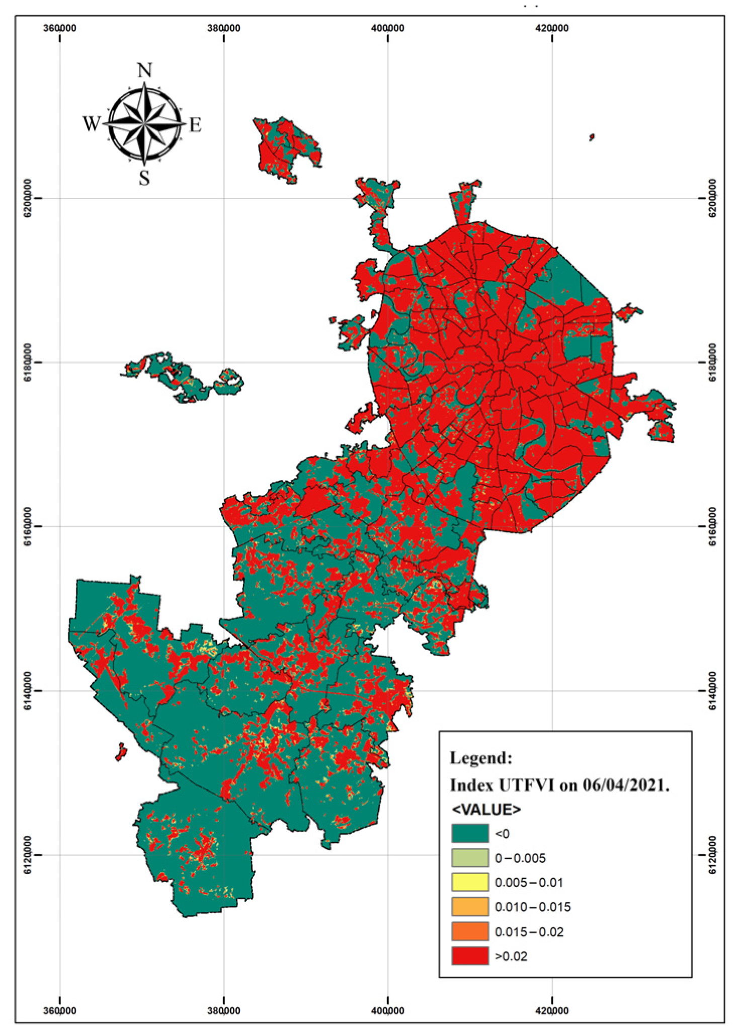
We extended our findings through a comprehensive evaluation of LST in the hot seasons of 2016 and 2021. The data were collected from the Landsat 8 satellite, operated by the USGS Landsat 8 Surface Reflectance Tier 1, using remote sensing techniques. The images were analyzed for 2016 and 2021 after applying cloud coverage filters and a masking algorithm (MaskL8sr) to ensure less than 10% cloud interference. The land surface temperature was analyzed using satellite images taken on 15 July 2016 and 4 June 2021. The temperature was calculated using the NDVI and band 10 image data, with the conversion indices shown in Figure 12 and Figure 13. Additionally, simulation images for surface temperature are presented in these figures.
The urban thermal field variance index (UTFVI) is used to evaluate the ecological state of urban environments. It is widely used because it directly relates to LST and considers the thermal impact of different subareas within an urban agglomeration. The UTFVI provides a comprehensive view of the thermal variance across different geographic subareas, making it an effective tool for assessing the impact of urbanization on the environment.
The urban thermal field variance index (UTFVI) values were categorized into six groups corresponding to an environmental assessment interpretation. Table 4 presents the threshold values for each urban area’s thermal field dispersion index categories, from no SUHI (excellent) if LSTurban-pixel < LSTurban-mean to strongest (worst) with UFTVI > 0.02, a situation that occurs when the value of LSTurban-pixel is several degrees higher than LSTurban-mean.
The calculation of the UTFVI using the city’s surface temperature showed that in the central areas of the city, the intensity of the heat islands exceeded the threshold assessed in Table 3 (Figure 14 and Figure 15). In these areas, people were subjected to heat stress. The results of the above calculations were derived from the code lines depicted in the following link: https://code.earthengine.google.com/e06787111994baee6d741716f118018a (accessed on 1 September 2022).

4. Discussion

4.1. Assessing the Influence of SUHIs on UPI

The surface urban heat island (SUHI) effect can exacerbate air pollution in urban areas. This phenomenon arises when the temperature in an urban location surpasses that of adjacent rural areas due to the absorption and reradiation of heat by materials such as concrete and asphalt as well as human activities such as energy usage and transportation [26]. The higher temperatures in urban areas can create local wind patterns that trap atmospheric pollutants, such as vehicle emissions and industrial pollution. This can lead to higher concentrations of air pollutants, negatively affecting urban residents, particularly vulnerable populations such as children, the elderly, and those with respiratory or cardiovascular conditions.
Fine particles, particularly PM2.5, in the atmosphere can directly decrease solar radiation and reduce surface temperature by up to 1 K [27]. However, the extent of this temperature decrease depends on the chemical composition of the particles. Sulfate aerosols, which scatter light but do not absorb it, lead to a decrease in surface temperature when their concentrations increase [28]. Conversely, while black carbon is the primary component of the atmospheric aerosols that absorb radiation, it can also diminish the cooling impact of aerosols by heating the atmosphere near the top of the boundary layer [29].
Moreover, the regional characteristics of aerosol properties also play a significant role in determining the radiation forcing and surface temperature. Different regions may have inherently different PM2.5 loads and compositions, resulting in different radiation forcing and temperature effects. A case in point is a study on aerosol particles conducted in Nanjing, which revealed that the particles present in urban centers had a high absorption capacity. In contrast, those present in suburban areas showed scattering solid traits. This discrepancy resulted in dissimilar radiation forcing and temperature effects in the respective regions [30]. Overall, the impact of particulate matter on surface temperature is complex and depends on various factors, including the aerosol particles’ chemical composition and regional characteristics.
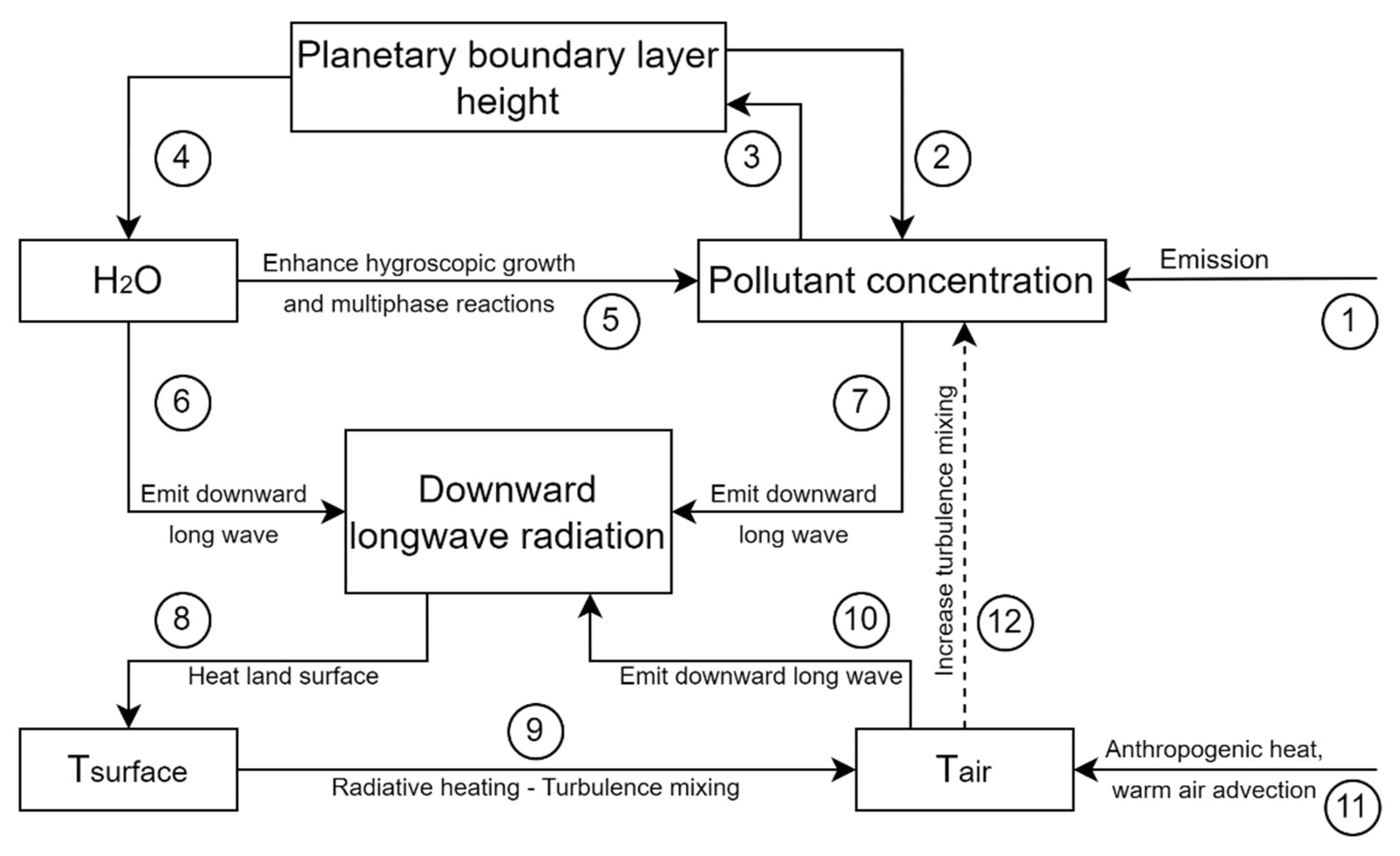
Figure 16 illustrates the inter-related processes and feedback between pollutant concentration, planetary boundary layer height, water vapor, downward longwave radiation (DLR), and temperature, as outlined by Petäjä et al., 2016 [31]. The processes described in Steps 1 to 3 produce a positive feedback mechanism, according to both Tie et al., 2017 [32] and Liu et al., 2018 [33]. Ref. [34] supports that UPI negatively correlates with SUHI, primarily through Steps 1, 7, 8, 9, and 12 [35]. Process 6, as demonstrated by Yamada et al., 2012 [36], reveals how water vapor becomes one of the primary drivers of DLR. Meanwhile, Cao et al., 2016 [37] and Li et al., 2018 [34] suggested that air pollution contributes to downward longwave radiation for Step 7.
The significance of investigating the effects of the combination of SUHIs and UPIs has been highlighted since 2004 [38]. With the widespread use of remote sensing in climatology, further research has revealed other factors that interact with urban heat islands, including water vapor. In a study conducted in Shanghai [39], the correlation between heat islands and pollution was established by combining satellite data on the Earth’s surface temperature, albedo, water vapor, cloud cover, and land cover with continuous observations of aerosol optical thickness on Earth to track daily, seasonal, and interannual changes. The monthly aerosol optical thickness was higher in Shanghai than in rural areas, with the most significant changes occurring after rain and during periods of intense movement. There were significant differences in cloudiness and water vapor between urban and rural areas.
In a recent publication in Nature Communications (Cao et al., 2016) [40], evidence was presented to support the hypothesis that pollution from urban haze has a biogeochemical effect that contributes to the formation of urban heat islands. The authors used satellite observations (MODIS) from 2003 to 2013 and climate model calculations to quantify the contribution of urban heat islands in 39 Chinese cities at night. In semiarid urban areas, the urban heat island effect increased by 0.70 ± 0.26 °C. However, the study showed that wet and semiwet climates were less sensitive to the longwave radiation impact of coarse aerosols, consistent with the findings of Jonsson et al. (2004) [41]. The study revealed high mean ground-level urban heat island values at night and weak urban heat island values during the day, regardless of the average annual amount of precipitation (Zhou et al., 2014) [42]. Night-time spatial variations were primarily correlated with the difference in aerosol optical thickness between urban and adjacent rural areas, indicating that denser haze preceded more substantial urban heat islands. However, this correlation disappeared during the day. Based on their findings, the authors concluded that fog pollution was the cause of accelerated warming observed in China (double the global average increase in night-time temperature over the past decade). Li et al., 2018 [34] used a similar approach, using multiyear satellite observations of land surface temperature (LST) and aerosol optical thickness, as well as measurements of particulate matter (PM10), air temperature, incoming radiation, cloud cover, and wind speed at twelve stations to identify the potential interaction between urban heat islands and urban pollution indices [34]. LST and air temperature were indirect indicators of surface and atmospheric urban heat islands, whereas PM10 and aerosol optical thickness were indirect indicators of near-surface and atmospheric pollution.
Our recent research paper, published in Ecological Informatics in 2022, looks closely at the relationship between SUHI and UPI [43].
Assessing the connection between SUHIs and UPIs demands expertise and substantial resources. According to traditional research methods, it will take a long time to evaluate the process through which the surface temperature of the city changes with the change in particulate matter concentration. The cloud computing platform is an excellent upgrade for big data retrieval to assess and analyze the process of surface urban heat island formation. In this article, we presented the results of the evaluation of SUHI formation in Moscow and compared them with the results of the UPI formation shown in the previous article.
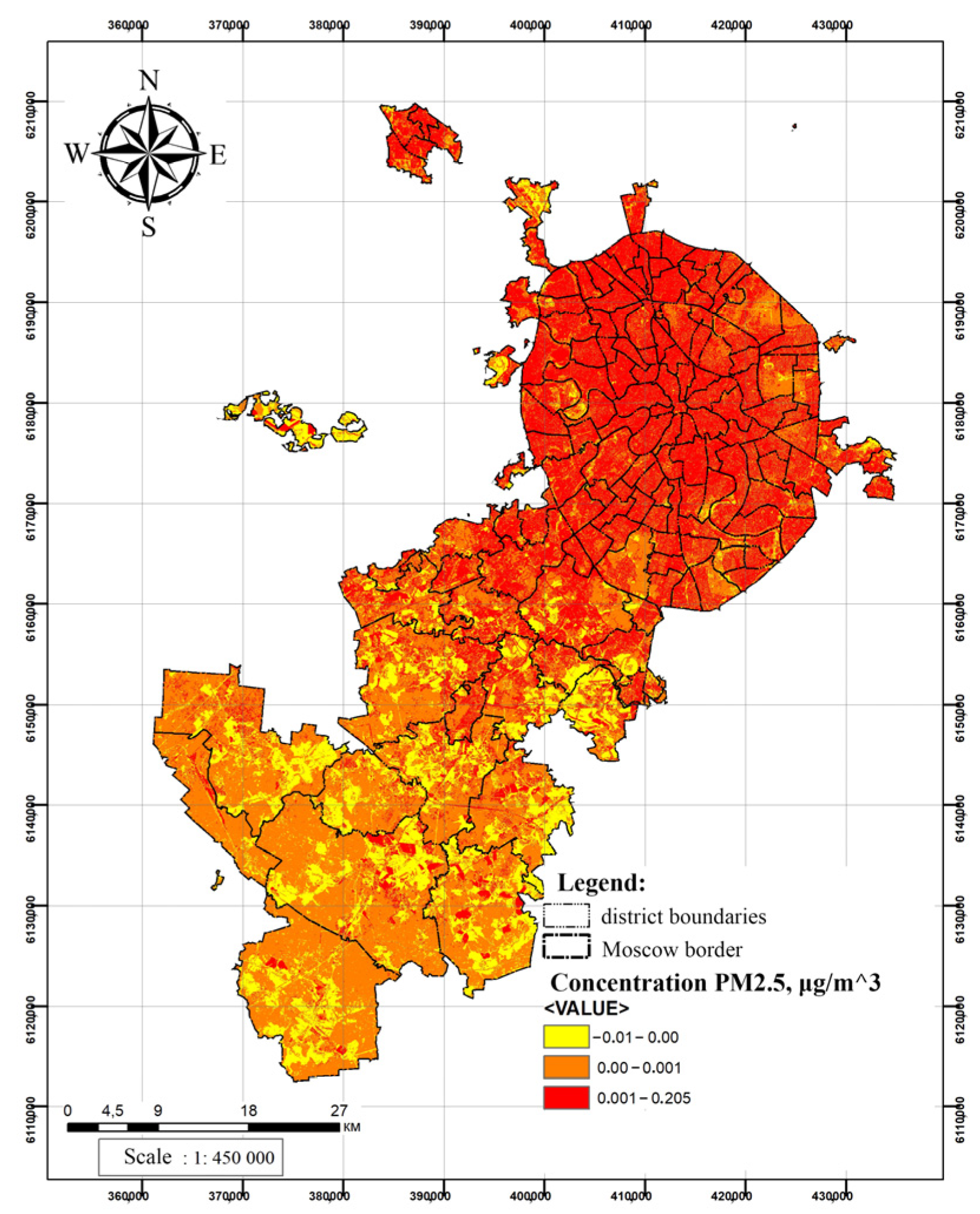
Our assessment results revealed that in the central district of Moscow, which the SUHI significantly impacts, UPIs also emerged in the exact locations as the SUHIs (as depicted in Figure 17 and Figure 18). The visualization of the UTFVI in urban areas within Moscow’s boundaries also displays the location of the SUHIs.

4.2. Future Research

Google Earth Engine (GEE) has gained popularity in environmental and urban studies due to its cloud-based geospatial processing power and vast collections of geospatial datasets such as Landsat and MODIS. Despite its potential, ecological and urban modelers face three significant challenges when using GEE. First, current GEE applications remain confined to basic mapping and underutilize its complete capabilities. Second, modelers must overcome technical complexities to effectively develop image-processing-based environmental models. Lastly, many ecological and urban modelers remain unaware of GEE’s unprecedented geospatial processing capacity and extensive collection of big geospatial datasets, resulting in unexplored potential. Thus, the potential of GEE to support ecological and urban modeling remains largely untapped. In future studies, we aim to improve GEE’s functions with custom and functional sets to model sustainable urban growth under the influence of SUHIs and UPIs.
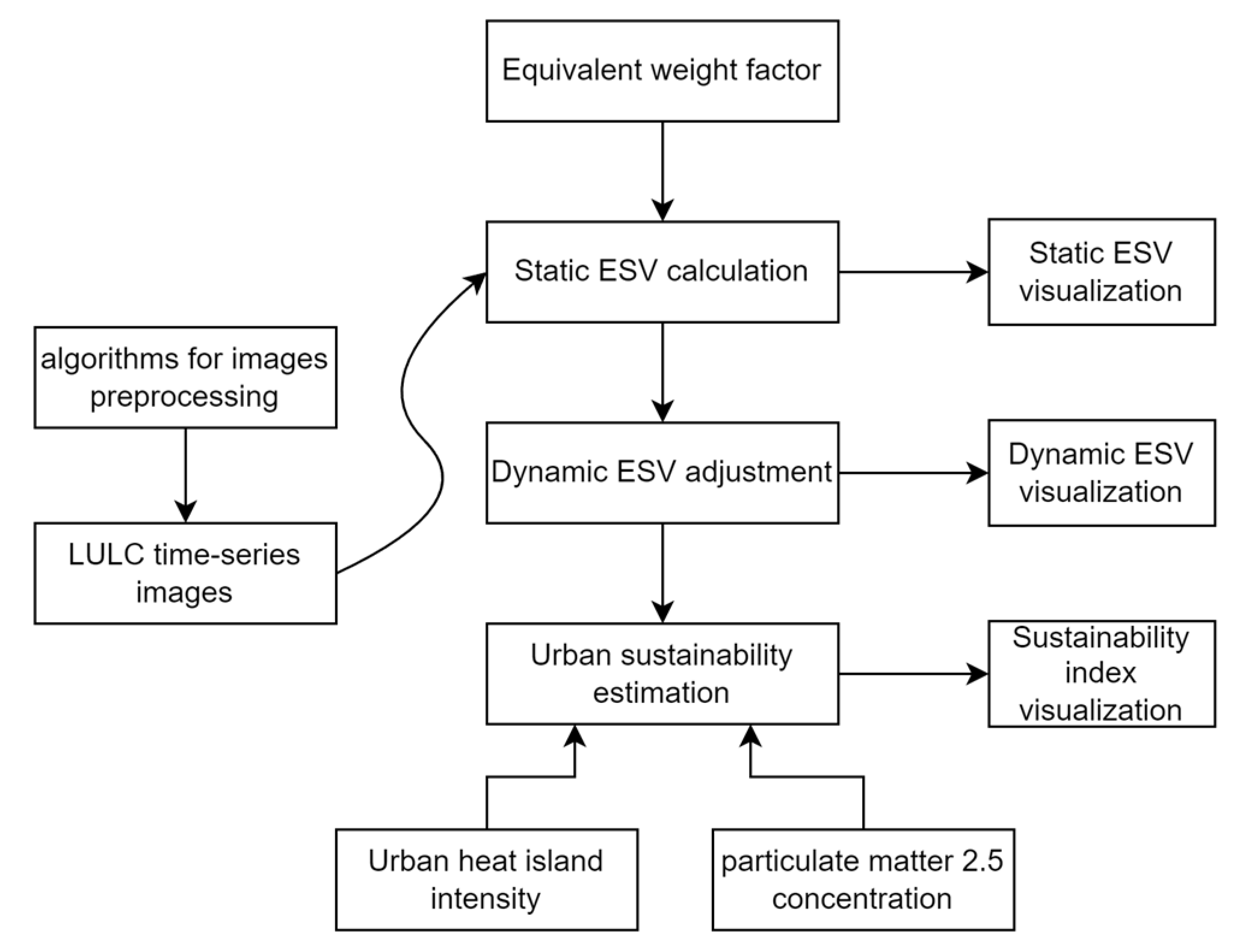
The logical flow of cloud-based sustainable urban modeling processes is displayed in Figure 19. Image retrieval and preprocessing are vital to derive a collection of land-use cover over a specified time frame, involving data normalization and time series image overlay. Algorithms such as random forest (RF), calculation, and training and testing samples are utilized to increase land use cover classification accuracy. In the context of ecosystem service value (ESV), urban sustainability modeling entails determining the weight parameters of land use categories and ecological functions, computing static ESV, computing dynamic ESV by integrating social development variables, and modeling urban sustainability while considering gross domestic product (GDP) and per capita net income (PCNI). Finally, the modeling outcomes are visualized and analyzed.

5. Conclusions

Moscow was chosen as the research subject due to its characteristics and problems as a megacity. Previous studies on identifying polluted areas were conducted using ArcGIS software, conversion of Landsat satellite images, data collected at monitoring stations as part of the “City Air” project in Moscow, and other spatial analysis tools. This article presents further research conducted to identify surface urban heat islands in Moscow and assess the interaction between SUHIs and UPIs using the Google Earth Engine (GEE) geospatial analysis platform. Using numerical modeling of the UTFVI, the locations of the surface urban heat islands in Moscow were identified.
Empirically, it was established that, based on the analysis of the obtained images, the areas of concentrated air pollution and high land surface temperature were mainly concentrated in the northern and central areas of the city, with a decrease in adverse factors to the southwest. The results of the analysis of the changes in the vegetation cover in Moscow from 2015 to 2019, conducted using cloud computing and machine learning, showed that rapid urbanization directly affects the thermal comfort of its inhabitants. This rapid urban growth creates ecological imbalances and harms the natural environment, thus creating conditions for the progression and transformation of SUHI and UPI.
The study introduced a novel method of utilizing cloud computing to gather geospatial data for analyzing the relationship between UPIs and SUHIs. Machine learning tools can customize and modify the data. However, GEE’s potential in ecological modeling remains largely unexplored. Future studies aim to leverage custom functional sets to enhance GEE’s capabilities for modeling sustainable urban growth under the influence of SUHIs and UPIs.

Author Contributions

M.T.L.: writing—original draft, data curation, methodology, conceptualization, formal analysis. N.B.: methodology, writing—review and editing, supervision. All authors have read and agreed to the published version of the manuscript.

Funding

The authors gratefully acknowledge financial support from the Moscow State University of Civil Engineering and the Ministry of Education of Vietnam. The study was part of a science and technology project at the Ministry of Education of Vietnam from 2022 to 2023, B2022-MDA-12, according to Decision No. 2190/QD-BGĐT dated 30 June 2021.

Data Availability Statement

The data from the study are available on request.

Acknowledgments

We thank Nina Umnyakova from the Research Institute of Building Physics and Enclosing Structures of the Academy of Civil Engineering and Architecture (NIISF RAASN) for her advice.

Conflicts of Interest

The authors declare no conflict of interest.

References

  1. Wulder, M.A.; White, J.C.; Loveland, T.R.; Woodcock, C.E.; Belward, A.S.; Cohen, W.B.; Fosnight, E.A.; Shaw, J.; Masek, J.G.; Roy, D.P. The global Landsat archive: Status, consolidation, and direction. Remote Sens. Environ. 2016, 185, 271–283. [Google Scholar] [CrossRef] [Green Version]
  2. Roy, D.P.; Ju, J.; Kline, K.; Scaramuzza, P.L.; Kovalskyy, V.; Hansen, M.; Loveland, T.R.; Vermote, E.; Zhang, C. Web-enabled Landsat Data (WELD): Landsat ETM+ composited mosaics of the conterminous United States. Remote Sens. Environ. 2010, 114, 35–49. [Google Scholar] [CrossRef]
  3. Baer, Y.; Schneider, W.-D. Chapter 62 High-energy spectorscopy of lanthanide materials—An overview. In Handbook on the Physics and Chemistry of Rare Earths; Elsevier: Amsterdam, The Netherlands, 1987; Volume 10, pp. 1–73. [Google Scholar] [CrossRef]
  4. Loveland, T.R.; Dwyer, J.L. Landsat: Building a strong future. Remote Sens. Environ. 2012, 122, 22–29. [Google Scholar] [CrossRef]
  5. Whitman, R.T.; Park, M.B.; Ambrose, S.M.; Hoel, E.G. Spatial indexing and analytics on Hadoop. In Proceedings of the ACM International Symposium on Advances in Geographic Information Systems, Dallas, TX, USA, 4 November 2014; Volume 04-07-Nove, pp. 73–82. [Google Scholar] [CrossRef]
  6. Yu, J.; Wu, J.; Sarwat, M. GeoSpark: A cluster computing framework for processing large-scale spatial data. In Proceedings of the ACM International Symposium on Advances in Geographic Information Systems, Washington, DC, USA, 3–6 November 2015; Volume 03-06-Nove. [Google Scholar] [CrossRef]
  7. Hughes, J.N.; Annex, A.; Eichelberger, C.N.; Fox, A.; Hulbert, A.; Ronquest, M. GeoMesa: A distributed architecture for spatio-temporal fusion. In Proceedings of the Geospatial Informatics, Fusion, and Motion Video Analytics V, Baltimore, MD, USA, 20–21 April 2015; Volume 9473, p. 94730F. [Google Scholar] [CrossRef]
  8. Wijedasa, L.S.; Sloan, S.; Michelakis, D.G.; Clements, G.R. Overcoming limitations with landsat imagery for mapping of peat swamp forests in sundaland. Remote Sens. 2012, 4, 2595–2618. [Google Scholar] [CrossRef] [Green Version]
  9. She, X.; Zhang, L.; Cen, Y.; Wu, T.; Huang, C.; Baig, M.H.A. Comparison of the continuity of vegetation indices derived from Landsat 8 OLI and Landsat 7 ETM+ data among different vegetation types. Remote Sens. 2015, 7, 13485–13506. [Google Scholar] [CrossRef] [Green Version]
  10. Ferdman, M.; Adileh, A.; Kocberber, O.; Volos, S.; Alisafaee, M.; Jevdjic, D.; Kaynak, C.; Popescu, A.D.; Ailamaki, A.; Falsafi, B. Clearing the clouds. ACM SIGPLAN Not. 2012, 47, 37–48. [Google Scholar] [CrossRef]
  11. Gorelick, N.; Hancher, M.; Dixon, M.; Ilyushchenko, S.; Thau, D.; Moore, R. Google Earth Engine: Planetary-scale geospatial analysis for everyone. Remote Sens. Environ. 2017, 202, 18–27. [Google Scholar] [CrossRef]
  12. Lu, D.; Weng, Q. A survey of image classification methods and techniques for improving classification performance. Int. J. Remote Sens. 2007, 28, 823–870. [Google Scholar] [CrossRef]
  13. Gómez, C.; White, J.C.; Wulder, M.A. Optical remotely sensed time series data for land cover classification: A review. ISPRS J. Photogramm. Remote Sens. 2016, 116, 55–72. [Google Scholar] [CrossRef] [Green Version]
  14. He, J.; Harris, J.R.; Sawada, M.; Behnia, P. A comparison of classification algorithms using Landsat-7 and Landsat-8 data for mapping lithology in Canada’s Arctic. Int. J. Remote Sens. 2015, 36, 2252–2276. [Google Scholar] [CrossRef]
  15. Faridatul, M.I.; Wu, B. Automatic classification of major urban land covers based on novel spectral indices. ISPRS Int. J. Geo-Inf. 2018, 7, 453. [Google Scholar] [CrossRef] [Green Version]
  16. Chang, F.; Dean, J.; Ghemawat, S.; Hsieh, W.C.; Wallach, D.A.; Burrows, M.; Chandra, T.; Fikes, A.; Gruber, R.E. BigTable: A distributed storage system for structured data. In Proceedings of the OSDI 2006-7th USENIX Symposium on Operating Systems Design and Implementation, Seattle WA, USA, 6–8 November 2006; pp. 205–218. [Google Scholar]
  17. Corbett, J.C.; Dean, J.; Epstein, M.; Fikes, A.; Frost, C.; Furman, J.J.; Ghemawat, S.; Gubarev, A.; Heiser, C.; Hochschild, P.; et al. Spanner: Google’s Globally Distributed Database. ACM Trans. Comput. Syst. 2013, 31, 1–22. [Google Scholar] [CrossRef] [Green Version]
  18. Verma, A.; Pedrosa, L.; Korupolu, M.; Oppenheimer, D.; Tune, E.; Wilkes, J. Large-scale cluster management at Google with Borg. In Proceedings of the 10th European Conference on Computer Systems, EuroSys, Bordeaux France, 21–24 April 2015; Volume 2015. [Google Scholar] [CrossRef] [Green Version]
  19. Chambers, C.; Raniwala, A.; Perry, F.; Adams, S.; Henry, R.R.; Bradshaw, R.; Weizenbaum, N. FlumeJava. ACM SIGPLAN Not. 2010, 45, 363–375. [Google Scholar] [CrossRef]
  20. Gonzalez, H.; Halevy, A.Y.; Jensen, C.S.; Langen, A.; Madhavan, J.; Shapley, R.; Shen, W.; Goldberg-Kidon, J. Google fusion tables: Web-centered data management and collaboration. In Proceedings of the ACM SIGMOD International Conference on Management of Data, Indianapolis, IN, USA, 6–10 June 2010; pp. 1061–1066. [Google Scholar] [CrossRef]
  21. Ho, T.K. Random Decision Forests. In Proceedings of the 3rd International Conference on Document Analysis and Recognition, Montreal, QC, Canada, 14–16 August 1995. [Google Scholar]
  22. Deng, W.; Huang, Z.; Zhang, J.; Xu, J. A Data Mining Based System for Transaction Fraud Detection. In Proceedings of the 2021 IEEE International Conference on Consumer Electronics and Computer Engineering, ICCECE, Guangzhou, China, 15–17 January 2021; pp. 542–545. [Google Scholar] [CrossRef]
  23. Pourghasemi, H.R.; Rahmati, O. Prediction of the landslide susceptibility: Which algorithm, which precision? Catena 2018, 162, 177–192. [Google Scholar] [CrossRef]
  24. Shukurov, I.S.; Le, M.T.; Shukurova, L.I.; Dmitrieva, A.D. Influence of the Effect of the Urban Heat Island on the Cities Sustainable Development. Urban Constr. Arch. 2020, 10, 62–70. [Google Scholar] [CrossRef]
  25. Liu, L.; Zhang, Y. Urban heat island analysis using the landsat TM data and ASTER Data: A case study in Hong Kong. Remote Sens. 2011, 3, 1535–1552. [Google Scholar] [CrossRef] [Green Version]
  26. Wang, Y.; Zhuang, G.; Zhang, X.; Huang, K.; Xu, C.; Tang, A.; Chen, J.; An, Z. The ion chemistry, seasonal cycle, and sources of PM2.5 and TSP aerosol in Shanghai. Atmos. Environ. 2006, 40, 2935–2952. [Google Scholar] [CrossRef]
  27. Lin, Y.; Zou, J.; Yang, W.; Li, C.Q. A review of recent advances in research on PM2.5 in China. Int. J. Environ. Res. Public Health 2018, 15, 438. [Google Scholar] [CrossRef] [Green Version]
  28. Harris, B.M.; Highwood, E.J. A simple relationship between volcanic sulfate aerosol optical depth and surface temperature change simulated in an atmosphere-ocean general circulation model. J. Geophys. Res. Atmos. 2011, 116, D05109. [Google Scholar] [CrossRef] [Green Version]
  29. Wu, J.; Fu, C.; Xu, Y.; Tang, J.P.; Wang, W.; Wang, Z. Simulation of direct effects of black carbon aerosol on temperature and hydrological cycle in Asia by a Regional Climate Model. Meteorol. Atmos. Phys. 2008, 100, 179–193. [Google Scholar] [CrossRef]
  30. Zhuang, B.L.; Wang, T.; Li, S.; Liu, J.; Talbot, R.; Mao, H.; Yang, X.; Fu, C.; Yin, C.; Zhu, J.; et al. Optical properties and radiative forcing of urban aerosols in Nanjing, China. Atmos. Environ. 2014, 83, 43–52. [Google Scholar] [CrossRef] [Green Version]
  31. Petäjä, T.; Järvi, L.; Kerminen, V.-M.; Ding, A.; Sun, J.; Nie, W.; Kujansuu, J.; Virkkula, A.; Yang, X.; Fu, C.; et al. Enhanced air pollution via aerosol-boundary layer feedback in China. Sci. Rep. 2016, 6, 18998. [Google Scholar] [CrossRef] [PubMed] [Green Version]
  32. Tie, X.; Huang, R.-J.; Cao, J.; Zhang, Q.; Cheng, Y.; Su, H.; Chang, D.; Pöschl, U.; Hoffmann, T.; Dusek, U.; et al. Severe Pollution in China Amplified by Atmospheric Moisture. Sci. Rep. 2017, 7, 15760. [Google Scholar] [CrossRef] [PubMed] [Green Version]
  33. Liu, Q.; Jia, X.; Quan, J.; Li, J.; Li, X.; Wu, Y.; Chen, D.; Wang, Z.; Liu, Y. New positive feedback mechanism between boundary layer meteorology and secondary aerosol formation during severe haze events. Sci. Rep. 2018, 8, 6095. [Google Scholar] [CrossRef] [PubMed] [Green Version]
  34. Li, H.; Meier, F.; Lee, X.; Chakraborty, T.; Liu, J.; Schaap, M.; Sodoudi, S. Interaction between urban heat island and urban pollution island during summer in Berlin. Sci. Total Environ. 2018, 636, 818–828. [Google Scholar] [CrossRef] [PubMed]
  35. Ruckstuhl, C.; Philipona, R.; Morland, J.; Ohmura, A. Observed relationship between surface specific humidity, integrated water vapor, and longwave downward radiation at different altitudes. J. Geophys. Res. Atmos. 2007, 112, D03302. [Google Scholar] [CrossRef]
  36. Yamada, K.; Hayasaka, T.; Iwabuchi, H. Contributing factors to downward longwave radiation at the Earth’s surface. Sci. Online Lett. Atmos. 2012, 8, 94–97. [Google Scholar] [CrossRef] [Green Version]
  37. Cao, C.; Li, X.-H.; Zhang, M.; Liu, S.-D.; Xu, J.-P. Correlation analysis of the urban heat island effect and its impact factors in China. Huan Jing Ke Xue 2017, 38, 3987–3997. [Google Scholar] [CrossRef]
  38. Crutzen, P.J. New Directions: The growing urban heat and pollution “island” effect-Impact on chemistry and climate. Atmos. Environ. 2004, 38, 3539–3540. [Google Scholar] [CrossRef]
  39. Jin, M.S.; Kessomkiat, W.; Pereira, G. Satellite-observed urbanization characters in Shanghai, China: Aerosols, urban heat Island effect, and land-atmosphere interactions. Remote Sens. 2011, 3, 83–99. [Google Scholar] [CrossRef] [Green Version]
  40. Cao, C.; Lee, X.; Liu, S.; Schultz, N.; Xiao, W.; Zhang, M.; Zhao, L. Urban heat islands in China enhanced by haze pollution. Nat. Commun. 2016, 7, 12509. [Google Scholar] [CrossRef]
  41. Jonsson, P.; Bennet, C.; Eliasson, I.; Lindgren, E.S. Suspended particulate matter and its relations to the urban climate in Dar es Salaam, Tanzania. Atmos. Environ. 2004, 38, 4175–4181. [Google Scholar] [CrossRef]
  42. Zhou, D.; Zhao, S.; Liu, S.; Zhang, L.; Zhu, C. Surface urban heat island in China’s 32 major cities: Spatial patterns and drivers. Remote Sens. Environ. 2014, 152, 51–61. [Google Scholar] [CrossRef]
  43. Bakaeva, N.; Le, M.T. Determination of urban pollution islands by using remote sensing technology in Moscow, Russia. Ecol. Inform. 2022, 67, 101493. [Google Scholar] [CrossRef]
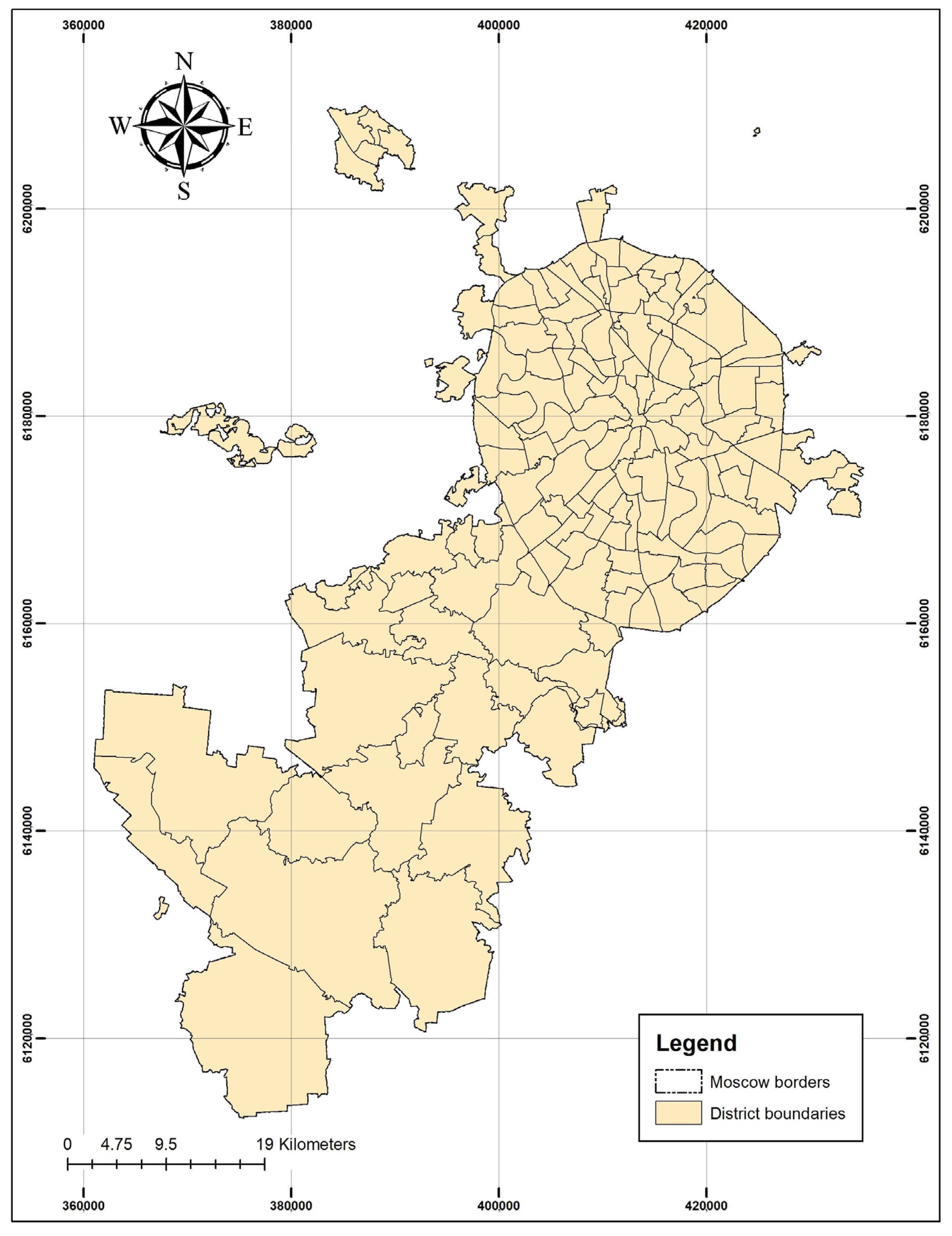
Figure 1. The administrative division layout of the city of Moscow.
Remotesensing 15 03294 g001
Figure 2. Procedure for obtaining high-quality, user-specified Landsat composite mosaic images using the GEE platform.
Remotesensing 15 03294 g002
Figure 3. Workflow for land use classification with the GEE platform.
Remotesensing 15 03294 g003
Figure 4. Landsat spectral index chart from 1997 to 2021.
Remotesensing 15 03294 g004
Figure 5. Land cover of Moscow from 1997 to 2021.
Remotesensing 15 03294 g005
Figure 6. Map of the land cover of Moscow in 1997.
Remotesensing 15 03294 g006
Figure 7. Map of the land cover of Moscow in 2011.
Remotesensing 15 03294 g007
Figure 8. Map of the land cover of Moscow in 2021.
Remotesensing 15 03294 g008
Figure 9. Average daytime temperature for the year.
Remotesensing 15 03294 g009
Figure 10. Average nighttime temperature values of the year.
Remotesensing 15 03294 g010
Figure 11. Map of the average land surface temperature of Moscow for five years.
Remotesensing 15 03294 g011
Figure 12. The temperature of the land surface in Moscow in 2016 year.
Remotesensing 15 03294 g012
Figure 13. The temperature of the land surface in Moscow in 2021.
Remotesensing 15 03294 g013
Figure 14. SUHI categories of Moscow in 2016.
Remotesensing 15 03294 g014
Figure 15. SUHI categories of Moscow in 2021.
Remotesensing 15 03294 g015
Figure 16. Diagram of physicochemical processes in the air [30].
Remotesensing 15 03294 g016
Figure 17. SUHI locations in Moscow in 2021.
Remotesensing 15 03294 g017
Figure 18. PM2.5 concentration schemes in Moscow on 6 June 2019 [43].
Remotesensing 15 03294 g018
Figure 19. The modeling of urban sustainability on the GEE platform using cloud computing.
Remotesensing 15 03294 g019
Table 1. Information on Landsat surface reflectance data can be found on Google Earth Engine (GEE).
Collection NameGEE Image Collection IDData Availabitity
Landsat 5LANDSAT/LT05/C01/T1_SR1 January 1984–5 May 2012
Landsat 7LANDSAT/LE07/C01/T1_SR1 January 1999–April 2022
Landsat 8LANDSAT/LC08/C01/T1_SR11 April 2012–to present
MOD11A2.061MODIS/061/MOD11A218 February 2000–to present
Table 2. Classification of land cover in Moscow.
Time Point199720112021
Water27.0524.6921.70
Urban104.99484.03665.20
Tree2140.981803.941641.02
Bare land213.99174.35159.09
Total area (square km)2487.012487.012487.01
Table 3. Statistics showing the highest average temperature difference between day and night in 5 years.
DateHighest Average Daytime Temperature (°C)Highest Average Night-Time Temperature (°C) Δ t ( ° C )
4 July 201525.8115.5810.23
27 July 201627.5319.028.51
13 August 201726.0916.179.92
28 July 201828.0917.0711.02
2 July 201928.5514.9113.64
Table 4. The threshold values of the urban thermal field variance index (UTFVI) and the ecological evaluation index [25].
UTFVI
(Urban Thermal Field Variance Index)
Urban Heat IslandEcological Evaluation Index
<0.000NoneExcellent
0.000–0.005WeakGood
0.005–0.010MiddleNormal
0.010–0.015StrongBad
0.015–0.020StrongerWorse
0.020StrongestWorst
Disclaimer/Publisher’s Note: The statements, opinions and data contained in all publications are solely those of the individual author(s) and contributor(s) and not of MDPI and/or the editor(s). MDPI and/or the editor(s) disclaim responsibility for any injury to people or property resulting from any ideas, methods, instructions or products referred to in the content.