

Sample Plots Forestry Parameters Verification and Updating Using Airborne LiDAR Data

Abstract
1. Introduction
2. Materials and Methods
2.1. Materials
2.1.1. Study Area
2.1.2. Sample Plot Data
2.1.3. LiDAR Data
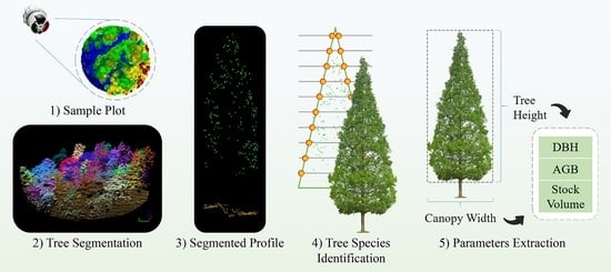
2.2. Methods
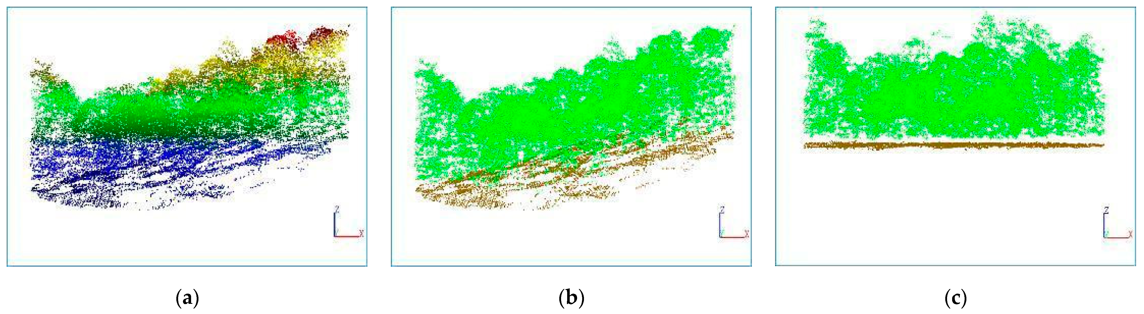
2.2.1. Point Cloud Preprocessing
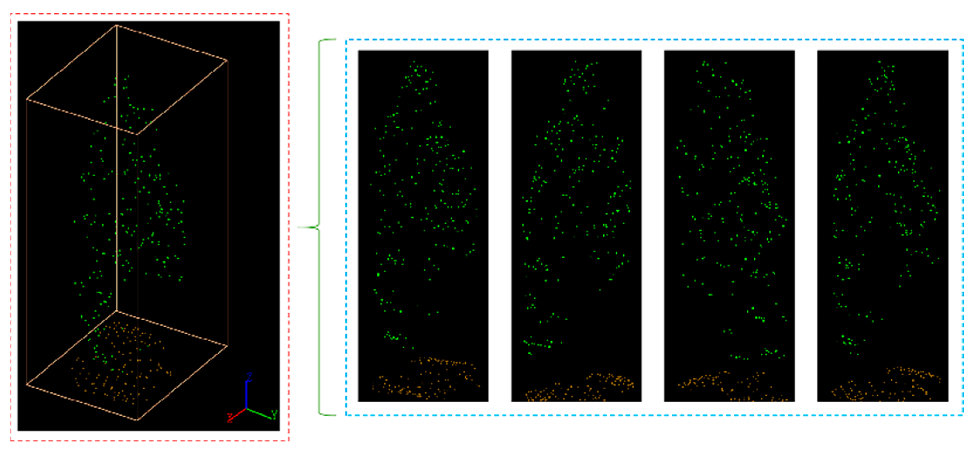
2.2.2. Tree Segmentation
2.2.3. Plot Matching Based on Dominant Trees
2.2.4. Tree Species Identification and Verification
2.2.5. Forestry Parameter Extraction
3. Results
3.1. Ground Point Extraction
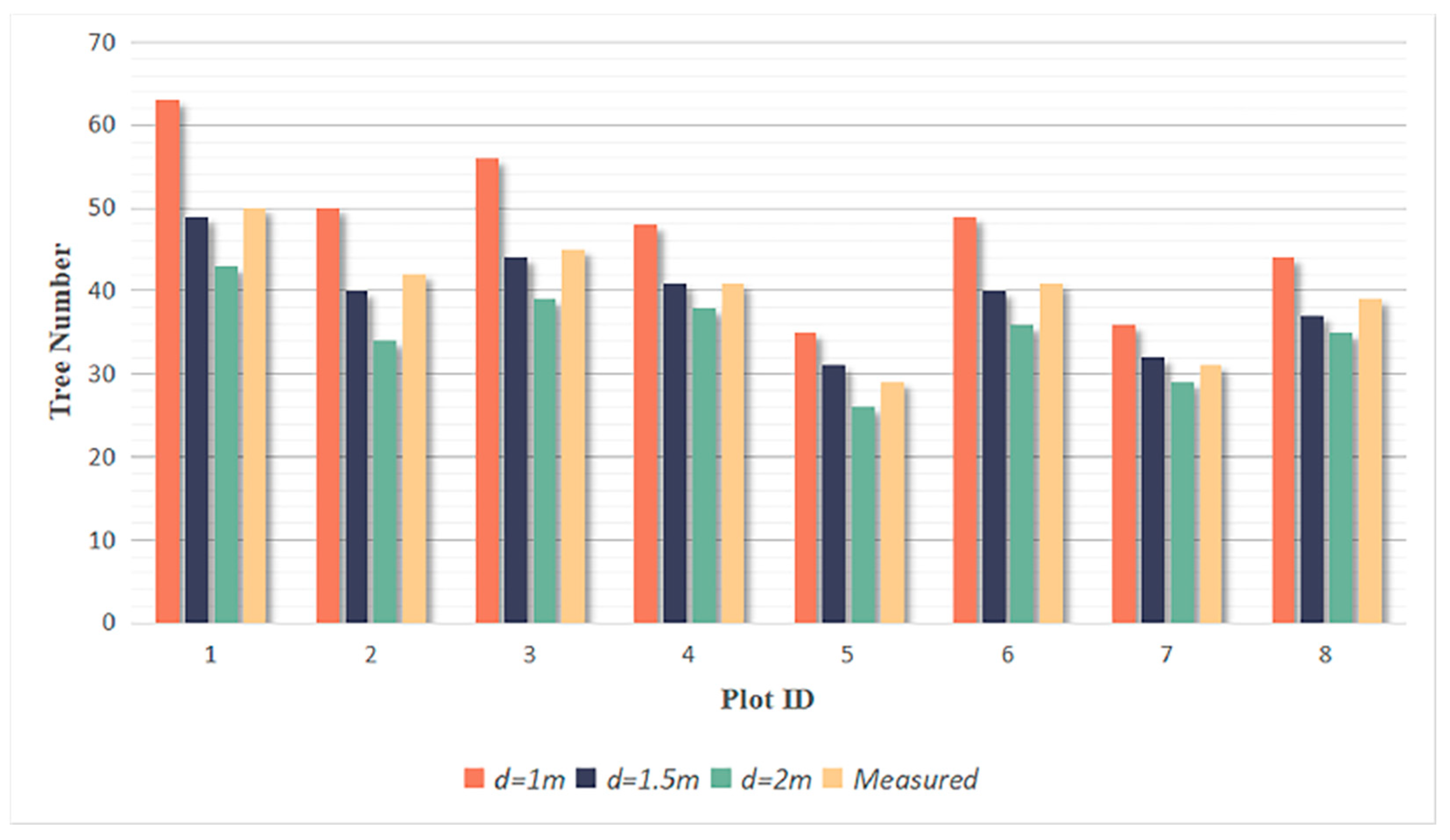
3.2. Tree Segmentation
3.3. Plot Matching and Tree Species Identification
3.4. Forestry Parameters Extraction
4. Discussion
4.1. Tree Segmentation
4.2. Tree Species Identification
4.3. Forestry Parameters Extraction
5. Conclusions
- (1)
- The article uses the PTD algorithm to separate ground and nonground points with an accuracy of more than 95%, achieving excellent separation results and providing a good preparation for the subsequent steps;
- (2)
- The rotating profile algorithm is applied to the tree segmentation, and the oversegmentation and undersegmentation are suppressed when grid size d = 1.5 m. Under this condition, the F-scores of the eight sample plots exceed 0.94, the overall F-score is 0.975, and the overall BA is 0.933;
- (3)
- Using information on tree species from the plot samples, the correspondence between tree species and segmented crowns geometry is established, achieving tree species recognition and information correction based on LIDAR data, with an overall correctness rate of 90.9%;
- (4)
- Based on the updated tree species, tree height, east–west crown width, north–south crown width, DBH, AGB, and stock volume are extracted from the sample plots. R2 of these estimated parameters are 0.893, 0.757, 0.694, 0.840, 0.896 and 0.891, respectively, which strongly correlate with the measured values.
Author Contributions
Funding
Data Availability Statement
Conflicts of Interest
References
- Eckert, S. Improved Forest Biomass and Carbon Estimations Using Texture Measures from WorldView-2 Satellite Data. Remote Sens. 2012, 4, 810–829. [Google Scholar] [CrossRef]
- He, X.; Ren, C.; Chen, L.; Wang, Z.; Zheng, H. The Progress of Forest Ecosystems Monitoring with Remote Sensing Techniques. Sci. Geogr. Sin. 2018, 38, 97–1011. [Google Scholar] [CrossRef]
- Malhi, Y.; Baldocchi, D.D.; Jarvis, P.G. The carbon balance of tropical, temperate and boreal forests. Plant Cell Environ. 1999, 22, 715–740. [Google Scholar] [CrossRef]
- Dong, X.; Li, J.; Chen, H.; Zhao, L.; Zhang, L.; Xing, S. Extraction of individual tree information based on remote sensing images from an Unmanned Aerial Vehicle. J. Remote Sens. 2019, 23, 1269–1280. [Google Scholar] [CrossRef]
- Wang, L.; Yin, H. An Application of New Portable Tree Altimeter DZH-30 in Forest Resources Inventory. For. Resour. Wanagement 2019, 06, 132–136. [Google Scholar] [CrossRef]
- Liu, F.; Tan, C.; Zhang, G.; Liu, J. Estimation of Forest Parameter and Biomass for Individual Pine Trees Using Airborne LiDAR. Trans. Chin. Soc. Agric. Mach. 2013, 44, 219–224, 242. [Google Scholar] [CrossRef]
- Ouma, Y.O. Optimization of Second-Order Grey-Level Texture in High-Resolution Imagery for Statistical Estimation of Above-Ground Biomass. J. Environ. Inform. 2006, 8, 70–85. [Google Scholar] [CrossRef]
- Marshall, M.; Thenkabail, P. Advantage of hyperspectral EO-1 Hyperion over multispectral IKONOS, GeoEye-1, WorldView-2, Landsat ETM+, and MODIS vegetation indices in crop biomass estimation. ISPRS J. Photogramm. Remote Sens. 2015, 108, 205–218. [Google Scholar] [CrossRef]
- Mohammadi, J.; Shataee, S.; Babanezhad, M. Estimation of forest stand volume, tree density and biodiversity using Landsat ETM+Data, comparison of linear and regression tree analyses. Procedia Environ. Sci. 2011, 7, 299–304. [Google Scholar] [CrossRef]
- Franklin, S.E.; Hall, R.J.; Smith, L.; Gerylo, G.R. Discrimination of conifer height, age and crown closure classes using Landsat-5 TM imagery in the Canadian Northwest Territories. Int. J. Remote Sens. 2003, 24, 1823–1834. [Google Scholar] [CrossRef]
- Brown, S.; Pearson, T.; Slaymaker, D.; Ambagis, S.; Moore, N.; Novelo, D.; Sabido, W. Creating a virtual tropical forest from three-dimensional aerial imagery to estimate carbon stocks. Ecol. Appl. 2005, 15, 1083–1095. [Google Scholar] [CrossRef]
- Cloude, S.R.; Papathanassiou, K.P. Forest Vertical Structure Estimation using Coherence Tomography. In Proceedings of the IGARSS 2008—2008 IEEE International Geoscience and Remote Sensing Symposium, Boston, MA, USA, 6–11 July 2008. [Google Scholar] [CrossRef]
- Blomberg, E.; Ferro-Famil, L.; Soja, M.J.; Ulander, L.M.H.; Tebaldini, S. Forest Biomass Retrieval From L-Band SAR Using Tomographic Ground Backscatter Removal. IEEE Geosci. Remote Sens. Lett. 2018, 15, 1030–1034. [Google Scholar] [CrossRef]
- Matasci, G.; Hermosilla, T.; Wulder, M.A.; White, J.C.; Coops, N.C.; Hobart, G.W.; Zald, H.S.J. Large-area mapping of Canadian boreal forest cover, height, biomass and other structural attributes using Landsat composites and lidar plots. Remote Sens. Environ. 2018, 209, 90–106. [Google Scholar] [CrossRef]
- Luckman, A.; Baker, J.; Honzák, M.; Lucas, R. Tropical Forest Biomass Density Estimation Using JERS-1 SAR: Seasonal Variation, Confidence Limits, and Application to Image Mosaics. Remote Sens. Environ. 1998, 63, 126–139. [Google Scholar] [CrossRef]
- Means, J. Use of Large-Footprint Scanning Airborne Lidar to Estimate Forest Stand Characteristics in the Western Cascades of Oregon. Remote Sens. Environ. 1999, 67, 298–308. [Google Scholar] [CrossRef]
- White, J.C.; Wulder, M.A.; Varhola, A.; Vastaranta, M.; Coops, N.C.; Cook, B.D.; Pitt, D.; Woods, M. A best practices guide for generating forest inventory attributes from airborne laser scanning data using an area-based approach. For. Chron. 2013, 89, 722–723. [Google Scholar] [CrossRef]
- Lefsky, M.A.; Cohen, W.B.; Acker, S.A.; Parker, G.G.; Spies, T.A.; Harding, D. Lidar Remote Sensing of the Canopy Structure and Biophysical Properties of Douglas-Fir Western Hemlock Forests. Remote Sens. Environ. 1999, 70, 339–361. [Google Scholar] [CrossRef]
- Temesgen, H.; Zhang, C.H.; Zhao, X.H. Modelling tree height–diameter relationships in multi-species and multi-layered forests: A large observational study from Northeast China. For. Ecol. Manag. 2014, 316, 78–89. [Google Scholar] [CrossRef]
- Schmidt, M.; Kiviste, A.; von Gadow, K. A spatially explicit height–diameter model for Scots pine in Estonia. Eur. J. For. Res. 2010, 130, 303–315. [Google Scholar] [CrossRef]
- Zheng, J.; Zang, H.; Yin, S.; Sun, N.; Zhu, P.; Han, Y.; Kang, H.; Liu, C. Modeling height-diameter relationship for artificial monoculture Metasequoia glyptostroboides in sub-tropic coastal megacity Shanghai, China. Urban For. Urban Green. 2018, 34, 226–232. [Google Scholar] [CrossRef]
- Ng’andwe, P.; Chungu, D.; Yambayamba, A.M.; Chilambwe, A. Modeling the height-diameter relationship of planted Pinus kesiya in Zambia. For. Ecol. Manag. 2019, 447, 1–11. [Google Scholar] [CrossRef]
- Hyyppä, J.; Yu, X.; Hyyppä, H.; Vastaranta, M.; Holopainen, M.; Kukko, A.; Kaartinen, H.; Jaakkola, A.; Vaaja, M.; Koskinen, J.; et al. Advances in Forest Inventory Using Airborne Laser Scanning. Remote Sens. 2012, 4, 1190–1207. [Google Scholar] [CrossRef]
- Kaartinen, H.; Hyyppä, J.; Yu, X.; Vastaranta, M.; Hyyppä, H.; Kukko, A.; Holopainen, M.; Heipke, C.; Hirschmugl, M.; Morsdorf, F.; et al. An International Comparison of Individual Tree Detection and Extraction Using Airborne Laser Scanning. Remote Sens. 2012, 4, 950–974. [Google Scholar] [CrossRef]
- Kampa, K.; Slatton, K.C. An adaptive multiscale filter for segmenting vegetation in ALSM data. In Proceedings of the IGARSS 2004. 2004 IEEE International Geoscience and Remote Sensing Symposium, Anchorage, AK, USA, 20–24 September 2004. [Google Scholar] [CrossRef]
- Lee, H.; Slatton, K.C.; Roth, B.E.; Cropper, W.P. Adaptive clustering of airborne LiDAR data to segment individual tree crowns in managed pine forests. Int. J. Remote Sens. 2010, 31, 117–139. [Google Scholar] [CrossRef]
- Mei, C.; Durrieu, S. Tree crown delineation from digital elevation models and high resolution imagery. Proc. IAPRS 2004, 36, 218–223. [Google Scholar]
- Chen, Q.; Baldocchi, D.; Gong, P.; Kelly, M. Isolating Individual Trees in a Savanna Woodland Using Small Footprint Lidar Data. Photogramm. Eng. Remote Sens. 2006, 72, 923–932. [Google Scholar] [CrossRef]
- Tang, F.; Zhang, X.; Liu, J. Segmentation of tree crown model with complex structure from airborne LIDAR data. In Geoinformatics 2007: Remotely Sensed Data and Information; SPIE: Bellingham, DC, USA, 2007. [Google Scholar] [CrossRef]
- Leckie, D.; Gougeon, F.; Hill, D.; Quinn, R.; Armstrong, L.; Shreenan, R. Combined high-density lidar and multispectral imagery for individual tree crown analysis. Can. J. Remote Sens. 2003, 29, 633–649. [Google Scholar] [CrossRef]
- Liu, T.; Im, J.; Quackenbush, L.J. A novel transferable individual tree crown delineation model based on Fishing Net Dragging and boundary classification. ISPRS J. Photogramm. Remote Sens. 2015, 110, 34–47. [Google Scholar] [CrossRef]
- Reitberger, J.; Schnörr, C.; Krzystek, P.; Stilla, U. 3D segmentation of single trees exploiting full waveform LIDAR data. ISPRS J. Photogramm. Remote Sens. 2009, 64, 561–574. [Google Scholar] [CrossRef]
- Lu, X.; Guo, Q.; Li, W.; Flanagan, J. A bottom-up approach to segment individual deciduous trees using leaf-off lidar point cloud data. ISPRS J. Photogramm. Remote Sens. 2014, 94, 1–12. [Google Scholar] [CrossRef]
- Wang, Y.; Weinacker, H.; Koch, B. A Lidar Point Cloud Based Procedure for Vertical Canopy Structure Analysis And 3D Single Tree Modelling in Forest. Sensors 2008, 8, 3938–3951. [Google Scholar] [CrossRef]
- Morsdorf, F.; Meier, E.H.; Allgöwer, B.; Nüesch, D. Clustering in airborne laser scanning raw data for segmentation of single trees. Int. Arch. Photogramm. Remote Sens. Spat. Inf. Sci. 2003, 34, W13. [Google Scholar]
- Li, W.; Guo, Q.; Jakubowski, M.K.; Kelly, M. A New Method for Segmenting Individual Trees from the Lidar Point Cloud. Photogramm. Eng. Remote Sens. 2012, 78, 75–84. [Google Scholar] [CrossRef]
- Chen, X.; Jiang, K.; Zhu, Y.; Wang, X.; Yun, T. Individual Tree Crown Segmentation Directly from UAV-Borne LiDAR Data Using the PointNet of Deep Learning. Forests 2021, 12, 131. [Google Scholar] [CrossRef]
- Yan, W.; Guan, H.; Cao, L.; Yu, Y.; Li, C.; Lu, J. A Self-Adaptive Mean Shift Tree-Segmentation Method Using UAV LiDAR Data. Remote Sens. 2020, 12, 515. [Google Scholar] [CrossRef]
- Qian, C.; Yao, C.; Ma, H.; Xu, J.; Wang, J. Tree Species Classification Using Airborne LiDAR Data Based on Individual Tree Segmentation and Shape Fitting. Remote Sens. 2023, 15, 406. [Google Scholar] [CrossRef]
- Holmgren, J.; Persson, Å. Identifying species of individual trees using airborne laser scanner. Remote Sens. Environ. 2004, 90, 415–423. [Google Scholar] [CrossRef]
- Othmani, A.; Lew Yan Voon, L.F.C.; Stolz, C.; Piboule, A. Single tree species classification from Terrestrial Laser Scanning data for forest inventory. Pattern Recognit. Lett. 2013, 34, 2144–2150. [Google Scholar] [CrossRef]
- Lin, Y.; Hyyppä, J. A comprehensive but efficient framework of proposing and validating feature parameters from airborne LiDAR data for tree species classification. Int. J. Appl. Earth Obs. Geoinf. 2016, 46, 45–55. [Google Scholar] [CrossRef]
- Kim, S.; McGaughey, R.J.; Andersen, H.-E.; Schreuder, G. Tree species differentiation using intensity data derived from leaf-on and leaf-off airborne laser scanner data. Remote Sens. Environ. 2009, 113, 1575–1586. [Google Scholar] [CrossRef]
- Ørka, H.O.; Næsset, E.; Bollandsås, O.M. Classifying species of individual trees by intensity and structure features derived from airborne laser scanner data. Remote Sens. Environ. 2009, 113, 1163–1174. [Google Scholar] [CrossRef]
- Kashani, A.; Olsen, M.; Parrish, C.; Wilson, N. A Review of LIDAR Radiometric Processing: From Ad Hoc Intensity Correction to Rigorous Radiometric Calibration. Sensors 2015, 15, 28099–28128. [Google Scholar] [CrossRef]
- Qin, H.; Zhou, W.; Yao, Y.; Wang, W. Individual tree segmentation and tree species classification in subtropical broadleaf forests using UAV-based LiDAR, hyperspectral, and ultrahigh-resolution RGB data. Remote Sens. Environ. 2022, 280, 113143. [Google Scholar] [CrossRef]
- Solodukhin, V.I.; Zukov, A.J.; Mazugin, I.N. Laser aerial profiling of a forest. Lew NIILKh Leningr. Lesn. Khozyaistvo 1977, 10, 53–58. [Google Scholar]
- Shrestha, R.; Wynne, R.H. Estimating Biophysical Parameters of Individual Trees in an Urban Environment Using Small Footprint Discrete-Return Imaging Lidar. Remote Sens. 2012, 4, 484–508. [Google Scholar] [CrossRef]
- Bortolot, Z.J.; Wynne, R.H. Estimating forest biomass using small footprint LiDAR data: An individual tree-based approach that incorporates training data. ISPRS J. Photogramm. Remote Sens. 2005, 59, 342–360. [Google Scholar] [CrossRef]
- Wang, D.; Xin, X.; Shao, Q.; Brolly, M.; Zhu, Z.; Chen, J. Modeling Aboveground Biomass in Hulunber Grassland Ecosystem by Using Unmanned Aerial Vehicle Discrete Lidar. Sensors 2017, 17, 180. [Google Scholar] [CrossRef] [PubMed]
- García, M.; Riaño, D.; Chuvieco, E.; Danson, F.M. Estimating biomass carbon stocks for a Mediterranean forest in central Spain using LiDAR height and intensity data. Remote Sens. Environ. 2010, 114, 816–830. [Google Scholar] [CrossRef]
- Donoghue, D.; Watt, P.; Cox, N.; Wilson, J. Remote sensing of species mixtures in conifer plantations using LiDAR height and intensity data. Remote Sens. Environ. 2007, 110, 509–522. [Google Scholar] [CrossRef]
- Jin, J.; Yue, C.; Li, C.; Gu, L.; Luo, H.; Zhu, B. Estimation on Forest Volume Based on ALS Data and Dummy Variable Technology. For. Resour. Wanagement 2021, 01, 77–85. [Google Scholar] [CrossRef]
- PANG, Y.; LI, Z.-Y. Inversion of biomass components of the temperate forest using airborne Lidar technology in Xiaoxing’an Mountains, Northeastern of China. Chin. J. Plant Ecol. 2013, 36, 1095–1105. [Google Scholar] [CrossRef]
- Jia-Jia, J.; Xian-Quan, W.; Fa-Jie, D. An Effective Frequency-Spatial Filter Method to Restrain the Interferences for Active Sensors Gain and Phase Errors Calibration. IEEE Sens. J. 2016, 16, 7713–7719. [Google Scholar] [CrossRef]
- Axelsson, P. Processing of laser scanner data—Algorithms and applications. ISPRS J. Photogramm. Remote Sens. 1999, 54, 138–147. [Google Scholar] [CrossRef]
- Goutte, C.; Gaussier, E. A Probabilistic Interpretation of Precision, Recall and F-Score, with Implication for Evaluation. Adv. Inf. Retr. 2005, 3408, 345–359. [Google Scholar] [CrossRef]
- Brodersen, K.H.; Ong, C.S.; Stephan, K.E.; Buhmann, J.M. The Balanced Accuracy and Its Posterior Distribution. In Proceedings of the 2010 20th International Conference on Pattern Recognition, Istanbul, Turkey, 23–26 August 2010. [Google Scholar] [CrossRef]
- Goodenough, D.G.; Chen, H.; Dyk, A.; Richardson, A.; Hobart, G. Data Fusion Study Between Polarimetric SAR, Hyperspectral and Lidar Data for Forest Information. In Proceedings of the IGARSS 2008—2008 IEEE International Geoscience and Remote Sensing Symposium, Boston, MA, USA, 6–11 July 2008. [Google Scholar] [CrossRef]
- Alonzo, M.; Bookhagen, B.; Roberts, D.A. Urban tree species mapping using hyperspectral and lidar data fusion. Remote Sens. Environ. 2014, 148, 70–83. [Google Scholar] [CrossRef]
- Hinton, G.E.; Osindero, S.; Teh, Y.-W. A Fast Learning Algorithm for Deep Belief Nets. Neural Comput. 2006, 18, 1527–1554. [Google Scholar] [CrossRef] [PubMed]
- Yang, Q.; Su, Y.; Jin, S.; Kelly, M.; Hu, T.; Ma, Q.; Li, Y.; Song, S.; Zhang, J.; Xu, G.; et al. The Influence of Vegetation Characteristics on Individual Tree Segmentation Methods with Airborne LiDAR Data. Remote Sens. 2019, 11, 2880. [Google Scholar] [CrossRef]
- Ma, K.; Chen, Z.; Fu, L.; Tian, W.; Jiang, F.; Yi, J.; Du, Z.; Sun, H. Performance and Sensitivity of Individual Tree Segmentation Methods for UAV-LiDAR in Multiple Forest Types. Remote Sens. 2022, 14, 298. [Google Scholar] [CrossRef]
- Ma, K.; Xiong, Y.; Jiang, F.; Chen, S.; Sun, H. A Novel Vegetation Point Cloud Density Tree-Segmentation Model for Overlapping Crowns Using UAV LiDAR. Remote Sens. 2021, 13, 1442. [Google Scholar] [CrossRef]
- Liu, Y.; Zhang, X.; Ma, Z.; Dong, N.; Xie, D.; Li, R.; Johnston, D.M.; Gao, Y.G.; Li, Y.; Lei, Y. Developing a more accurate method for individual plant segmentation of urban tree and shrub communities using LiDAR technology. Landsc. Res. 2022, 48, 313–330. [Google Scholar] [CrossRef]
- Zou, X.; Cheng, M.; Wang, C.; Xia, Y.; Li, J. Tree Classification in Complex Forest Point Clouds Based on Deep Learning. IEEE Geosci. Remote Sens. Lett. 2017, 14, 2360–2364. [Google Scholar] [CrossRef]
- Zhong, H.; Lin, W.; Liu, H.; Ma, N.; Liu, K.; Cao, R.; Wang, T.; Ren, Z. Identification of tree species based on the fusion of UAV hyperspectral image and LiDAR data in a coniferous and broad-leaved mixed forest in Northeast China. Front. Plant Sci. 2022, 13, 964769. [Google Scholar] [CrossRef] [PubMed]
- Onishi, M.; Ise, T. Explainable identification and mapping of trees using UAV RGB image and deep learning. Sci. Rep. 2021, 11, 903. [Google Scholar] [CrossRef] [PubMed]
- Liu, M.; Han, Z.; Chen, Y.; Liu, Z.; Han, Y. Tree species classification of LiDAR data based on 3D deep learning. Measurement 2021, 177, 109301. [Google Scholar] [CrossRef]


| Plot ID | 1 | 2 | 3 | 4 | 5 | 6 | 7 | 8 | |
|---|---|---|---|---|---|---|---|---|---|
| Number of Trees | 50 | 42 | 45 | 41 | 29 | 41 | 31 | 39 | |
| Dominant Tree Species | pine | linden | linden | linden | linden | poplar | oak | linden | |
| Mean Tree Height (m) | 14.5 | 13.5 | 16.9 | 8.2 | 14.3 | 16.4 | 13.8 | 14.3 | |
| Standard Deviation of Tree Height (m) | 4.99 | 3.64 | 2.87 | 2.91 | 4.33 | 6.01 | 5.17 | 4.62 | |
| Mean DBH (cm) | 18.6 | 17.8 | 16.9 | 10.5 | 20.7 | 20.8 | 20.1 | 18.3 | |
| Standard Deviation of DBH (cm) | 8.56 | 6.99 | 4.66 | 5.25 | 5.93 | 10.27 | 11.25 | 7.19 | |
| Mean HUB (m) | 4.8 | 3.6 | 3.2 | 2.3 | 4.0 | 5.1 | 3.6 | 4.6 | |
| Standard Deviation of HUB (m) | 2.91 | 2.01 | 1.59 | 0.92 | 2.03 | 3.42 | 1.47 | 2.67 | |
| Mean Crown Width (m) | East–West | 2.72 | 2.49 | 2.61 | 2.27 | 2.60 | 2.83 | 2.82 | 2.27 |
| North–South | 2.72 | 2.10 | 2.31 | 2.16 | 1.82 | 2.97 | 2.20 | 1.98 | |
| Cumulative Stock Volume (m3) | 14.4 | 9.7 | 8.1 | 3.5 | 9.5 | 14.6 | 9.8 | 9.1 | |
| Cumulative AGB (t/ha) | 8390.7 | 7743.4 | 5879.0 | 2239.1 | 7158.5 | 8565.2 | 9342.1 | 7717.1 | |
| Properties of the Point Cloud Data | Contents |
|---|---|
| Flight Platform | Cessna 208b aircraft |
| LiDAR Scanner Type | riegl-vq-1560i |
| Average Height Above Ground Level (m) | 1000 |
| Overlap of flight lines | 20% |
| Horizontal accuracy (cm) | 15~25 |
| Vertical accuracy (cm) | 15 |
| Point density (pts/m2) | 20 |
| Forestry Parameters | Acquisition Method | Estimating Equation Factors |
|---|---|---|
| Tree Height | Direct measurement | / |
| crown width | Segmented Point Cloud Measurements | / |
| DBH | Growth Equation Estimation | Tree Height |
| AGB | Growth Equation Estimation | Tree Height, DBH |
| Stock Volume | Growth Equation Estimation | DBH |
| Tree Species | Factor | Estimation Formula | Applicable Condition (H) | Parameters | |
|---|---|---|---|---|---|
| a | b | ||||
| Pine | H | DBH = exp(a + b∗H) | 2–36.5 | 1.646 | 0.081 |
| Oak | H | DBH = exp(a + b∗H) | 8.8–27.4 | 1.138 | 0.111 |
| Birch | H | DBH = exp(a + b∗H) | 5–24.2 | 1.043 | 0.116 |
| Elm | H | DBH = exp(a + b∗H) | 3–25.9 | 1.040 | 0.121 |
| Linden | H | DBH = exp(a + b∗H) | 8.2–29.9 | 0.733 | 0.129 |
| Poplar | H | DBH = exp(a + b∗H) | 4.8–30.1 | 1.171 | 0.110 |
| Maple | H | DBH = exp(a + b∗H) | 5–22.4 | 0.958 | 0.135 |
| Tree Species | Factors | Estimation Formula | Parameters | ||
|---|---|---|---|---|---|
| a | b | c | |||
| Pine | H, DBH | AGB = aDBHbHc | 0.120 | 2.064 | 0.383 |
| Oak | H, DBH | AGB = a(DBH2H)b | 0.020 | 1.039 | / |
| Birch | H, DBH | AGB = a(DBH2H)b | 0.020 | 1.039 | / |
| Elm | H, DBH | AGB = a(DBH2H)b | 0.020 | 1.039 | / |
| Linden | H, DBH | AGB = a(DBH2H)b | 0.020 | 1.039 | / |
| Poplar | DBH | AGB = aDBHb | 0.022 | 2.737 | / |
| Maple | H, DBH | AGB = a(DBH2H)b | 0.020 | 1.039 | / |
| Tree Species | a | b | c | d | e | k |
|---|---|---|---|---|---|---|
| Pine | 5.09 × 10⁻⁵ | 1.809 | 1.101 | 48.429 | −2385.550 | 50 |
| Oak | 4.07 × 10⁻⁵ | 1.719 | 1.253 | 23.804 | −240.081 | 8 |
| Birch & Poplar | 4.06 × 10⁻⁵ | 1.835 | 1.113 | 29.850 | −439.555 | 14 |
| Elm | 3.63 × 10⁻⁵ | 1.819 | 1.173 | 26.744 | −472.502 | 18 |
| Linden | 3.55 × 10⁻⁵ | 1.767 | 1.243 | 27.297 | −384.328 | 13 |
| Maple | 4.25 × 10⁻⁵ | 1.783 | 1.140 | 22.511 | −258.117 | 11 |
| Plot ID | Type I Error | Type II Error | Separation Accuracy | Overall Accuracy |
|---|---|---|---|---|
| 1 | 47 | 44 | 98.2% | 97.1% |
| 2 | 46 | 44 | 97.9% | |
| 3 | 120 | 125 | 95.1% | |
| 4 | 69 | 54 | 97.5% | |
| 5 | 91 | 104 | 96.2% | |
| 6 | 72 | 55 | 97.1% | |
| 7 | 68 | 66 | 96.4% | |
| 8 | 6 | 46 | 97.2% |
| Plot ID | Real Number | d = 1 m | d = 1.5 m | d = 2 m | |||||||||
|---|---|---|---|---|---|---|---|---|---|---|---|---|---|
| TP | FN | FP | TN | TP | FN | FP | TN | TP | FN | FP | TN | ||
| 1 | 50 | 49 | 1 | 14 | 19 | 47 | 3 | 2 | 12 | 42 | 8 | 1 | 7 |
| 2 | 42 | 41 | 1 | 9 | 13 | 40 | 2 | 0 | 5 | 34 | 8 | 0 | 3 |
| 3 | 45 | 45 | 0 | 11 | 14 | 44 | 1 | 0 | 8 | 39 | 6 | 0 | 4 |
| 4 | 41 | 41 | 0 | 7 | 8 | 40 | 1 | 1 | 4 | 37 | 4 | 1 | 3 |
| 5 | 29 | 29 | 0 | 6 | 10 | 29 | 0 | 2 | 5 | 25 | 4 | 1 | 4 |
| 6 | 41 | 41 | 0 | 8 | 12 | 40 | 1 | 0 | 9 | 36 | 5 | 0 | 5 |
| 7 | 31 | 31 | 0 | 5 | 6 | 31 | 0 | 1 | 4 | 29 | 2 | 0 | 2 |
| 8 | 39 | 39 | 0 | 5 | 9 | 37 | 2 | 0 | 6 | 35 | 4 | 0 | 3 |
| All | 318 | 316 | 2 | 65 | 91 | 308 | 10 | 6 | 53 | 277 | 41 | 3 | 31 |
| Plot ID | Real Number | d = 1 m | d = 1.5 m | d = 2 m | |||||||||
|---|---|---|---|---|---|---|---|---|---|---|---|---|---|
| r | p | F | BA | r | p | F | BA | r | p | F | BA | ||
| 1 | 50 | 0.980 | 0.778 | 0.867 | 0.778 | 0.940 | 0.959 | 0.949 | 0.899 | 0.840 | 0.977 | 0.903 | 0.858 |
| 2 | 42 | 0.976 | 0.820 | 0.891 | 0.784 | 0.952 | 1.000 | 0.976 | 0.976 | 0.810 | 1.000 | 0.895 | 0.905 |
| 3 | 45 | 1.000 | 0.804 | 0.891 | 0.780 | 0.978 | 1.000 | 0.989 | 0.989 | 0.867 | 1.000 | 0.929 | 0.933 |
| 4 | 41 | 1.000 | 0.854 | 0.921 | 0.767 | 0.976 | 0.976 | 0.976 | 0.888 | 0.902 | 0.973 | 0.937 | 0.826 |
| 5 | 29 | 1.000 | 0.829 | 0.906 | 0.813 | 1.000 | 0.935 | 0.967 | 0.857 | 0.862 | 0.962 | 0.909 | 0.831 |
| 6 | 41 | 1.000 | 0.837 | 0.911 | 0.800 | 0.976 | 1.000 | 0.988 | 0.988 | 0.878 | 1.000 | 0.935 | 0.939 |
| 7 | 31 | 1.000 | 0.861 | 0.925 | 0.773 | 1.000 | 0.969 | 0.984 | 0.900 | 0.935 | 1.000 | 0.967 | 0.968 |
| 8 | 39 | 1.000 | 0.886 | 0.940 | 0.821 | 0.949 | 1.000 | 0.974 | 0.974 | 0.897 | 1.000 | 0.946 | 0.949 |
| All | 318 | 0.994 | 0.829 | 0.904 | 0.789 | 0.969 | 0.981 | 0.975 | 0.933 | 0.871 | 0.989 | 0.926 | 0.891 |
| Plot ID | 1 | 2 | 3 | 4 | 5 | 6 | 7 | 8 |
|---|---|---|---|---|---|---|---|---|
| Matching Degree | 92.1% | 90.5% | 91.7% | 94.2% | 93.2% | 91.8% | 92.5% | 93.7% |
| Deviation Value | 6.32 m | 7.13 m | 6.57 m | 4.63 m | 5.78 m | 7.54 m | 5.84 m | 6.77 m |
| Tree Species | Actual Number | Number of Selected | Number of Profiles |
|---|---|---|---|
| Pine | 40 | 20 | 80 |
| Oak | 25 | 10 | 40 |
| Birch | 14 | 8 | 32 |
| Elm | 19 | 8 | 32 |
| Linden | 114 | 50 | 200 |
| Poplar | 19 | 10 | 40 |
| Maple | 45 | 20 | 80 |
| Tree Species | Correct Classification | Type I Error 1 | Type II Error 2 | Corrected Tree Number | Correct Rate | Overall Correct Rate |
|---|---|---|---|---|---|---|
| Pine | 39 | 1 | 2 | 3 | 100% | 90.9% |
| Oak | 25 | 0 | 2 | 2 | 100% | |
| Birch | 14 | 0 | 1 | 1 | 100% | |
| Elm | 17 | 2 | 1 | 3 | 100% | |
| Linden | 107 | 7 | 0 | 6 | 85.7% | |
| Poplar | 18 | 1 | 1 | 2 | 100% | |
| Maple | 45 | 0 | 3 | 2 | 66.7% | |
| Others | 32 | 0 | 1 | 1 | 100% |
| Collected | Pine | Oak | Birch | Elm | Linden | Polar | Maple | Others | CR 1 | |
|---|---|---|---|---|---|---|---|---|---|---|
| Estimated | ||||||||||
| Pine | 39 | 0 | 0 | 1 | 0 | 0 | 0 | 0 | 100% | |
| Oak | 0 | 25 | 0 | 0 | 0 | 0 | 0 | 0 | 100% | |
| Birch | 0 | 0 | 14 | 0 | 0 | 0 | 0 | 0 | 100% | |
| Elm | 1 | 0 | 0 | 17 | 0 | 0 | 1 | 0 | 100% | |
| Linden | 1 | 2 | 1 | 0 | 107 | 1 | 1 | 1 | 87.5% | |
| Poplar | 0 | 0 | 0 | 0 | 0 | 18 | 1 | 0 | 100% | |
| Maple | 0 | 0 | 0 | 0 | 0 | 0 | 45 | 0 | 66.7% | |
| Others | 0 | 0 | 0 | 0 | 0 | 0 | 0 | 32 | 100% | |
| Parameters | Tree Height | Crown Width | DBH | AGB | Stock Volume | |
|---|---|---|---|---|---|---|
| East–West | North–South | |||||
| R2 | 0.893 | 0.757 | 0.694 | 0.840 | 0.896 | 0.891 |
| RMSE | 1.793 | 0.719 | 0.638 | 3.735 | 70.914 | 0.090 |
| MAE | 1.465 | 0.575 | 0.511 | 3.015 | 48.875 | 0.066 |
| Method | Data | Area | r | p | F |
|---|---|---|---|---|---|
| WA | Lidar data | Inner Mongolia, China | 0.76 | 0.87 | 0.81 |
| VPCDM | Lidar data | Inner Mongolia, China | 0.81 | 0.78 | 0.80 |
| bottom-up | Lidar data | Pennsylvania | 0.84 | 0.97 | 0.90 |
| M-CSP | Lidar data | Zhengzhou city, China | 0.842 | 0.953 | 0.886 |
| WST-Ncut | LiDAR, hyperspectral, and ultrahigh-resolution RGB data | Shenzhen City, China | 0.95 | 0.86 | 0.91 |
| RPAA | Lidar data | northeast China | 0.969 | 0.981 | 0.975 |
Disclaimer/Publisher’s Note: The statements, opinions and data contained in all publications are solely those of the individual author(s) and contributor(s) and not of MDPI and/or the editor(s). MDPI and/or the editor(s) disclaim responsibility for any injury to people or property resulting from any ideas, methods, instructions or products referred to in the content. |
© 2023 by the authors. Licensee MDPI, Basel, Switzerland. This article is an open access article distributed under the terms and conditions of the Creative Commons Attribution (CC BY) license (https://creativecommons.org/licenses/by/4.0/).
Share and Cite
Wang, J.; Yao, C.; Ma, H.; Xu, J.; Qian, C. Sample Plots Forestry Parameters Verification and Updating Using Airborne LiDAR Data. Remote Sens. 2023, 15, 3060. https://doi.org/10.3390/rs15123060
Wang J, Yao C, Ma H, Xu J, Qian C. Sample Plots Forestry Parameters Verification and Updating Using Airborne LiDAR Data. Remote Sensing. 2023; 15(12):3060. https://doi.org/10.3390/rs15123060
Chicago/Turabian StyleWang, Jie, Chunjing Yao, Hongchao Ma, Junhao Xu, and Chen Qian. 2023. "Sample Plots Forestry Parameters Verification and Updating Using Airborne LiDAR Data" Remote Sensing 15, no. 12: 3060. https://doi.org/10.3390/rs15123060
APA StyleWang, J., Yao, C., Ma, H., Xu, J., & Qian, C. (2023). Sample Plots Forestry Parameters Verification and Updating Using Airborne LiDAR Data. Remote Sensing, 15(12), 3060. https://doi.org/10.3390/rs15123060