

NSKY-CD: A System for Cloud Detection Based on Night Sky Brightness and Sky Temperature


Abstract
1. Introduction
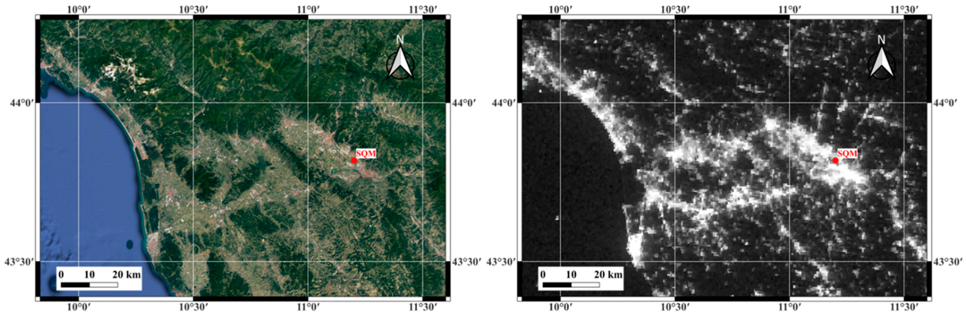
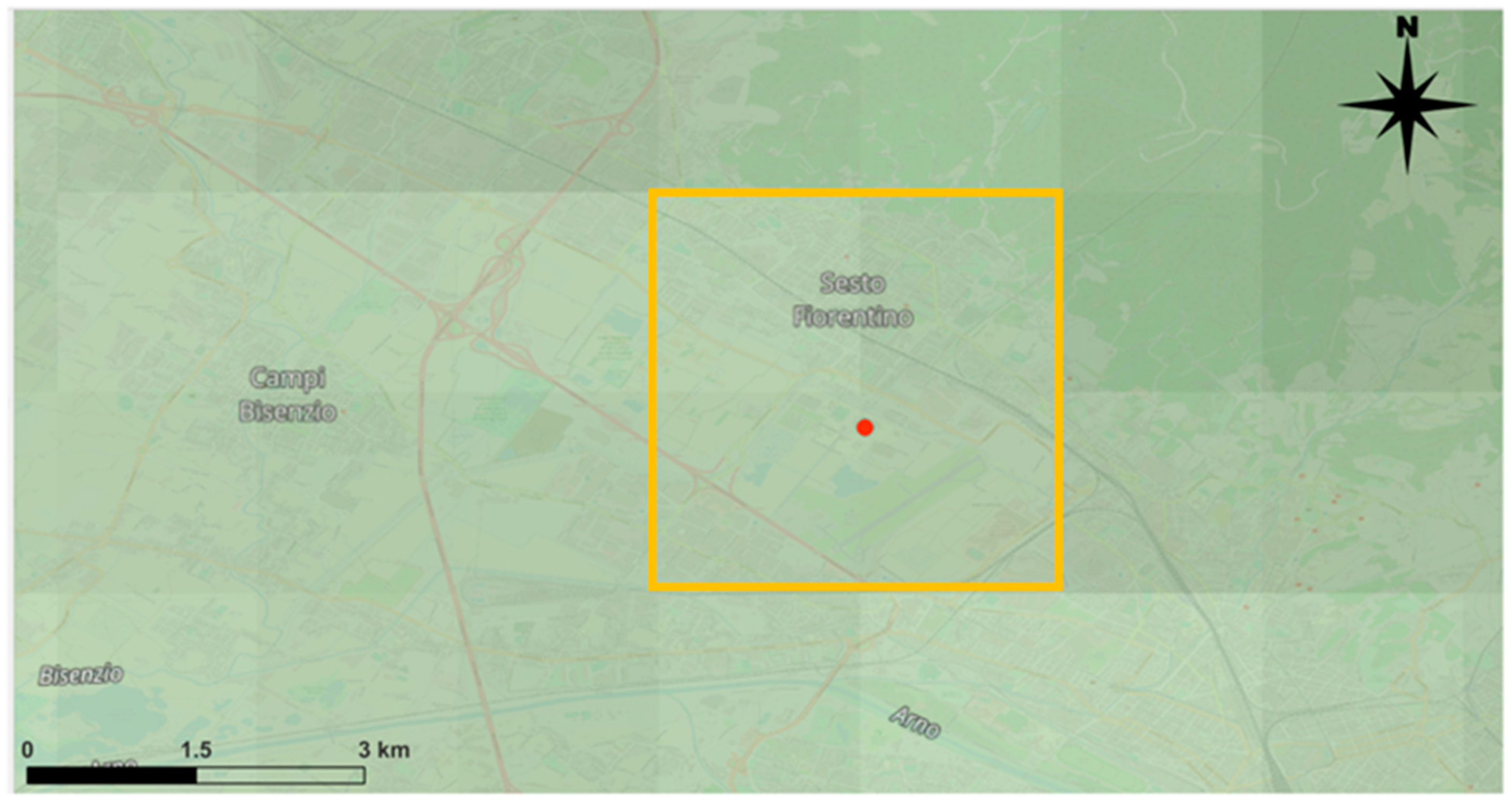
2. Materials and Methods
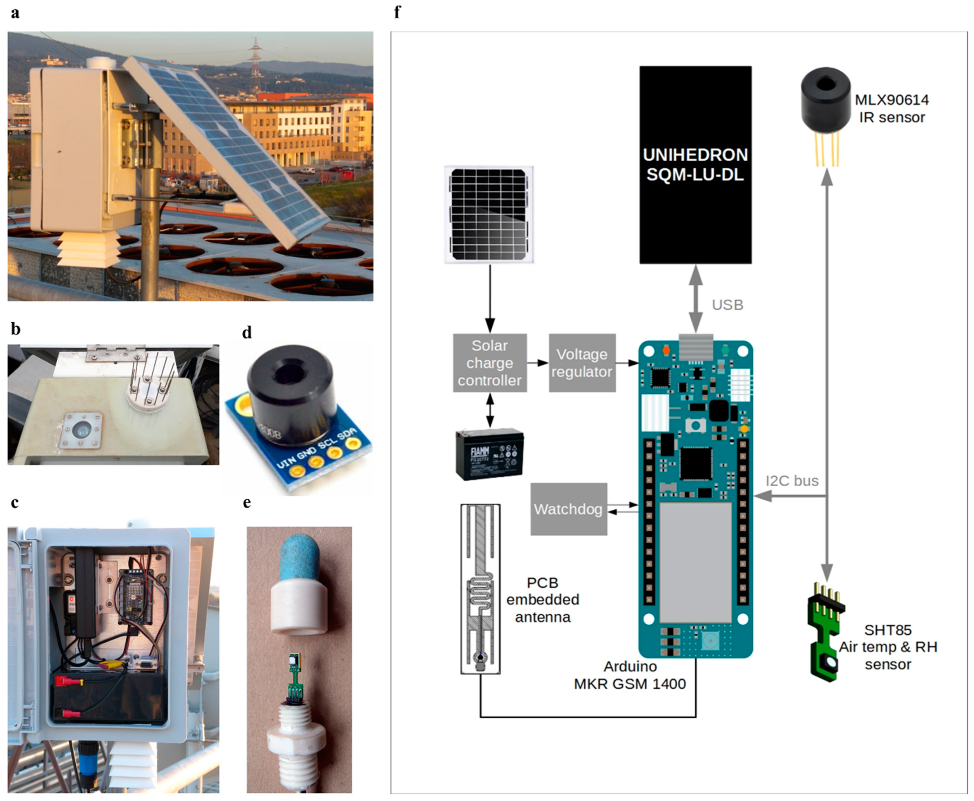
2.1. Description of the System
2.2. Data Analysis
3. Results
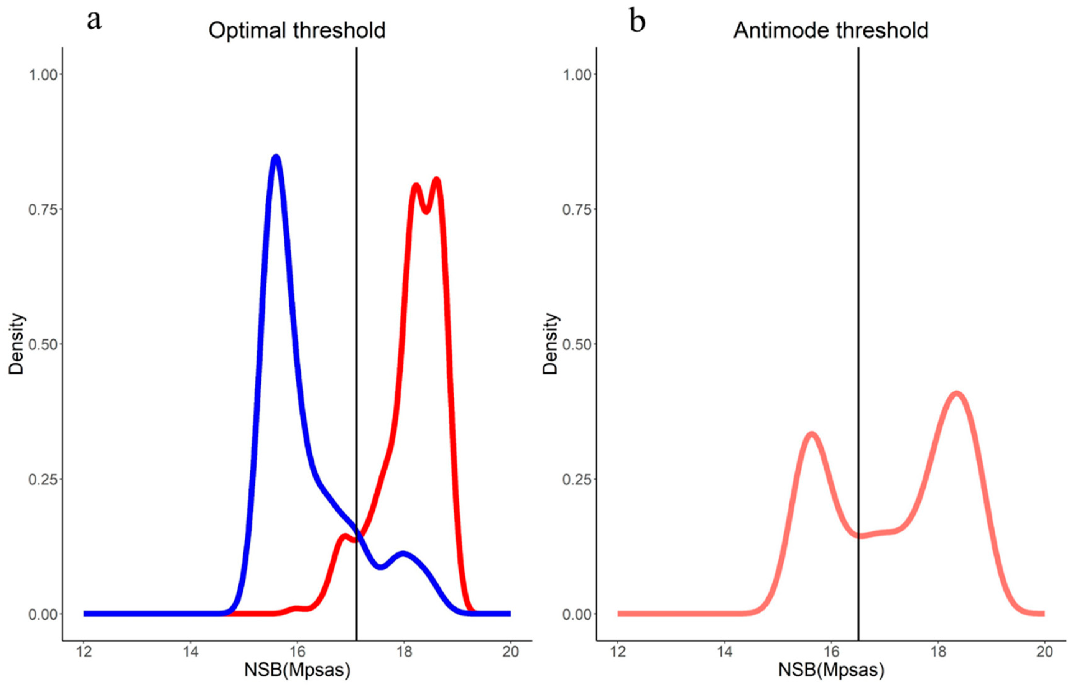
Cloud Detection Accuracy
4. Discussion
5. Conclusions
Author Contributions
Funding
Data Availability Statement
Acknowledgments
Conflicts of Interest
References
- Kyba, C.C.; Tong, K.P.; Bennie, J.; Birriel, I.; Birriel, J.J.; Cool, A.; Gaston, K.J. Worldwide variations in artificial skyglow. Sci. Rep. 2015, 5, 8409. [Google Scholar] [CrossRef] [PubMed]
- Falchi, F.; Cinzano, P.; Duriscoe, D.; Kyba, C.C.M.; Elvidge, C.D.; Baugh, K.; Portnov, B.A.; Rybnikova, N.A.; Furgoni, R. The new world atlas of artificial night sky brightness. Sci. Adv. 2016, 2, e1600377. [Google Scholar] [CrossRef] [PubMed]
- Duriscoe, D.; Luginbuhl, C.; Elvidge, C. The relation of outdoor lighting characteristics to sky glow from distant cities. Light. Res. Technol. 2014, 46, 35–49. [Google Scholar] [CrossRef]
- Falchi, F.; Bara, S. A linear systems approach to protect the night sky: Implications for current and future regulations. R. Soc. Open Sci. 2020, 7, 6–9. [Google Scholar] [CrossRef]
- Gaston, K.J.; Duffy, J.P.; Bennie, J. Quantifying the erosion of natural darkness in the global protected area system: Decline of darkness within protected areas. Conserv. Biol. 2015, 29, 1132–1141. [Google Scholar] [CrossRef]
- Ffrench-Constant, R.H.; Somers-Yeates, R.; Bennie, J.; Economou, T.; Hodgson, D.; Spalding, A.; McGregor, P.K. Light pollution is associated with earlier tree budburst across the United Kingdom. Proc. R. Soc. B Biol. Sci. 2016, 283, 20160813. [Google Scholar] [CrossRef] [PubMed]
- Bennie, J.; Davies, T.W.; Cruse, D.; Gaston, K.J. Ecological effects of artificial light at night on wild plants. J. Ecol. 2016, 104, 611–620. [Google Scholar] [CrossRef]
- Škvareninová, J.; Tuhárska, M.; Škvarenina, J.; Babálová, D.; Slobodníková, L.; Slobodník, B.; Středová, H.; Mindaš, J. Effects of light pollution on tree phenology in the urban environment. Morav. Geogr. Rep. 2017, 25, 282–290. [Google Scholar] [CrossRef]
- Bennie, J.; Davies, T.W.; Cruse, D.; Inger, R.; Gaston, K.J. Artificial light at night causes top-down and bottom-up trophic effects on invertebrate populations. J. Appl. Ecol. 2018, 55, 2698–2706. [Google Scholar] [CrossRef]
- Dimitriadis, C.; Fournari-Konstantinidou, I.; Sourbèsa, L.; Koutsoubas, D.; Mazaris, A.D. Reduction of sea turtle population recruitment caused by nightlight: Evidence from the Mediterranean region. Ocean Coast. Manag. 2018, 153, 108–115. [Google Scholar] [CrossRef]
- Massetti, L. Assessing the impact of street lighting on Platanus x acerifolia phenology. Urban For. Urban Green. 2018, 34, 71–77. [Google Scholar] [CrossRef]
- Grubisic, M.; Haim, A.; Bhusal, P.; Dominoni, D.M.; Gabriel, K.M.A.; Jechow, A.; Kupprat, F.; Lerner, A.; Marchant, P.; Riley, W.; et al. Light pollution, circadian photoreception, and melatonin in vertebrates. Sustainability 2019, 11, 6400. [Google Scholar] [CrossRef]
- Grubisic, M.; van Grunsven, R.H.A.; Kyba, C.C.M.; Manfrin, A.; Hölker, F. Insect declines and agroecosystems: Does light pollution matter? Insect declines and agroecosystems. Ann. Appl. Biol. 2018, 173, 180–189. [Google Scholar] [CrossRef]
- Maggi, E.; Bongiorni, L.; Fontanini, D.; Capocchi, A.; Dal Bello, M.; Giacomelli, A.; Benedetti Cecchi, L. Artificial light at night erases positive interactions across trophic levels. Funct. Ecol. 2020, 34, 694–706. [Google Scholar] [CrossRef]
- Dominoni, D.M.; Smit, J.A.H.; Visser, M.E.; Halfwerk, W. Multisensory pollution: Artificial light at night and anthropogenic noise have interactive effects on activity patterns of great tits (Parus major). Environ. Pollut. 2020, 256, 113314. [Google Scholar] [CrossRef]
- Yang, Y.; Liu, Q.; Wang, T.; Pan, J. Light pollution disrupts molecular clock in avian species: A power-calibrated meta-analysis. Environ. Pollut. 2020, 265, 114206. [Google Scholar] [CrossRef]
- Haim, A.; Zubidat Abed, E. Artificial light at night: Melatonin as a mediator between the environment and epigenome. Philos. Trans. R. Soc. B Biol. Sci. 2015, 370, 20140121. [Google Scholar] [CrossRef]
- Touitou, Y.; Reinberg, A.; Touitou, D. Association between light at night, melatonin secretion, sleep deprivation, and the internal clock: Health impacts and mechanisms of circadian disruption. Life Sci. 2017, 173, 94–106. [Google Scholar] [CrossRef]
- Svechkina, A.; Portnov, B.A.; Trop, T. The impact of artificial light at night on human and ecosystem health: A systematic literature review. Landsc. Ecol. 2020, 35, 1725–1742. [Google Scholar] [CrossRef]
- Katz, Y.; Levin, N. Quantifying urban light pollution-A comparison between field measurements and EROS-B imagery. Remote Sens. Environ. 2016, 177, 65–77. [Google Scholar] [CrossRef]
- Levin, N.; Kyba, C.C.M.; Zhang, Q.; Sánchez de Miguel, A.; Román, M.O.; Li, X.; Portnov, B.A.; Molthan, A.L.; Jechow, A.; Miller, S.D.; et al. Remote sensing of night lights: A review and an outlook for the future. Remote Sens. Environ. 2020, 237, 111443. [Google Scholar] [CrossRef]
- Barentine, J.C.; Walczak, K.; Gyuk, G.; Tarr, C.; Longcore, T. A case for a new satellite mission for remote sensing of night lights. Remote Sens. 2021, 13, 2294. [Google Scholar] [CrossRef]
- Solano Lampar, H.A.; Kocifaj, M. Urban artificial light emission function determined experimentally using night sky images. J. Quant. Spectro. Radiat. Trans. 2016, 181, 87–95. [Google Scholar] [CrossRef]
- Kolláth, Z.; Dömény, A. Night sky quality monitoring in existing and planned dark sky parks by digital cameras. Int. J. Sustain. Light 2017, 19, 61–68. [Google Scholar] [CrossRef]
- Jechow, A.; Ribas, S.J.; Domingo, R.C.; Hölker, F.; Kolláth, Z.; Kyba, C.C.M. Tracking the dynamics of skyglow with differential photometry using a digital camera with fisheye lens. J. Quant. Spectrosc. Radiat. Transf. 2018, 209, 212–223. [Google Scholar] [CrossRef]
- Jechow, A.; Hölker, F.; Kyba, C.C.M. Using all-sky differential photometry to investigate how nocturnal clouds darken the night sky in rural areas. Sci. Rep. 2019, 9, 1391. [Google Scholar] [CrossRef]
- Ribas, S.J.; Figueras, F.; Paricio, S.; Canal-Domingo, R.; Torra, J. How clouds are amplifying (or not) the effects of ALAN. Int. J. Sustain. Light. 2016, 35, 32–39. [Google Scholar] [CrossRef]
- Posch, T.; Binder, F.; Puschnig, J. Systematic measurements of the night sky brightness at 26 locations in Eastern Austria. J. Quant. Spectro. Radiat. Trans. 2018, 211, 144–165. [Google Scholar] [CrossRef]
- Bará, S.; Lima, R.C.; Zamorano, J. Monitoring long-term trends in the anthropogenic night sky brightness. Sustainability 2019, 11, 3070. [Google Scholar] [CrossRef]
- Bertolo, A.; Binotto, R.; Ortolani, S.; Sapienza, S. Measurements of night sky brightness in the Veneto Region of Italy: Sky quality meter network results and differential photometry by digital single lens reflex. J. Imaging 2019, 5, 56. [Google Scholar] [CrossRef]
- Zamorano, J.; Tapia, C.; Pascual, S.; García, C.; González, R.; González, E.; Corcho, O.; García, L.; Gallego, J.; Sánchez de Miguel, A.; et al. Night Sky Brightness Monitoring in Spain. In Highlights on Spanish Astrophysics X, Proceedings of the XIII Scientific Meeting of the Spanish Astronomical Society, Salamanca, Spain, 16–20 July 2018; Montesinos, B., Asensio Ramos, A., Buitrago, F., Schödel, R., Villaver, E., Pérez-Hoyos, S., Ordóñez-Etxeberria, I., Eds.; Sociedad Española de Astronomia: Salamanca, Spain, 2019; pp. 599–604. ISBN 978-84-09-09331-1. [Google Scholar]
- Massetti, L. Drivers of artificial light at night variability in urban, rural and remote areas. J. Quant. Spectro. Radiat. Trans. 2020, 255, 107250. [Google Scholar] [CrossRef]
- Karpińska, D.; Kunz, M. Device for automatic measurement of light pollution of the night sky. Sci. Rep. 2022, 12, 16476. [Google Scholar] [CrossRef] [PubMed]
- Caruana, J.; Vella, R.; Spiteri, D.; Nolle, M.; Fenech, S.; Aquilina, N.J. A photometric mapping of the night sky brightness of the Maltese islands. J. Environ. Manag. 2020, 261, 110196. [Google Scholar] [CrossRef] [PubMed]
- Karpińska, D.; Kunz, M. Vertical variability of night sky brightness in urbanised areas. Quaest. Geogr. 2023, 42, 5–14. [Google Scholar]
- Kyba, C.C.M.; Ruhtz, T.; Fischer, J.; Hölker, F. Cloud coverage acts as an amplifier for ecological light pollution in urban ecosystems. PLoS ONE 2011, 6, e17307. [Google Scholar] [CrossRef] [PubMed]
- Kocifaj, M.; Solano Lamphar, H.A. Quantitative analysis of night skyglow amplification under cloudy conditions. Mon. Not. R. Astron. Soc. 2014, 443, 3665–3674. [Google Scholar] [CrossRef]
- Aubé, M.; Kocifaj, M.; Zamorano, J.; Lamphar, H.S.; de Miguel, A.S. The spectral amplification effect of clouds to the night sky radiance in Madrid. J. Quant. Spectro. Radiat. Trans. 2016, 181, 11–23. [Google Scholar] [CrossRef]
- Jechow, A.; Kolláth, Z.; Ribas, S.J.; Spoelstra, H.; Hölker, F.; Kyba, C.C.M. Imaging and mapping the impact of clouds on skyglow with all-sky photometry. Sci. Rep. 2017, 7, 6741. [Google Scholar] [CrossRef]
- Kyba, C.C.M.; Mohar, A.; Posch, T. How bright is moonlight? Astron. Geophys. 2017, 58, 31–32. [Google Scholar] [CrossRef]
- Kotarba, Z.A.; Chacewicz, S.; Zmudzka, E. Night sky photometry over Warsaw (Poland) evaluated simultaneously with surface-based and satellite-based cloud observations. J. Quant. Spectro. Radiat. Trans. 2019, 235, 95–107. [Google Scholar] [CrossRef]
- Cavazzani, S.; Ortolani, S.; Bertolo, A.; Binotto, R.; Fiorentin, P.; Carraro, G.; Saviane, I.; Zitelli, V. Sky Quality Meter and satellite correlation for night cloud-cover analysis at astronomical sites. Mon. Not. R. Astron. Soc. 2020, 493, 2463–2471. [Google Scholar] [CrossRef]
- Puschnig, J.; Wallner, S.; Posch, T. Circalunar variations of the night sky brightness—An FFT perspective on the impact of light pollution. Mon. Not. R. Astron. Soc. 2020, 492, 2622–2637. [Google Scholar] [CrossRef]
- Sciezor, T. The impact of clouds on the brightness of the night sky. J. Quant. Spectrosc. Radiat. Transf. 2020, 247, 106962. [Google Scholar] [CrossRef]
- Marseille, C.; Aubé, M.; Barreto, A.; Simoneau, A. Remote sensing of aerosols at night with the CoSQM sky brightness data. Remote Sens. 2021, 13, 4623. [Google Scholar] [CrossRef]
- Puschnig, J.; Wallner, S.; Schwope, A.; Naslund, M. Long-term trends of light pollution assessed from SQM measurements and an empirical atmospheric model(dagger). Mon. Not. R. Astron. Soc. 2023, 518, 4449–4465. [Google Scholar] [CrossRef]
- Puschnig, J.; Schwope, A.; Posch, T.; Schwarz, R. The night sky brightness at Potsdam-Babelsberg including overcast and moonlit conditions. J. Quant. Spectrosc. Radiat. Transf. 2014, 139, 76–81. [Google Scholar] [CrossRef]
- Shaw, J.; Nugent, P.; Pust, N.; Thurairajah, B.; Mizutani, K. Radiometric cloud imaging with an uncooled microbolometer thermal infrared camera. Opt. Express. 2005, 13, 5807–5817. [Google Scholar] [CrossRef]
- Thurairajah, B.; Shaw, J.A. Cloud statistics measured with the infrared cloud imager. IEEE Trans. Geosci. Remote Sens. 2005, 43, 2000–2007. [Google Scholar] [CrossRef]
- Lagrosas, N.; Shiina, T.; Kuze, H. Observations of nighttime clouds over Chiba, Japan, using digital cameras and satellite images. J. Geophys. Res. Atmos. 2021, 126, D034772. [Google Scholar] [CrossRef]
- Wang, Y.; Liu, D.; Xie, W.; Yang, M.; Gao, Z.; Ling, X.; Huang, Y.; Li, C.; Liu, Y.; Xia, Y. Day and night clouds detection using a thermal-infrared all-sky-view camera. Remote Sens. 2021, 13, 1852. [Google Scholar] [CrossRef]
- Riordan, D.; Clay, R.W.; Maghrabi, A.H.; Dawson, B.; Wild, N. Cloud base temperature measurements using a simple longwave infrared cloud detection system. J. Geophys. Res. Atmos. 2005, 110, D03207. [Google Scholar] [CrossRef]
- Brocard, E.; Schneebeli, M.; Mätzler, C. Detection of cirrus clouds using infrared radiometry. IEEE Trans. Geosci. Remote Sens. 2011, 49, 595–602. [Google Scholar] [CrossRef]
- Maghrabi, A. Modification of the IR sky temperature under different atmospheric conditions in an arid region in central Saudi Arabia: Experimental and theoretical justification. J. Geophys. Res. Atmos. 2012, 17, D19. [Google Scholar] [CrossRef]
- Dürr, B.; Philipona, R. Automatic cloud amount detection by surface longwave downward radiation measurements. J. Geophys. Res. 2004, 109, D05201. [Google Scholar] [CrossRef]
- González, J.-A.; Calbó, J.; Sola, Y. Assessment of cloudless-to-cloud transition zone from downwelling longwave irradiance measurements. Atmos. Res. 2023, 285, 106657. [Google Scholar] [CrossRef]
- Gaston, K.J. Nighttime ecology: The “Nocturnal Problem” revisited. Am. Nat. 2019, 193, 481–502. [Google Scholar] [CrossRef]
- Kómar, L.; Necas, A. Effect of cloud micro-physics on zenith brightness in urban environment. J. Quant. Spectrosc. Radiat. Transf. 2023, 302, 108563. [Google Scholar] [CrossRef]
- Wagner, T.J.; Kleiss, J.M. Error characteristics of ceilometer-based observations of cloud amount. J. Atmos. Ocean. Technol. 2016, 33, 1557–1567. [Google Scholar] [CrossRef]
- Thomas, W. European ceilometer and lidar networks for aerosol profiling and aviation safety—The German contribution. In Proceedings of the 2017 WMO Aeronautical Meteorology Scientific Conference, Toulouse, France, 6–10 November 2017; Available online: https://library.wmo.int/doc_num.php?explnum_id=4444 (accessed on 26 May 2023).
- Illingworth, A.J.; Hogan, R.J.; O’connor, E.J.; Bouniol, D.; Brooks, M.E.; Delanoë, J.; Wrench, C.L. Cloudnet: Continuous evaluation of cloud profiles in seven operational models using groundbased observations. Bull. Am. Meteorol. Soc. 2007, 88, 883–898. [Google Scholar] [CrossRef]
- Martucci, G.; Milroy, C.; O’Dowd, C.D. Detection of cloud-base height using Jenoptik CHM15K and Vaisala CL31 ceilometers. J. Atmos. Ocean. Technol. 2010, 27, 305–318. [Google Scholar] [CrossRef]
- Dionisi, D.; Barnaba, F.; Diémoz, H.; Di Liberto, L.; Gobbi, G.P. A multiwavelength numerical model in support of quantitative retrievals of aerosol properties from automated lidar ceilometers and test applications for AOT and PM10 estimation. Atmos. Meas. Tech. 2018, 11, 6013–6042. [Google Scholar] [CrossRef]
- Pîrloagă, R.; Ene, D.; Boldeanu, M.; Antonescu, B.; O’Connor, E.J.; Ştefan, S. Ground-based measurements of cloud properties at the Bucharest–Măgurele Cloudnet Station: First results. Atmosphere 2022, 13, 1445. [Google Scholar] [CrossRef]
- Kendall, M.G. Rank Correlation Methods, 4th ed.; Griffin, C., Ed.; Oxford University Press: New York, NY, USA, 1975; ISBN 0195208374. [Google Scholar]


| M0 | M1 | Total × Sky Condition | |
|---|---|---|---|
| C0 (absence of clouds) | 296 | 286 | 582 |
| C1 (presence of clouds) | 203 | 132 | 335 |
| Total × moon phase | 499 | 418 | 917 |
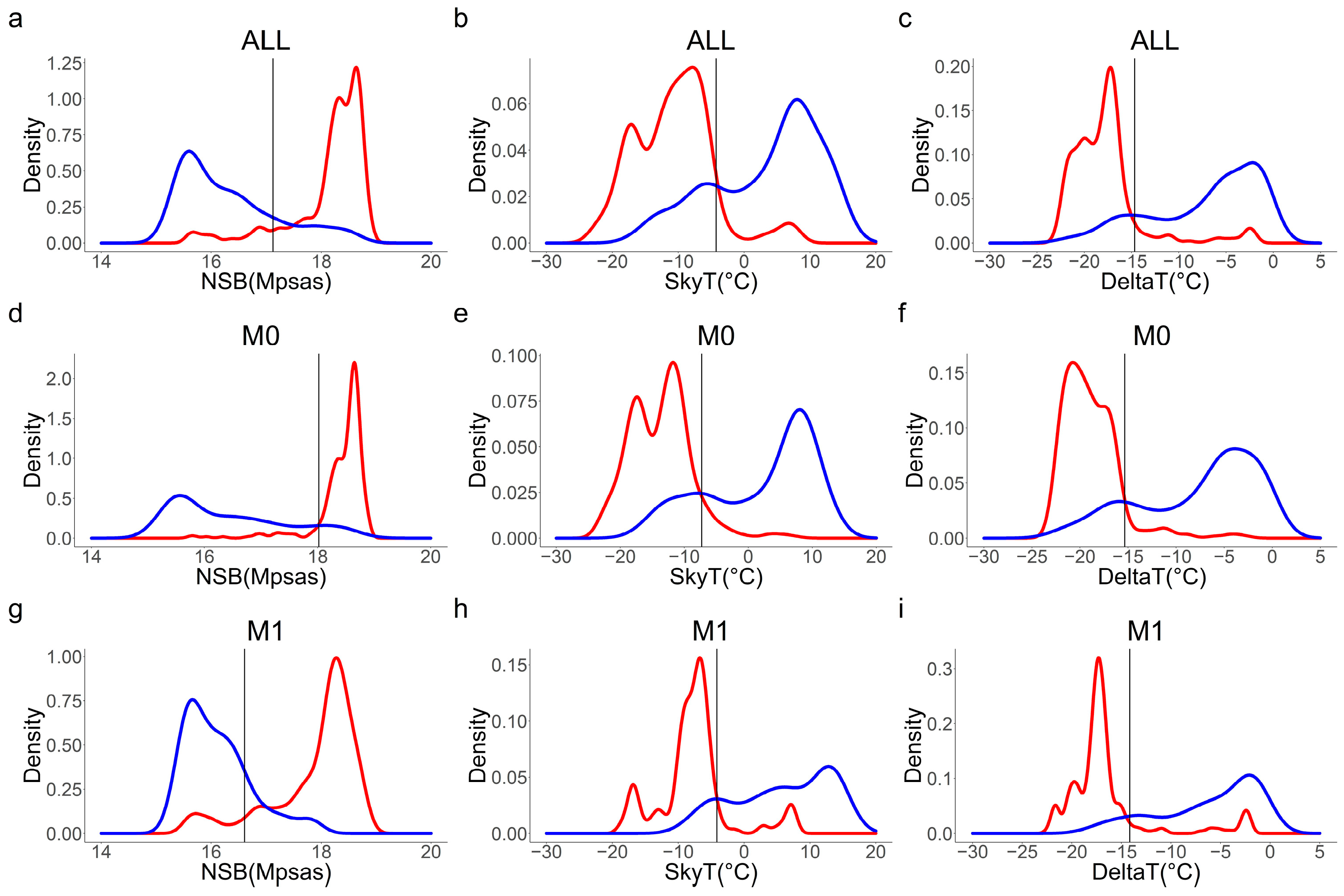
| M0C0 (Avg ± Sd) | M0C1 (Avg ± Sd) | M1C0 (Avg ± Sd) | M1C1 (Avg ± Sd) | |
|---|---|---|---|---|
| NSB (Mpsas) | 18.43 ± 0.45 ** | 16.44 ± 1.01 | 17.88 ± 0.79 ** | 16.13 ± 0.61 |
| SkyT (°C) | −13.75 ± 4.79 ** | 1.90 ± 8.36 | −7.68 ± 5.42 ** | 5.82 ± 7.18 |
| DeltaT (°C) | −18.88 ± 3.01 ** | −7.67 ± 6.06 | −16.55 ± 4.32 ** | −6.14 ± 5.00 |
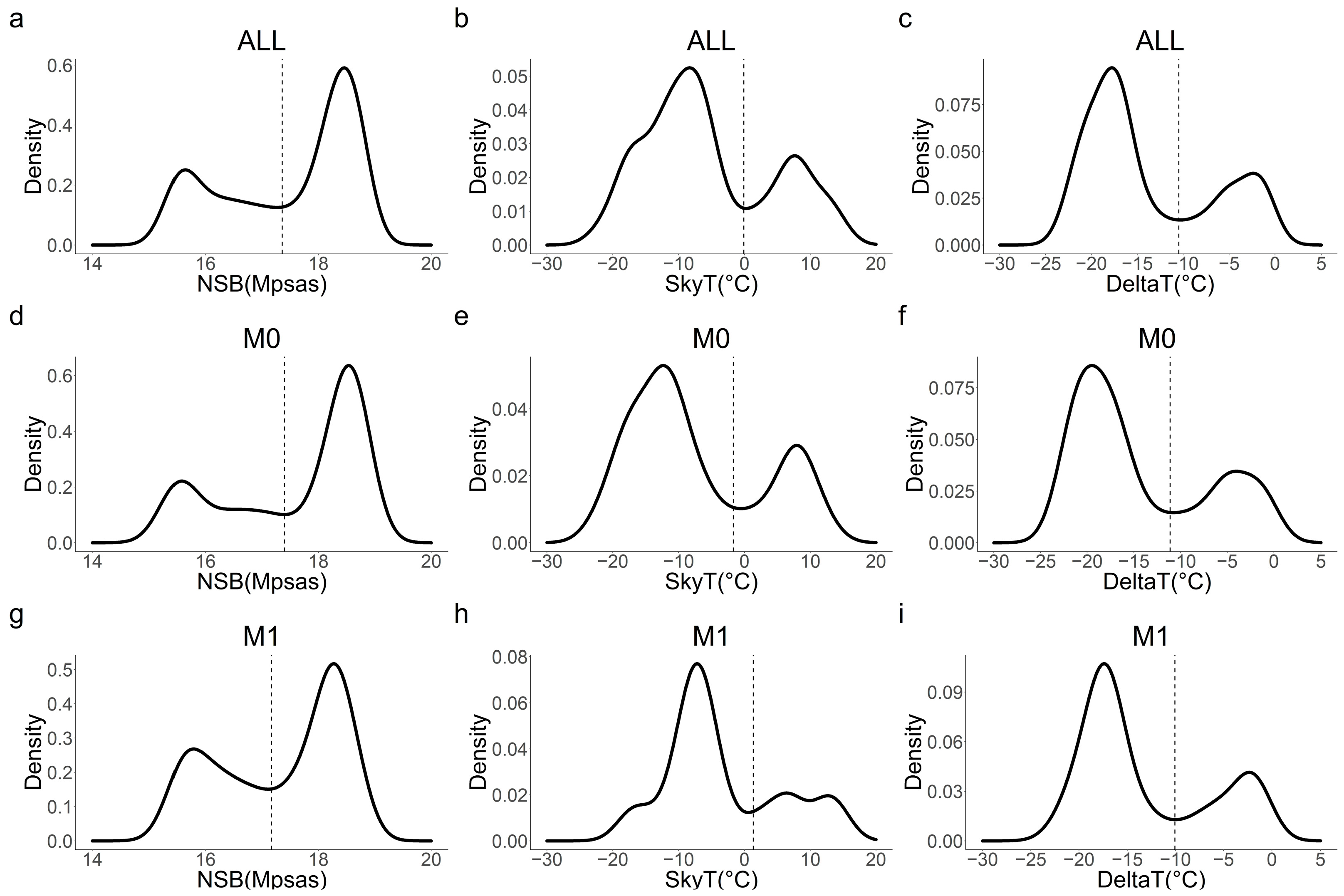
| Set | Parameter | Optimal Threshold | ACC | Antimode Threshold | ACC |
|---|---|---|---|---|---|
| ALL | NSB (MPSAS) | 17.12 | 0.87 | 17.36 | 0.87 |
| SkyT (°C) | −4.24 | 0.88 | −0.09 | 0.86 | |
| DeltaT (°C) | −14.67 | 0.89 | −10.48 | 0.87 | |
| M0 | NSB (MPSAS) | 18.02 | 0.91 | 17.4 | 0.89 |
| SkyT (°C) | −7.27 | 0.88 | −1.67 | 0.86 | |
| DeltaT (°C) | −15.34 | 0.89 | −11.11 | 0.87 | |
| M1 | NSB (MPSAS) | 16.61 | 0.89 | 17.17 | 0.86 |
| SkyT (°C) | −4.12 | 0.89 | 1.36 | 0.86 | |
| DeltaT (°C) | −14.16 | 0.90 | −10.05 | 0.87 |
Disclaimer/Publisher’s Note: The statements, opinions and data contained in all publications are solely those of the individual author(s) and contributor(s) and not of MDPI and/or the editor(s). MDPI and/or the editor(s) disclaim responsibility for any injury to people or property resulting from any ideas, methods, instructions or products referred to in the content. |
© 2023 by the authors. Licensee MDPI, Basel, Switzerland. This article is an open access article distributed under the terms and conditions of the Creative Commons Attribution (CC BY) license (https://creativecommons.org/licenses/by/4.0/).
Share and Cite
Massetti, L.; Materassi, A.; Sabatini, F. NSKY-CD: A System for Cloud Detection Based on Night Sky Brightness and Sky Temperature. Remote Sens. 2023, 15, 3063. https://doi.org/10.3390/rs15123063
Massetti L, Materassi A, Sabatini F. NSKY-CD: A System for Cloud Detection Based on Night Sky Brightness and Sky Temperature. Remote Sensing. 2023; 15(12):3063. https://doi.org/10.3390/rs15123063
Chicago/Turabian StyleMassetti, Luciano, Alessandro Materassi, and Francesco Sabatini. 2023. "NSKY-CD: A System for Cloud Detection Based on Night Sky Brightness and Sky Temperature" Remote Sensing 15, no. 12: 3063. https://doi.org/10.3390/rs15123063
APA StyleMassetti, L., Materassi, A., & Sabatini, F. (2023). NSKY-CD: A System for Cloud Detection Based on Night Sky Brightness and Sky Temperature. Remote Sensing, 15(12), 3063. https://doi.org/10.3390/rs15123063