Point2Tree(P2T)—Framework for Parameter Tuning of Semantic and Instance Segmentation Used with Mobile Laser Scanning Data in Coniferous Forest

Abstract

Inthis study, we introduce Point2Tree, a modular and versatile framework that employs a three-tiered methodology, inclusive of semantic segmentation, instance segmentation, and hyperparameter optimization analysis, designed to process laser point clouds in forestry. The semantic segmentation stage is built upon the Pointnet++ architecture and is primarily tasked with categorizing each point in the point cloud into meaningful groups or ’segments’, specifically in this context, differentiating between diverse tree parts, i.e., vegetation, stems, and coarse woody debris. The category for the ground is also provided. Semantic segmentation achieved an F1-score of 0.92, showing a high level of accuracy in classifying forest elements. In the instance segmentation stage, we further refine this process by identifying each tree as a unique entity. This process, which uses a graph-based approach, yielded an F1-score of approximately 0.6, signifying reasonable performance in delineating individual trees. The third stage involves a hyperparameter optimization analysis, conducted through a Bayesian strategy, which led to performance improvement of the overall framework by around four percentage points. Point2Tree was tested on two datasets, one from a managed boreal coniferous forest in Våler, Norway, with 16 plots chosen to cover a range of forest conditions. The modular design of the framework allows it to handle diverse pointcloud densities and types of terrestrial laser scanning data.

1. Introduction

The use of high-resolution 3D point clouds from terrestrial laser scanning (TLS), personalized laser scanning (PLS), and drone or helicopter-based laser scanning data has long been an area of intensive research for the characterization of forest ecosystems. In addition to measuring traditional variables such as stem volume, diameter, and height [1] or tree species (e.g., [2]), these very high-detail 3D forest structural data can allow new insights into single tree properties such as biomass (e.g., [3,4]), stem curves (e.g., [5]), tree height growth (e.g., [6]), wood quality (e.g., [7]), key ecological indicators [8], and phenotyping [9,10].

The emergence of improved sensor technology and the implementation of Simultaneous Localization And Mapping (SLAM) algorithms have greatly improved the availability and reduced the cost of dense point clouds from mobile laser scanning (MLS) platforms. The continuous move from stationary TLS to mobile, personalized, or drone-based scanning systems has greatly increased the ease of scanning larger forest plots [11]. Recent studies have also pointed out that personalized or mobile laser devices may provide an improved [12] or more cost-efficient [13] alternative to traditional field measurements with calipers and hypsometers for the collection of ground truth for air- or space-borne remote sensing.

At the core of most forest applications of high-density 3D point clouds is the ability to efficiently, with high precision and accuracy, segment the point cloud into different compartments such as stem, leaf, or branches (semantic segmentation) and further into single tree point clouds, hereafter referred to as instance segmentation. Even though the development of segmentation algorithms has been a substantial field of research for many years, both semantic and instance segmentation remains a significant bottleneck to unleashing the full potential of high-density point clouds in the forest context. Most studies have relied on algorithmic approaches (e.g., clustering and circle fitting or voxel-based approaches [14]) to identify and segment single trees [15,16]. In all cases, the segmentation routines tend to produce artifacts, and the single tree point clouds often require manual editing. In addition, such approaches are generally tailored to the specific data set and sensors they were developed on and are seldom transferable to new data.

Recent advances in the field of deep learning are triggering a new wave of studies looking into the possibilities to disentangle the complexity of high-density 3D point clouds and solve semantic [5,17], instance segmentation [18], and regression tasks [19]. One promising avenue in this field is the development of sensor-agnostic models that can learn general point cloud features and allow their transferability independently from the characteristics of the input point cloud. The advantage of such models is that they can be used off-the-shelf on new data without hyperparameter tuning. One exemplary case of moving in the direction of sensor-agnostic models for forest point clouds is the study by Krisanski et al. [17], who developed a semantic segmentation model to classify primary features (i.e., ground, wood, and leaf) in forest 3D scenes captured with TLS, ALS, and MLS. While desirable, there are currently no sensor-agnostic tree instance segmentation models for point cloud data. However, steps have been made to integrate sensor-agnostic deep learning semantic models with more traditional algorithmic pipelines to solve the instance segmentation challenge [17,19,20].

Wilkes et al. [21] addressed the instance segmentation problem in their tool TLS2Trees, which leverages on the FSCT semantic segmentation model published by Krisanski et al. [17]. In their approach, the wood-classified points from the semantic segmentation are used to construct a graph through the point cloud, then use the shortest path analysis to attribute points to individual stem bases. In the final step, the leaf-classified points are then added to each graph. A key aspect in this pipeline that affects the quality of the downstream products is the initial definition of the clusters performed using the DBSCAN clustering method [22]. The performance of DBSCAN depends on the separability of the instances, which is tightly linked to the output of the FSCT segmentation model (i.e., wood class parts, including stems, and branches) and to the forest type. In particular, instance clustering can be challenging in dense forests with a substantial amount of woody branches in the lower parts of the crown (e.g., Norway spruce forests). One potential avenue to boost the quality of the initial definition of the instances is to develop new point cloud semantic segmentation models that allow for a clearer separability of the instances by, for example, focusing on the main tree stem (i.e., excluding branches).

In TLS2Trees, the instance segmentation performance depends on a set of hyperparameters that should be individually tuned for a given type of forest to achieve the best possible performance. So far, both in TLS2Trees and other tree segmentation approaches tuning of these types of hyperparameters has traditionally been performed manually by individual researchers for each data set through trial and error processes. However, the possibility for a systematic and automated approach to hyperparameter optimization exists. Several potential methods that could solve the challenge exist (e.g., simulated annealing or Bayesian optimization [23]). Furthermore, it is also worth keeping in mind that the gradient-based methods may be ill-posed due to the non-convex profile of the hyperparameter space.

Gradient-based methods are powerful optimization algorithms that leverage the gradient of a function to find its minimum or maximum. These techniques are widely used in machine learning and deep learning, especially for training complex models such as neural networks. The general idea is to iteratively adjust the model’s parameters in the opposite direction of the gradient of the loss function (a measure of the model’s prediction error), aiming to reduce the loss [24]. Common examples include stochastic gradient descent (SGD) and its variants (e.g., Adam, RMSprop). Despite their efficiency, these methods have limitations when applied to non-convex optimization problems, such as hyperparameter tuning. Non-convex optimization landscapes can have many local minima, making it challenging for gradient-based methods to find the global minimum. Additionally, these methods require the computation of gradients, which may not always be possible or practical, especially when dealing with discrete hyperparameters or parameters that do not have values in all their spectrum (i.e., for some arguments function does not have value).

Leveraging on recent advances in semantic segmentation [17] and instance segmentation approaches [21], this study introduces Point2Tree which is a new modular framework for semantic and instance segmentation for MLS data. The Point2Tree has two main modules (1) a newly trained Pointnet++-based semantic segmentation model with the classes optimized for coniferous forest. 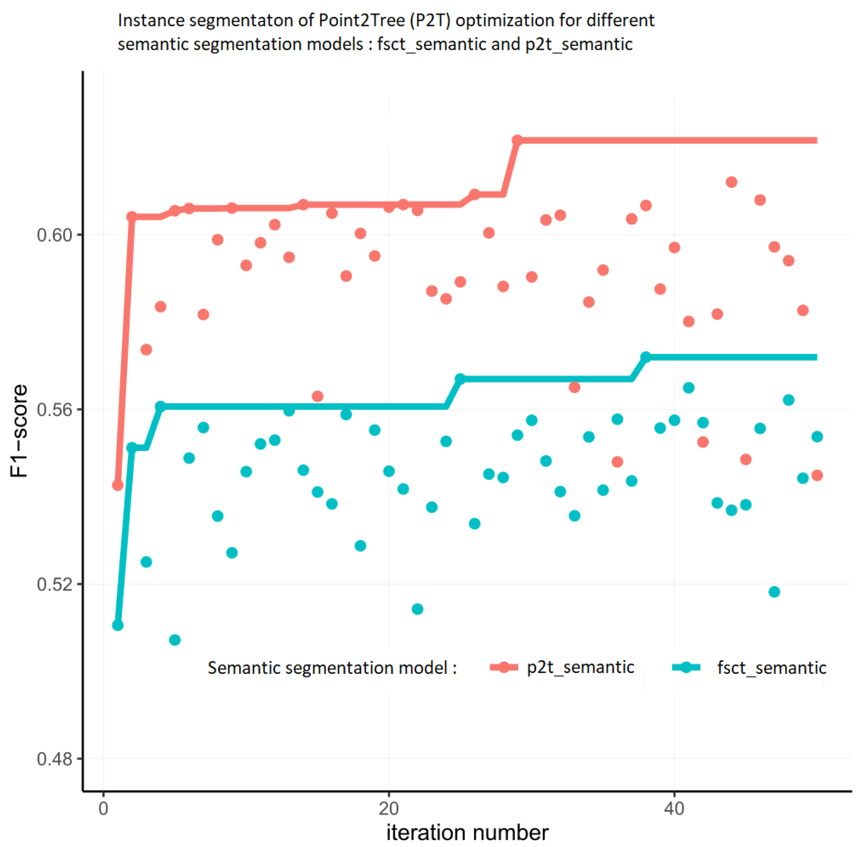), and (2) an optimization procedure for instance segmentation hyperparameter optimization based on the Bayesian flow approach [16]. Point2Tree is modular in the way that each of the components can be easily replaced by an improved module. We evaluate the performance of both the semantic and instance segmentation of Point2Tree with settings including: (a) with and without hyperparameter optimization and (b) with both the new semantic Pointnet++ model (i.e., p2t_semantic) as well as with the semantic model from FSCT [17], i.e., fsct_semantic. The evaluation is performed against a newly annotated dataset from our study area as well as an existing independent dataset from another part of Europe.

2. Materials

2.1. Study Area

The study area was located in an actively managed boreal coniferous dominated forest in Våler municipality in south-eastern Norway (N59.503219°, E10.884240°). A total of 16 circular plots of 400 ${\mathrm{m}}^2$ were purposefully selected to cover a range of forest conditions in terms of species composition (see Figure 1) and stand density (200–2500 trees ${\mathrm{h}\mathrm{a}}^{-1}$;

Table 1. Summary statistics for the selected plots.

	Min	Mean	Max	sd
trees ${\mathrm{h}\mathrm{a}}^{-1}$	200	1298	2500	638
dominant height [ $\mathrm{m}$]	15.6	22.4	29.0	4.1

). These plots included forests where the dominant species was either Norway spruce (Picea abies (L.) Karst.), Scots pine (Pinus sylvestris L.), or birch (Betula pubescens or Betula pendula), including different degrees of mixing between the species. Concerning the developmental stages, the selected plots were located either in mature forest stands or in stands in the middle of their rotation period. However, no young forests in the regeneration phase were included.

2.2. MLS Data Acquisition

Mobile laser scanning (MLS) data were collected in June 2022 using a GeoSLAM ZEB-HORIZON [25] in correspondence with the 16 circular field plots of 400 ${\mathrm{m}}^2$ area. The data collection was initialized by booting the GeoSLAM ZEB-HORIZON in the center of the field plot. Consequently, the operator walked: (i) two perpendicular eight figures, centered in the plot center and extending to a maximum distance of 15 $\mathrm{m}$ from the center, and (ii) a circumference corresponding to the plot perimeter (radius of 15 $\mathrm{m}$). The data collection lasted for 10–15 $\min$ per plot. The raw MLS data were then processed within the GeoSLAM Hub software relying on a proprietary SLAM algorithm. The resulting point clouds were down-sampled to only 9% of the total points and exported as .las files. This value is the default value in GeoSLAM Hub software, which in previous experiences was found to reduce data redundancy while maintaining the 3D structure information. The whole point clouds were further clipped to include only the area of the plot plus a buffer of 5 $\mathrm{m}$ around the plot area to ensure that all crowns of trees at the edge of the plots could be segmented.

2.3. Point Cloud Annotation

The point clouds corresponding to the 16 selected plots were manually annotated using CloudCompare [26] by a team of two annotators, followed by a review step by the annotators’ administrator. The annotation consisted of two consecutive steps: (1) Instance annotation: segmentation of single trees if they could be identified as trees (i.e., not always possible for small understory trees). The segmentation was performed so that branches of intermingled trees were separated as far as practically possible. (2) Semantic annotation: the annotators classified every single point into the following classes: ground, vegetation (branches, leaves, and low vegetation), coarse woody debris (i.e., deadwood), and stems. The classes were the same as those defined by Krisanski et al. [17], with the difference that the stems were separated from the branches and assigned to a general vegetation class. The reason behind this modification of the semantic classes was that the stems are distinct features in coniferous forests that can enable a more precise separation of the single instances. The points from trees with the stem at breast height outside the plot were removed from further analysis. The visualization of the annotation process was presented in Figure 2.

We followed the same split approach by Krisanski et al. [17] and divided the circular plot into four radial slices and randomly assigned two for training (50%), one for validation (25%) and one for the testing (25%). A complete overview of the segmented plot can be found in the Appendix A in Figure A1.

3. Methods

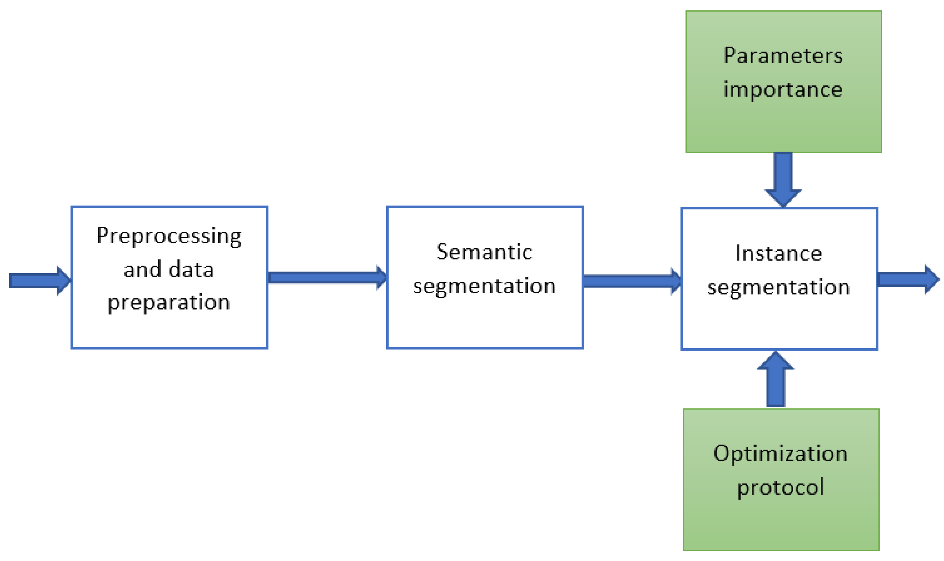
The pipeline used in this work comprises several stages, as presented in Figure 3 and Figure 4. It is worth noting that due to the large size of point cloud files, arranging all the steps in the pipeline well and orchestrating their behavior to obtain a good system performance is essential. In some cases, it may be hard to arrive at the processing results due to ineffective data processing which does not account for all the aspects of the data well. This effect may mostly occur when dealing with locally very sparse point clouds (often on borders of the cloud). Therefore, all steps are prepared in a modular fashion and the stages are parameterized so they can be adjusted to different densities and types of point clouds. Furthermore, the steps of the pipeline are prepared in a way that enables smooth substitution of selected components of the system. The elements of the system are interconnected using a programming language agnostic composition strategy as presented in Figure 3.

Within this work, we used a custom naming convention.

Table 2. Components of the pipeline and their properties. * This is fsct_semantic but trained on our data.

Components of the Pipeline	FSCT [17]	TLS2trees [21]	Point2Tree (P2T)
Semantic seg.	fsct_semantic	tls_semantic	p2t_semantic *
Instance seg.	fsct_instance	tls_instance	tls_instance
Optimization	no	no	yes
Analytics	no	no	yes
Language agnostic modularity	no	no	yes

presents a set of acronyms and features of different pipelines we partially based our framework on and which we compare against our performance. Point2Tree framework is equipped with optimization, and analytics modules and also enables the incorporation of external modules implemented in different programming languages thanks to its modular architecture. This feature of P2T was used in order to employ semantic segmentation from FSCT and instance segmentation from TLS pipelines.

It is worth noting that “p2t_semantic” was obtained from “fsct_semantic” by replacing the original set of FSCT weights of the Pointnet++ model with the model trained on our data.

3.1. Data Preprocessing

In the preprocessing step, the initial tiling operation is performed. Tile size is adjustable and should be chosen based on the data profile. It is also worth noting that there is usually an entire range of low-density point cloud tiles at the edges of point clouds. These data are difficult to digest for both semantic segmentation and instance extraction part of the pipeline. Therefore, a dedicated procedure to remove these low-density tiles was adopted. The procedure examines all the tiles in terms of their point density. A tile is removed from further processing if the density is below a critical threshold. As may be noticed, the tiles’ granularity strictly affects the point cloud’s shape after the protocol. The effect of the density-based tiling protocol is presented in Figure 4.

3.2. Semantic Segmentation

In our workflow, Pointnet++ [17,27] implemented in Pytorch was used as a base model for semantic segmentation. The model was trained from scratch using the newly annotated dataset (p2t_semantic, see Table 2).

The point cloud was sliced into cube-shaped regions to prepare the data for Pointnet++. Each cube was shifted to the origin before inference to avoid floating-point precision issues. The preprocessing is performed before training or inference, and each sample is stored in a file to minimize computational time and facilitate taking advantage of parallel processing. The preprocessing also takes advantage of vectorization by using the NumPy package.

During training, we used subsampling and voxelization protocol to 1 $\mathrm{cm}$. The parameters used in the training process are listed in

Table 3. The parameters used in the training process for p2t_semantic module.

Parameter Name	Value
$\mathrm{num}\text{\_}\mathrm{epochs}$	300
$\mathrm{learning}\text{\_}\mathrm{rate}$	$0.00005$
$\mathrm{input}\text{\_}\mathrm{point}\text{\_}\mathrm{cloud}$	$\mathrm{None}$
$\mathrm{sample}\text{\_}\mathrm{box}\text{\_}\mathrm{size}\text{\_}\mathrm{m}$	$[6,6,8]$
$\mathrm{sample}\text{\_}\mathrm{box}\text{\_}\mathrm{overlap}$	$[0.5,0.5,0.5]$
$\min \text{\_}\mathrm{points}\text{\_}\mathrm{per}\text{\_}\mathrm{box}$	1000
$\max \text{\_}\mathrm{points}\text{\_}\mathrm{per}\text{\_}\mathrm{box}$	$20,000$
$\mathrm{subsample}$	$\mathrm{True}$
$\mathrm{subsampling}\text{\_}\min \text{\_}\mathrm{spacing}$	$0.01$

, and the training was performed on Nvidia GV100GL [Tesla V100S PCIe 32GB].

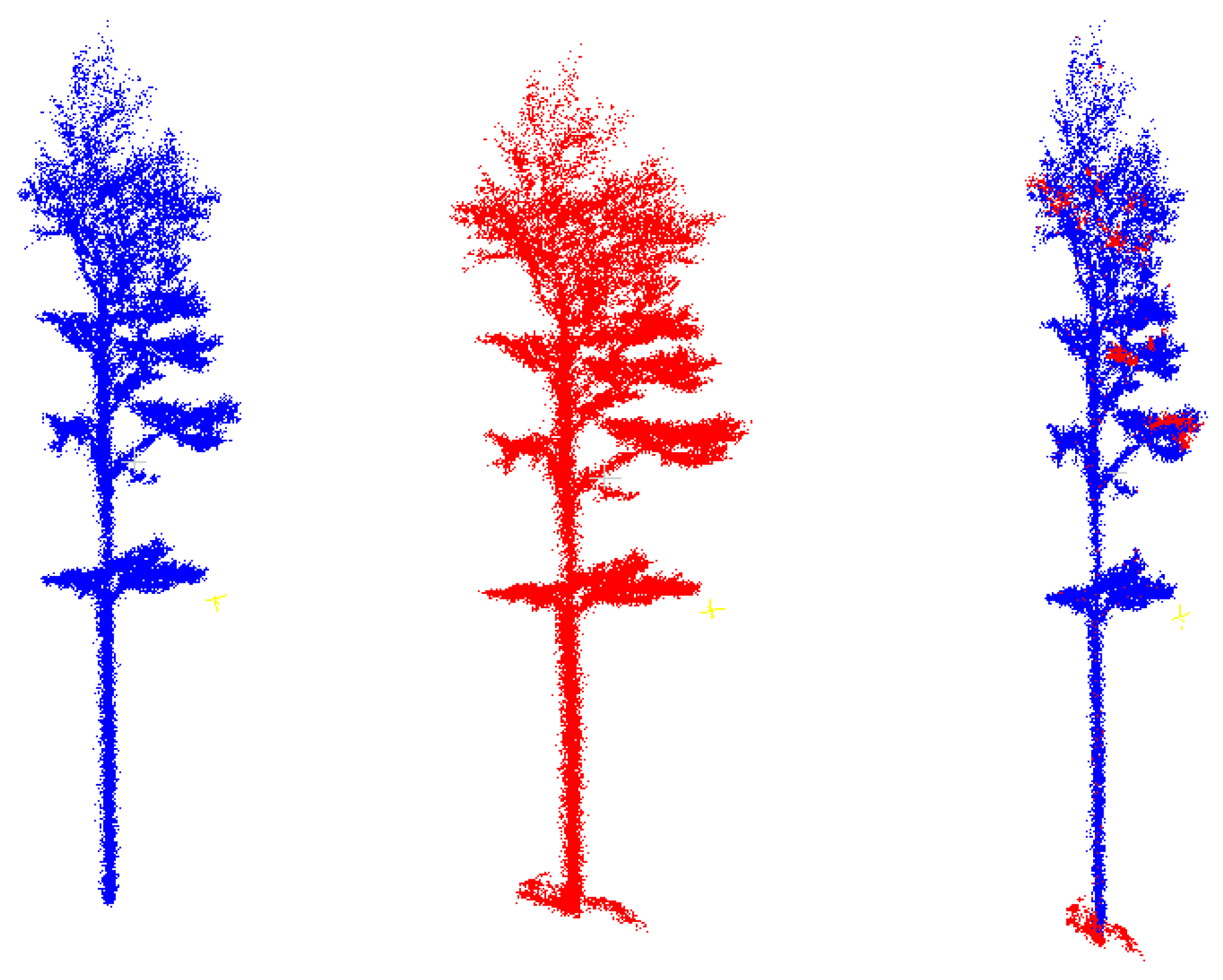
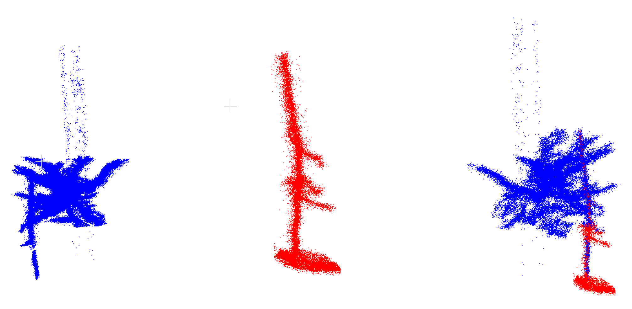
3.3. Instance Segmentation

We employed the TLS2trees instance segmentation technique [21]. This method separates the individual tree through a series of steps, including: (i) initial semantic segmentation as input; (ii) tree-wise graph construction using the wood (i.e., or stem based on our proposed semantics) classified points; and (iii) addition of the leaves (or crown) by extending the tree-wise graphs to the rest of the tree crown. A comprehensive explanation of this approach is provided in [21]. It is important to note that the accuracy of the instance segmentation is strongly affected by the results of the semantic segmentation as well as the quality of the data employed for training this model.

3.4. Evaluation

Evaluating machine learning models and pipelines can be challenging, as it requires providing an appropriate set of metrics and a protocol for applying them in a repeatable and reliable way. While it is much easier to develop a protocol if the point matching at the cloud level is ensured, there is still a way to compare results against the ground truth when that is not the case.

In the solution presented in this paper, the input data is down-sampled during the pre-processing, leaving only a single random point per voxel. As a result, the number of output points is lower than the input points. There are also small distortions introduced related to several point-cloud conversions in the process of mapping between data formats. We provide a method based on the KNN algorithm for point matching. Our method consists of the following steps:

• An algorithm for iterative tree elimination:

  (a)

  Find the biggest trees in the GT.

  (b)

  Find the biggest overlap in PD.

  (c)

  Assign GT (Ground Truth) to PD (predicted) and eliminate PD.

  (d)

  Add to collection (dictionary).

• Compute tree-level metrics based on the dictionary.

We aggregate results on multiple levels and use a set of common metrics such as the F1-score and IOU (Jaccard index) to assess the performance of the model on a pixel level.

$$\mathrm{Precision}=\frac{\mathrm{True}\mathrm{Positives}\left(\mathrm{TP}\right)}{\mathrm{True}\mathrm{Positives}\left(\mathrm{TP}\right)+\mathrm{False}\mathrm{Positives}\left(\mathrm{FP}\right)}$$

(1)

$$\mathrm{Recall}=\frac{\mathrm{True}\mathrm{Positives}\left(\mathrm{TP}\right)}{\mathrm{True}\mathrm{Positives}\left(\mathrm{TP}\right)+\mathrm{False}\mathrm{Negatives}\left(\mathrm{FN}\right)}$$

(2)

$$\mathrm{F}1\mathrm{Score}=2·\frac{\mathrm{Precision}·\mathrm{Recall}}{\mathrm{Precision}+\mathrm{Recall}}$$

(3)

$$\mathrm{IoU}(\mathrm{Jaccard}\mathrm{index})=\frac{\mathrm{Area}\mathrm{of}\mathrm{Overlap}}{\mathrm{Area}\mathrm{of}\mathrm{Union}}$$

(4)

Also, the residual height operating on a tree level (Equation (5)) as the difference between ground truth height (gt) and predicted height (pred) of trees is calculated.

$$h_{\mathrm{res}}=h_{\mathrm{gt}}-h_{\mathrm{pred}}$$

(5)

The square root of the average squared difference between ground truth heights (h_gt) and predicted heights (h_pred) over a dataset is given by Equation (6)

$$\mathrm{RMSE}=\sqrt{\frac{1}{N}{\displaystyle \sum _{i=1}^N}{(h_{{\mathrm{gt}}_i}-h_{{\mathrm{pred}}_i})}^2}$$

(6)

For large datasets, serial execution of the metrics is pretty slow; thus, a parallel version was implemented and used for experiments in this work.

3.5. Optimization

This work proposes an optimization protocol based on a Bayesian approach [23,28,29]. It is a sequential method that gradually explores the space of hyperparameters, focusing on the most promising manifolds within it. This method is especially suitable for applications where each iteration is time-consuming, as is the case with processing a large volume of point cloud data, presented in this work. In particular, we compute the F1-score (Equation (3)) as a function of point cloud instance segmentation.

The method works by constructing a probabilistic model, typically a Gaussian Process (GP), to represent the unknown function and then using an acquisition function to balance exploration and exploitation when deciding on the next point to sample. The objective is to find the global optimum with as few evaluations as possible. The GP is defined by a mean function $\mu \left(\mathrm{x}\right)$ and a covariance function $k(\mathrm{x},{\mathrm{x}}^{\prime })$, which together describe the function’s behavior. The choice of kernel function is crucial for the performance of Bayesian optimization as it encodes the prior belief about the function’s smoothness. A commonly used kernel is the squared exponential kernel:

$$k(\mathrm{x},{\mathrm{x}}^{\prime })={\sigma }_f^{2}exp\left(-\frac{{(\mathrm{x}-{\mathrm{x}}^{\prime })}^2}{2l^2}\right)$$

(7)

where ${\sigma }_f^2$ represents the signal variance and l is the length scale parameter, $\mathrm{x},{\mathrm{x}}^{\prime }$ are input vectors for which we want to compute the covariance. They are multi-dimensional and model tree hyperparameters setup.

In the Bayesian optimization framework, we start with a prior distribution over the unknown function, and after each evaluation, we update our beliefs using Bayes’ rule. This results in a posterior distribution, which is used to guide the search for the global optimum [23].

The instance segmentation stage is composed of multiple modules that contain a series of hyperparameters that should be optimized to reach the best possible performance of the model. The most important ones are depicted in Figure 5, and tested values are shown in

Table 4. Optimization parameters and their ranges. See Figure 5 and [21] for parameter definitions.

Parameter	Values
$\mathrm{slice}\text{\_}\mathrm{thickness}$	$[0.25,0.5,0.75]$
$\mathrm{find}\text{\_}\mathrm{stems}\text{\_}\mathrm{height}$	$[0.5,0.75,1.0,1.5,2.0]$
$\mathrm{find}\text{\_}\mathrm{stems}\text{\_}\mathrm{thickness}$	$[0.25,0.5,0.75]$
$\mathrm{graph}\text{\_}\mathrm{maximum}\text{\_}\mathrm{cumulative}\text{\_}\mathrm{gap}$	$[1,2,3,4]$
$\mathrm{add}\text{\_}\mathrm{leaves}\text{\_}\mathrm{voxel}\text{\_}\mathrm{length}$	$[0.25,0.5,0.75]$
$\mathrm{find}\text{\_}\mathrm{stems}\text{\_}\min \text{\_}\mathrm{points}$	$[10,20,30,50,100,150,200]$

.

The chosen values of the hyperparameters cover the most promising and useful ranges. It is worth noting that the choice and the number of parameters affect the performance of the optimization algorithm. Consequently, they should be picked according to the specific profile of the forest dataset in question.

The optimization process of Point2Tree involves many iterations of the pipeline execution with a distinct set of parameters. Therefore, applying a well-structured protocol to address this process is reasonable.

In each iteration of the optimization process, the F1-score is derived from the complete dataset, and the algorithm maximizes its value over the steps of the execution.

The optimization is performed by optimizing the F1-score for the entire set. The overall F1-score is calculated using a three-fold protocol as given by Algorithm 1.

Algorithm 1 F1-score calculation

1: for plot in dataset do 2:   for for tree in plot do 3:     Compute F1-score 4:   end for 5:   Aggregate F1-score per plot 6: end for 7: Aggregate F1-score per dataset

Based on the F1-score the optimization algorithm guides the next steps of the optimization. In our research and experiments, we noticed that it is possible to improve the optimization results by decomposing the process into several stages. After the initial stage (e.g., 40 runs), it is possible to stop the optimization and restart it for a limited and the most important set of parameters. Sample implementation of this approach is given by Algorithm 2.

Algorithm 2 Optimization Algorithm—two-stage protocol

Require: Initial parameters   1: Run initial optimization   2: Select less than four parameters of the highest importance   3: Run optimization for the selected parameters Ensure: Optimized parameters

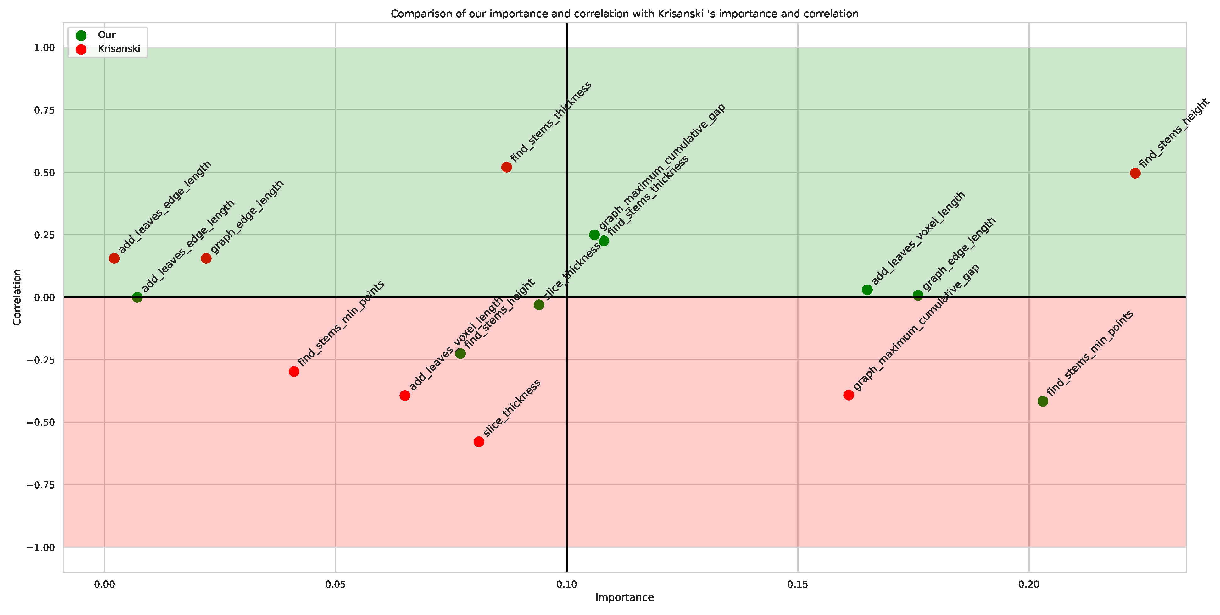
Point2Tree provides a module for assessing the importance of hyperparameters in the optimization process. The results are presented in the Appendix A.

3.6. Final Validation

After completing the optimization, we evaluated the best set of hyperparameters for both Point2Tree (P2T) with fsct_semantic and p2t_semantic. To validate our results, we compared them against the LAUTx dataset, a benchmark for the instance segmentation [30].

Aside from the F1-score, we evaluated additional metrics, including precision, recall, residual height, detection, commission, and omission rate. Finally, we provided comparisons for the regular model with standard parameters used in [21] and the optimized set of parameters.

4. Results and Discussion

4.1. Semantic Segmentation Performance

The newly trained p2t_semantic model achieved precision, recall, and an F1-scores of 0.92. The F1-score ranking per class (vegetation, terrain, and stem) reflected the proportions of these classes in the training data, as shown in

Table 5. Number of point-cloud points in the dataset used for training semantic segmentation model p2t_semantic.

Class	Count	Percentage (%)
Terrain	16,460,251	24.94
Vegetation	40,332,257	61.12
CWD	225,093	0.34
Stem	8,972,140	13.60

. Vegetation was the most common class, representing over 61% of the dataset, while CWD and stem were the least common, accounting for only 0.34% and 13.6% of the dataset, respectively. The confusion matrix for p2t_semantic model is shown in Figure 6, while

Table 6. Class-wise metrics for p2t_semantic semantic segmentation.

	Class
Metric	Terrain	Vegetation	Stem
Precision	0.86	0.94	0.94
Recall	0.93	0.92	0.82
F1-score	0.89	0.93	0.87

shows the class-wise metrics for semantic segmentation.

4.2. Instance Segmentation Optimization

We applied the Bayesian flow for the optimization of hyperparameters for the instance segmentation [23] and considered all the hyperparameters as presented in Table 4. We optimized the hyperparameters for (1) TLS2Trees [21] that uses the semantic segmentation from FCST, i.e., fsct_semantic [17] and (2) Point2Tree, which uses the semantic segmentation model developed in this paper and the instance segmentation framework from TLS2Trees, i.e., tls_instance.

The optimization was interrupted after 50 iterations as only minor marginal improvements were observed for both tested models (see Figure 7). Interestingly, when considering all iterations, the rate of growth of the F1-score over the number of iterations was negative for the optimization of Point2Tree (slope of −0.0002). At the same time, it was slightly positive TLS2Trees (slope of 0.0002). These numbers indicate that the method Point2Tree was more robust to variations in the choice of hyperparameters. Such property is desired and might be explained by the definition of the instances being more robust when based only on clean stems rather than using a class merging stems and woody branches.

The analysis of the importance of the different hyperparameters on the F1-score revealed differences between the two approaches. In particular, we found the following for the respective hyperparameters:

• $\mathrm{find}\text{\_}\mathrm{stem}\text{\_}\mathrm{height}$: there was a contrasting effect between the Point2Tree with p2t_semantic and fsct_semantic. In the latter, $\mathrm{find}\text{\_}\mathrm{stem}\text{\_}\mathrm{height}$ was the important hyperparameter, while it was the least important for the p2t_semantic approach. Point2Tree results showed that the fsct_semantic segmentation approach selected higher (approx. 1.75 m above ground) slices, whereas p2t_semantic preferred close-to-the-ground (approx. 0.8 m) slices. The need for fsct_semantic to search for tree instances higher up the stem might be due to larger noise due to low branches and low vegetation in the wood instance class used for clustering the instances. In this context, p2t_semantic proved more robust in filtering out low-vegetation and non-stem points.
• $\mathrm{find}\text{\_}\mathrm{stems}\text{\_}\mathrm{thickness}$: for this hyperparameter, defining the thickness of the slice used for clustering the instances, the two approaches also behaved differently, with P2T-fsct_semantic approach tended to select narrower (approx. 20 cm) slices, whereas P2T with p2t_semantic approach preferred wider (approx. 0.75 m) slices. The selection of narrower search windows in the P2T-fsct_semantic approach, coupled with the selection of higher slices, is needed to reduce the noise due to branches and low vegetation. Using wider slices allows for including more extensive portions of a tree stem, thus increasing the chance of detecting single instances.
• $\mathrm{find}\text{\_}\mathrm{stem}\text{\_}\min \text{\_}\mathrm{points}$: this was the most crucial hyperparameter for the P2T-p2t_semantic approach and was negatively correlated with the F1-score (−0.4), meaning that the minimum number of points to trigger a new instance was 50–100 points, rather than 200 points in the P2T-fsct_semantic default values. On the other hand, for the P2T-fsct_semantic approach, this hyperparameter was the second least important and negatively correlated with the f1-score(−0.26), preferring values between 100 and 120 points.
• $\mathrm{graph}\text{\_}\mathrm{edge}\text{\_}\mathrm{length}$: This was the second most important hyperparameter for the P2T-p2t_semantic approach but was very weakly correlated (0.008) with the F1-score. The preferred value for the P2T-pt2_semantic model was around 1 m, the same as the default value in TLS2trees. For the P2T-fsct_semantic approach, the most suitable values were in the 0.4–0.6 m range. This is the maximum length an edge in the graph can be. If this is set to a larger value then disconnected points (occlusion) can be connected although this may bridge gaps between trees. It relates to the flexibility of the graph growth, and the P2T-fsct_semantic approach is more rigid.
• $\mathrm{graph}\text{\_}\mathrm{maximum}\text{\_}\mathrm{cumulative}\text{\_}\mathrm{gap}$: We can see that (Figure 8) this hyperparameter has a contrast effect on P2T-p2t_semantic and P2T-fsct_semantic approaches. In the P2T-pt2_semantic approach, it has a pretty high positive correlation (0.25) and kind of medium importance, which means that long gaps are accepted, resulting in more additional stems and branches to be included (see [21] Figure 7). This is acceptable and desirable in the P2T-p2t_semantic case since we skip branches and focus only on trunks. In the P2T-fsct_semantic method, the smaller values of $\mathrm{graph}\text{\_}\mathrm{maximum}\text{\_}\mathrm{cumulative}\text{\_}\mathrm{gap}$ are preferred, which may be considered an attempt to reduce the noise in the form of small branches and stems. The parameter is also important in P2T-fsct_semantic.
• $\mathrm{add}\text{\_}\mathrm{leaves}\text{\_}\mathrm{voxel}\text{\_}\mathrm{length}$: In the case of the P2T-p2t_semantic approach, the parameter is quite important (approx. 016) and slightly positively correlated. Those values indicate that the voxel size affects the output F1-score of our method. This relation is expected because our method is based on trunk modeling without branches, so the size of the leaf voxel is important. On the other hand, attempting to manipulate this parameter does not lead to high gains in model performance. Conversely, this parameter has a negative (approx. −0.35) correlation in the P2T-fsct_semantic method but even smaller importance. This lack of impact can be explained by the fact that since the P2T-fsct_semantic approach is based on the branches, the size of the leaf voxels is not that critical, and also, it is preferred to be low to give more freedom to the graph constructing algorithm in TLS.
• $\mathrm{add}\text{\_}\mathrm{leaves}\text{\_}\mathrm{edge}\text{\_}\mathrm{length}$: This parameter, in both the approaches, has a low correlation and low importance. The overall impact of the parameter on the output is relatively low.
• $\mathrm{slice}\text{\_}\mathrm{thickness}$: This parameter is unimportant in both methods. However, it is worth noting that in the case of the P2T-fsct_semantic method, it has a more negative correlation. Therefore, in the P2T-fsct_semantic approach, it is better to have smaller slices, which can be beneficial since the algorithm operates on branches. On the other hand, in the P2T-p2t_semantic approach, trunks are more distinguishable as an effect of the lack of branches, so the TLS algorithm can allow larger slices, which is reflected in the correlation of the parameter.

A more detailed examination of Figure 8 reveals two P2T-fsct_semantic and five P2T-p2t_semantic hyperparameters in the right part of the plot. It means that for the P2T-fsct_semantic approach, there are two important and contrasting parameters, namely $\mathrm{graph}\text{\_}\mathrm{maximum}\text{\_}\mathrm{cumulative}\text{\_}\mathrm{gap}$ and $\mathrm{find}\text{\_}\mathrm{stem}\text{\_}\mathrm{height}$; whereas, for the P2T-p2t_semantic method, there are five of them. Furthermore, in the case of the P2T-p2t_semantic approach, the optimization landscape is blurry since we need to manipulate five fewer contrasting parameters.

4.3. Metrics Evaluation

4.3.1. On Test Data from This Study

The evaluation of the metrics computed against the test data (see

Table 7. Instance segmentation results on the test dataset.

Evaluation Metric	P2T-p2t_semantic	Optimized P2T-p2t_semantic	P2T-fsct_semantic	Optimized P2T-fsct_semantic
Precision	0.6	0.65	0.57	0.678
Recall	0.61	0.65	0.57	0.644
F1-score	0.57	0.61	0.54	0.625
Intersection over Union (IoU)	0.47	0.5	0.45	0.514
Residual Height (gt—pred) [m]		0.87		0.907
Root Mean Square Error (RMSE) of Height Errors [m]		3.47		3.597
True Positive (detection rate)		0.57		0.594
False Positive (commission)		0.36		0.262
False Negative (omissions)		0.07		0.144

) revealed that using optimal parameters resulted in a performance boost compared to using default values for both P2T with p2t_semantic and fsct_semantic. In line with the optimization findings, the magnitude of the improved performance for P2T-fsct_semantic was twice as large (0.08 F1-score increase) compared to P2T-p2t_semantic (0.04 F1-score increase). When optimized, both approaches reached similar levels of F1-score. Despite the marginal differences, P2T with p2t_semantic approach resulted in a smaller residual height of 0.87 m and 3.47 RMSE and a lower detection rate than P2T-fsct_semantic. The analysis of the false positive rates indicated that both approaches tended to over-segment the point clouds, and such behavior was more prominent in P2T-p2t_semantic. On the other hand, it is essential to highlight that while having more significant commission errors, the P2T-p2t_semantic model reduced the false negatives (i.e., omitted trees) to nearly zero.

The experiments presented in Table 7 were conducted for a set of the best hyperparameters which we obtained in the optimization process. The set is given in

Table 8. Set of the best parameters for both models.

Parameter	P2T-fsct_semantic	P2T-p2t_semantic
$\mathrm{add}\text{\_}\mathrm{leaves}\text{\_}\mathrm{edge}\text{\_}\mathrm{length}$	1.115	0.991
$\mathrm{add}\text{\_}\mathrm{leaves}\text{\_}\mathrm{voxel}\text{\_}\mathrm{length}$	0.159	0.317
$\mathrm{find}\text{\_}\mathrm{stems}\text{\_}\mathrm{height}$	1.614	0.797
$\mathrm{find}\text{\_}\mathrm{stems}\text{\_}\min \text{\_}\mathrm{points}$	84	105
$\mathrm{find}\text{\_}\mathrm{stems}\text{\_}\mathrm{thickness}$	0.46	0.75
$\mathrm{graph}\text{\_}\mathrm{edge}\text{\_}\mathrm{length}$	0.66	1.086
$\mathrm{graph}\text{\_}\mathrm{maximum}\text{\_}\mathrm{cumulative}\text{\_}\mathrm{gap}$	6.826	14.845
$\mathrm{slice}\text{\_}\mathrm{thickness}$	0.678	0.833

.

4.3.2. On the LAUTx Data

The results from applying the P2T with fsct_semantic and P2T with p2t_semantic pipelines to the LAUTx data for each of the different sets of hyperparameters revealed that both approaches performed consistently or even better than what was found for our initial test data (see

Table 9. Instance segmentation benchmark LAUTx dataset [30].

	P2T with p2t_semantic		P2T with fsct_semantic
Metric	Default	Optimized	Default	Optimized
Precision	0.826	0.787	0.773	0.771
Recall	0.588	0.528	0.57	0.506
F1-score	0.669	0.603	0.629	0.578
Intersection over Union (IoU)	0.533	0.461	0.502	0.442
Residual Height (gt—pred) [m]	0.484	0.563	0.967	1.094
Root Mean Square Error (RMSE) of Height Errors [m]	2.66	3.496	3.589	4.971
True Positive (detection rate)	0.552	0.422	0.405	0.366
False Positive (commission)	0.294	0.456	0.29	0.427
False Negative (omissions)	0.154	0.122	0.304	0.207

).

Interestingly, the default parameters were more suitable than the optimized hyperparameters, highlighting the need for more extensive and varied datasets of annotated plots for more robust optimization. Alternatively, the optimization process can be performed separately for each dataset but this requires that a part of a dataset is labeled for the Point2Tree pipeline for adjusting the hyperparameters of the instance segmentation.

The P2T with p2t_semantic approach performs slightly better than the P2T fsct_semantic. This result may stem from the p2t_semantic model focusing more on the trunks, and the LAUTx dataset [30] is composed of high and mostly separated trees.

Sample results of the performance of the P2T-p2t_semantic on the LAUTx dataset [30] are provided in Figure 9.

In order to visualize the performance of the metrics used in the experiments, we have provided a series of plots for different quality of results. They are given by Figure 10, Figure 11 and Figure 12. We can see that the number of artifacts grows once the metrics values go down. It is also worth noting that some artifacts are specific to a given dataset labeling process. For instance, as we can see in Figure 10, Figure 11 and Figure 12, the bottom of tree trunks were very deeply labeled, such that the labeling account for a part of the ground. This issue is not the case for the data p2t_semantic model was trained on. Thus, it is hard to achieve a perfect metric on the LAUTx dataset [30].

5. Conclusions

This study presents a new framework for point cloud instance segmentation. The framework consists of a series of components that are structured in a flexible way. This allows us to replace selected parts of the pipeline (e.g., instance segmentation) with new or alternative modules. The new modules may be implemented in alternative languages (e.g., C++, java, etc.) and the integration is still possible. The framework is also equipped with an optimization module and insightful parameters visualization.

We also tested the effect of hyperparameter tuning on the TLS2trees instance segmentation pipeline, developed initially for tropical forests, to optimal settings for coniferous forests. Further, we tested the effect of using a semantic segmentation model specifically designed to focus on identifying the stems of coniferous trees on the tree instance segmentation accuracy. Our study found that the hyperparameter tuning positively affected the segmentation output quality of our data. However, when applying the same parameters to the external LAUTx dataset, the performance was poorer than using the default setting. This result indicates that to estimate a more robust and transferable set of hyperparameters, we need to develop more extensive databases of openly available annotated point cloud data spanning a broader range of forest types than those used in this study. When optimized, the effect of using different semantic segmentation models (i.e., P2T with p2t_semantic and fsct_semantic) was marginal. However, it is also true that the instance segmentation relying on the p2t_semantic model seemed less sensitive to the choice of hyperparameters and thus more robust in dense forests or forests with many low branches (e.g., non-self-pruning species). Due to the architecture of the instance segmentation algorithm, there were certain combinations of hyperparameters that led to the failure of execution of the pipeline, thus imposing a constraint in the choice of the protocol for hyperparameter tuning, i.e., the Bayesian approach for which the space of the hyperparameters does not have to be convex.

Overall the performance of the Point2Tree was high, and the approach holds significant promise toward automated semantic and instance segmentation of 3D point clouds. At the same time, the results illustrate several avenues for further improvement and development: (1) training the algorithms on larger sets of data from a broader range of forest types is an obvious avenue for potential improvement, (2) the semantic component of Point2Tree is a deep-learning-based approach while the instance segmentation relies on a more algorithmic (graph-based) approach that relies on a good representation of the individual stems in the point clouds. Replacing the algorithmic component of Point2Tree with a deep-learning-based approach, like segmentation, may be beneficial in terms of computational demands for deployment and less reliance on a good representation of the stem in the instance segmentation. Overall, an end-to-end deep-learning-based approach may be a more successful approach for a more sensor-agnostic (airborne and ground-based applications) semantic and instance segmentation framework which would be a significant step forward for applying dense 3D point clouds in forest management.

References

1. Astrup, R.; Ducey, M.; Granhus, A.; Ritter, T.; von Lüpke, N. Approaches for estimating stand-level volume using terrestrial laser scanning in a single-scan mode. Can. J. For. Res. 2014, 44, 666–676. [Google Scholar] [CrossRef]
2. Allen, M.J.; Grieve, S.W.D.; Owen, H.J.F.; Lines, E.R. Tree species classification from complex laser scanning data in Mediterranean forests using deep learning. Methods Ecol. Evol. 2023, 14, 1657–1667. [Google Scholar] [CrossRef]
3. Demol, M.; Verbeeck, H.; Gielen, B.; Armston, J.; Burt, A.; Disney, M.; Duncanson, L.; Hackenberg, J.; Kükenbrink, D.; Lau, A.; et al. Estimating forest above-ground biomass with terrestrial laser scanning: Current status and future directions. Methods Ecol. Evol. 2022, 13, 1628–1639. [Google Scholar] [CrossRef]
4. Calders, K.; Newnham, G.; Burt, A.; Murphy, S.; Raumonen, P.; Herold, M.; Culvenor, D.; Avitabile, V.; Disney, M.; Armston, J.; et al. Nondestructive estimates of above-ground biomass using terrestrial laser scanning. Methods Ecol. Evol. 2015, 6, 198–208. [Google Scholar] [CrossRef]
5. Hyyppä, E.; Kukko, A.; Kaijaluoto, R.; White, J.C.; Wulder, M.A.; Pyörälä, J.; Liang, X.; Yu, X.; Wang, Y.; Kaartinen, H.; et al. Accurate derivation of stem curve and volume using backpack mobile laser scanning. ISPRS J. Photogramm. Remote Sens. 2020, 161, 246–262. [Google Scholar] [CrossRef]
6. Puliti, S.; McLean, J.P.; Cattaneo, N.; Fischer, C.; Astrup, R. Tree height-growth trajectory estimation using uni-temporal UAV laser scanning data and deep learning. For. Int. J. For. Res. 2023, 96, 37–48. [Google Scholar] [CrossRef]
7. Pyörälä, J.; Liang, X.; Vastaranta, M.; Saarinen, N.; Kankare, V.; Wang, Y.; Holopainen, M.; Hyyppä, J. Quantitative Assessment of Scots Pine (Pinus sylvestris L.) Whorl Structure in a Forest Environment Using Terrestrial Laser Scanning. IEEE J. Sel. Top. Appl. Earth Obs. Remote Sens. 2018, 11, 3598–3607. [Google Scholar] [CrossRef] [Green Version]
8. Calders, K.; Adams, J.; Armston, J.; Bartholomeus, H.; Bauwens, S.; Bentley, L.P.; Chave, J.; Danson, F.M.; Demol, M.; Disney, M.; et al. Terrestrial laser scanning in forest ecology: Expanding the horizon. Remote Sens. Environ. 2020, 251, 112102. [Google Scholar] [CrossRef]
9. Grubinger, S.; Coops, N.C.; Stoehr, M.; El-Kassaby, Y.A.; Lucieer, A.; Turner, D. Modeling realized gains in Douglas-fir (Pseudotsuga menziesii) using laser scanning data from unmanned aircraft systems (UAS). For. Ecol. Manag. 2020, 473, 118284. [Google Scholar] [CrossRef]
10. Hartley, R.J.L.; Jayathunga, S.; Massam, P.D.; De Silva, D.; Estarija, H.J.; Davidson, S.J.; Wuraola, A.; Pearse, G.D. Assessing the Potential of Backpack-Mounted Mobile Laser Scanning Systems for Tree Phenotyping. Remote Sens. 2022, 14, 3344. [Google Scholar] [CrossRef]
11. Tockner, A.; Gollob, C.; Kraßnitzer, R.; Ritter, T.; Nothdurft, A. Automatic tree crown segmentation using dense forest point clouds from Personal Laser Scanning (PLS). Int. J. Appl. Earth Obs. Geoinf. 2022, 114, 103025. [Google Scholar] [CrossRef]
12. Donager, J.J.; Sánchez Meador, A.J.; Blackburn, R.C. Adjudicating Perspectives on Forest Structure: How Do Airborne, Terrestrial, and Mobile Lidar-Derived Estimates Compare? Remote Sens. 2021, 13, 2297. [Google Scholar] [CrossRef]
13. Kükenbrink, D.; Marty, M.; Bösch, R.; Ginzler, C. Benchmarking laser scanning and terrestrial photogrammetry to extract forest inventory parameters in a complex temperate forest. Int. J. Appl. Earth Obs. Geoinf. 2022, 113, 102999. [Google Scholar] [CrossRef]
14. Wang, Y.; Weinacker, H.; Koch, B. A Lidar Point Cloud Based Procedure for Vertical Canopy Structure Analysis And 3D Single Tree Modelling in Forest. Sensors 2008, 8, 3938–3951. [Google Scholar] [CrossRef] [Green Version]
15. Vicari, M.B.; Disney, M.; Wilkes, P.; Burt, A.; Calders, K.; Woodgate, W. Leaf and wood classification framework for terrestrial LiDAR point clouds. Methods Ecol. Evol. 2019, 10, 680–694. [Google Scholar] [CrossRef] [Green Version]
16. Burt, A.; Disney, M.; Calders, K. Extracting individual trees from lidar point clouds using treeseg. Methods Ecol. Evol. 2019, 10, 438–445. [Google Scholar] [CrossRef] [Green Version]
17. Krisanski, S.; Taskhiri, M.S.; Gonzalez Aracil, S.; Herries, D.; Turner, P. Sensor Agnostic Semantic Segmentation of Structurally Diverse and Complex Forest Point Clouds Using Deep Learning. Remote Sens. 2021, 13, 1413. [Google Scholar] [CrossRef]
18. Windrim, L.; Bryson, M. Detection, Segmentation, and Model Fitting of Individual Tree Stems from Airborne Laser Scanning of Forests Using Deep Learning. Remote Sens. 2020, 12, 1469. [Google Scholar] [CrossRef]
19. Oehmcke, S.; Li, L.; Revenga, J.C.; Nord-Larsen, T.; Trepekli, K.; Gieseke, F.; Igel, C. Deep Learning Based 3D Point Cloud Regression for Estimating Forest Biomass. In Proceedings of the 30th International Conference on Advances in Geographic Information Systems, Seattle, DC, USA, 1–4 November 2022; Association for Computing Machinery: New York, NY, USA, 2022. SIGSPATIAL ’22. [Google Scholar] [CrossRef]
20. Chen, X.; Jiang, K.; Zhu, Y.; Wang, X.; Yun, T. Individual Tree Crown Segmentation Directly from UAV-Borne LiDAR Data Using the PointNet of Deep Learning. Forests 2021, 12, 131. [Google Scholar] [CrossRef]
21. Wilkes, P.; Disney, M.; Armston, J.; Bartholomeus, H.; Bentley, L.; Brede, B.; Burt, A.; Calders, K.; Chavana-Bryant, C.; Clewley, D.; et al. TLS2trees: A scalable tree segmentation pipeline for TLS data. bioRxiv 2022. bioRxiv:22.12.07.518693. [Google Scholar]
22. Ester, M.; Kriegel, H.P.; Sander, J.; Xu, X. A Density-Based Algorithm for Discovering Clusters in Large Spatial Databases with Noise. In Proceedings of the Second International Conference on Knowledge Discovery and Data Mining, Portland, Oregon, 2–4 August 1996; AAAI Press: Menlo Park, CA, USA, 1996. KDD’96. pp. 226–231. [Google Scholar]
23. Brochu, E.; Cora, V.; De Freitas, N. A tutorial on Bayesian optimization of expensive cost functions, with application to active user modeling and hierarchical reinforcement learning. arXiv 2010, arXiv:1012.2599. [Google Scholar]
24. Ruder, S. An overview of gradient descent optimization algorithms. arXiv 2017, arXiv:cs.LG/1609.04747. [Google Scholar]
25. GeoSLAM. ZEB-HORIZON™ User’s Manual; GeoSLAM: Alexandria, VA, USA, 2020. [Google Scholar]
26. Girardeau-Montaut, D. CloudCompare Developers. CloudCompare—3D Point Cloud and Mesh Processing Software. Available online: http://www.cloudcompare.org/ (accessed on 20 December 2022).
27. Qi, C.R.; Yi, L.; Su, H.; Guibas, L.J. PointNet++: Deep Hierarchical Feature Learning on Point Sets in a Metric Space. arXiv 2017, arXiv:1706.02413. [Google Scholar]
28. Shahriari, B.; Swersky, K.; Wang, Z.; Adams, R.P.; De Freitas, N. Taking the human out of the loop: A review of Bayesian optimization. Proc. IEEE 2016, 104, 148–175. [Google Scholar] [CrossRef]
29. Snoek, J.; Larochelle, H.; Adams, R.P. Practical Bayesian Optimization of Machine Learning Algorithms. In Proceedings of the Advances in Neural Information Processing Systems; Pereira, F., Burges, C., Bottou, L., Weinberger, K., Eds.; Curran Associates, Inc.: Red Hook, NY, USA, 2012; Volume 25. [Google Scholar]
30. Tockner, A.; Gollob, C.; Ritter, T.; Nothdurft, A. LAUTx—Individual Tree Point Clouds from Austrian Forest INVENTORY Plots. 2022. Available online: https://zenodo.org/record/6560112 (accessed on 22 July 2023).
Figure 1. The difference in forest structures included in the sample plots by tree species. Each tree in the plots is indicated with a different color.
Remotesensing 15 03737 g001
Figure 2. Visualization of the instance and semantic annotation with detail showing how the stem class was separated from the rest of the crown.
Remotesensing 15 03737 g002
Figure 3. Block diagram of the modular architecture of the processing pipeline.
Remotesensing 15 03737 g003
Figure 4. Schematic representation of the adopted workflow. A set of input files provided to the flow is indicated as *.las or *.laz.
Remotesensing 15 03737 g004
Figure 5. Schematic representations of the meaning of each different tls_instance hyperparameter tested in this study, including hyperparameters related to the identification of the single tree instances both for p2t_semantic (a) and fsct_semantic (b) semantic segmentation models; the drawing of the stem/wood instance graph (c); and the drawing of the leaves graph (d).
Remotesensing 15 03737 g005
Figure 6. Confusion matrix for p2t_semantic model.
Remotesensing 15 03737 g006
Figure 7. F1-score across the optimization iterations of instance segmentation with two different semantic segmentation models, i.e., fsct_semantic and p2t_semantic.
Remotesensing 15 03737 g007
Figure 8. Comparison of P2T with p2t_semantic parameters importance and correlation with P2T with fsct_semantic importance and correlation. The Y-axis presents the correlation of the parameters. The red color denotes a negative correlation, the green one presents the points which have a positive correlation.
Remotesensing 15 03737 g008
Figure 9. Sample instance segmentation with P2T p2t_semantic on the benchmark LAUTx dataset [30]. The colors in the figure denote individual instance segmented trees. The instance segmentation is done using the software presented in the paper.
Remotesensing 15 03737 g009
Figure 10. Sample gt (red) and predicted (blue) for precision = 0.89, recall = 0.69, f1 = 0.78 IoU = 0.64 [30].
Remotesensing 15 03737 g010
Figure 11. Sample gt (red) and predicted (blue) for precision = 0.99, recall = 0.90, f1 = 0.94, IoU = 0.89 [30].
Remotesensing 15 03737 g011
Figure 12. Sample gt (red) and predicted (blue) for precision = 0.07, recall = 0.33, f1 = 0.12, IoU = 0.06 [30].
Remotesensing 15 03737 g012