
Multi-Sensor and Multi-Scale Remote Sensing Approach for Assessing Slope Instability along Transportation Corridors Using Satellites and Uncrewed Aircraft Systems

 , ,
, ,  ,
,  , and
, and 
Abstract
1. Introduction
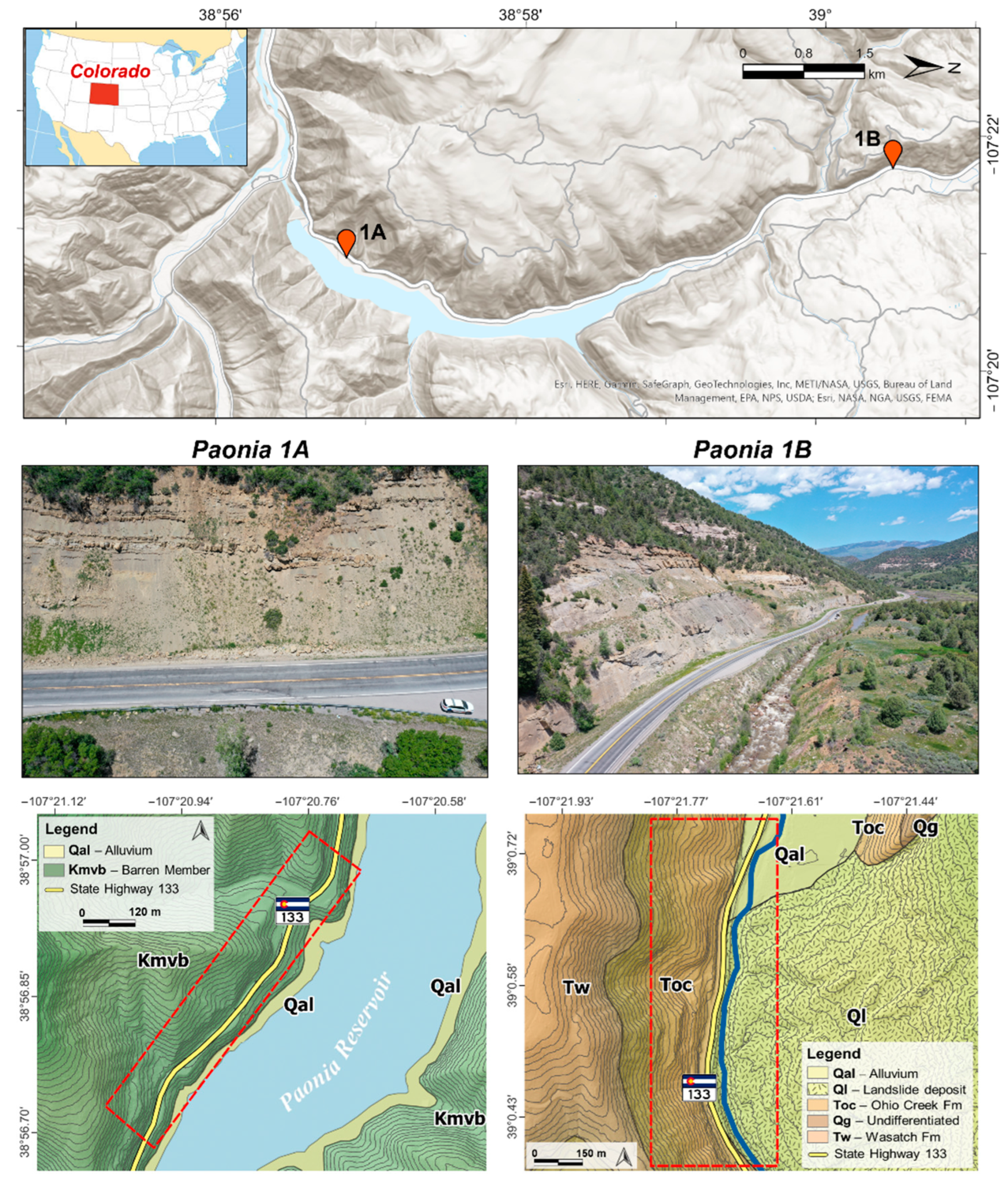
2. Geographical and Geological Settings
3. Materials and Methods
3.1. Satellite-Based (InSAR) Analysis
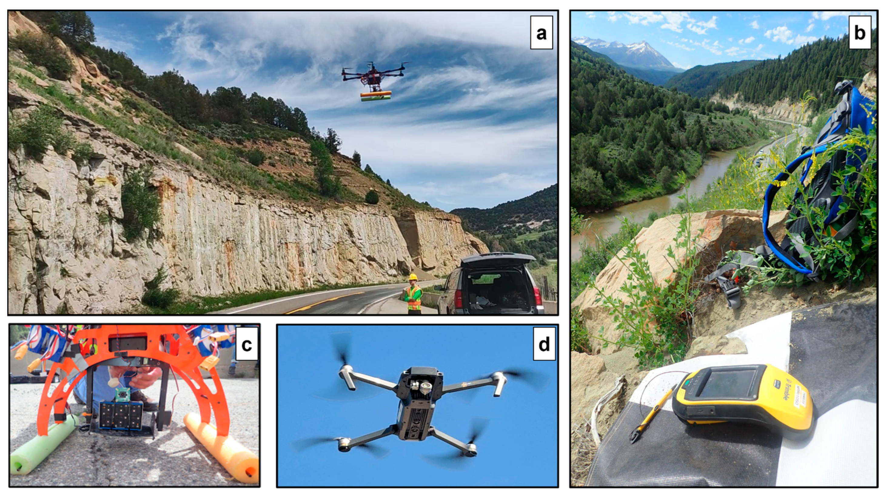
3.2. UAS-Based Acquisition and Processing
3.2.1. Pre-Processing
3.2.2. Processing: Classification Analysis
3.2.3. Processing: Change Detection Analysis
4. Results
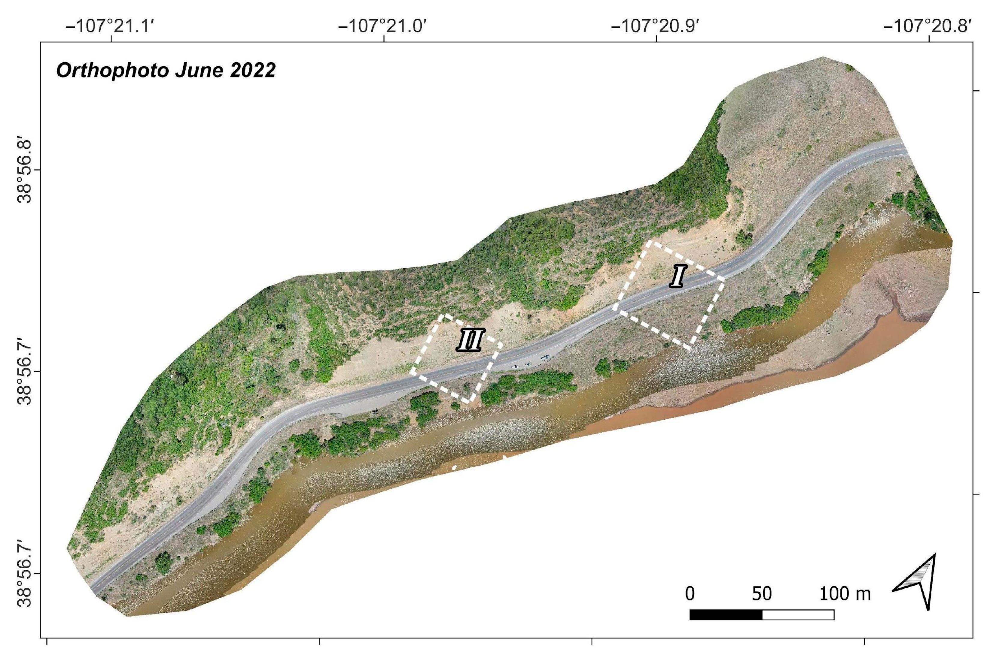
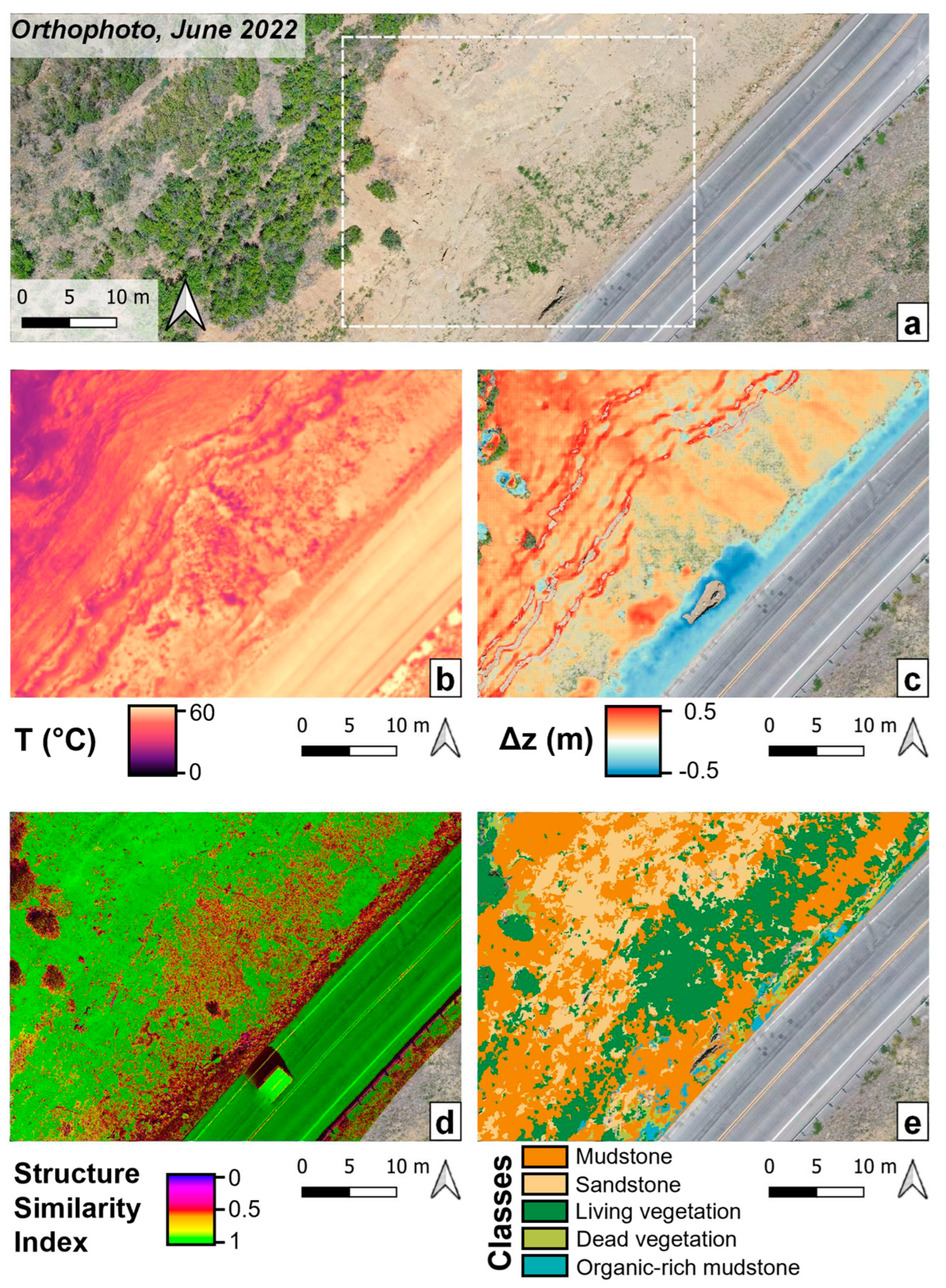
4.1. Paonia 1A
4.2. Paonia 1B
5. Discussion
6. Conclusions
- The combination of different platforms (satellite or UAS) and sensors, along with their respective products at varying spatial resolutions, was essential to identify several superimposed processes. Each informative level (i.e., multispectral and SAR analysis, thermal and optical products, terrain models), enabled distinguishing the specific geomorphic expression of the different degradation processes. In doing so, we shed light on the landform’s multi-scale characteristics, thus interpreting their potential to differentially disrupt the slope stability. Moreover, the examples of retrogressive erosion and rill initiation retrieved in both study areas represent early predictorsof future rock failures or road collapses.
- The fourth dimension (i.e., time), explored through the use of multi-temporal data collections, provides a significant amplification of the potential of a single remote sensing survey. Change detection and interferometric analyses allowed the quantitative assessment of the dynamics of morphological features (e.g., road crack propagation, areas more susceptible to depletion or sediment accumulation) and a preliminary forecast of their morphoevolution.
- Unusual processing solutions, such as optical-based change detection, can lead to new opportunities for micro-morphotype detection and characterization. This technique could serve as a primary step for a more quantitative assessment of the slope erosion rates and geostructural stability.
- Remote sensing data can provide a detailed model of the slope’s mechanics and conditions at a specific time. This information is particularly beneficial for monitoring highway networks and transportation corridors, supporting asset management practices from a predictive maintenance perspective.
Author Contributions
Funding
Data Availability Statement
Acknowledgments
Conflicts of Interest
References
- Agliardi, F.; Crosta, G.B. High resolution three-dimensional numerical modelling of rockfalls. Int. J. Rock Mech. Min. Sci. 2003, 40, 455–471. [Google Scholar] [CrossRef]
- Martino, S.; Bozzano, F.; Caporossi, P.; D’angiò, D.; Della Seta, M.; Esposito, C.; Fantini, A.; Fiorucci, M.; Giannini, L.M.; Iannucci, R.; et al. Impact of landslides on transportation routes during the 2016–2017 Central Italy seismic sequence. Landslides 2019, 16, 1221–1241. [Google Scholar] [CrossRef]
- Landslides 101|U.S. Geological Survey. Available online: https://www.usgs.gov/programs/landslide-hazards/landslides-101 (accessed on 20 March 2023).
- Lato, M.J.; Gauthier, D.; Hutchinson, D.J. Rock Slopes Asset Management: Selecting the Optimal Three-Dimensional Remote Sensing Technology. Transp. Res. Rec. 2015, 2510, 7–14. [Google Scholar] [CrossRef]
- Arpin, B.; Arndt, B. Comparison of 2D and 3D rockfall modeling for rockfall mitigation design. In Proceedings of the 67th Highway Geology Symposium, Highway Geology Symposium, Colorado Springs, CO, USA, 11–14 July 2016. [Google Scholar]
- Guzzetti, F. Landslide fatalities and the evaluation of landslide risk in Italy. Eng. Geol. 2000, 58, 89–107. [Google Scholar] [CrossRef]
- Crosta, G.B.; Agliardi, F. A methodology for physically based rockfall hazard assessment. Nat. Hazards Earth Syst. Sci. 2003, 3, 407–422. [Google Scholar] [CrossRef]
- Piacentini, D.; Ercolessi, G.; Pizziolo, M.; Troiani, F. Rockfall runout, Mount Cimone area, Emilia-Romagna Region, Italy. J. Maps 2015, 11, 598–605. [Google Scholar] [CrossRef]
- Moore, J.R.; Sanders, J.W.; Dietrich, W.E.; Glaser, S.D. Influence of rock mass strength on the erosion rate of alpine cliffs. Earth Surf. Process. Landf. 2009, 34, 1339–1352. [Google Scholar] [CrossRef]
- Karir, D.; Ray, A.; Bharati, A.K.; Chaturvedi, U.; Rai, R.; Khandelwal, M. Stability prediction of a natural and man-made slope using various machine learning algorithms. Transp. Geotech. 2022, 34, 100745. [Google Scholar] [CrossRef]
- Khorram, S.; Nelson, S.A.; Koch, F.H.; van der Wiele, C.F. Remote Sensing; Springer Science & Business Media: Berlin/Heidelberg, Germany, 2012. [Google Scholar] [CrossRef]
- Rosi, A.; Tofani, V.; Tanteri, L.; Tacconi Stefanelli, C.; Agostini, A.; Catani, F.; Casagli, N. The new landslide inventory of Tuscany (Italy) updated with PS-InSAR: Geomorphological features and landslide distribution. Landslides 2018, 15, 5–19. [Google Scholar] [CrossRef]
- Dini, B.; Manconi, A.; Loew, S. Investigation of slope instabilities in NW Bhutan as derived from systematic DInSAR analyses. Eng. Geol. 2019, 259, 105111. [Google Scholar] [CrossRef]
- Hussain, M.A.; Chen, Z.; Wang, R.; Shoaib, M. PS-InSAR-Based Validated Landslide Susceptibility Mapping along Karakoram Highway, Pakistan. Remote Sens. 2021, 13, 4129. [Google Scholar] [CrossRef]
- Yuan, R.; Chen, J. A hybrid deep learning method for landslide susceptibility analysis with the application of InSAR data. Nat. Hazards 2022, 114, 1393–1426. [Google Scholar] [CrossRef]
- Lucieer, A.; Jong, S.M.D.; Turner, D. Mapping landslide displacements using Structure from Motion (SfM) and image correlation of multi-temporal UAV photography. Prog. Phys. Geogr. 2013, 38, 97–116. [Google Scholar] [CrossRef]
- Wang, W.; Zhao, W.; Chai, B.; Du, J.; Tang, L.; Yi, X. Discontinuity interpretation and identification of potential rockfalls for high-steep slopes based on UAV nap-of-the-object photogrammetry. Comput. Geosci. 2022, 166, 105191. [Google Scholar] [CrossRef]
- Ismail, A.; Rashid, A.A.S.; Sa’ari, R.; Rasib, A.W.; Mustaffar, M.; Abdullah, R.A.; Kassim, A.; Mohd Yusof, N.; Abd Rahaman, N.; Mohd Apandi, N.; et al. Application of UAV-based photogrammetry and normalised water index (NDWI) to estimate the rock mass rating (RMR): A case study. Phys. Chem. Earth Parts A/B/C 2022, 127, 103161. [Google Scholar] [CrossRef]
- Filice, F.; Pezzo, A.; Lollino, P.; Perrotti, M.; Ietto, F. Multi-approach for the assessment of rock slope stability using in-field and UAV investigations. Bull. Eng. Geol. Environ. 2022, 81, 502. [Google Scholar] [CrossRef]
- Robiati, C.; Eyre, M.; Vanneschi, C.; Francioni, M.; Venn, A.; Coggan, J. Application of Remote Sensing Data for Evaluation of Rockfall Potential within a Quarry Slope. ISPRS Int. J. Geo-Inf. 2019, 8, 367. [Google Scholar] [CrossRef]
- Stead, D.; Donati, D.; Wolter, A.; Sturzenegger, M. Application of Remote Sensing to the Investigation of Rock Slopes: Experience Gained and Lessons Learned. ISPRS Int. J. Geo-Inf. 2019, 8, 296. [Google Scholar] [CrossRef]
- Devoto, S.; Macovaz, V.; Mantovani, M.; Soldati, M.; Furlani, S. Advantages of Using UAV Digital Photogrammetry in the Study of Slow-Moving Coastal Landslides. Remote Sens. 2020, 12, 3566. [Google Scholar] [CrossRef]
- Ismail, A.; Ahmad Safuan, A.R.; Sa’ari, R.; Wahid Rasib, A.; Mustaffar, M.; Asnida Abdullah, R.; Kassim, A.; Mohd Yusof, N.; Abd Rahaman, N.; Kalatehjari, R. Application of combined terrestrial laser scanning and unmanned aerial vehicle digital photogrammetry method in high rock slope stability analysis: A case study. Meas. J. Int. Meas. Confed. 2022, 195, 111161. [Google Scholar] [CrossRef]
- Gantimurova, S.; Parshin, A.; Erofeev, V. GIS-Based Landslide Susceptibility Mapping of the Circum-Baikal Railway in Russia Using UAV Data. Remote Sens. 2021, 13, 3629. [Google Scholar] [CrossRef]
- Konstantinidis, I.; Marinos, V.; Papathanassiou, G. UAV-Based Evaluation of Rockfall Hazard in the Cultural Heritage Area of Kipinas Monastery, Greece. Appl. Sci. 2021, 11, 8946. [Google Scholar] [CrossRef]
- Udin, W.S.; Norazami, N.A.S.; Sulaiman, N.; Zaudin, N.C.; Ma’ail, S.; Nor, A.M. UAV based multi-spectral imaging system for mapping landslide risk area along Jeli-Gerik highway, Jeli, Kelantan. In Proceedings of the 2019 IEEE 15th International Colloquium on Signal Processing & Its Applications (CSPA), Pulau Pinang, Malaysia, 8–9 March 2019; pp. 162–167. [Google Scholar] [CrossRef]
- Wang, S.; Zhang, Z.; Wang, C.; Zhu, C.; Ren, Y. Multistep rocky slope stability analysis based on unmanned aerial vehicle photogrammetry. Environ. Earth Sci. 2019, 78, 260. [Google Scholar] [CrossRef]
- Robiati, C.; Mastrantoni, G.; Francioni, M.; Eyre, M.; Coggan, J.; Mazzanti, P. Contribution of High-Resolution Virtual Outcrop Models for the Definition of Rockfall Activity and Associated Hazard Modelling. Land 2023, 12, 191. [Google Scholar] [CrossRef]
- Lin, J.; Wang, M.; Yang, J.; Yang, Q. Landslide identification and information extraction based on optical and multispectral UAV remote sensing imagery. In IOP Conference Series: Earth and Environmental Science; IOP Publishing: Beijing, China, 2016; Volume 57, p. 012017. [Google Scholar]
- He, J.; Barton, I. Hyperspectral remote sensing for detecting geotechnical problems at Ray mine. Eng. Geol. 2019, 292, 106261. [Google Scholar] [CrossRef]
- Frodella, W.; Gigli, G.; Morelli, S.; Lombardi, L.; Casagli, N. Landslide Mapping and Characterization through Infrared Thermography (IRT): Suggestions for a Methodological Approach from Some Case Studies. Remote Sens. 2017, 9, 1281. [Google Scholar] [CrossRef]
- Abellán, A.; Calvet, J.; Vilaplana, J.M.; Blanchard, J. Detection and spatial prediction of rockfalls by means of terrestrial laser scanner monitoring. Geomorphology 2010, 119, 162–171. [Google Scholar] [CrossRef]
- Royán, M.J.; Abellán, A.; Jaboyedoff, M.; Vilaplana, J.M.; Calvet, J. Spatio-temporal analysis of rockfall pre-failure deformation using Terrestrial LiDAR. Landslides 2014, 11, 697–709. [Google Scholar] [CrossRef]
- Kromer, R.A.; Hutchinson, D.J.; Lato, M.J.; Gauthier, D.; Edwards, T. Identifying rock slope failure precursors using LiDAR for transportation corridor hazard management. Eng. Geol. 2015, 195, 93–103. [Google Scholar] [CrossRef]
- Farmakis, I.; Marinos, V.; Papathanassiou, G.; Karantanellis, E. Automated 3D Jointed Rock Mass Structural Analysis and Characterization Using LiDAR Terrestrial Laser Scanner for Rockfall Susceptibility Assessment: Perissa Area Case (Santorini). Geotech. Geol. Eng. 2020, 38, 3007–3024. [Google Scholar] [CrossRef]
- Núñez-Andrés, M.A.; Prades-Valls, A.; Matas, G.; Buill, F.; Lantada, N. New Approach for Photogrammetric Rock Slope Premonitory Movements Monitoring. Remote Sens. 2023, 15, 293. [Google Scholar] [CrossRef]
- Carlà, T.; Nolesini, T.; Solari, L.; Rivolta, C.; Dei Cas, L.; Casagli, N. Rockfall forecasting and risk management along a major transportation corridor in the Alps through ground-based radar interferometry. Landslides 2019, 16, 1425–1435. [Google Scholar] [CrossRef]
- Romeo, S.; Cosentino, A.; Giani, F.; Mastrantoni, G.; Mazzanti, P. Combining Ground Based Remote Sensing Tools for Rockfalls Assessment and Monitoring: The Poggio Baldi Landslide Natural Laboratory. Sensors 2021, 21, 2632. [Google Scholar] [CrossRef]
- Graber, A.; Santi, P. UAV-photogrammetry rockfall monitoring of natural slopes in Glenwood Canyon, CO, USA: Background activity and post-wildfire impacts. Landslides 2023, 20, 229–248. [Google Scholar] [CrossRef]
- Sarro, R.; Riquelme, A.; García-Davalillo, J.C.; Mateos, R.M.; Tomás, R.; Pastor, J.L.; Herrera, G. Rockfall Simulation Based on UAV Photogrammetry Data Obtained during an Emergency Declaration: Application at a Cultural Heritage Site. Remote Sens. 2018, 10, 1923. [Google Scholar] [CrossRef]
- Francioni, M.; Antonaci, F.; Sciarra, N.; Robiati, C.; Coggan, J.; Stead, D.; Calamita, F. Application of Unmanned Aerial Vehicle Data and Discrete Fracture Network Models for Improved Rockfall Simulations. Remote Sens. 2020, 12, 2053. [Google Scholar] [CrossRef]
- Gallo, I.G.; Martínez-Corbella, M.; Sarro, R.; Iovine, G.; López-Vinielles, J.; Hérnandez, M.; Robustelli, G.; Mateos, R.M.; García-Davalillo, J.C. An Integration of UAV-Based Photogrammetry and 3D Modelling for Rockfall Hazard Assessment: The Cárcavos Case in 2018 (Spain). Remote Sens. 2021, 13, 3450. [Google Scholar] [CrossRef]
- Žabota, B.; Berger, F.; Kobal, M. The Potential of UAV-Acquired Photogrammetric and LiDAR-Point Clouds for Obtaining Rock Dimensions as Input Parameters for Modeling Rockfall Runout Zones. Drones 2023, 7, 104. [Google Scholar] [CrossRef]
- Migliazza, M.; Carriero, M.T.; Lingua, A.; Pontoglio, E.; Scavia, C. Rock Mass Characterization by UAV and Close-Range Photogrammetry: A Multiscale Approach Applied along the Vallone dell’Elva Road (Italy). Geosciences 2021, 11, 436. [Google Scholar] [CrossRef]
- Rodriguez, J.; Macciotta, R.; Hendry, M.T.; Roustaei, M.; Gräpel, C.; Skirrow, R. UAVs for monitoring, investigation, and mitigation design of a rock slope with multiple failure mechanisms—A case study. Landslides 2020, 17, 2027–2040. [Google Scholar] [CrossRef]
- Caliò, D.; Mineo, S.; Pappalardo, G. Digital Rock Mass Analysis for the Evaluation of Rockfall Magnitude at Poorly Accessible Cliffs. Remote Sens. 2023, 15, 1515. [Google Scholar] [CrossRef]
- Liu, Z.; Qiu, H.; Ma, S.; Yang, D.; Pei, Y.; Du, C.; Sun, H.; Hu, S.; Zhu, Y. Surface displacement and topographic change analysis of the Changhe landslide on September 14, 2019, China. Landslides 2021, 18, 1471–1483. [Google Scholar] [CrossRef]
- Ma, S.; Qiu, H.; Hu, S.; Yang, D.; Liu, Z. Characteristics and geomorphology change detection analysis of the Jiangdingya landslide on July 12, 2018, China. Landslides 2021, 18, 383–396. [Google Scholar] [CrossRef]
- Hu, S.; Qiu, H.; Wang, N.; Wang, X.; Ma, S.; Yang, D.; Wei, N.; Liu, Z.; Shen, Y.; Cao, M.; et al. Movement process, geomorphological changes, and influencing factors of a reactivated loess landslide on the right bank of the middle of the Yellow River, China. Landslides 2022, 19, 1265–1295. [Google Scholar] [CrossRef]
- Liu, Z.; Qiu, H.; Zhu, Y.; Liu, Y.; Yang, D.; Ma, S.; Zhang, J.; Wang, Y.; Wang, L.; Tang, B. Efficient Identification and Monitoring of Landslides by Time-Series InSAR Combining Single- and Multi-Look Phases. Remote Sens. 2022, 14, 1026. [Google Scholar] [CrossRef]
- Johnson, R.C.; May, F. A study of the Cretaceous-Tertiary unconformity in the Piceance Creek Basin, Colorado: The underlying Ohio Creek Formation (Upper Cretaceous) redefined as a member of the Hunter Canyon or Mesaverde Formation. Geol. Surv. Bull. 1980, 1482-B. [Google Scholar]
- Godwin, L.H. Geologic Map of the Chair Mountain Quadrangle, Gunnison and Pitkin Counties, Colorado; (No. 704); USGA: Reston, VA, USA, 1968. [Google Scholar] [CrossRef]
- Johnson, R.C. Geologic History and Hydrocarbon Potential of Late Cretaceous-Age, Low-Permeability Reservoirs, Piceance Basin, Western Colorado; (No. 1787-E); USGA: Reston, VA, USA, 1989. [Google Scholar] [CrossRef]
- Dunrud, C.R. Geologic Map and Coal Stratigraphic Framework of the Paonia Area, Delta and Gunnison Counties, Colorado; (No. 115); USGA: Reston, VA, USA, 1989. [Google Scholar] [CrossRef]
- Aswathi, J.; Binoj Kumar, R.B.; Oommen, T.; Bouali, E.H.; Sajinkumar, K.S. InSAR as a tool for monitoring hydropower projects: A review. Energy Geosci. 2022, 3, 160–171. [Google Scholar] [CrossRef]
- Ferretti, A.; Prati, C.; Rocca, F. Permanent scatterers in SAR interferometry. IEEE Trans. Geosci. Remote Sens. 2001, 39, 8–20. [Google Scholar] [CrossRef]
- Funning, G.J.; Bürgmann, R.; Ferretti, A.; Novali, F.; Fumagalli, A. Creep on the Rodgers Creek fault, northern San Francisco Bay area from a 10 year PS-InSAR dataset. Geophys. Res. Lett. 2007, 34. [Google Scholar] [CrossRef]
- Perissin, D.; Wang, Z.; Wang, T. The SARPROZ InSAR tool for urban subsidence/manmade structure stability monitoring in China. In Proceedings of the 34th International Symposium of Remote Sensing of Environment, Sidney, Australia, 10–15 April 2011. [Google Scholar]
- Antonielli, B.; Sciortino, A.; Scancella, S.; Bozzano, F.; Mazzanti, P. Tracking Deformation Processes at the Legnica Glogow Copper District (Poland) by Satellite InSAR—I: Room and Pillar Mine District. Land 2021, 10, 653. [Google Scholar] [CrossRef]
- Moretto, S.; Bozzano, F.; Mazzanti, P. The Role of Satellite InSAR for Landslide Forecasting: Limitations and Openings. Remote Sens. 2021, 13, 3735. [Google Scholar] [CrossRef]
- Trimble Germany GmbH. Trimble Documentation eCognition Developer 10.1 User Guide; Trimble Germany GmbH: Munich, Germany, 2022. [Google Scholar]
- Blaschke, T. Object based image analysis for remote sensing. ISPRS J. Photogramm. Remote Sens. 2010, 65, 2–16. [Google Scholar] [CrossRef]
- Hussain, M.; Chen, D.; Cheng, A.; Wei, H.; Stanley, D. Change detection from remotely sensed images: From pixel-based to object-based approaches. ISPRS J. Photogramm. Remote Sens. 2013, 80, 91–106. [Google Scholar] [CrossRef]
- Asokan, A.; Anitha, J.J.E.S.I. Change detection techniques for remote sensing applications: A survey. Earth Sci. Inform. 2019, 12, 143–160. [Google Scholar] [CrossRef]
- Photomonitoring.com. Available online: https://www.photomonitoring.com/iris/ (accessed on 25 April 2023).
- Wang, Z.; Bovik, A.C.; Sheikh, H.R.; Simoncelli, E.P. Image Quality Assessment: From Error Visibility to Structural Similarity. IEEE Trans. Image Process. 2004, 13, 600–612. [Google Scholar] [CrossRef]
- Cosentino, A.; Brunetti, A.; Fiorio, M.; Gaeta, M.; Mazzanti, P. IRIS a new powerful tool for Geohazards Assessment by PhotoMonitoring. In Proceedings of the Asita Conference, Genova, Italy, 20–24 June 2022. [Google Scholar]
- Mazzanti, P.; Scancella, S.; Virelli, M.; Frittelli, S.; Nocente, V.; Lombardo, F. Assessing the Performance of Multi-Resolution Satellite SAR Images for Post-Earthquake Damage Detection and Mapping Aimed at Emergency Response Management. Remote Sens. 2022, 14, 2210. [Google Scholar] [CrossRef]
- Stover, B.K. Surficial-Geologic Map of the Muddy Creek Landslide Complex, Gunnison County, Colorado, April 15, 1986; Surface Geologic, Open File Report; Colorado Geological Survey, Department of Natural Resources: Denver, CO, USA, 1986. Available online: https://coloradogeologicalsurvey.org/publications/surficial-geologic-map-muddy-creek-landslide-complex-gunnison-colorado-1986/ (accessed on 6 June 2023).
- Lowry, B.W.; Baker, S.; Zhou, W. A Case Study of Novel Landslide Activity Recognition Using ALOS-1 InSAR within the Ragged Mountain Western Hillslope in Gunnison County, Colorado, USA. Remote Sens. 2020, 12, 1969. [Google Scholar] [CrossRef]
- U.S. Geological Survey. 3D Elevation Program 1-Meter Resolution Digital Elevation Model (Published 20200606). 2019. Available online: https://www.usgs.gov/the-national-map-data-delivery (accessed on 24 April 2023).
- Weatherwx.com. Available online: https://www.weatherwx.com/climate-averages/co/paonia+reservoir.html (accessed on 24 April 2023).
- Schmidt, J.; Andrew, R. Multi-scale landform characterization. Area 2005, 37, 341–350. [Google Scholar] [CrossRef]
- El Hajj, M.; Baghdadi, N.; Zribi, M. Comparative analysis of the accuracy of surface soil moisture estimation from the C- and L-bands. Int. J. Appl. Earth Obs. Geoinf. 2019, 82, 101888. [Google Scholar] [CrossRef]
- Draebing, D. Identification of rock and fracture kinematics in high alpine rockwalls under the influence of elevation. Earth Surf. Dyn. 2021, 9, 977–994. [Google Scholar] [CrossRef]
- Birien, T.; Gauthier, F. Influence of climate-dependent variables on deformation and differential erosion of stratified sedimentary rocks. Geomorphology 2023, 421, 108518. [Google Scholar] [CrossRef]
- Santi, P.M.; Russell, C.P.; Higgins, J.D.; Spriet, J.I. Modification and statistical analysis of the Colorado Rockfall Hazard Rating System. Eng. Geol. 2009, 104, 55–65. [Google Scholar] [CrossRef]
- Oommen, T.; Vitton, S.; Escobar-Wolf, R.; Brooks, C. Rockfall Hazard Rating System: Benefits of Utilizing Remote Sensing. Environ. Eng. Geosci. 2017, 23, 165–177. [Google Scholar] [CrossRef]


| Characteristics | DJI Mavic 2 Pro | DJI M2EA | Bergen Hexacopter |
|---|---|---|---|
| Camera | Integrated 20 MP | Integrated dual optical (12/48 MP) thermal (640 × 480 radiometric 30 Hz) | Tetracam Micro-MCA6 |
| Maximum take-off weight (kg) | 0.907 | 0.11 | 4.5 |
| Flight range (min) | 25 | 25 | 15 |
| Flight altitude (m) | 45–60 | 30–60 | 30–70 |
| Maximum horizontal speed (km/h) | 72 | 72 | 30 |
| N° of images (nadir) | 2000 | 3500 thermal | Tetracam: 700 (6 bands) |
| N° of images (oblique) | 800 | 900 thermal | Tetracam: 500 (6 bands) |
| Sensor | Type of Product | Scale | Type of Process or Landform |
|---|---|---|---|
| Satellite Radar (C band) | PS-InSAR analysis | Catchment or sub-catchment scale | Large landslides and deformations |
| Mavic 2 Pro integrated 20 mp | DEM-based change detection | Hillslope scale | Sediment accumulation and erosional processes |
| M2EA thermal | Thermal imagery | Hillslope scale | Humid zone and rock differentiation |
| Mavic 2 Pro integrated 20 mp | Optical imagery | Sub-hillslope scale | Small-scale topographic features |
| Mavic 2 Pro integrated 20 mp | Optical imagery-based change detection | Micro-topography scale | Rills and road crack formation or opening |
| Tetracam Micro-MCA6 | Multispectral analysis | Sub-hillslope scale | Small-scale rock and soil differentiation |
| Micro-topography scale | Seep area identification |
Disclaimer/Publisher’s Note: The statements, opinions and data contained in all publications are solely those of the individual author(s) and contributor(s) and not of MDPI and/or the editor(s). MDPI and/or the editor(s) disclaim responsibility for any injury to people or property resulting from any ideas, methods, instructions or products referred to in the content. |
© 2023 by the authors. Licensee MDPI, Basel, Switzerland. This article is an open access article distributed under the terms and conditions of the Creative Commons Attribution (CC BY) license (https://creativecommons.org/licenses/by/4.0/).
Share and Cite
Zocchi, M.; Kasaragod, A.K.; Jenkins, A.; Cook, C.; Dobson, R.; Oommen, T.; Van Huis, D.; Taylor, B.; Brooks, C.; Marini, R.; et al. Multi-Sensor and Multi-Scale Remote Sensing Approach for Assessing Slope Instability along Transportation Corridors Using Satellites and Uncrewed Aircraft Systems. Remote Sens. 2023, 15, 3016. https://doi.org/10.3390/rs15123016
Zocchi M, Kasaragod AK, Jenkins A, Cook C, Dobson R, Oommen T, Van Huis D, Taylor B, Brooks C, Marini R, et al. Multi-Sensor and Multi-Scale Remote Sensing Approach for Assessing Slope Instability along Transportation Corridors Using Satellites and Uncrewed Aircraft Systems. Remote Sensing. 2023; 15(12):3016. https://doi.org/10.3390/rs15123016
Chicago/Turabian StyleZocchi, Marta, Anush Kumar Kasaragod, Abby Jenkins, Chris Cook, Richard Dobson, Thomas Oommen, Dana Van Huis, Beau Taylor, Colin Brooks, Roberta Marini, and et al. 2023. "Multi-Sensor and Multi-Scale Remote Sensing Approach for Assessing Slope Instability along Transportation Corridors Using Satellites and Uncrewed Aircraft Systems" Remote Sensing 15, no. 12: 3016. https://doi.org/10.3390/rs15123016
APA StyleZocchi, M., Kasaragod, A. K., Jenkins, A., Cook, C., Dobson, R., Oommen, T., Van Huis, D., Taylor, B., Brooks, C., Marini, R., Troiani, F., & Mazzanti, P. (2023). Multi-Sensor and Multi-Scale Remote Sensing Approach for Assessing Slope Instability along Transportation Corridors Using Satellites and Uncrewed Aircraft Systems. Remote Sensing, 15(12), 3016. https://doi.org/10.3390/rs15123016