Article

Supervised Classification of Tree Cover Classes in the Complex Mosaic Landscape of Eastern Rwanda

1
Division of Forest, Nature and Landscape, KU Leuven, 3000 Leuven, Belgium
2
Flemish Institute for Technological Research (VITO), 2400 Mol, Belgium
*
Author to whom correspondence should be addressed.
Remote Sens. 2023, 15(10), 2606; https://doi.org/10.3390/rs15102606
Submission received: 20 March 2023 / Revised: 12 May 2023 / Accepted: 15 May 2023 / Published: 17 May 2023
(This article belongs to the Section Forest Remote Sensing)

Abstract

:
Eastern Rwanda consists of a mosaic of different land cover types, with agroforestry, forest patches, and shrubland all containing tree cover. Mapping and monitoring the landscape is costly and time-intensive, creating a need for automated methods using openly available satellite imagery. Google Earth Engine and the random forests algorithm offer the potential to use such imagery to map tree cover types in the study area. Sentinel-2 satellite imagery, along with vegetation indices, texture metrics, principal components, and non-spectral layers were combined over the dry and rainy seasons. Different combinations of input bands were used to classify land cover types in the study area. Recursive feature elimination was used to select the most important input features for accurate classification, with three final models selected for classification. The highest classification accuracies were obtained for the forest class (85–92%) followed by shrubland (77–81%) and agroforestry (68–77%). Agroforestry cover was predicted for 36% of the study area, forest cover was predicted for 14% of the study area, and shrubland cover was predicted for 18% of the study area. Non-spectral layers and texture metrics were among the most important features for accurate classification. Mixed pixels and fragmented tree patches presented challenges for the accurate delineation of some tree cover types, resulting in some discrepancies with other studies. Nonetheless, the methods used in this study were capable of delivering accurate results across the study area using freely available satellite imagery and methods that are not costly and are easy to apply in future studies.

Graphical Abstract

1. Introduction

Population pressure and shifting agriculture have been key drivers of tree cover loss in sub-Saharan Africa, where there has been a decline in forest cover from approximately 6.7 million km2 in 1990 to 5.9 million km2 in 2015, a decrease of about 12% [1,2,3]. The complex interaction between forest ecosystems and human agricultural and urban systems is particularly important in Africa, where human pressure drives deforestation through the gathering of firewood, charcoal production, mining, and shifting agriculture [4]. As a small, landlocked country with the highest population density in Africa (over 500 people/km2), Rwanda faces many challenges with regard to the balance between natural ecosystems and human land use. A rapidly growing population, as well as traditional inheritance practices, have created a complex mosaic landscape of different land uses, mainly blending forms of agriculture and forestry [5].
The semi-arid eastern region of Rwanda is characterized by relatively low annual rainfall with both mixed agriculture and agropastoralism playing key roles in the livelihoods of rural residents [6]. In this region, tree cover at landscape level is present in three land cover classes, namely forests, agroforestry, and shrublands. Forests consist largely of managed plantations with large variations in productivity. Poorly managed private forests often face degradation due to overharvesting of wood resources by rural populations [7]. Forests, as well as isolated trees, are vital for the sustenance of local economies through the provision of non-timber forest products and firewood for energy, cooking, and charcoal for both rural and urban populations. Such practices are important for many rural inhabitants, contributing directly to household incomes. However, very few households can rely on this income due to the fragmentation of forests within the larger landscape dominated by agriculture [8,9,10]. The combination of high population densities and widespread smallholder agriculture has ensured that forests remain fragmented and are thus not a significant source of firewood resources to much of the rural population [11]. Thus, much of the firewood is obtained through agroforestry, a common practice with rural populations in the country.
Agroforestry is a land cover type with a mixture of agriculture and trees, including scattered trees on farms. In Rwanda, the application of agroforestry methods has led to the restoration of degraded lands, improvement in soil quality, and higher living standards for farmers [12]. Furthermore, such systems have been a part of agricultural practices in Rwanda for centuries [13]. Shrubs, or smaller, woody perennials, are a key source of fuel for cooking and energy purposes, and are especially prevalent in the northeastern savannah agroecological zone [6,11,14]. Shrublands, a semi-arid land cover type featuring natural trees and smaller shrubs in a savannah-like environment, are severely degraded in Rwanda, despite their importance as a source of woody biomass for rural populations [15]. This degradation comes as a result of the conversion of shrubland to agricultural land, which can lead to a decrease in woody biomass provision, as well as negative impacts on carbon storage and water yield [16]. Shrubs are also used extensively in agroforestry systems, as their smaller size ensures they can be incorporated more easily with existing cropland [17]. Ongoing government initiatives aim to integrate agroforestry techniques and practices in the farming system to increase the availability of tree resources for rural populations and diversify farmer incomes [7]. Unsustainable harvesting practices threaten the long-term supply of woody biomass for rural populations in Rwanda, a trend that is aggravated by the lack of consistent monitoring methods to prevent the overexploitation of tree resources [18].
The lack of accurate and continuous monitoring methods is a key hindrance for evaluating the effectiveness of efforts to increase woody biomass through the planting of trees in forests and agroforestry plots. In this challenge, state-of-the art satellite imagery and automated machine learning algorithms may provide a potential solution that is both accurate and low-cost. Previous research to model the vegetation dynamics in Rwanda has mostly used Landsat satellite imagery with a 30 m resolution, which is often too coarse to accurately map the very small parcel sizes of smallholder farms and the fragmented patches of forest [19,20,21,22,23]. A more recent study used very high-resolution (0.25 m) aerial imagery together with deep learning methods to map individual tree crowns in Rwanda, attaining high pixel accuracy rates of up to 96% [24]. However, the imagery acquired for the previous study is rare and expensive to acquire, limiting the repeatability of such research. There have not been any previous studies delineating or classifying tree cover in Rwanda using Sentinel-2 (S2) imagery, which is more cost-effective and has a higher resolution than Landsat imagery.
S2 imagery has been used extensively for mapping forest cover and classifying land cover type in different regions across the world [25]. Due to the medium resolution (10 m) of this imagery, past studies have used satellite imagery with a higher resolution to identify locations for training data for the classification of small tree plantations and shrubland vegetation cover [26,27]. Previous research in mosaic landscapes with small farm plots suggests that medium-resolution data, such as that provided by S2, can deliver accurate tree cover results for the benefit of both researchers and local stakeholders [28]. The use of vegetation indices has also been shown to improve the accuracy of classification studies at differentiating land cover types in arid regions [26,29]. For example, the normalized difference vegetation index (NDVI) has been shown to increase the differentiation of vegetation from other land covers such as soil [30], while other indices are also effective [31]. Furthermore, additional input layers such as texture metrics have also been successfully used to improve classification results in complex landscapes [32]. In a mosaic landscape, additional layers can provide a contrast between different land cover types and improve the classification accuracy for mixed land cover pixels. However, very large input datasets can limit RF model performance, so feature selection methods are necessary to reduce to size of an input dataset and reduce input layer redundancy [33,34].
The combination of both multispectral datasets along with vegetation indices, texture metrics, and non-spectral layers, an approach now common in land cover studies, requires robust and accurate classification algorithms. Machine learning methods improve results compared to traditional regression and parametric methods. Commonly used machine learning classification algorithms include decision trees, support vector machines, artificial neural networks, and random forests (RF) [27]. Random forests uses a set of decision-making ‘trees’ to perform classification and generate accurate results with less noise than single tree classifiers, resulting in their extensive application in classification studies [25]. This model is commonly used in remote sensing studies because it can handle large amounts of data with a small computational load while reducing biases and noise [35]. However, studies have shown that RF requires sizeable training datasets, reaching higher accuracies at a minimum of 500–1000 training pixels per class [36,37].
The complexity and computational requirements for processing large multispectral datasets necessitate methods that allow the user to perform calculations in an efficient and accessible manner. Google Earth Engine (GEE) is a cloud-based platform that allows the user to perform complex calculations using massive amounts of data on a network of machines managed by Google [38]. GEE’s lazy evaluation methods, which delay processing until a result is requested, combined with cloud computation, allow for the testing and development of algorithms for land cover classification without the time and computational power required by traditional machines [39]. The processing power, together with the ease of access to myriad high-quality, multitemporal spatial datasets have played key roles in the growing popularity of GEE in recent years [40].
This study aims to use machine learning methods to classify publicly available S2 imagery in eastern Rwanda. We will use GEE to apply supervised pixel-based classification algorithms to large, multispectral datasets in order to identify tree cover in a complex, mosaic landscape. We aim to improve on past studies in this region by developing a higher-resolution final product, with express focus on the specific land cover types which feature trees in eastern Rwanda. This study aims to answer the following questions:
  • Which methods and input layers lead to the most accurate land cover classification model for eastern Rwanda?
  • What is the spatial extent and distribution of the main land cover types that feature trees in the study area?
  • How does the distribution of these land cover types relate to rural populations, and what implications does this have for sustainable wood harvests in the study area?
This study will use publicly available imagery and pixel-based classification methods to answer the above questions.

2. Materials and Methods

2.1. Study Area

The study area comprises the Eastern Province of Rwanda as well as the peri-urban areas surrounding the capital city of Kigali (Figure 1). The Eastern Province is divided into seven districts, and the capital city region into three districts. The total study area is 10,194 km2, which is approximately 39% of the entire country area and lies between 29°57′E and 30°55′E latitude and 1°1′S and 2°26′S longitude. Rwanda is a landlocked country in Central/East Africa, sharing borders with the Democratic Republic of the Congo, Uganda, Tanzania, and Burundi. The country has a population of over 13.2 million people, of which 1.7 million live in Kigali and 3.5 million live in the Eastern Province. The majority of the population of the country is rural, with Kigali by far the biggest city in the country. It has the highest population density in Africa, estimated at 503 people per km2 [41].
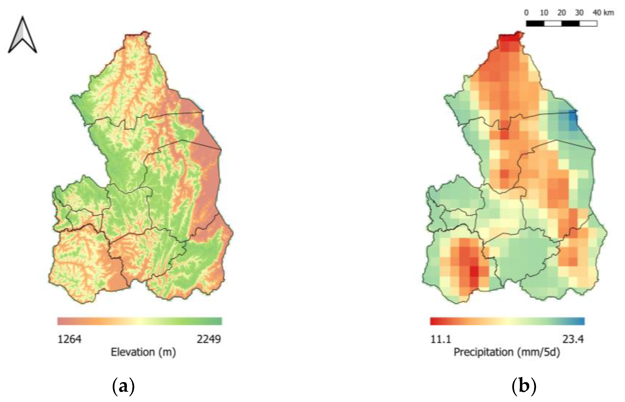
Located in the center of Africa, Rwanda is known for its multitude of different landscapes ranging from volcanoes and cloud forests to cropland and tropical savannah [42]. The topography of the study area is hilly, but not as mountainous as the western parts of the country. There is a gradient of higher elevation from the west to the east, with the eastern regions of the study area characterized by flat wetlands (Figure 2). The climate is highly seasonal and depends on precipitation patterns, with a long rainy season (late February–late May) followed by a long dry season (June–September) and a short rainy season (late September–early December) followed by a short dry season (mid-December–mid-February). The rainy seasons are responsible for determining the agricultural patterns and thus the livelihoods of the rural population [15].
Agricultural land in Rwanda makes up a total of 1.4 million ha (59% of total land area), of which 1 million ha are used for seasonal crops and the rest for perennial crops. The most common seasonal crops are maize, cassava, and beans, while the most common perennial crops are bananas, coffee, and tea. In the context of the study area, approximately 40% of the land area is under seasonal crop coverage and 29% is under perennial crop coverage [45]. As the majority of households own very small tracts of land, much of the cropland is used for subsistence agriculture, with a smaller proportion going toward export and foreign currency earning [42]. Furthermore, up to 40% of farmers practice agroforestry on their land, creating an important source of firewood and non-timber products as alternative income streams for the farming households [45]. This is particularly relevant in the Eastern Province, where agroforestry schemes can be found interspersed in cropland, creating a complex fabric of different land cover types.

2.2. Data Acquisition

All S2 images were acquired through GEE from the COPERNICUS/S2_SR collection. This is a publicly available collection of Level 2A (bottom-of-atmosphere corrected) products that can be filtered directly in GEE by both temporal and spatial bounds. Level 2A products were used because the processed products, after atmospheric correction to bottom-of-atmosphere reflectance, are more indicative of the actual spectral values seen at the vegetation level [46]. The area of interest for filtering was defined by the study area, and all tiles from both the dry season (1 June–30 September 2021) and the rainy season (1 February–30 May 2021) were further filtered by a maximum cloud cover percentage of 20 and 50 percent, respectively. Dry season months were used preferably because the lack of clouds gave a clearer, unobscured satellite image, but also because dry season months have been shown to produce more accurate results during the prediction of woody cover in tropical regions [47]. The rainy season images were acquired to allow for a comparison of the influence of seasonality on classification accuracy. However, due to the cloudy conditions during the rainy season, fewer images were available for processing and thus a higher cloud threshold was used. In total, 66 images were used from the dry season, and 46 images were used from the rainy season (Table 1). The settings for the rainy season were chosen to minimize the presence of cloud-masked artefacts; however, small cloud artefacts were still observed in some areas due to the seasonal weather and were masked to avoid impacts on the classification results.
In order to account for differences in land cover at different elevations, a non-spectral data source in the form of a 30 m resolution digital elevation model (DEM) obtained as part of the Shuttle Radar Topography Mission was also downloaded directly from the NASA dataset within GEE as an additional layer for classification [43]. The DEM was processed in GEE to calculate the slope angle, which was added as a separate layer (Figure 3a). As a representation of human settlements, population density data were obtained from Facebook Connectivity data [48]. These data show populated pixels in the study area obtained from mobile phone records, and from these data, a separate raster was calculated showing distance to populated areas (Figure 3b). This population raster was then normalized to obtain relative distance values and added as an additional layer for the classification algorithm.

2.3. Data Preparation and Inputs

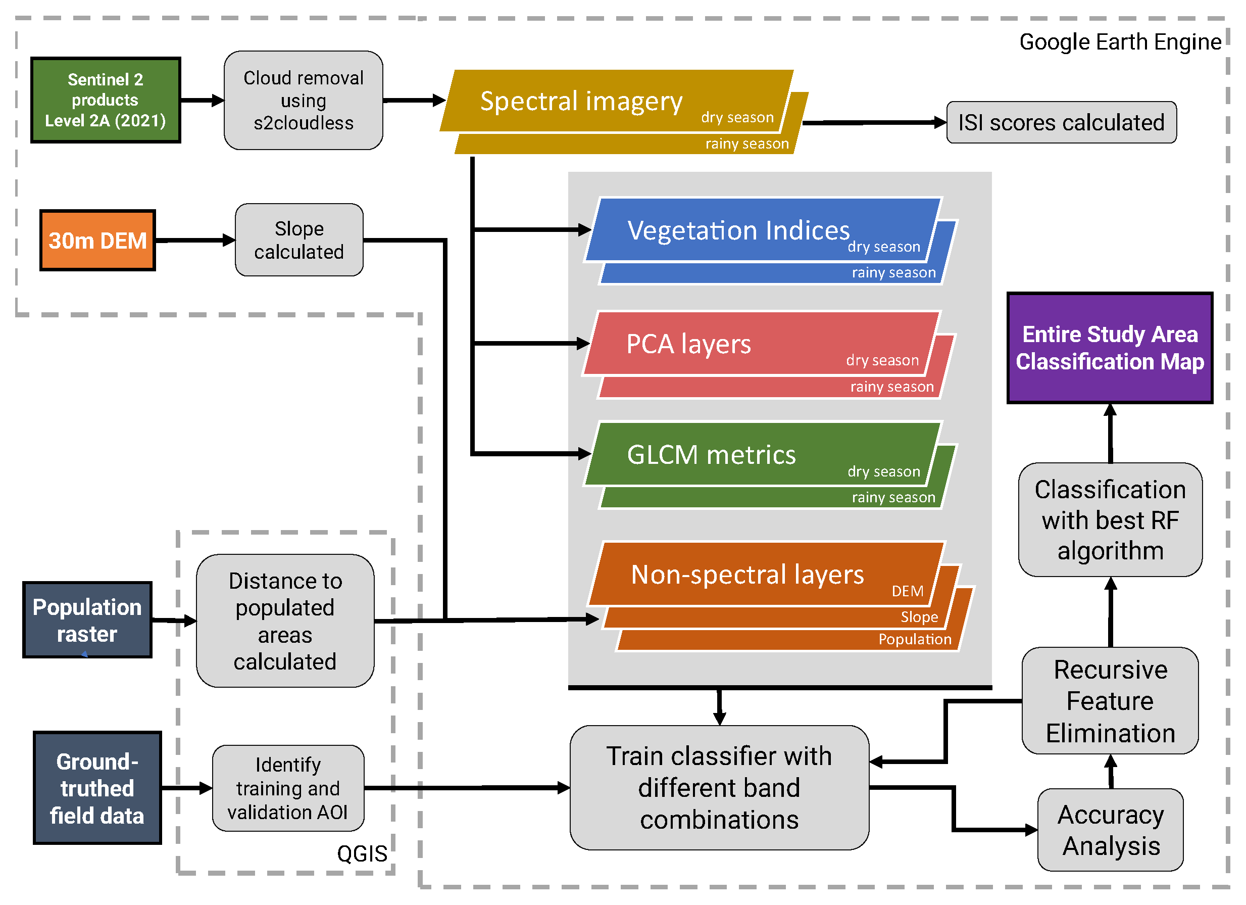
All acquired S2 images for both the rainy and dry season were processed using the s2cloudless algorithm in GEE to mask out clouds and cloud shadows. A cloud probability threshold of 30% was used, together with a maximum 1 km distance for cloud shadows and a buffer of 50 m to prevent cloud artefacts. Once clouds were removed from the images, they were stacked and a median value for each pixel was selected to represent the dry and rainy season stacked images. Median values were used to replace cloud-masked pixels with cloud-free pixels, where possible. The dry and rainy season median value images were each composed of 10 S2 bands: bands 2–8A (visible spectrum and near-infrared), 11, and 12 (shortwave infrared). The multiband median images were downloaded and used as inputs to the classification algorithm (Figure 4).
After the processing of the S2 images, eight additional vegetation indices were calculated for both the dry and rainy seasons using different combinations of the available spectral bands. These indices were chosen from a variety of similar studies in which they have been shown to increase classification accuracy and enhance the separation of similar classes (Table 2). Furthermore, in order to represent the texture of different land cover types in the classification algorithm, a gray level co-occurrence matrix (GLCM) was computed for each spectral band and season, with 7 texture metrics recorded across a 5 × 5 pixel window, for a total of 140 GLCM bands. GLCM texture metrics represent statistical measurements of the spatial relationship between pixel values within a window, and the specific metrics used in this study were selected as the most likely to be representative of different land cover types in previous classification studies [32,49,50]. Finally, a principal component analysis (PCA) was conducted on all spectral S2 bands for each season in order to capture the variability in spectral signals per season. The PCA analyses for each of the dry and rainy seasons resulted in 10 principal component layers (PC1-10), which were used as input data for the model. All indices, non-spectral layers, GLCM texture metrics, and PCA layers were used as inputs for the classification algorithm, for a total maximum of 199 possible input layers.
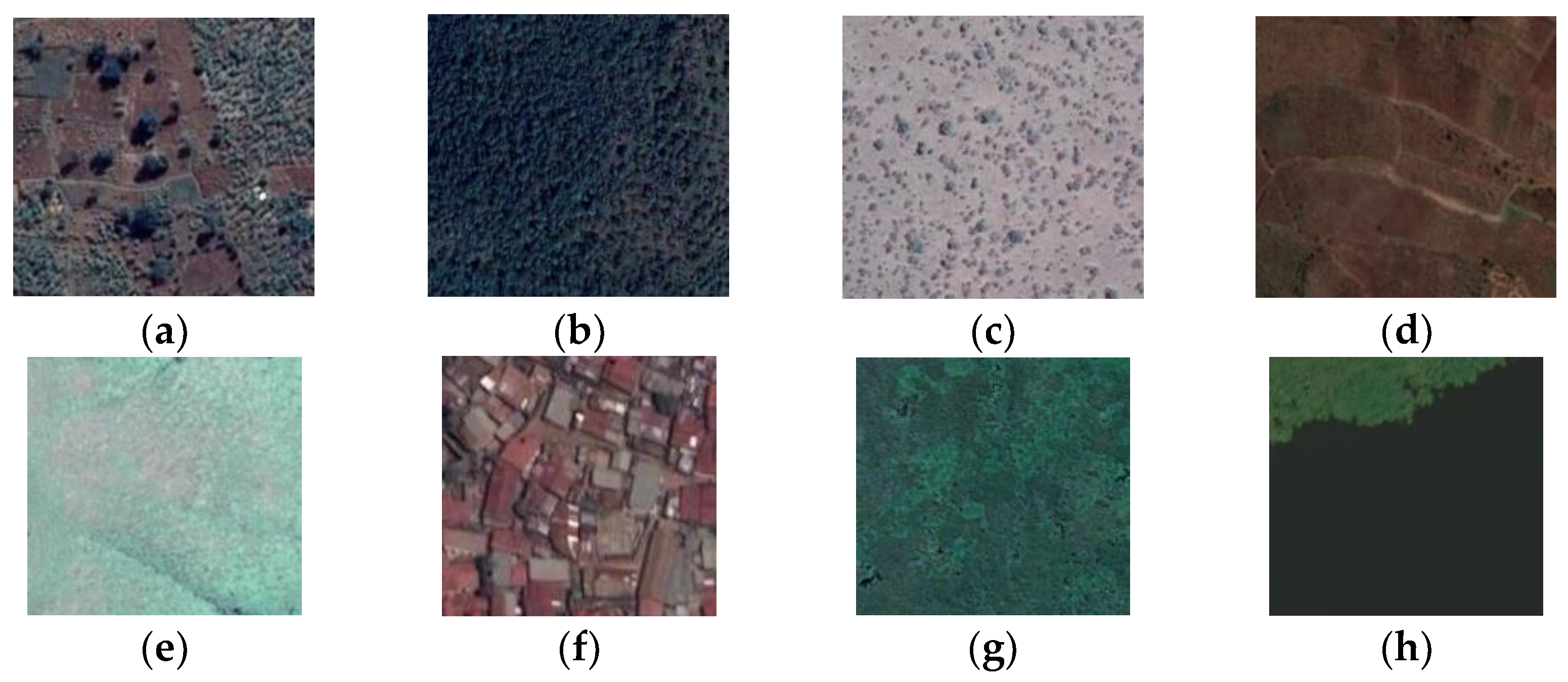
A clear and well-defined identification of the characteristics used to differentiate land cover types in a classification study should reduce confusion between classes during the classification process [53]. This has already been performed previously by government projects to classify land cover types in Rwanda which have generated a series of definitions based on different classes that contain trees and shrubs [54,55]. Using the past government studies as a foundation, a set of eight land cover classes was identified. Three of the land cover classes contain trees as integral parts of the land cover (forest, agroforestry, and shrublands) and were based on similar classes (trees in forest, trees outside forest on other land cover classes, and trees outside forest in shrubland) from specifications created in [55]. The other five classes were chosen to accurately cover and maximize differentiation between remaining land cover types (Figure 5).
Tree cover classes comprise the focal classes of this study. Trees in this study follow the definition from [55], which includes live trees, perennial shrubs, palms, and bamboo. The three tree cover classes in this study are thus defined as follows:
  • Agroforestry: trees in small woodlots (under 0.25 ha), trees growing in rows, and scattered trees on farms mixed with crops;
  • Forest: trees in natural forest or plantations with minimum 10% crown cover;
  • Shrubland: natural land cover with small shrubs (height under 7 m) and wooded savannah (height trees over 7 m) with minimum 10% crown cover.
Using the definitions above, a campaign to gather ground-truth point data for these classes was conducted in the study area between 1 August 2021 and 30 November 2021. For each sample point, data were collected on the GPS location as well as the type of tree cover. Upon analysis of the collected data, some points were removed due to errors in GPS measurement. The plot GPS locations were used as ground-truth training and validation data for their respective classes as an input for the classification algorithm. In total, 337 sample locations were used for the forest class, 182 sample locations for the agroforestry class, and 319 sample locations for the shrublands class.
The sample locations were visualized in QGIS 3.22.8, together with both median value images (from the dry and rainy seasons), as well as a Google Satellite layer. Each point location was individually checked to ensure the corresponding land cover type was correctly represented on all three imagery sources. Dry and rainy season S2 images were checked to ensure there were no cloud or mosaicking artefacts present in the imagery over each sample location. The S2 imagery was used to draw a polygon/region of interest (ROI) around each sample point encompassing the land cover type but not overlapping with other surrounding land cover types. The higher-resolution Google Satellite imagery, all of which was dated from 2020–2022, was used to verify that each ROI covered only the land cover type of interest, a method which has been beneficial for classification of medium-resolution imagery in past studies [26,27]. To prevent discrepancies in land cover at the acquisition date, ROI boundaries followed the land cover visible in the S2 imagery rather than in the Google Satellite imagery.
For land cover types not sampled as a part of the fieldwork campaign (cropland, grassland, urban, water, and wetland), the training data were assembled by identifying the appropriate land cover type on the Google Satellite imagery and selecting a polygon encompassing that land cover. For all polygons, a variety of different areas belonging to the same land cover type were selected to ensure model robustness and prevent overfitting. Each ROI identified was used as training data and paired with another polygon of similar size and similar area, covering the same land cover type, as validation data. Thus, two similar yet independent datasets were created for training and validation of the model accuracy. Of the ROIs identified, 50% were selected as training data, and 50% as test data for model accuracy assessment. Upon final assessment, the number of pixels used for the training and validation of each land cover type was at least 4000 pixels—significantly higher than the minimum ideal pixel number for accurate land cover classification of 500–1000 pixels per class as suggested by previous studies [36,37].

2.4. Spectral Separability of Classes

After identification of the ROIs for each class, the spectral values of each S2 band were assessed for separability between different classes. This was performed to create a statistical representation of the difference between the range of values present for each class and consider which band combinations may lead to a more accurate classification of the study area. The separability of the land cover classes was assessed using the instability index (ISI), which is a method of quantifying the variation between different endmember classes versus the natural spectral variation within each endmember class [56]. The definition of ISI is a simple ratio index calculated for each wavelength comparing the variation Δwithin,i to the variation Δbetween,i for two different endmember classes, calculated as:
I S I i = Δ w i t h i n , i Δ b e t w e e n , i = σ i , 1 + σ i , 2 x m e a n , i , 1     x m e a n , i , 2 ,
where 𝜎i,1, 𝜎i,2 represent the standard deviations and xmean,i,1, xmean,i,2 represent the mean reflectance values for classes 1 and 2, respectively [56]. Equation (1) was adapted to GEE and applied to the land cover classes in this study, with mean reflectance values and standard deviation calculated at each band wavelength individually rather than as a continuous variable across wavelengths.

2.5. Classification Algorithm

The classification algorithm used in this study was the RF algorithm, used directly in GEE as the ee.Classifier.smileRandomForest object. As a non-parametric machine learning model, RF is able to handle high dimensionality of inputs, using large numbers of decision trees to classify pixels according to their similarity to input training data. The authors of [25] conducted a review of S2 land cover classification studies, finding that the RF algorithm returned results with the highest accuracy scores, followed by the support vector machine algorithm. Furthermore, multiple other studies cited in this methodology also used RF as their classification algorithm [26,27,47]. The decision to use RF for this study was also upheld by a set of initial test calculations which determined RF to have higher accuracy compared to other GEE algorithms (CART and SVM).
The RF classifier was trained on the training ROI polygons using different combinations of the data available. Training layers included all available S2 spectral bands for both dry and rainy seasons, vegetation indices, GLCM texture metrics, PCA layers, and the non-spectral DEM, slope, and population layers. The trained classifier was then applied to the validation ROI polygons to derive accuracy statistics. An incremental addition of layers into the classification workflow was conducted in order to assess the change in classification accuracy with the addition of each new set of input layers. Kappa values, an accuracy metric that corrects for random chance of correct classification, were used in addition to overall accuracy to determine model accuracy. User’s and producer’s accuracy scores (UA and PA, respectively) and per-class F1 scores were used to determine model accuracy relative to each of the three tree cover classes. F1 scores were calculated per class using Equation (2) [33]:
F 1   =   2   ·   P A   ·   U A P A   +   U A ,
where PA and UA represent the producer’s accuracy and user’s accuracy for the class, respectively. The above accuracy metrics were calculated from confusion matrices generated in GEE for each model. From these confusion matrices, PA and UA scores were calculated per class, representing the probability of accurate classification and reliability of the classification, respectively. Overall accuracy was then calculated from all correct classifications (diagonals in the confusion matrix), and the Kappa value was used as a metric to correct for chance classification by incorporating all elements of a confusion matrix [57].

2.6. Feature Selection

As a part of its RF algorithm, GEE calculates variable importance (VI) scores for each input feature (in this case band layers) used in the classification. GEE uses a Gini impurity importance score, which is a sum of the reductions of impurity, or the probability of misclassification, by the feature in question at each split of a tree in an RF algorithm [58]. This method, though slightly less accurate than permutated importance measures, is faster and generally gives similar results [59]. The VI score represents the contribution of each feature (or layer) to increasing the classification accuracy scores, and thus to reducing impurity. VI scores were used for feature selection to reduce the number of input layers to the model. Feature selection was conducted manually using a recursive feature elimination method, where the feature with the lowest VI score was removed with each successive run of the model [33]. This process was repeated until all bands were removed in order to find the model with the highest accuracy, as well as the minimum number of input layers required to maintain a high accuracy.
Finally, in order to finetune the model and prevent overfitting of the model on the training data, three hyperparameters were tuned using a grid search approach, where the model was trained and validated with each combination of hyperparameters to find the most accurate combination. These hyperparameters were numberOfTrees, the number of decision trees in the model; bagFraction, the proportion of input data used in each iteration; and minLeafPopulation, the minimum training points used at each decision-making node. These hyperparameters and their default values were chosen according to previous studies investigating the impacts of hyperparameter tuning and feature selection on classification accuracy [33,34,60,61]. Once the best hyperparameters relative to the three tree cover classes had been identified, three models were selected to perform the final land cover classification of the study area: the model with the maximum number of input layers, the model with the highest accuracy, and the model with the minimum number of input layers required to maintain high accuracy. The classification results from these three models were then compared to assess similarities and differences in the results. All code used in GEE can be found in the Supplementary Materials.

3. Results

3.1. Spectral Separability

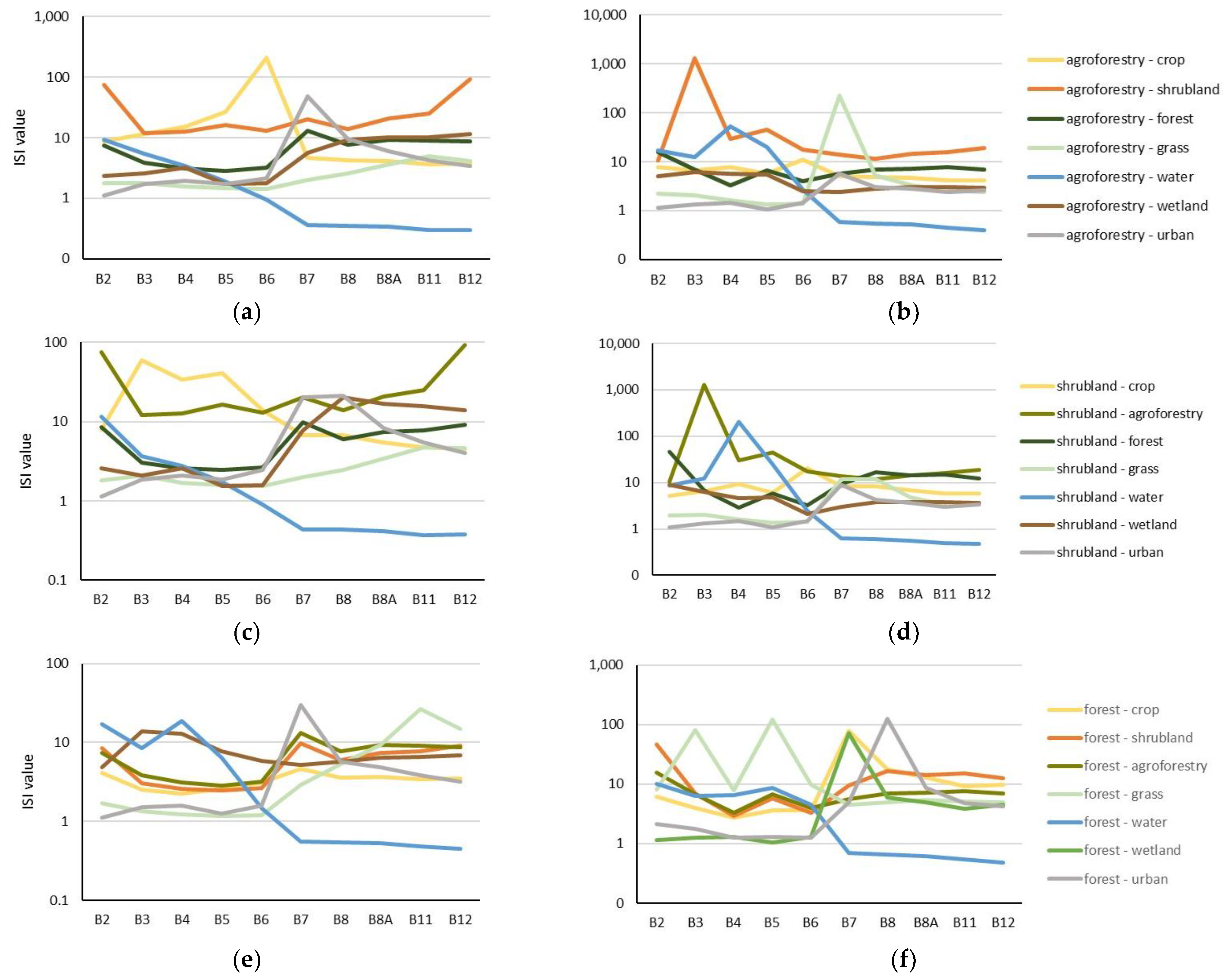
Spectral separability was assessed for both dry and rainy season median images using the ISI, in which values below 1 indicate a greater difference in spectral endmember signatures between assessed classes, while values above 1 indicate a greater difference in signatures within each class. The ISI values for the three tree cover classes were generally very high at each band when separability between each of these classes was assessed, indicating a very low separability between these classes using spectral bands alone. Notably, water was the single class that had ISI values below 1 for each of the tree cover classes (for bands 7, 8, 8A, 11, and 12) and thus a high separability from those classes using spectral bands alone. Dry season ISI values were lower for all band and land cover combinations than rainy season values (Figure 6).

3.2. Model Accuracy

A grid search approach was used to identify the combination of hyperparameters that would result in the highest accuracy for the final model. The GEE default combination for the model was 100 decision trees, a bagFraction value of 0.5, and a minLeafPopulation value of 1. However, the combination that yielded the highest accuracy was 500 decision trees, a bagFraction value of 0.25, and a minLeafPopulation value of 1. Generally, 500 decision trees resulted in the highest accuracies for any combination, while both increasing bagFraction and increasing minLeafPopulation resulted in lower overall accuracies (Table 3).
The RF algorithm was trained and validated on the same set of training and validation polygons for each band combination. All dry season bands were assessed first, with model M1 achieving F1 scores of 0.549 (agroforestry), 0.814 (forest), and 0.600 (shrubland; Table 4). Accuracy values were reduced when only rainy season bands were used to train and apply the RF algorithm (M2), and the combination of both dry and rainy season imagery (M3) yielded lower F1 scores than dry season imagery alone. Dry and rainy season vegetation indices also improved accuracy (M4), most notably for the shrubland class. The addition of PCA layers (M5) resulted in greatly improved F1 scores for all tree classes, especially agroforestry (improvement of over 5%) and forest (improvement of over 6%). Each non-spectral layer separately improved classification accuracy, yet with varying impacts on each tree class. Relative to model M5, the population layer (M6) had the highest improvement for the agroforestry F1 score (2%), the slope layer (M7) had the highest improvement for the forest F1 score (3%), and the DEM layer (M8) had the highest improvement for the shrubland F1 score (4%). The addition of all three non-spectral layers (M9) resulted in the highest F1 scores for the forest and shrubland classes. Finally, the combination of all bands in this study (199 total) was tested (model M10), resulting in higher F1 scores for both the agroforestry and shrubland classes, but a lower F1 score for the forest class. Both the overall accuracy and Kappa value were marginally higher for model M10 (88.2% and 86.8%) than for model M9 (87.2% and 85.4%).

3.3. Feature Selection

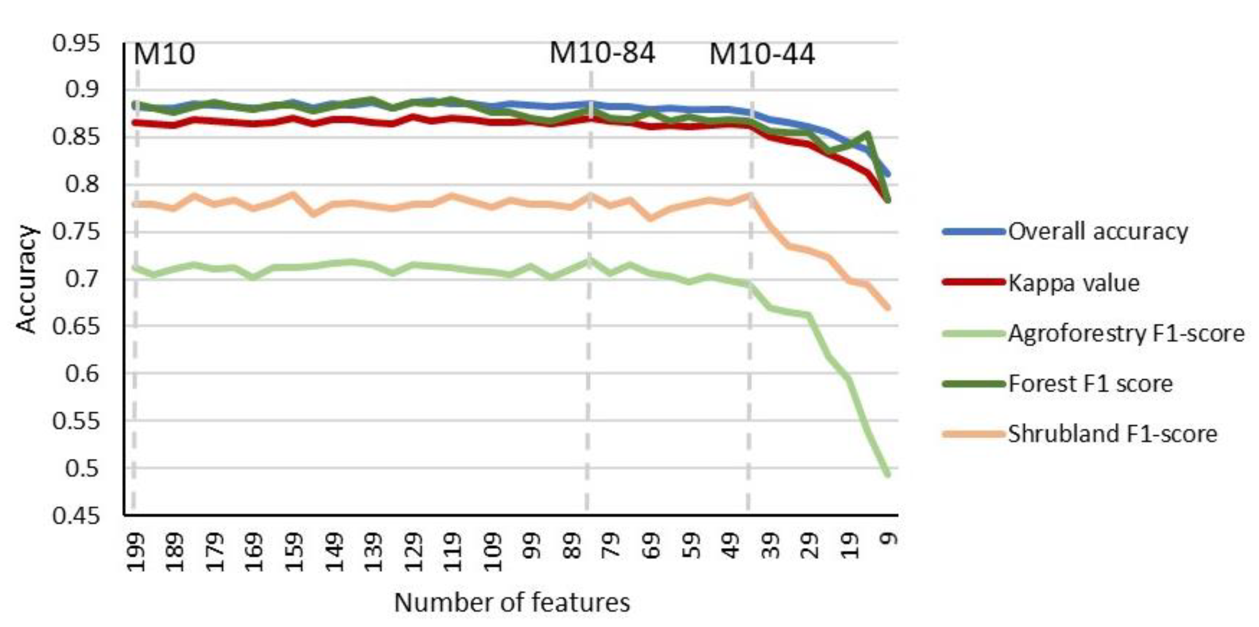
Feature selection was conducted using VI scores directly in GEE using the model with the maximum number of input layers (model M10) as the starting point. As least-important input layers were recursively eliminated, the model overall accuracy, model Kappa value, and F1 scores for each tree class remained stable until 44 input layers remained. At 44 input layers (model M10-44), an inflection point was reached, where the further removal of least-important input layers resulted in reduced model and tree class accuracies (Figure 7). The model with the highest overall accuracy and Kappa value, as well as the highest F1 scores for the agroforestry and shrubland classes, had a total of 84 input layers (model M10-84), which was less than half of the total potential input layers. The feature importances of all 84 layers of the best model were assessed in GEE through the calculated VI score.
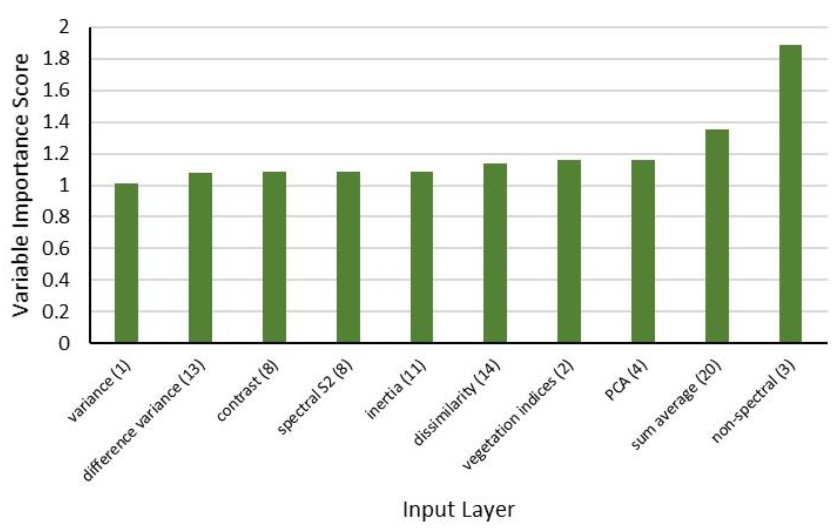
The three features with the highest importance were the non-spectral layers (slope, DEM, and population). In addition, notably high importance was given by the sum average layers of both rainy and dry season GLCMs for all spectral bands (Figure 8). Of the different GLCM texture metrics, inertia, difference variance, contrast, and dissimilarity were all selected as features for model M10-84, with average importance scores. Only a single variance band and none of the correlation bands were present in the final input features. Notably, most vegetation indices had been removed as low-importance features, with the exception of dry season NDWI and RGCI, which had average importance scores for this model. The remaining spectral S2 bands were B7 and B8A (dry season), and B5, B11, and B12 (both dry and rainy seasons). The remaining PCA layers were B3 and B6 (dry season), and B4 and B7 (rainy season). All remaining spectral S2 and PCA layers had low-to-average VI scores in this model, with the notable exception of the dry season spectral bands B11 and B12, and the rainy season PCA layer B7. Individual input layer VI scores can be found in the Supplementary Materials (Figure S1).
The accuracy metrics described above were also supported by confusion matrices describing the number of commonly confused pixels between each class. Table 5 shows the confusion matrix generated for model M10-84—the model which had the highest overall accuracy and Kappa value. All three tree cover classes have a high degree of confusion between each other. Agroforestry is most often misclassified as forest cover, followed by shrubland and crop cover. Forest is most often misclassified as agroforestry, followed by shrubland (to a lesser extent). Shrubland is most often misclassified as agroforestry, followed by cropland and grassland. While both agroforestry and shrubland are commonly misclassified as cropland, the forest class is not. Similarly, shrubland is more commonly confused for grassland than either agroforestry or forest.

3.4. Classification Maps

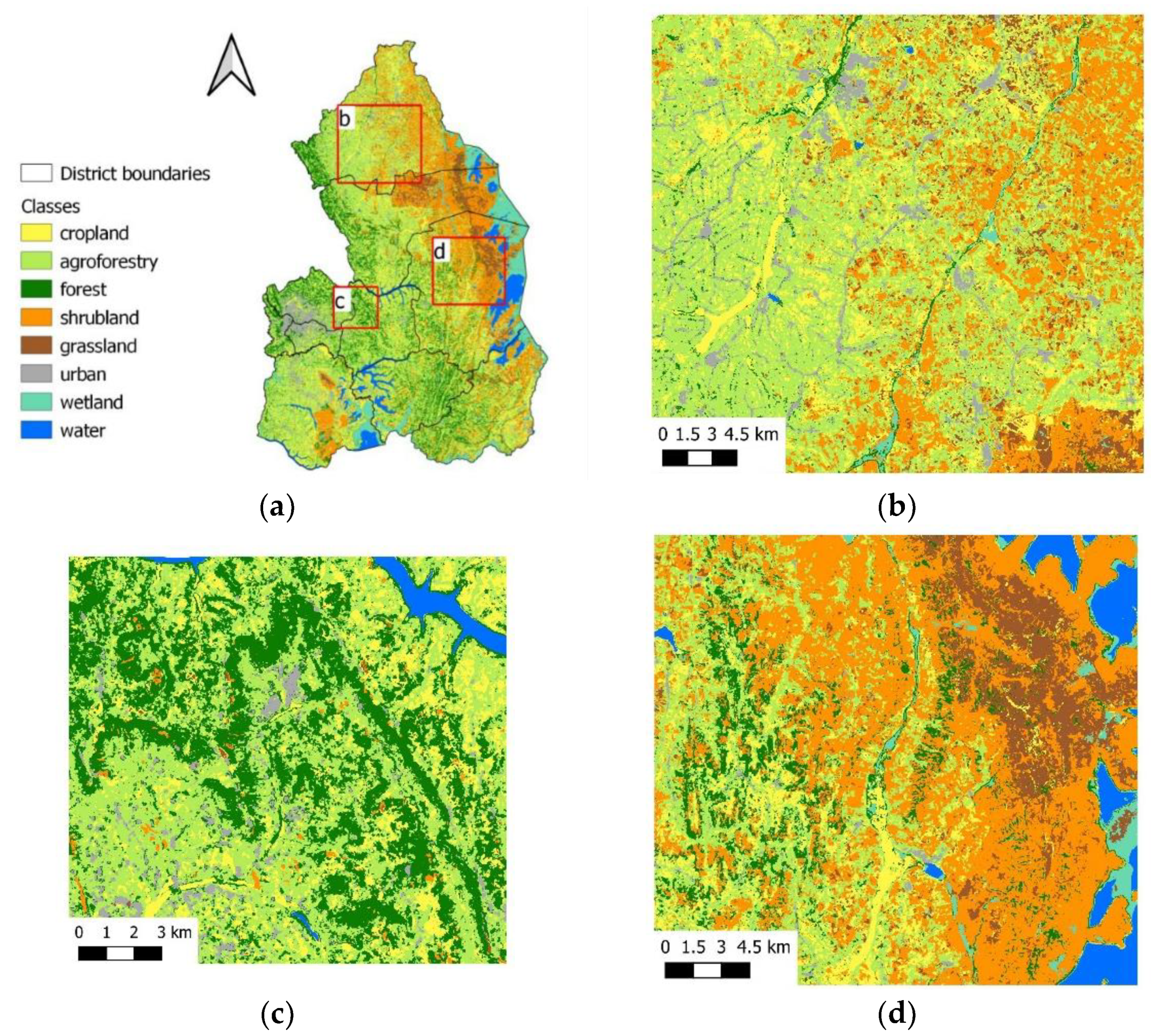
Three final classification maps were compared for patterns in land cover type delineation, and particularly for their effectiveness in delineating land cover types with trees. These were model M10: maximum number of input layers including both spectral imagery and PCA layers; model M10-84: the model with the highest accuracy scores according to the feature selection process; and model M10-44: the model with the least number of input features before reductions in accuracy. All three models predicted similar numbers of pixels in each tree class, with model M10-84 predicting the highest amount of forest cover, and an intermediate amount of agroforestry and shrubland cover relative to the other two models (Table 6). General patterns of land cover distribution across the study area were similar for all models, despite differences at local levels.
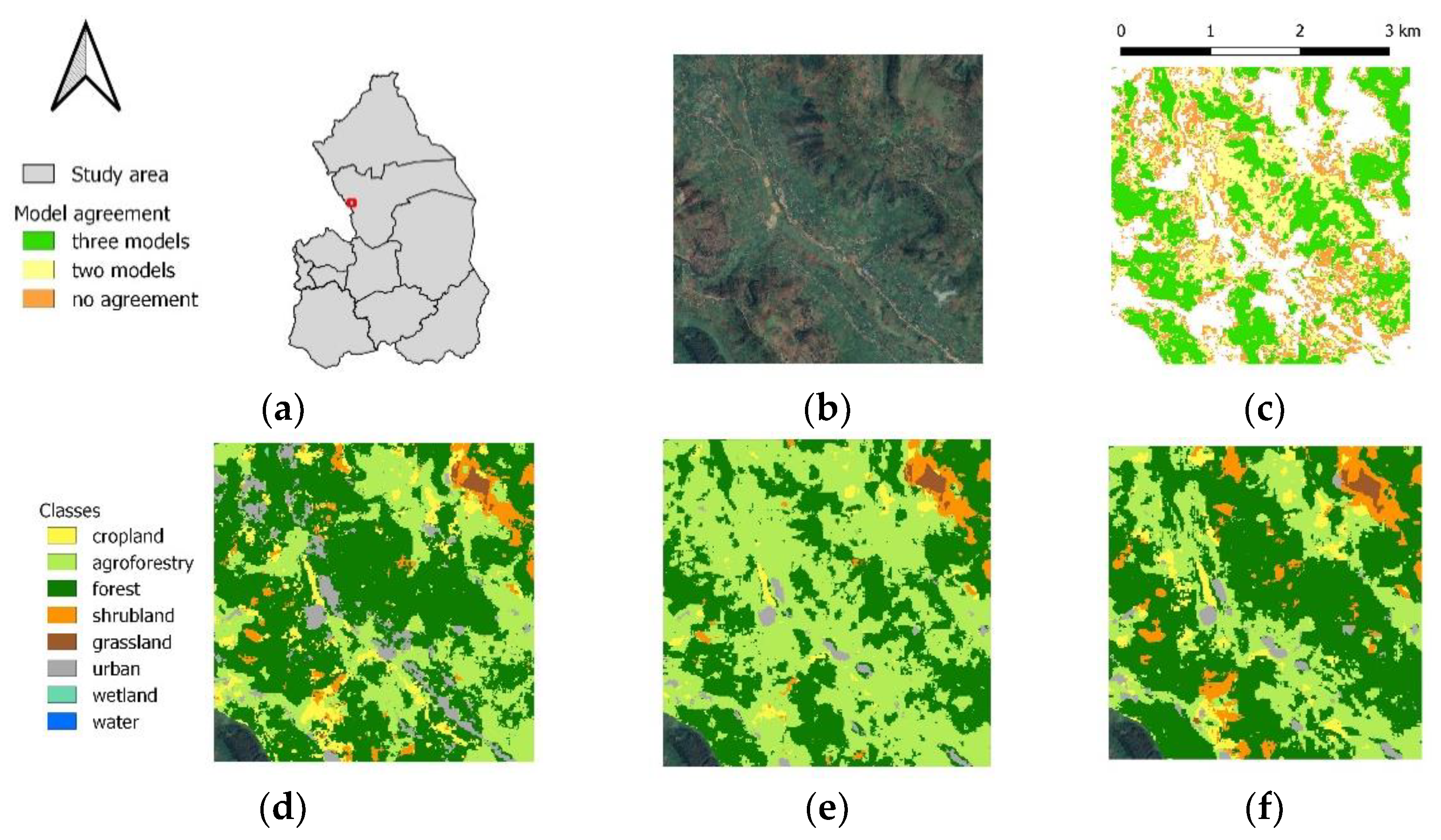
All three models described above predict similar patterns of forest cover, with model M10-84 predicting the largest total forest area. However, a visual check reveals that models M10 and M10-44 greatly overestimate forest cover in the study area (Figure 9). In contrast, model M10-84 shows more conservative predictions of forest cover, more clearly following visible patterns of actual cover. Model M10-84 predicts more small fragments of forest cover dispersed throughout the study area than either of the other models. Nonetheless, model M10-84 does still show some overestimations with regard to forest cover in some parts of the study area.
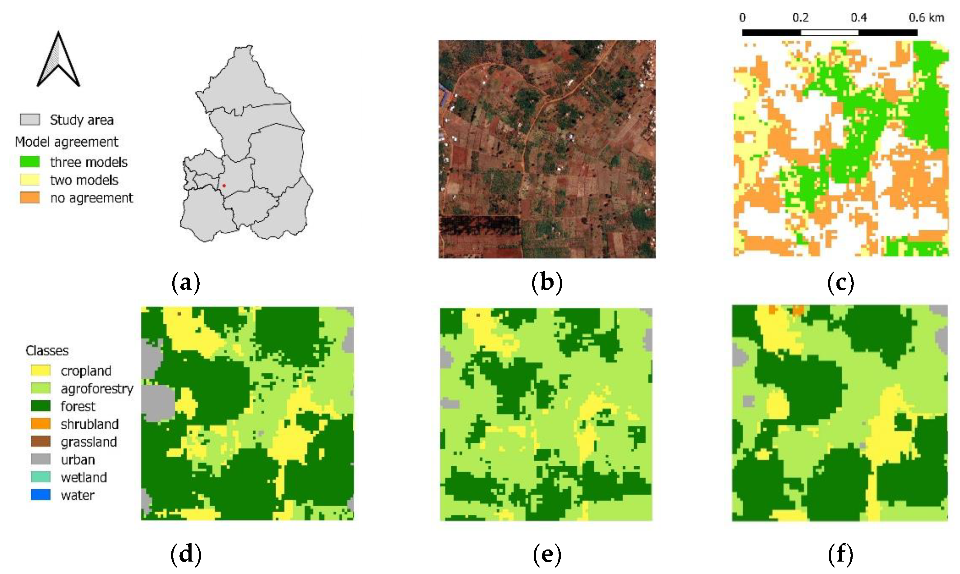
Agroforestry cover is generally well distributed throughout the study area, except for the more densely populated urbanized regions surrounding Kigali and the Akagera wetlands in the eastern regions of the study area. All models show similar distributions of agroforestry cover, although model M10-84 predicts more agroforestry in mountainous areas where both other models show larger areas of forest cover (Figure 10). In central regions of the study area, model M10-84 predicts less agroforestry than model M10, in favor of shrubland. However, this pattern continues as model M10-44 predicts even less agroforestry cover in this region, also in favor of shrubland.
Shrubland is distributed mainly in the eastern parts of the study area, as well as in the southcentral part of Bugesera district. In Bugesera, model M10-84 predicts more shrubland cover whereas model M10 predicts forest and agroforestry, while model M10-44 overestimates shrubland cover in this area. Around the eastern regions of the study area, model M10-84 predicts more shrubland rather than the cropland predicted by model M10 (Figure 11). In this same region, model M10-44 overestimates forest cover.
Pixel-based agreement on land cover type between the three models is generally high for all three tree cover classes, with the highest agreement for agroforestry and the lowest for forest. Of the total number of pixels classified as agroforestry by any of the models, 79% are classified as agroforestry by at least two models. From the total number of pixels classified as forest, 72% are classified as forest by at least two models. Finally, of the total number of pixels classified as shrubland, 75% are classified as such by at least two models. Model results can be found in the Supplementary Materials (Figures S5–S7).
Across the different districts in the study area, forest cover was largely concentrated on hillsides and the tops of hills (Figure 12c). Forest cover is mostly prevalent in the mountainous regions stretching from the northwestern to the southcentral part of the study area. Forest cover is especially high in Ngoma, Rwamagana, and Gasabo districts, as well as the westernmost parts of Nyagatare and Gatsibo districts. In the western parts of the study area, agroforestry is found in rural areas, in particular surrounding population centers and in the lowlands between forest cover on hills. In the eastern parts of the study area, agroforestry is found interspersed with shrubland and cropland, with a gradient of reducing agroforestry cover toward the arid easternmost parts of the country (Figure 12b). Shrublands are generally predicted on flat and lower elevation land in the study area, and especially in the more arid central/eastern regions (Figure 12d).

4. Discussion

4.1. Input Layers and Feature Selection

The spectral separability analysis conducted gave some insight into the challenges that would arise in the separation of tree cover classes in the study area. In particular, the ISI scores between all 3 tree cover classes (agroforestry, forest, shrubland) were higher than 1 for both the dry and rainy season spectral bands. This indicates a greater variability in band values within each class than between the separate classes [56]. The ISI scores for the rainy season were also notably higher for the rainy season bands than for the dry season bands, suggesting that dry season bands would be more suitable for the classification task. This is in agreement with [47], who similarly found that dry season bands were more suitable for monitoring woody cover dynamics using S2 imagery in tropical dry regions similar to the study area. The spectral separability analysis was confirmed during classification, where the input of dry season spectral bands alone resulted in higher accuracy rates for all three tree cover classes than either rainy or rainy and dry season bands. In line with this analysis, additional vegetation indices, non-spectral layers, and texture metrics further improved the classification results. This suggests that for such a dense and complex mosaic of land cover types, spectral imagery alone is insufficient for land cover classification because the S2 pixels consist of mixed spectral signals from similar types of vegetation and land cover. Nonetheless, the two SWIR bands (bands 11 and 12) had the highest feature importance scores of all the spectral bands, a finding suggesting their importance for tree cover classification and supported by the results of other studies [32,62].
Despite the improvement in classification accuracy with the addition of different input layers, there was clearly some redundancy in the inputs. This was evident from the relatively constant accuracy rates maintained during the feature selection process as least-important input layers were recursively eliminated from the RF inputs. However, there was also a clear benefit to this process, as model M10-84 was able to achieve higher accuracy rates and deliver more visually accurate predictions than the model that used all available input layers, model M10. Furthermore, there was a minimum number of input layers required to maintain model accuracy, defined as the model M10-44. This can be compared to [33], who were able to reduce the number of input features from 114 to 34 using a similar recursive elimination method. Similarly, other studies have shown that feature reduction is an effective method to reduce the number of RF input features, but that a minimum number of features remains necessary for accurate classification [63,64].
The elevation and topographic properties of the study area were key features for accurate land cover classification, as evidenced by the high feature importance scores of both the DEM and slope layers. This corresponds with the results of multiple studies, which show that elevation data are vital for separating forest and agroforestry classes, particularly in regions with a high variation in elevation and topography [32,65,66]. The importance of elevation in the study area may be rooted in the relationship between human populations and their surrounding landscapes. In the hilly regions of Gasabo, Nyagatare, and Gatsibo districts, the flat, low valley bottoms are mostly classified as cropland and agroforestry surrounding human settlements. These valleys are likely more fertile and have easier access to water resources, making them more well suited for agricultural land use. In contrast, the higher hilltops and sloped hillsides are classified as forest, which could be due to their relative inaccessibility, resulting in less pressure for deforestation through fuelwood gathering. This is supported by the high increase in forest classification accuracy with the addition of the slope layer in model M7. Such a relationship has been previously observed by [67], who found that slope degree was especially important for classifying wooded areas due to the difficulty of accessing those areas for agricultural purposes.
The population layer was also one of the most important features for each model, and its addition improved the F1 scores for all three tree classes, but especially for the agroforestry class. This improvement in agroforestry classification may be explained by the land use patterns of the rural populations. Past studies in Rwanda have underscored the importance of trees on farms and agroforestry systems for maintaining the livelihood of small-scale, rural farmers [14,68]. This is supported by visual assessment of the results, which show agroforestry in close proximity to human populations, particularly in rural areas, where the trees are integral for the provision of wood and non-timber products. The importance of non-spectral data to improving land cover classification accuracy supports the findings of [67], in which researchers similarly found greatly improved RF accuracy with the incorporation of open-access population and slope data. In such a densely populated country as Rwanda, which also has such a complex mosaic of land use, the addition of quantified social data, such as population distribution, can be a valuable method to map human impact on landscapes.
The addition of texture metrics similarly increased classification accuracy scores. In particular, the sum average GLCM metrics had the highest VI scores, and together with dissimilarity, difference variance, inertia, and contrast, were present in the input features of model M10-84, a finding which is supported by previous studies [32,69,70]. The author of [71] suggests that dissimilarity and contrast are key GLCM metrics to identify the edges of land cover patches, which would explain the importance of those features to classify the complex and fragmented land cover in the study area. The authors of [69] also used GLCM texture metrics in GEE to classify agroforestry and forest cover; however, they found that entropy and shade were also effective metrics to classify tree cover types. The authors of [35] found that GLCM metrics were particularly effective at identifying land cover with small patches of trees separated by large patches of bare soil or grass, such as the shrubland class in this study. The improvements in classification accuracy as a result of model training with GLCM metrics underscore their importance for classification in mosaic landscapes. This is likely due to the metrics describing the local regions around each pixel, allowing the input data to capture the inherent complexity of such fragmented landscapes.
The results of the feature selection process demonstrated that vegetation indices were not of a high importance for land cover classification in this study. Only two dry season vegetation indices, NDWI and RGCI, remained as input layers for model M10-84, suggesting that the differences in vegetation described by these indices were sufficiently covered by the more important input layers, such as the remaining GLCM layers. Similarly, only four PCA layers (PC6, PC2, PC5, and PC3) remained in model M10-84, suggesting that these were the principal components that best explained the remaining variability between the different land cover classes. This finding suggests that the feature selection process allowed the removal of spectral and PCA layers that were redundant, leaving the model to use only those layers that most effectively contributed to increasing classification accuracy. Furthermore, the feature selection process suggests that the exclusion of layers from processing in such a study should not be conducted a priori, but rather through a feature elimination process as conducted here. Though this may not decrease the amount of input data for the model, it is still beneficial for both improving accuracy and the processing time.

4.2. Tree Cover Class Distribution

The distribution of both the shrubland and agroforestry classes follows a steady eastward gradient, as human populations thin out and shrublands become more common. This pattern is similar to that described by [72], who describe the growing encroachment of cropland and agroforestry on the arid eastern shrublands due to the post-genocide resettlement of refugees and the expansion of cattle grazing lands and agropastoralism in the region. The degradation of shrubland cover to crop- and grassland in this region may decrease the availability of woody biomass for local populations, potentially leading to challenges for both the populations and local government in promoting sustainable firewood usage. The high population density of Rwanda and the limitations in space for both agriculture and forestry mean that there is not enough land in the study area for reforestation on a large scale. Current government schemes to integrate more trees into the agricultural landscape are thus a logical choice, with efforts applied to promote agroforestry as a solution to decrease deforestation and improve firewood provision for rural populations [7]. Until now, the regular and continuous monitoring of agroforestry cover was prohibitively expensive, as it required expensive fieldwork or very high-resolution imagery (expensive to acquire). Imagery was either interpreted in a visual way (thus introducing a subjective element), or required applying deep learning methods on imagery that are difficult to obtain on a regular basis [24,54]. This study demonstrates that a more objective digital method using publicly available S2 imagery can deliver reliable results with much less expense. The methods presented in this study thus give policymakers and researchers the tools to allow for monitoring and detecting changes in agroforestry, as well as forest and shrubland cover, in a qualitative and cost-effective manner. Such monitoring can support government efforts to integrate trees into the landscape, and to maximize the effective use of land in such a densely populated region [54].

4.3. Comparison to Other Studies

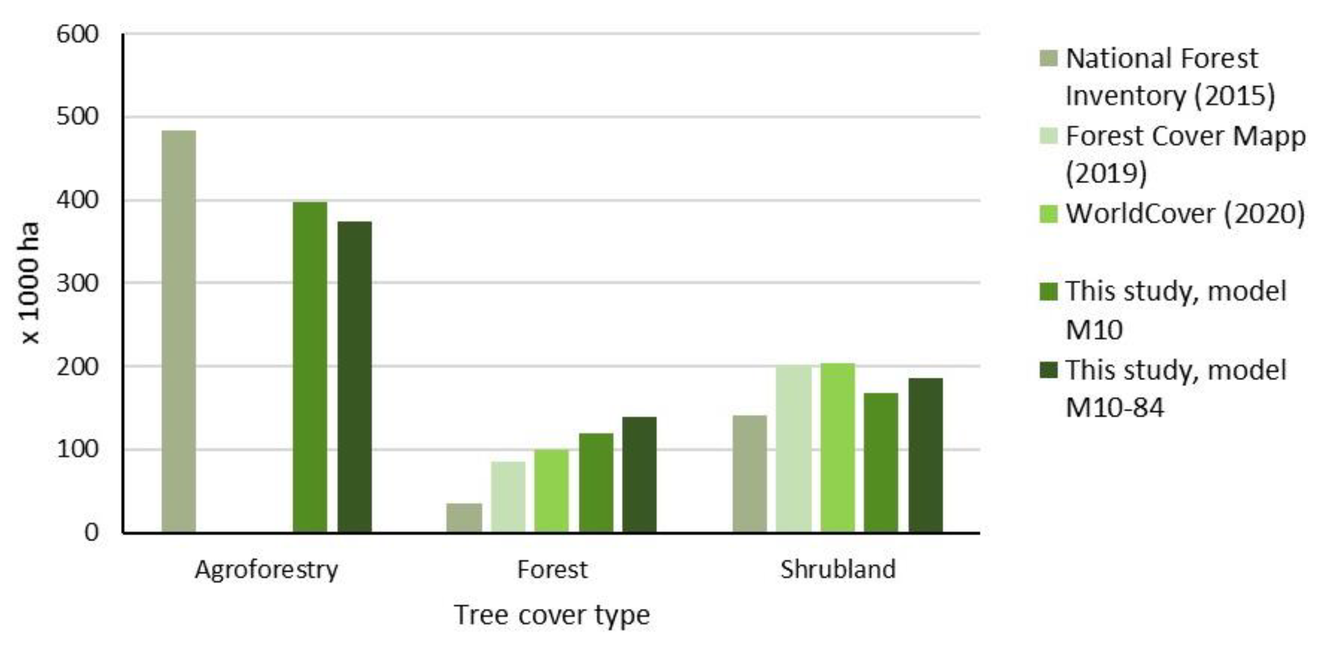
Compared to past research conducted during the forest cover mapping study (FCM) in 2019, this study has identified 41% more forest cover with model M10, which utilized all input layers, and 64% more forest cover with model M10-84, the model with the highest accuracy [54]. The pattern is reversed for shrubland cover, where this study identified 18% less shrubland with model M10, and 9% less shrubland cover with model M10-84. The FCM did not assess agroforestry cover. Spatially, the patterns of forest and shrubland cover distribution predicted in this study closely match the distribution of forest and shrubland in the FCM report (Figures S2 and S3). The 2015 National Forest Inventory (NFI) used a previous forest cover map from 2009, as well as limited remote sensing methods and vast fieldwork efforts to study tree cover in Rwanda [55]. The models trained in this study predicted generally similar total areas for both the agroforestry and shrubland classes (Figure 13). Model M10 predicted 17% less agroforestry than was reported in the NFI and 19% more shrubland. However, model M10-84 predicted 23% less agroforestry cover and 32% more shrubland. The total forest area predicted in this study by each of the two models was three to four times higher than that identified in the NFI. This can partly be attributed to the fact that the NFI did not consider woodlots under 0.25 ha in size as ‘forest’, while this study classified them as such due to the absence of size limitations. Because the NFI was also based on a forest cover map from 2009, the forest cover discrepancies could also reflect reforestation efforts in the study area over the past twelve years. Furthermore, as described in the NFI, mature and productive forests were counted as forest cover, while young forests were not counted. In light of the many government reforestation initiatives since the NFI was last conducted, this further suggests some of the differences could be due to forests that were not considered in the NFI, but which can nonetheless be seen from satellite imagery. The differences in tree cover area between the different studies further underscore the difficulty of accurately classifying mosaic landscapes, as the classes are often fragmented and mixed with other classes in reality.
Finally, the results of this study were also compared with the 10 m WorldCover product, a similar land cover classification product with global coverage [73]. WorldCover does not have an agroforestry class, but it was possible to compare both the forest and shrubland classes. Model M10 predicted 21% more forest cover and 18% less shrubland cover than the WorldCover product. In contrast, model M10-84 predicted 40% more forest cover and only 9% less shrubland cover than the WorldCover product. As WorldCover is a similar land cover classification product, this comparison is promising, showing that by using a much smaller local training dataset it is still possible to obtain similar results. Despite the overestimation of forest cover by models in this study, model M10-84 also correctly identified areas of forest that are not identified as such in neither the FCM nor WorldCover (Figure S4). The overestimation of forest cover in model M10-84 is most notable in regions of low-density forest, which is a challenge directly opposite to that faced by [24], who encountered challenges with identifying dense forest in the study area. This suggests that a fusion approach could be beneficial for future research: combining RF classification for dense forest and deep learning methods for open forest areas.
Some of the discrepancies between results obtained in this study and those reported in other studies may also be due to limitations in both the methodology and the data used in this study. The choice of Facebook Connectivity data as a source for the delineation of population was made as it is the highest resolution and most recent dataset available but may have biased the results by showing mostly populations with access to mobile phones, reducing the apparent impact of those people that may not have access to such devices. Because the purpose was to use publicly available Sentinel imagery with a maximum resolution of 10 m, many of the pixels in the study area consisted of mixed spectral signals from the fragmented and intermixed land cover types. Particularly for the agroforestry and shrubland classes, this may have caused some of the confusion with similar classes (cropland and grassland, respectively). The authors of [74] developed an approach to unmix Sentinel spectral signals and reduce classification error; however, this approach has not been applied here. Furthermore, the use of GEE as a processing tool enabled the use of large amounts of data and processing resources; however, it limited the availability of machine learning algorithms to those already available in GEE. Next generation methods such as artificial neural networks and deep learning algorithms show promising results for land cover classification, and could be a viable alternative for future studies [75,76,77].

5. Conclusions

The complexity of mosaic landscapes in Rwanda poses a serious challenge for land cover classification, and particularly for the accurate identification and separation of land cover classes containing trees. The high spectral similarity between different land cover types suggests that the use of spectral imagery alone is not enough for accurate classification. Such a similarity requires the use of additional layers such as vegetation indices, texture metrics, principal component analysis bands, and non-spectral datasets. Once these additional layers are included for training, machine learning classification using random forests can generate accurate results over a large study area. Furthermore, a robust feature selection process can help to remove redundant features and identify the most important features for future classification. Result accuracy is, however, dependent on the land cover type, with forest, a more clearly defined and less spectrally mixed class, reaching higher accuracy scores than agroforestry or shrubland, both of which are spectrally mixed classes that can at times be difficult to separate from other classes. This study provides an alternative method of classifying tree cover in Rwanda, using freely available medium-resolution imagery that complements existing research using expensive high-resolution imagery and extensive but costly fieldwork. In contrast, the fieldwork required for the methods presented in this study are limited in both time and cost, allowing for classification results over a larger area with less intensive sampling. The methods demonstrated in this study, combined with periodic, but limited, fieldwork to generate ground-truth training and validation data, can help provide continuous monitoring of land cover types containing trees in the study area. Such continued monitoring could be especially beneficial to the agroforestry sector in the country, helping to support government initiatives to ensure the sustainable use of tree resources.

Supplementary Materials

The following supporting information can be downloaded at: https://www.mdpi.com/article/10.3390/rs15102606/s1, Figure S1: individual input layer variable importance ranking; Figure S2: forest cover comparison; Figure S3: shrubland cover comparison; Figure S4: forest cover not identified in other studies; Figure S5: classification map of three northernmost Eastern Province districts; Figure S6: classification map of four southernmost Eastern Province districts; Figure S7: classification map of three Kigali City districts; all code files.

Author Contributions

Conceptualization, N.G. and V.U.; methodology, N.G., V.U. and B.V. software, N.G.; validation, N.G., V.U., B.V. and B.S.; formal analysis, N.G.; investigation, N.G. and V.U.; writing—original draft preparation, N.G., V.U. and B.V.; writing—review and editing, N.G., V.U., B.V., B.S. and B.M.; visualization, N.G.; supervision, B.V., V.U. and B.S.; project administration, B.V.; funding acquisition, B.V. All authors have read and agreed to the published version of the manuscript.

Funding

This research was funded by the European Union through the “Development of Smart Innovation through Research in Agriculture (DeSiRa)” grant (RWA/8000 DeSiRa, EU CA—FOOD/2019/412/627).

Data Availability Statement

Data and information can be obtained upon request by contacting the authors ([email protected] and [email protected]).

Acknowledgments

The authors would like to thank the Ministry of Environment of Rwanda for providing training data, ENABEL for providing data and their support during fieldwork, and ICRAF for additional data. We also thank KU Leuven and VITO for supervision and guidance during the development and completion of this study.

Conflicts of Interest

The authors declare no conflict of interest.

References

  1. Keenan, R.J.; Reams, G.A.; Achard, F.; de Freitas, J.V.; Grainger, A.; Lindquist, E. Dynamics of Global Forest Area: Results from the FAO Global Forest Resources Assessment 2015. For. Ecol. Manag. 2015, 352, 9–20. [Google Scholar] [CrossRef]
  2. Curtis, P.G.; Slay, C.M.; Harris, N.L.; Tyukavina, A.; Hansen, M.C. Classifying Drivers of Global Forest Loss. Science 2018, 361, 1108–1111. [Google Scholar] [CrossRef] [PubMed]
  3. Williams, B.A.; Venter, O.; Allan, J.R.; Atkinson, S.C.; Rehbein, J.A.; Ward, M.; Marco, M.D.; Grantham, H.S.; Ervin, J.; Goetz, S.J.; et al. Change in Terrestrial Human Footprint Drives Continued Loss of Intact Ecosystems. One Earth 2020, 3, 371–382. [Google Scholar] [CrossRef]
  4. Hosonuma, N.; Herold, M.; Sy, V.D.; Fries, R.S.D.; Brockhaus, M.; Verchot, L.; Angelsen, A.; Romijn, E. An Assessment of Deforestation and Forest Degradation Drivers in Developing Countries. Environ. Res. Lett. 2012, 7, 044009. [Google Scholar] [CrossRef]
  5. Nishimwe, G.; Rugema, D.M.; Uwera, C.; Graveland, C.; Stage, J.; Munyawera, S.; Ngabirame, G. Natural Capital Accounting for Land in Rwanda. Sustainability 2020, 12, 5070. [Google Scholar] [CrossRef]
  6. Ndoli, A.; Mukuralinda, A.; Schut, A.G.T.; Iiyama, M.; Ndayambaje, J.D.; Mowo, J.G.; Giller, K.E.; Baudron, F. On-Farm Trees Are a Safety Net for the Poorest Households Rather than a Major Contributor to Food Security in Rwanda. Food Secur. 2021, 13, 685–699. [Google Scholar] [CrossRef]
  7. Ministry of Lands and Forestry. Rwanda National Forestry Policy 2018; Ministry of Lands and Forestry: Kigali, Rwanda, 2018.
  8. Cooper, M.; Zvoleff, A.; Gonzalez-Roglich, M.; Tusiime, F.; Musumba, M.; Noon, M.; Alele, P.; Nyiratuza, M. Geographic Factors Predict Wild Food and Nonfood NTFP Collection by Households across Four African Countries. For. Policy Econ. 2018, 96, 38–53. [Google Scholar] [CrossRef]
  9. Mutandwa, E.; Kanyarukiga, R. Understanding the Role of Forests in Rural Household Economies: Experiences from the Northern and Western Provinces of Rwanda. South. For. A J. For. Sci. 2016, 78, 115–122. [Google Scholar] [CrossRef]
  10. Nahayo, A.; Ekise, I.; Niyigena, D. Assessment of the Contribution of Non Timber Forest Products to the Improvement of Local People’s Livelihood in Kinigi Sector, Musanze District, Rwanda. Ethiop. J. Environ. Stud. Manag. 2013, 6, 698–706. [Google Scholar] [CrossRef]
  11. Rurangwa, F.; Kinyanjui, M.J.; Bazimaziki, F.; Peeters, J.; Munyehirwe, A.; Musoke, F.; Habiyaremye, G.N.; Bakundukize, D.; Ngabonziza, P.; Uwase, J. Developing a Forest Management Plan (DFMP) for Gatsibo District in the Eastern Province of Rwanda. Open J. For. 2018, 8, 247. [Google Scholar] [CrossRef]
  12. Kiyani, P.; Andoh, J.; Lee, Y.; Koo Lee, D. Forest Science and Technology Benefits and Challenges of Agroforestry Adoption: A Case of Musebeya Sector, Nyamagabe District in Southern Province of Rwanda Benefits and Challenges of Agroforestry Adoption: A Case of Musebeya Sector, Nyamagabe District in Southern Province of Rwanda. For. Sci. Technol. 2017, 13, 174–180. [Google Scholar] [CrossRef]
  13. Iiyama, M.; Mukuralinda, A.; Ndayambaje, J.; Musana, B.; Ndoli, A.; Mowo, J.; Garrity, D.; Ling, S.; Ruganzu, V. Tree-Based Ecosystem Approaches (TBEAs) as Multi-Functional Land Management Strategies—Evidence from Rwanda. Sustainability 2018, 10, 1360. [Google Scholar] [CrossRef]
  14. Ndayambaje, J.D.; Mugiraneza, T.; Mohren, G.M.J. Woody Biomass on Farms and in the Landscapes of Rwanda. Agrofor. Syst. 2014, 88, 101–124. [Google Scholar] [CrossRef]
  15. Ndayisaba, F.; Guo, H.; Bao, A.; Guo, H.; Karamage, F.; Kayiranga, A. Understanding the Spatial Temporal Vegetation Dynamics in Rwanda. Remote Sens. 2016, 8, 129. [Google Scholar] [CrossRef]
  16. Bagstad, K.J.; Ingram, J.C.; Lange, G.-M.; Masozera, M.; Ancona, Z.H.; Bana, M.; Kagabo, D.; Musana, B.; Nabahungu, N.L.; Rukundo, E.; et al. Towards Ecosystem Accounts for Rwanda: Tracking 25 Years of Change in Flows and Potential Supply of Ecosystem Services. People Nat. 2020, 2, 163–188. [Google Scholar] [CrossRef]
  17. Ndayambaje, J.D.; Mohren, G.M.J. Fuelwood Demand and Supply in Rwanda and the Role of Agroforestry. Agrofor. Syst. 2011, 83, 303–320. [Google Scholar] [CrossRef]
  18. Drigo, R.; Munyehirwe, A.; Nzabanita, V.; Munyampundu, A. Rwanda Supply Master Plan for Fuelwood and Charcoal; Ministry of Natural Resources: Kigali, Rwanda, 2013. [Google Scholar]
  19. Akinyemi, F.O. Land Change in the Central Albertine Rift: Insights from Analysis and Mapping of Land Use-Land Cover Change in North-Western Rwanda. Appl. Geogr. 2017, 87, 127–138. [Google Scholar] [CrossRef]
  20. Basnet, B.; Vodacek, A. Monitoring the Dynamics of Land Cover in the Lake Kivu Region Using Multi-Temporal Landsat Imagery. In Proceedings of the 2014 IEEE Geoscience and Remote Sensing Symposium, Quebec City, QC, Canada, 13–18 July 2014; pp. 4250–4253. [Google Scholar]
  21. Hawinkel, P. Modeling Vegetation Dynamics Driven by Climate Variability and Lan. Ph.D. Thesis, KU Leuven, Leuven, Belgium, 2019. [Google Scholar]
  22. Mugiraneza, T.; Haas, J.; Ban, Y. Spatiotemporal Analysis of Urban Land Cover Changes in Kigali, Rwanda Using Multitemporal Landsat Data and Landscape Metrics. In Proceedings of the International Archives of the Photogrammetry, Remote Sensing and Spatial Information Sciences—ISPRS Archives, Tshwane, South Africa, 8–12 May 2017; pp. 137–144. [Google Scholar]
  23. Mugiraneza, T.; Nascetti, A.; Ban, Y. Continuous Monitoring of Urban Land Cover Change Trajectories with Landsat Time Series and Landtrendr-Google Earth Engine Cloud Computing. Remote Sens. 2020, 12, 2883. [Google Scholar] [CrossRef]
  24. Mugabowindekwe, M.; Brandt, M.; Chave, J.; Reiner, F.; Skole, D.L.; Kariryaa, A.; Igel, C.; Hiernaux, P.; Ciais, P.; Mertz, O.; et al. Nation-Wide Mapping of Tree-Level Aboveground Carbon Stocks in Rwanda. Nat. Clim. Chang. 2023, 13, 91–97. [Google Scholar] [CrossRef]
  25. Phiri, D.; Simwanda, M.; Salekin, S.; Nyirenda, V.R.; Murayama, Y.; Ranagalage, M. Sentinel-2 Data for Land Cover/Use Mapping: A Review. Remote Sens. 2020, 12, 2291. [Google Scholar] [CrossRef]
  26. Li, W.; Buitenwerf, R.; Munk, M.; Bøcher, P.K.; Svenning, J.-C. Deep-Learning Based High-Resolution Mapping Shows Woody Vegetation Densification in Greater Maasai Mara Ecosystem. Remote Sens. Environ. 2020, 247, 111953. [Google Scholar] [CrossRef]
  27. Nomura, K.; Mitchard, E. More Than Meets the Eye: Using Sentinel-2 to Map Small Plantations in Complex Forest Landscapes. Remote Sens. 2018, 10, 1693. [Google Scholar] [CrossRef]
  28. Ouattara, B.; Forkuor, G.; Zoungrana, B.J.B.; Dimobe, K.; Danumah, J.; Saley, B.; Tondoh, J.E. Crops Monitoring and Yield Estimation Using Sentinel Products in Semi-Arid Smallholder Irrigation Schemes. Int. J. Remote Sens. 2020, 41, 6527–6549. [Google Scholar] [CrossRef]
  29. Van Der Meer, F.; Bakker, W.; Scholte, K.; Skidmore, A.; De Jong, S.; Clevers, J.; Addink, E.; Epema, G. Spatial Scale Variations in Vegetation Indices and Above-Ground Biomass Estimates: Implications for MERIS. Int. J. Remote Sens. 2001, 22, 3381–3396. [Google Scholar] [CrossRef]
  30. Rahman Sarker, L.; Nichol, J.E. Improved Forest Biomass Estimates Using ALOS AVNIR-2 Texture Indices. Remote Sens. Environ. 2011, 115, 968–977. [Google Scholar] [CrossRef]
  31. Ghebrezgabher, M.G.; Yang, T.; Yang, X.; Wang, X.; Khan, M. Extracting and Analyzing Forest and Woodland Cover Change in Eritrea Based on Landsat Data Using Supervised Classification. Egypt. J. Remote Sens. Space Sci. 2016, 19, 37–47. [Google Scholar] [CrossRef]
  32. Nandasena, W.D.K.V.; Brabyn, L.; Serrao-Neumann, S. Using Google Earth Engine to Classify Unique Forest and Agroforest Classes Using a Mix of Sentinel 2a Spectral Data and Topographical Features: A Sri Lanka Case Study. Geocarto Int. 2021, 37, 9544–9559. [Google Scholar] [CrossRef]
  33. Dobrinić, D.; Gašparović, M.; Medak, D. Evaluation of Feature Selection Methods for Vegetation Mapping Using Multitemporal Sentinel Imagery. Int. Arch. Photogramm. Remote Sens. Spat. Inf. Sci. 2022, XLIII-B3-2022, 485–491. [Google Scholar] [CrossRef]
  34. Stromann, O.; Nascetti, A.; Yousif, O.; Ban, Y. Dimensionality Reduction and Feature Selection for Object-Based Land Cover Classification Based on Sentinel-1 and Sentinel-2 Time Series Using Google Earth Engine. Remote Sens. 2020, 12, 76. [Google Scholar] [CrossRef]
  35. Rodriguez-Galiano, V.F.; Ghimire, B.; Rogan, J.; Chica-Olmo, M.; Rigol-Sanchez, J.P. An Assessment of the Effectiveness of a Random Forest Classifier for Land-Cover Classification. ISPRS J. Photogramm. Remote Sens. 2012, 67, 93–104. [Google Scholar] [CrossRef]
  36. Thanh Noi, P.; Kappas, M. Comparison of Random Forest, k-Nearest Neighbor, and Support Vector Machine Classifiers for Land Cover Classification Using Sentinel-2 Imagery. Sensors 2018, 18, 18. [Google Scholar] [CrossRef] [PubMed]
  37. Eskandari, S.; Reza Jaafari, M.; Oliva, P.; Ghorbanzadeh, O.; Blaschke, T. Mapping Land Cover and Tree Canopy Cover in Zagros Forests of Iran: Application of Sentinel-2, Google Earth, and Field Data. Remote Sens. 2020, 12, 1912. [Google Scholar] [CrossRef]
  38. Shelestov, A.; Lavreniuk, M.; Kussul, N.; Novikov, A.; Skakun, S. Exploring Google Earth Engine Platform for Big Data Processing: Classification of Multi-Temporal Satellite Imagery for Crop Mapping. Front. Earth Sci. 2017, 5, 17. [Google Scholar] [CrossRef]
  39. Gorelick, N.; Hancher, M.; Dixon, M.; Ilyushchenko, S.; Thau, D.; Moore, R. Google Earth Engine: Planetary-Scale Geospatial Analysis for Everyone. Remote Sens. Environ. 2017, 202, 18–27. [Google Scholar] [CrossRef]
  40. Kumar, L.; Mutanga, O. Google Earth Engine Applications Since Inception: Usage, Trends, and Potential. Remote Sens. 2018, 10, 1509. [Google Scholar] [CrossRef]
  41. National Institute of Statistics Rwanda. 5th Rwanda Population and Housing Census (PHC) Main Indicators Report; National Institute of Statistics Rwanda: Kigali, Rwanda, 2023.
  42. United Nations Environment Programme Rwanda. From Post-Conflict to Environmentally Sustainable Development; United Nations Environment Programme Rwanda: Kigali, Rwanda, 2011. [Google Scholar]
  43. Farr, T.G.; Rosen, P.A.; Caro, E.; Crippen, R.; Duren, R.; Hensley, S.; Kobrick, M.; Paller, M.; Rodriguez, E.; Roth, L.; et al. The Shuttle Radar Topography Mission. Rev. Geophys. 2007, 45, 2005RG000183. [Google Scholar] [CrossRef]
  44. Funk, C.; Peterson, P.; Landsfeld, M.; Pedreros, D.; Verdin, J.; Shukla, S.; Husak, G.; Rowland, J.; Harrison, L.; Hoell, A.; et al. The Climate Hazards Infrared Precipitation with Stations—A New Environmental Record for Monitoring Extremes. Sci. Data 2015, 2, 150066. [Google Scholar] [CrossRef] [PubMed]
  45. National Institute of Statistics Rwanda. Upgraded Seasonal Agricultural Survey; National Institute of Statistics Rwanda: Kigali, Rwanda, 2020.
  46. Louis, J.; Debaecker, V.; Pflug, B.; Main-Knorn, M.; Bieniarz, J.; Mueller-Wilm, U.; Cadau, E.; Gascon, F. SENTINEL-2 SEN2COR: L2A Processor for Users. In Proceedings of the Living Planet Symposium 2016, Prague, Czech Republic, 9–13 May 2016; Ouwehand, L., Ed.; Spacebooks Online: Prague, Czech Republic, 2016; Volume SP-740, pp. 1–8. [Google Scholar]
  47. Van Passel, J.; De Keersmaecker, W.; Somers, B. Monitoring Woody Cover Dynamics in Tropical Dry Forest Ecosystems Using Sentinel-2 Satellite Imagery. Remote Sens. 2020, 12, 1276. [Google Scholar] [CrossRef]
  48. Center for International Earth Science Information Network, F.C.L. Rwanda: High Resolution Population Density Maps + Demographic Estimates—Humanitarian Data Exchange. Available online: https://data.humdata.org/dataset/highresolutionpopulationdensitymaps-rwa (accessed on 25 January 2023).
  49. Biswas, S.; Huang, Q.; Anand, A.; Mon, M.S.; Arnold, F.-E.; Leimgruber, P. A Multi Sensor Approach to Forest Type Mapping for Advancing Monitoring of Sustainable Development Goals (SDG) in Myanmar. Remote Sens. 2020, 12, 3220. [Google Scholar] [CrossRef]
  50. Cheng, K.; Wang, J. Forest Type Classification Based on Integrated Spectral-Spatial-Temporal Features and Random Forest Algorithm—A Case Study in the Qinling Mountains. Forests 2019, 10, 559. [Google Scholar] [CrossRef]
  51. Sjöström, M.; Ardö, J.; Arneth, A.; Boulain, N.; Cappelaere, B.; Eklundh, L.; de Grandcourt, A.; Kutsch, W.L.; Merbold, L.; Nouvellon, Y.; et al. Exploring the Potential of MODIS EVI for Modeling Gross Primary Production across African Ecosystems. Remote Sens. Environ. 2011, 115, 1081–1089. [Google Scholar] [CrossRef]
  52. Zhang, T.; Su, J.; Liu, C.; Chen, W.-H.; Liu, H.; Liu, G. Band Selection in Sentinel-2 Satellite for Agriculture Applications. In Proceedings of the 2017 23rd International Conference on Automation and Computing (ICAC), Huddersfield, UK, 7–8 September 2017; pp. 1–6. [Google Scholar]
  53. Azuma, D.L.; Gray, A. Effects of Changing Forest Land Definitions on Forest Inventory on the West Coast, USA. Environ. Monit. Assess. 2014, 186, 1001–1007. [Google Scholar] [CrossRef]
  54. Ministry of Environment. Forest Cover Mapping Report; Ministry of Environment: Kigali, Rwanda, 2019.
  55. Rwanda Natural Resources Authority. Detailed Results—National Forest Inventory; Rwanda Natural Resources Authority: Kigali, Rwanda, 2016. [Google Scholar]
  56. Somers, B.; Delalieux, S.; Stuckens, J.; Verstraeten, W.W.; Coppin, P. A Weighted Linear Spectral Mixture Analysis Approach to Address Endmember Variability in Agricultural Production Systems. Int. J. Remote Sens. 2009, 30, 139–147. [Google Scholar] [CrossRef]
  57. Canty, M.J. Image Analysis, Classification, and Change Detection in Remote Sensing with Algorithms for Python, 4th ed.; CDC Press: Boca Raton, FL, USA, 2019; ISBN 978-85-7811-079-6. [Google Scholar]
  58. Li, H. Smile Random Forests (Java Code). 2023. Available online: https://github.com/haifengl/smile/blob/master/core/src/main/java/smile/classification/RandomForest.java (accessed on 25 January 2023).
  59. Nembrini, S.; König, I.R.; Wright, M.N. The Revival of the Gini Importance? Bioinformatics 2018, 34, 3711–3718. [Google Scholar] [CrossRef] [PubMed]
  60. Liaw, A.; Wiener, M. Classification and Regression by RandomForest. R News 2002, 2, 18–22. [Google Scholar]
  61. Marín Del Valle, T.; Jiang, P. Comparison of Common Classification Strategies for Large-Scale Vegetation Mapping over the Google Earth Engine Platform. Int. J. Appl. Earth Obs. Geoinf. 2022, 115, 103092. [Google Scholar] [CrossRef]
  62. Spracklen, B.D.; Spracklen, D.V. Identifying European Old-Growth Forests Using Remote Sensing: A Study in the Ukrainian Carpathians. Forests 2019, 10, 127. [Google Scholar] [CrossRef]
  63. Duro, D.C.; Franklin, S.E.; Dubé, M.G. Multi-Scale Object-Based Image Analysis and Feature Selection of Multi-Sensor Earth Observation Imagery Using Random Forests. Int. J. Remote Sens. 2012, 33, 4502–4526. [Google Scholar] [CrossRef]
  64. Zhang, F.; Yang, X. Improving Land Cover Classification in an Urbanized Coastal Area by Random Forests: The Role of Variable Selection. Remote Sens. Environ. 2020, 251, 112105. [Google Scholar] [CrossRef]
  65. Deng, X.; Guo, S.; Sun, L.; Chen, J. Identification of Short-Rotation Eucalyptus Plantation at Large Scale Using Multi-Satellite Imageries and Cloud Computing Platform. Remote Sens. 2020, 12, 2153. [Google Scholar] [CrossRef]
  66. Liu, Y.; Gong, W.; Hu, X.; Gong, J. Forest Type Identification with Random Forest Using Sentinel-1A, Sentinel-2A, Multi-Temporal Landsat-8 and DEM Data. Remote Sens. 2018, 10, 946. [Google Scholar] [CrossRef]
  67. Hurskainen, P.; Adhikari, H.; Siljander, M.; Pellikka, P.K.E.; Hemp, A. Auxiliary Datasets Improve Accuracy of Object-Based Land Use/Land Cover Classification in Heterogeneous Savanna Landscapes. Remote Sens. Environ. 2019, 233, 111354. [Google Scholar] [CrossRef]
  68. Ndayambaje, J.D.; Heijman, W.J.M.; Mohren, G.M.J. Household Determinants of Tree Planting on Farms in Rural Rwanda. Small-Scale For. 2012, 11, 477–508. [Google Scholar] [CrossRef]
  69. Mananze, S.; Pôças, I.; Cunha, M. Mapping and Assessing the Dynamics of Shifting Agricultural Landscapes Using Google Earth Engine Cloud Computing, a Case Study in Mozambique. Remote Sens. 2020, 12, 1279. [Google Scholar] [CrossRef]
  70. Shafizadeh-Moghadam, H.; Khazaei, M.; Alavipanah, S.K.; Weng, Q. Google Earth Engine for Large-Scale Land Use and Land Cover Mapping: An Object-Based Classification Approach Using Spectral, Textural and Topographical Factors. GISci. Remote Sens. 2021, 58, 914–928. [Google Scholar] [CrossRef]
  71. Hall-Beyer, M. Practical Guidelines for Choosing GLCM Textures to Use in Landscape Classification Tasks over a Range of Moderate Spatial Scales. Int. J. Remote Sens. 2017, 38, 1312–1338. [Google Scholar] [CrossRef]
  72. Wronski, T.; Bariyanga, J.D.; Sun, P.; Plath, M.; Apio, A. Pastoralism versus Agriculturalism—How Do Altered Land-Use Forms Affect the Spread of Invasive Plants in the Degraded Mutara Rangelands of North-Eastern Rwanda? Plants 2017, 6, 19. [Google Scholar] [CrossRef]
  73. Zanaga, D.; Van De Kerchove, R.; De Keersmaecker, W.; Souverijns, N.; Brockmann, C.; Quast, R.; Wevers, J.; Grosu, A.; Paccini, A.; Vergnaud, S.; et al. ESA WorldCover 10 m 2020 V100. Zenodo 2021. [Google Scholar] [CrossRef]
  74. Xu, F.; Somers, B. Unmixing-Based Sentinel-2 Downscaling for Urban Land Cover Mapping. ISPRS J. Photogramm. Remote Sens. 2021, 171, 133–154. [Google Scholar] [CrossRef]
  75. Cota, G.; Sagan, V.; Maimaitijiang, M.; Freeman, K. Forest Conservation with Deep Learning: A Deeper Understanding of Human Geography around the Betampona Nature Reserve, Madagascar. Remote Sens. 2021, 13, 3495. [Google Scholar] [CrossRef]
  76. Donkor, E.; Jnr, E.M.O.; Adu-Bredu, S.; Andam-Akorful, S.A.; Kwarteng, E.V.S.; Yevugah, L.L. Application of Parametric and Non Parametric Classifiers for Assessing Land Use/Land Cover Categories in Cocoa Landscape of Juaboso and Bia West Districts of Ghana. J. Geosci. Environ. Prot. 2022, 10, 265–281. [Google Scholar] [CrossRef]
  77. Zhou, X.; Zhou, W.; Li, F.; Shao, Z.; Fu, X. Vegetation Type Classification Based on 3D Convolutional Neural Network Model: A Case Study of Baishuijiang National Nature Reserve. Forests 2022, 13, 906. [Google Scholar] [CrossRef]
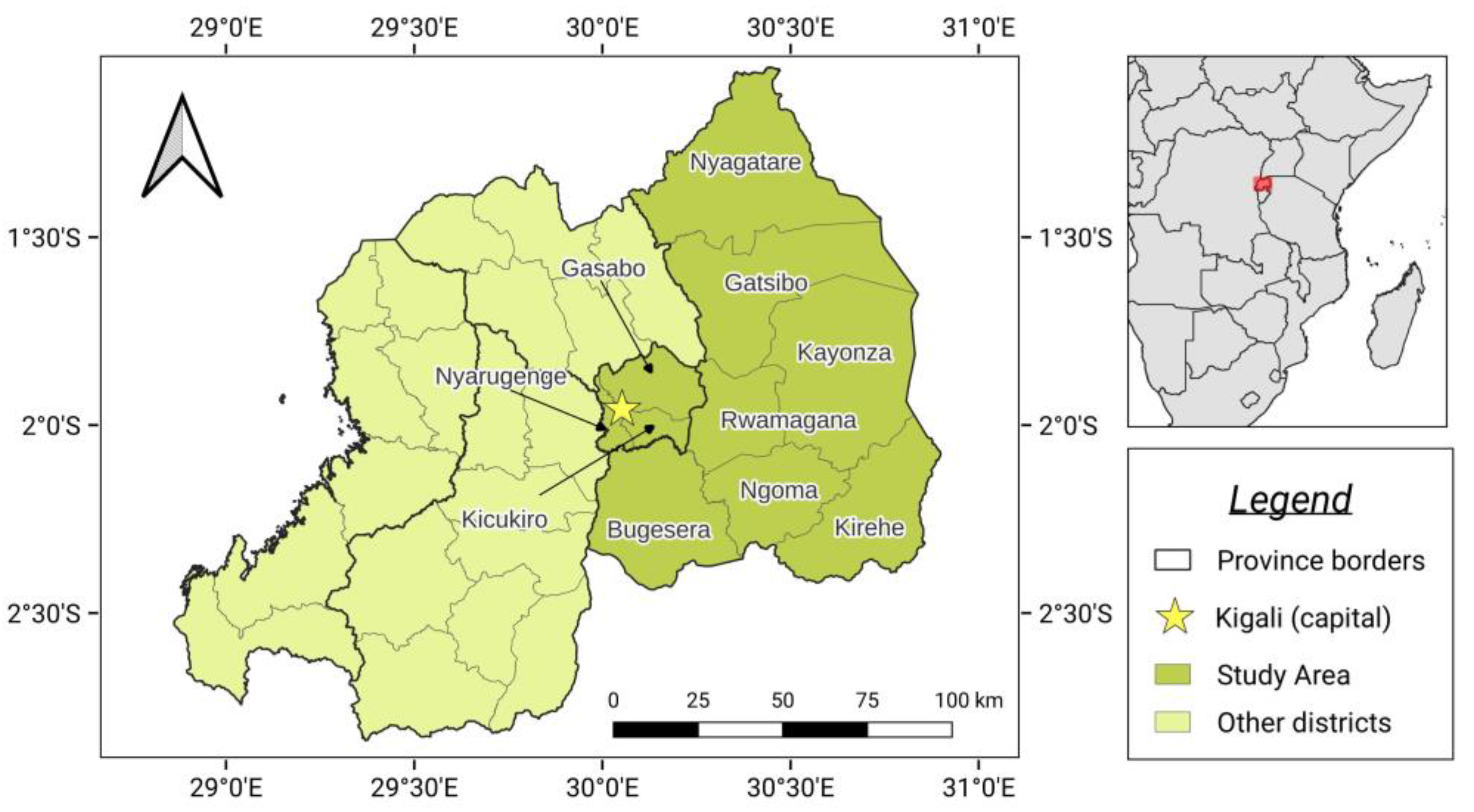
Figure 1. The study area shown within Rwanda and its location on the African continent.
Remotesensing 15 02606 g001
Figure 2. (a) Digital elevation map (m) for study area obtained from SRTM dataset [43]; (b) Mean 5-day precipitation over study area averaged from 2000–2021 from CHIRPS dataset [44].
Remotesensing 15 02606 g002
Figure 3. Additional non-spectral layers used in classification algorithm with (a) Slope as calculated from a 30 m Digital Elevation Model obtained from [43]; (b) Distance to populated areas, calculated as a raster file using data obtained from [48].
Remotesensing 15 02606 g003
Figure 4. Flowchart of methodology applied in this study.
Remotesensing 15 02606 g004
Figure 5. Land cover classes trained and predicted in this study with (a) agroforestry; (b) forest; (c) shrubland; (d) cropland; (e) grassland; (f) urban; (g) wetland; and (h) water classes.
Remotesensing 15 02606 g005
Figure 6. Instability Index (ISI) values for all Sentinel-2 spectral bands representing separability between tree classes, and between tree and non-tree classes. Separability scores shown for dry season (a) agroforestry; (c) shrubland; and (e) forest; and rainy season (b) agroforestry; (d) shrubland; and (f) forest classes.
Remotesensing 15 02606 g006
Figure 7. Accuracy scores for multiple different accuracy metrics for RF models as least-important features are recursively eliminated from the model input data. Three models are identified: M10, the model with the maximum number of input features; M10-84, the model with the highest accuracy; and M10-44, the model with the minimum number of input features.
Remotesensing 15 02606 g007
Figure 8. Average ranking of input layer categories according to their variable importance score for model M10-84. Numbers in brackets represent the number of features from each category.
Remotesensing 15 02606 g008
Figure 9. Example comparison between three models to classify forest cover in the study area with (a) location in study area; (b) Google Satellite imagery (RGB); (c) agreement between different models; (d) forest cover prediction by model M10; (e) forest cover prediction by model M10-84; (f) forest cover prediction by model M10-44.
Remotesensing 15 02606 g009
Figure 10. Example comparison between three models to classify agroforestry cover in the study area with (a) location in study area; (b) Google Satellite imagery (RGB); (c) agreement between different models; (d) agroforestry cover prediction by model M10; (e) agroforestry cover prediction by model M10-84; (f) agroforestry cover prediction by model M10-44.
Remotesensing 15 02606 g010
Figure 11. Example comparison between three models to classify shrubland cover in the study area with (a) location in study area; (b) Google Satellite imagery (RGB); (c) agreement between different models; (d) shrubland cover prediction by model M10; (e) shrubland cover prediction by model M10-84; (f) shrubland cover prediction by model M10-44.
Remotesensing 15 02606 g011
Figure 12. Land cover classification generated by the highest accuracy model M10-84, with (a) land cover classification over the entire study area; (b) detail showing the gradual eastward transition from agroforestry to shrubland cover; (c) forest cover concentrated on hilltops in the western regions; and (d) shrubland cover interspersed with grassland in the semi-arid eastern regions.
Remotesensing 15 02606 g012
Figure 13. Total area (thousands of ha) identified as agroforestry, forest, and shrubland in the National Forest Inventory [55], the Forest Cover Mapping report [54], WorldCover [73], and by models in this study.
Remotesensing 15 02606 g013
Table 1. Level-2A Sentinel-2 imagery used in this study assembled by sensing date for the dry and rainy seasons of 2018. Symbols in superscript denote Sentinel-2 tile IDs as follows: α = T36MTD, β = T35MRU, γ = T36MTC, δ = T35MRT.
Sensing Date (Dry Season)Sensing Date (Rainy Season)
01/06 α,γ,δ
08/06 α,γ,δ
11/06 α,β,γ,δ
13/06 δ
21/06 γ
23/06 α,γ
26/06 α,β,γ,δ
28/06 α,γ,δ
01/07 α,β,γ,δ
03/07 γ,δ
06/07 α,β,γ,δ
08/07 γ,δ
11/07 γ
23/07 α,γ,δ
26/07 α,β,γ,δ
31/07 α,β
02/08 α,γ,δ
07/08 α,γ,δ
15/08 γ
17/08 δ
25/08 α,β,γ,δ
27/08 α,γ,δ
01/09 γ,δ
11/09 γ
14/09 γ,δ
21/09 α,γ,δ
03/02 α,γ,δ
06/02 α,γ
21/02 α
26/02 β,δ
28/02 α,γ,δ
10/03 α,γ,δ
20/03 α,γ
25/03 α
28/03 α,γ,δ
02/04 δ
04/04 δ
14/04 δ
17/04 α,β,γ
19/04 α
27/04 α,β,γ,δ
04/05 γ
14/05 α
22/05 α,β,γ
24/05 α,γ,δ
27/05 α,β,γ,δ
29/05 α,γ,δ
Table 2. Indices and equations used in this study. The wavelengths used were as follows: B2 (Band 2; 490 nm), B8 (Band 8; 842 nm), B5 (Band 5; 705 nm), and B4 (Band 4; 665 nm). L represents a constant factor of 0.5.
IndexEquationCitation
Enhanced Vegetation Index EVI = B 8 B 4 B 8 + 6   B 4 7.5 B 2 + 1 [51]
Normalized Difference Vegetation Index (Band 8) NDVI = B 8 B 4 B 8 + B 4 [26]
Normalized Difference Vegetation Index (Band 8A) NDVI 8 A = B 8 A B 4 B 8 A + B 4 [52]
Normalized Difference Vegetation Index (Red Edge) NDRE = B 8 B 5 B 8 + B 5 [26]
Normalized Difference Water Index NDWI = B 3 B 8 B 3 + B 8 [31]
Red–Green Chlorophyll Index RGCI = B 7 B 5 1 [32]
Soil Adjusted Vegetation Index SAVI = B 8 B 4 B 8 + B 4 + L 1 + L [31]
NDVI textureStandard deviation of NDVI
(5 × 5 pixel moving window)
[27]
GLCM texture metrics
(5 × 5 pixel moving window per band)
Dissimilarity, contrast, variance, sum average, difference variance, inertia, correlation[32,49,50]
Table 3. Grid search results for three hyperparameters (numberofTrees, bagFraction, and minLeafPopulation) used to tune Random Forests algorithm. Hyperparameter values are shown in bold, model Kappa values are shown for each combination of hyperparameters, with the best model shown in bold and underlined.
numberOfTrees1005001000
bagFraction0.250.8730.8580.8520.8750.8640.8580.8740.8650.858
0.50.8680.8670.8670.8730.8700.8640.8720.8710.865
10.8660.8660.8670.8700.8700.8690.8700.8730.870
minLeafPopulation125501255012550
Table 4. Input layers for models trained in this study. F1 scores are shown for the agroforestry (AF), forest (F), and shrubland (SH) classes, with the best F1 scores for each class in bold.
Input LayersF1 Scores
Model NameSpectral Bands
(Dry)
Spectral Bands (Rainy)Vegetation
Indices
PCAPopulationSlopeDEMGLCM
Metrics
AFFSH
M1 0.5490.8140.600
M2 0.4220.6420.482
M3 0.5480.7900.572
M4 0.5860.7980.644
M5 0.6360.8640.678
M6 0.6560.8740.707
M7 0.6460.8960.698
M8 0.6450.8830.718
M9 0.6740.9040.753
M100.7110.8720.782
Table 5. Confusion matrix for model M10-84 showing predicted and actual land cover classes. Correctly identified validation pixels are shown along the diagonal (bold). User’s accuracy (UA) and producer’s accuracy (PA) values are also shown in percentages for each land cover class.
Predicted Land Cover
CropAgroforestryForestShrublandGrasslandUrbanWetlandWaterTotalPA
Actual Land CoverCropland2880791326695000403571.4
Agroforestry192314148925332200410076.6
Forest2218367612116000403391.1
Shrubland2004051393086180070401776.8
Grassland68550754135000433395.4
Urban019000401000402999.5
Wetland000000415604156100
Water000000040754075100
Total33424629430738014429403241634075
UA94.067.985.381.293.499.599.8100
Table 6. Total area (ha) in the study area classified as each tree cover type by three most accurate models used in this study. Percentages show proportion of the land cover type in the study area.
Model NameAgroforestryForestShrubland
M10397,092 (38.7%)119,917 (11.7%)167,868 (16.3%)
M10-84374,593 (36.5%)139,658 (13.6%)185,664 (18.1%)
M10-44362,740 (35.3%)139,725 (13.6%)197,211 (19.2%)
Disclaimer/Publisher’s Note: The statements, opinions and data contained in all publications are solely those of the individual author(s) and contributor(s) and not of MDPI and/or the editor(s). MDPI and/or the editor(s) disclaim responsibility for any injury to people or property resulting from any ideas, methods, instructions or products referred to in the content.