A Novel Multistage Back Projection Fast Imaging Algorithm for Terahertz Video Synthetic Aperture Radar

Abstract

Terahertz video synthetic aperture radar (THz-ViSAR) has tremendous research and application value due to its high resolution and high frame rate imaging benefits. However, it requires more efficient imaging algorithms. Thus, a novel multistage back projection fast imaging algorithm for the THz-ViSAR system is proposed in this paper to enable continuous playback of images like video. The radar echo data of the entire aperture is first divided into multiple sub-apertures, as with the fast-factorized back projection algorithm (FFBP). However, there are two improvements in sub-aperture imaging. On the one hand, the back projection algorithm (BPA) is replaced by the polar format algorithm (PFA) to improve the sub-aperture imaging efficiency. The imaging process, on the other hand, uses the global Cartesian coordinate system rather than the local polar coordinate system, and the wavenumber domain data of the full aperture are obtained step by step through simple splicing and fusion, avoiding the amount of two-dimensional (2D) interpolation operations required for local polar coordinate system transformation in FFBP. Finally, 2D interpolation for full-resolution images is carried out to image the ground object targets in the same coordinate system due to the geometric distortion caused by linear phase error (LPE) and the mismatch of coordinate systems in different imaging frames. The simulation experiments of point targets and surface targets both verify the effectiveness and superiority of the proposed algorithm. Under the same conditions, the running time of the proposed algorithm is only about 6% of FFBP, while the imaging quality is guaranteed.

1. Introduction

Synthetic aperture radar (SAR) is a high-resolution imaging radar that can operate from a long distance, in all types of weather, and throughout the day [1,2,3,4]. However, due to the low image frame rate, the conventional SAR can only obtain static target images, but not information on the moving targets, and cannot even distinguish between dynamic and static targets. Video synthetic aperture radar (Video SAR) [5] is an extension of the traditional SAR. It allows continuous video observation of the region of interest (ROI), generates a series of images during the flight of the radar platform [6], and broadcasts them in video form. Inheriting the advantages of traditional SAR, video SAR overcomes the disadvantages of traditional SAR with a low frame rate and inability to monitor in real time. Video SAR has the capability to continuously observe, and it has great potential in fields such as tracking of ground moving target indication (GMTI) and 3D imaging [7,8,9]. The frame rate usually exceeds 5 Hz to track moving targets and obtain information such as velocity and direction [10]. Furthermore, for a given resolution, the frame rate is proportional to the frequency [11], so a higher operating frequency results in a higher frame rate. With recent research on terahertz waves [12,13,14,15,16,17], terahertz video SAR (THz-ViSAR), which operates in the terahertz band, has attracted extensive attention because of its unique advantages. In contrast to traditional microwave video SAR, it can easily accomplish a high frame rate and high-resolution imaging. However, the required real-time performance will be much higher, so more efficient and applicable imaging algorithms [18] are needed.

There are a variety of imaging techniques. References [19,20,21] approximately modeled the video SAR imaging problem as tensor analysis and tensor recovery and greatly reduced the amount of required data samples during video SAR echo collection. However, in practical applications, the actual value of the tensor cannot be obtained, the rank value will also affect the error or calculation cost of the algorithms, and the dimension of vectors and matrices also imposes memory requirements. Therefore, the methods mentioned in [19,20,21] are usually suitable for specific scenarios.

For video SAR imaging in general scenes, two commonly employed approaches are the polar format algorithm (PFA) and the back projection algorithm (BPA) [22]. PFA can significantly mitigate the effects of distance migration by storing data in the polar format and has higher computational efficiency. Conventional PFA leads to the presence of residual phase errors due to the plane wave assumption, where linear phase error (LPE) leads to geometric distortion of the image [23] and quadratic phase error (QPE) results in defocusing. Its effective imaging scene radius is inversely proportional to the open square of the wavelength. Therefore, the algorithm is not applicable when dealing with large scenes and high-resolution cases.

BPA is a typical time-domain imaging algorithm introduced by computer tomography (CT) technology. It is suitable for arbitrary trajectories in any imaging mode, with accurate motion compensation capability and without assumptions and approximations. For an image with $N\times N$ pixels, its operation complexity for coherent accumulation within $N$ pulses is $N^3$. Such a large computation load greatly restricts the broad application of BPA. To this end, academics have undertaken extensive studies and proposed several methods [24,25,26,27,28,29,30,31] to reduce the computational burden of the traditional BPA and applied them to different modes [32,33,34,35,36]. The most representative ones are the fast back projection algorithm (FBP) and the fast factorized back projection algorithm (FFBP). FBP was formally proposed by A. F. Yegulalp [24] at Lincoln Laboratory, thus laying the foundation for the fast time-domain algorithm. FBP performs sub-aperture division and reconstructs the sub-images in local polar coordinates. Then, based on the geometric relationship between the sub-aperture and the scene center, the sub-images are transformed into the Cartesian coordinate system and coherently summed to obtain a full-resolution image. Although FBP is computationally efficient, it reduces image quality. FFBP, proposed by Ulander et al., has higher operational efficiency [26]. It adopts the same processing as FBP in the initial stage, but the difference is that the final image is obtained through fusion step-by-step. This process mainly realizes the mapping between coordinates using 2D interpolation operations [36], which inevitably leads to the introduction and accumulation of interpolation errors. Additionally, it is difficult for FFBP to balance efficiency and image quality and to reach its theoretical calculation amount in practical applications.

To address the contradiction between efficiency and image quality in traditional FFBP, and further improve the efficiency of the traditional imaging algorithms, this paper proposes a novel multistage back projection algorithm for THz-ViSAR fast imaging. The main technical contributions are as follows:

(1)

FFBP uses inefficient BP integration to obtain the sub-images in the initial stage. The calculation amount increases with the sub-aperture length and is close to BPA. Differently, the proposed algorithm uses more efficient PFA to process the sub-aperture data, reducing the number of interpolations in this stage.

(2)

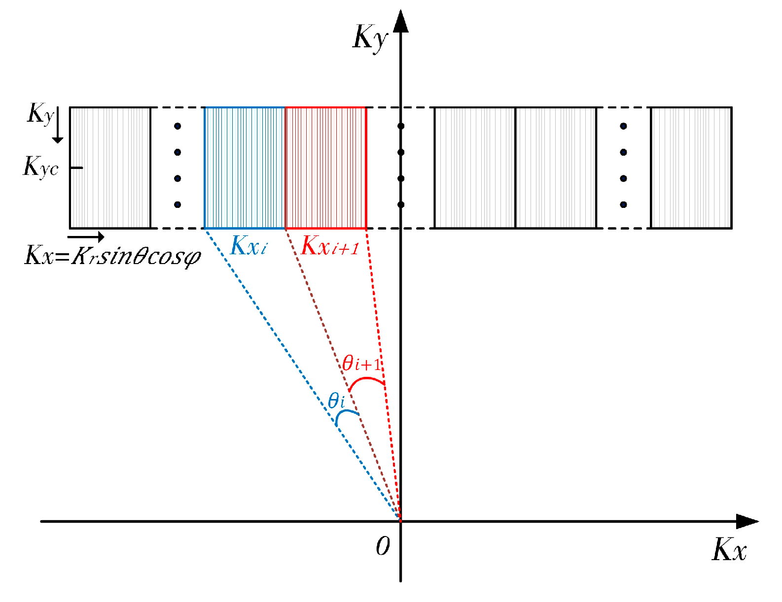
FFBP is based on local polar coordinates, and the fusion stage requires many 2D interpolations. Differently, the proposed algorithm is based on the global Cartesian coordinate with a simpler geometric configuration, and the fusion stage can be realized by wavenumber domain splicing, preventing the introduction and accumulation of interpolation errors in FFBP. Through the above improvements, the efficiency is significantly improved.

(3)

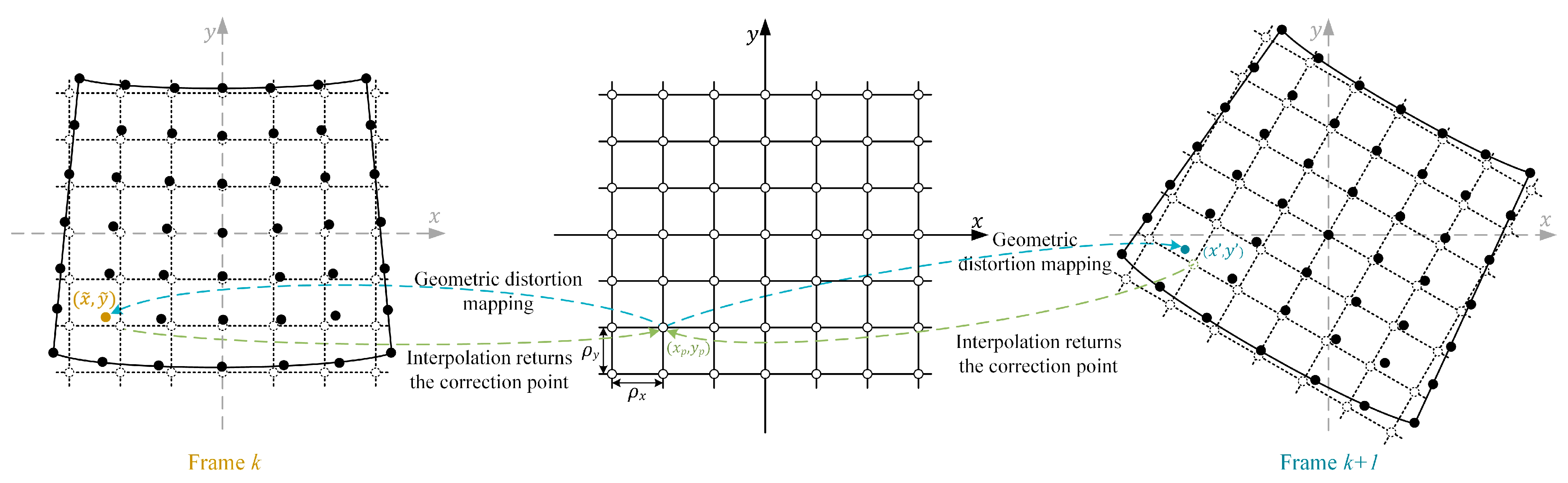
Aiming at the geometric distortion caused by linear phase error (LPE) and considering the image rotation caused by different flight trajectories, the proposed algorithm carries out 2D resampling to correct the geometric distortion and rotate the images into the same ground Cartesian coordinate.

The rest of this paper is organized as follows. Section 2 introduces the radar echo model and the FFBP algorithm. Section 3 proposes a novel imaging algorithm to address the inconsistencies existing in traditional imaging algorithms. In Section 4, the proposed algorithm is simulated and compared with the imaging result of FFBP to verify the superiority of the proposed algorithm. Finally, the conclusions are drawn in Section 5.

2. Materials

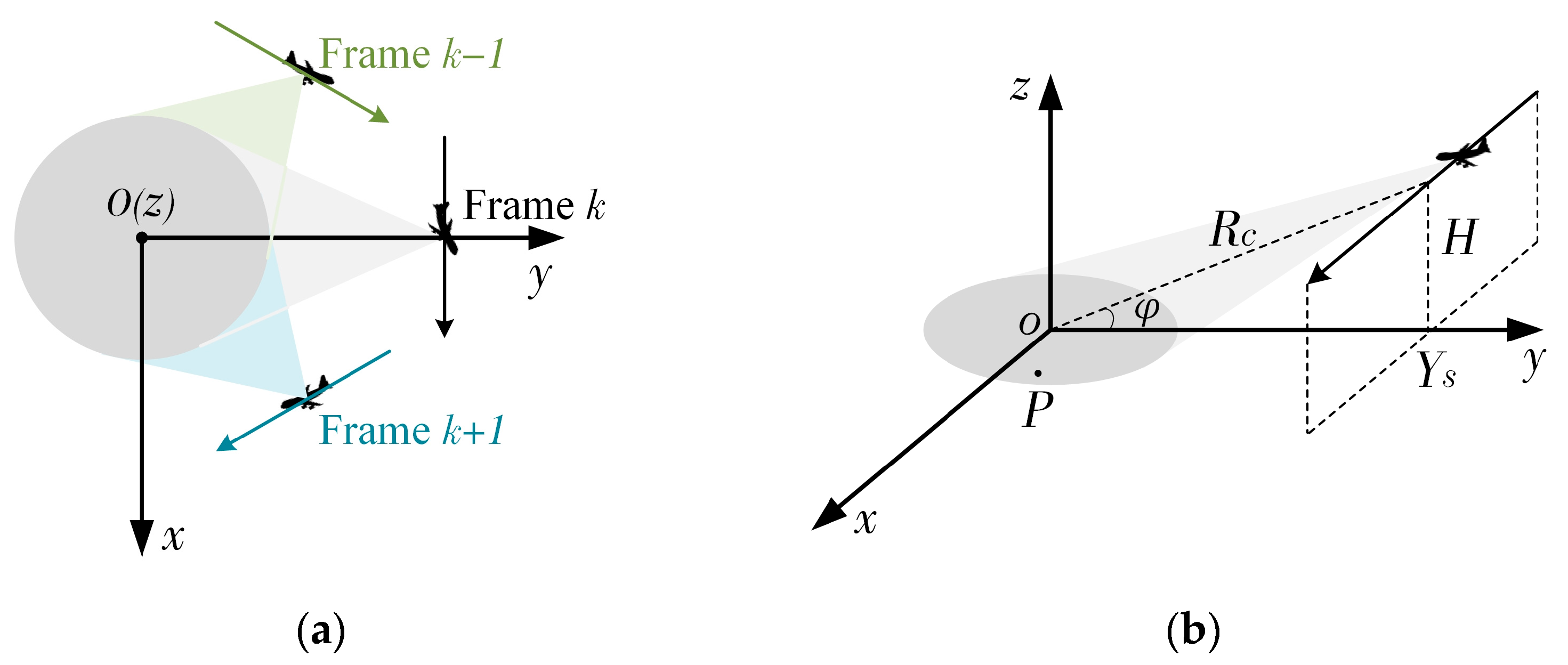
2.1. Radar Echo Model

In a typical THz-ViSAR imaging mode, the radar platform is in linear spotlight mode during the flight of each frame. In this mode, SAR can continuously monitor the region of interest (ROI) while obtaining images to generate video. The imaging geometry configuration is shown in Figure 1. The top view is shown in (a), where green, black, and blue lines correspond to the flight trajectory of the $k-1$, $k$, and $k+1$ frames, respectively, and each frame is in linear spotlight mode. Taking frame $k$ as an example, its 3D view is shown in Figure 1b. During the data collection, the platform flies at a constant elevation angle $\phi$. The shaded area is the irradiation scene, and the coordinate origin O is the scene’s center. The radar platform makes a uniform linear motion with velocity $V_a$, and its instantaneous position is $(V_a{t}_a,Y_s,H)$. The radar assumes transmit linear frequency modulation (LFM) signal, as shown in (1).

$$s_t(t_a,t_r)=rect\left(\frac{t_r}{T_r}\right)exp\left\{j2\pi \left(f_c{t}_r+\frac{1}{2}\gamma t_r^2\right)\right\},$$

(1)

where $t_a$ is the azimuth slow time, $t_r$ is the range fast time, $T_r$ is the pulse width, $f_c$ is the center frequency, modulation frequency $\gamma =B/T_r$, $B$ is the bandwidth, and $rect\left(·\right)$ is rectangular window function.

For any point target P ($x$, $y$, 0) in the scene, the instantaneous slant range from the radar platform to point P is:

$$R_p=\sqrt{{(V_a{t}_a-x)}^2+{(Y_s-y)}^2+H^2},$$

(2)

Therefore, the echo signal of the target is expressed as:

$$s_r(t_a,t_r)=rect\left(\frac{t_r-\tau }{T_r}\right)exp\left\{j2\pi \left(f_c\left(t_r-\tau \right)+\frac{1}{2}\gamma {\left(t_r-\tau \right)}^2\right)\right\},$$

(3)

where time delay $\tau =2R_p/c$.

Since the radar operates in the THz band, dechirping is frequently used to receive the echo, lowering the frequency bandwidth of the signal and, thus, reducing the stress on the hardware. Combining the imaging geometry shown in Figure 1, the slant range from the scene center O to the radar platform is selected as the reference range, i.e.,

$$R_{ref}=\sqrt{{\left(V_a{t}_a\right)}^2+Y_s^2+H^2},$$

(4)

Then, the reference signal is shown as:

$$s_{ref}\left(t_a,t_r\right)=rect\left(\frac{t_r-{\tau }_{ref}}{T_{ref}}\right)exp\left\{j2\pi \left(f_c\left(t_r-{\tau }_{ref}\right)+\frac{1}{2}\gamma {\left(t_r-{\tau }_{ref}\right)}^2\right)\right\},$$

(5)

where time delay ${\tau }_{ref}=2R_{ref}/c$, and $T_{ref}$ is the pulse width of the reference signal, which is larger than $T_r$. The differential frequency signal, as shown in (6), is obtained by mixing the reference signal (5) with the echo (3), and the differential range $\Delta R=R_p-R_{ref}$.

$$s_{if}\left(t_a,t_r\right)=s_r\left(t_a,t_r\right)·s_{ref}^{\mathrm{*}}\left(t_a,t_r\right)=rect\left(\frac{t_r-\tau }{T_r}\right)\mathit{exp}\left(-j\frac{4\pi f_c}{c}\Delta R\right)·exp\left[-j\frac{4\pi }{c}\gamma \left(t_r-{\tau }_{ref}\right)\Delta R\right]exp\left(-j\frac{4\pi }{c^2}\gamma {\Delta R}^2\right),$$

(6)

2.2. Review of FFBP

FFBP is a classical time-domain imaging algorithm that significantly improves the operational efficiency of the traditional back projection algorithm. Reference [26] notes that FFBP requires the least interpolations when the factorization factor is the natural logarithm $e$. Practically, only integers can be taken, so 2 or 4 are often taken as the base. The flow chart of the algorithm with base two is shown in Figure 2.

Firstly, FFBP divides the whole synthetic aperture into several shorter sub-apertures and performs back projection in local polar coordinates to obtain sub-images. Each sub-image has a full resolution in range and a lower resolution in azimuth. Then, two adjacent sub-images are coherently fused to obtain an image with higher azimuthal resolution in a new polar coordinate system. As the recursive fusion proceeds, the azimuthal resolution of sub-images increases. Finally, the polar coordinate image is transformed into the Cartesian coordinate system, and the full-resolution image is obtained.

However, there are still many drawbacks to this algorithm. The algorithm still uses inefficient BPA to reconstruct sub-images. Moreover, the mapping between different coordinate systems during image fusion requires several 2D interpolations, which will inevitably introduce interpolation errors. As the fusion proceeds gradually, the errors will be accumulated and amplified continuously, eventually lowering the image quality. The image quality can be improved by lengthening the sub-aperture or using a more accurate interpolation kernel, which will sacrifice the algorithm’s efficiency [37,38]. Therefore, it is difficult for FFBP to reach the theoretical computing capacity in practical applications, and it is usually challenging to achieve high image quality with less computational burden. Notably, the algorithm does not consider the rotation of the images due to different flight trajectories. Therefore, it is urgent to improve the imaging algorithm for the THz-ViSAR system.

3. Methods

The efficiency of the imaging algorithm is crucial to the ViSAR system, which is related to whether ViSAR can realize real-time observation of ROI. Unfortunately, the traditional FFBP requires numerous 2D interpolations to achieve image fusion, significantly affecting the algorithm’s efficiency and even the image quality. This paper proposes a novel multistage back projection algorithm to address these problems.

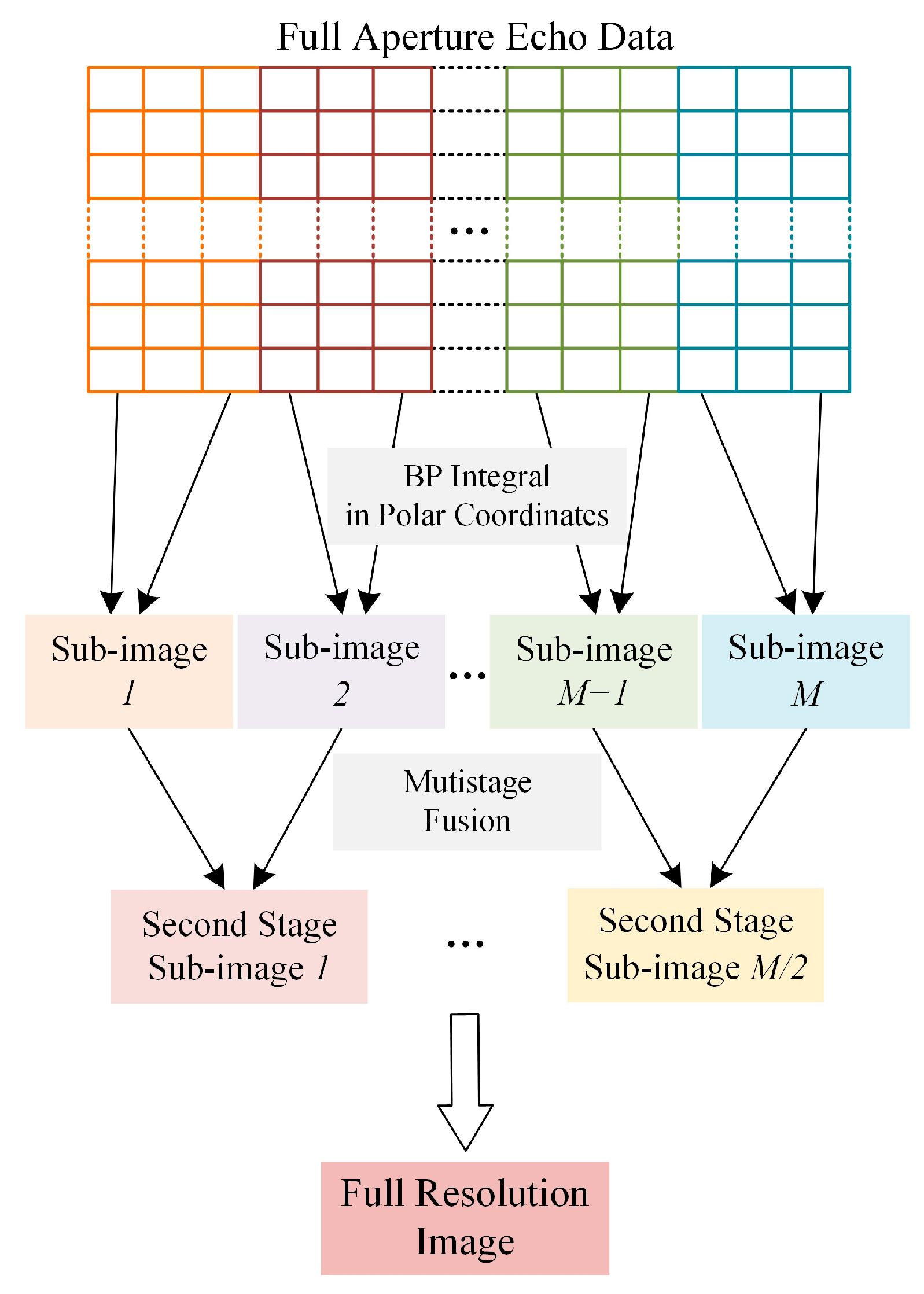
3.1. Principle of the Proposed Algorithm

For the above imaging geometry, the principle and processing flow of the proposed algorithm is described as follows. In the initial stage, the full aperture (length of $L_a$) is divided. If the number of sub-apertures is $M$, the sub-aperture length is $l=L_a/M$, and the global Cartesian coordinate system with the center of the full aperture as the origin is established. Figure 3 depicts the sub-apertures’ division and the coordinate system’s establishment. The direction of flight is taken as the positive x-axis, the direction perpendicular to the flight path and pointing to the center of the scene is taken as the positive y-axis, and the center of the full aperture is taken as the origin. Figure 3 is illustrated in a two-dimensional coordinate system to simplify the geometric configuration.

In this case, the differential frequency signal is expressed as:

$$s_{if}\left(t_a^{\left(i\right)},t_r\right)=rect\left(\frac{t_r-\tau }{T_r}\right)\mathit{exp}\left(-j\frac{4\pi f_c}{c}\Delta R\right)·exp\left[-j\frac{4\pi }{c}\gamma \left(t_r-{\tau }_{ref}\right)\Delta R\right]exp\left(-j\frac{4\pi }{c^2}\gamma {\Delta R}^2\right),$$

(7)

where time delay $\tau =2R_p/c$, the instantaneous slant range $R_p\left(t_a^{\left(i\right)}\right)$ from target P to the sub-aperture $i(i=\mathrm{1,2}\dots M)$, and the azimuth slow time $t_a^{\left(i\right)}$ of the sub-aperture $i$ are shown in (8) and (9), respectively.

$$R_p\left(t_a^{\left(i\right)}\right)=\sqrt{{\left(V_a{t}_a^{\left(i\right)}-x\right)}^2+{\left(Y_s-y\right)}^2+H^2,}$$

(8)

$$t_a^{\left(i\right)}\in \left[-\frac{L_{\mathrm{a}}}{2V_a}+\frac{\left(i-1\right)l}{V_a},-\frac{L_{\mathrm{a}}}{2V_a}+\frac{il}{V_a}\right),$$

(9)

The differential frequency signal (7) is converted to the range frequency domain by range fast Fourier transform (FFT), as shown in (10).

$$s_{if}\left(t_a^{\left(i\right)},f_r\right)=T_{r}sinc[T_r(f_r+\frac{2\gamma }{c}∆R)]\mathit{exp}\left(-j\frac{4\pi f_c}{c}\Delta R\right)exp(-j\frac{4\pi f_r}{c}\Delta R)exp\left(-j\frac{4\pi \gamma }{c^2}{\Delta R}^2\right),$$

(10)

where $f_r$ is the range frequency.

The last two terms are the oblique item and the remaining video phase (RVP), respectively, which need to be removed by multiplying with the compensation function (11).

$$H_{RVP}=\mathit{exp}\left(-j\frac{\pi f_r^2}{\gamma }\right),$$

(11)

Then, range fast inverse Fourier transform (IFFT) is performed and the result is shown in (12).

$$s_i\left(t_a^{\left(i\right)},t_r\right)=rect\left(\frac{t_r-\tau }{T_r}\right)exp\left[-j{K}_r\Delta R\right],$$

(12)

where the wave number $K_r=\frac{4\pi }{c}(f_c+f_r)$.

If the plane wave-front hypothesis is adopted, the differential distance $\Delta R=R_p-R_{ref}$ can be expanded by the Taylor series as:

$$\Delta R=-x\frac{V_a{t}_a^{\left(i\right)}}{\sqrt{{\left(V_a{t}_a^{\left(i\right)}\right)}^2+Y_s^2+H^2}}-y\frac{Y_s}{\sqrt{{\left(V_a{t}_a^{\left(i\right)}\right)}^2+Y_s^2+H^2}}+\xi \left(x,y\right)+o\left(x,y\right),$$

(13)

where $\xi \left(x,y\right)$ is a second-order Taylor series expansion, and $o\left(x,y\right)$ is a third-order and higher-order term. This equation can be simplified to (14).

$$\Delta R\approx -xsin\theta cos\phi -ycos\theta cos\phi ,$$

(14)

where $\phi$ is the elevation angle, $\theta$ is the azimuth accumulation angle, and

$$\left\{\begin{array}{c}cos\phi =\frac{\sqrt{{\left(V_a{t}_a^{\left(i\right)}\right)}^2+Y_s^2}}{\sqrt{{\left(V_a{t}_a^{\left(i\right)}\right)}^2+Y_s^2+H^2}}\\ sin\theta =\frac{V_a{t}_a^{\left(i\right)}}{\sqrt{{\left(V_a{t}_a^{\left(i\right)}\right)}^2+Y_s^2}}\\ cos\theta =\frac{Y_s}{\sqrt{{\left(V_a{t}_a^{\left(i\right)}\right)}^2+Y_s^2}}\end{array},\right.$$

(15)

Then, (12) can be written as:

$$s_i(K_x,K_y)=rect\left(\frac{t_r-\tau }{T_r}\right)exp\left[j(x{K}_x+y{K}_y)\right],$$

(16)

where the azimuth and range wavenumber are, respectively:

$$\left\{\begin{array}{c}{K}_x=K_{r}sin\theta cos\phi \\ K_y=K_{r}cos\theta cos\phi \end{array},\right.$$

(17)

At this point, the data in polar format are converted to the Cartesian format by range interpolation and azimuth interpolation, respectively. Then, since there is no need to output sub-images, the multistage fusion is performed in the wavenumber domain (shown in Figure 4).

If the total number of stages is $G$, for stage $g(g=\mathrm{1,2}\dots G)$, the number of sub-apertures is represented by $K_g$. For example, the number of sub-apertures in the initial stage, $K_1=2^{G-1}$. $s_i^g\left(K_x,K_y\right)$, is used to represent the wavenumber domain data of stage $g$ and sub-aperture ${i(i=\mathrm{1,2}\dots K}_g)$. Since the proposed algorithm adopts the global Cartesian coordinate system with the center of the full aperture as the origin, wavenumber domain splicing is adopted in this paper to achieve the fusion stage, and the process can be expressed as (18).

$$s_i^g\left(K_x,K_y\right)=\left[\left(s_{2i-1}^{g-1}\left(K_x,K_y\right)\right);\left(s_{2i}^{g-1}\left(K_x,K_y\right)\right)\right],$$

(18)

The wavenumber domain data of two adjacent sub-apertures are spliced to obtain the wavenumber domain data of the larger sub-apertures, and the azimuth resolution is increased two times. The procedure is repeated until the full-aperture wavenumber domain data (i.e., $s(K_x,K_y)$) are obtained. Then, 2D IFFT is performed for $s(K_x,K_y)$ to obtain the full-resolution image, described as:

$$I\left(x,y\right)=\iint s(K_x,K_y)exp[-j\left(x{K}_x+y{K}_y\right)]dxdy,$$

(19)

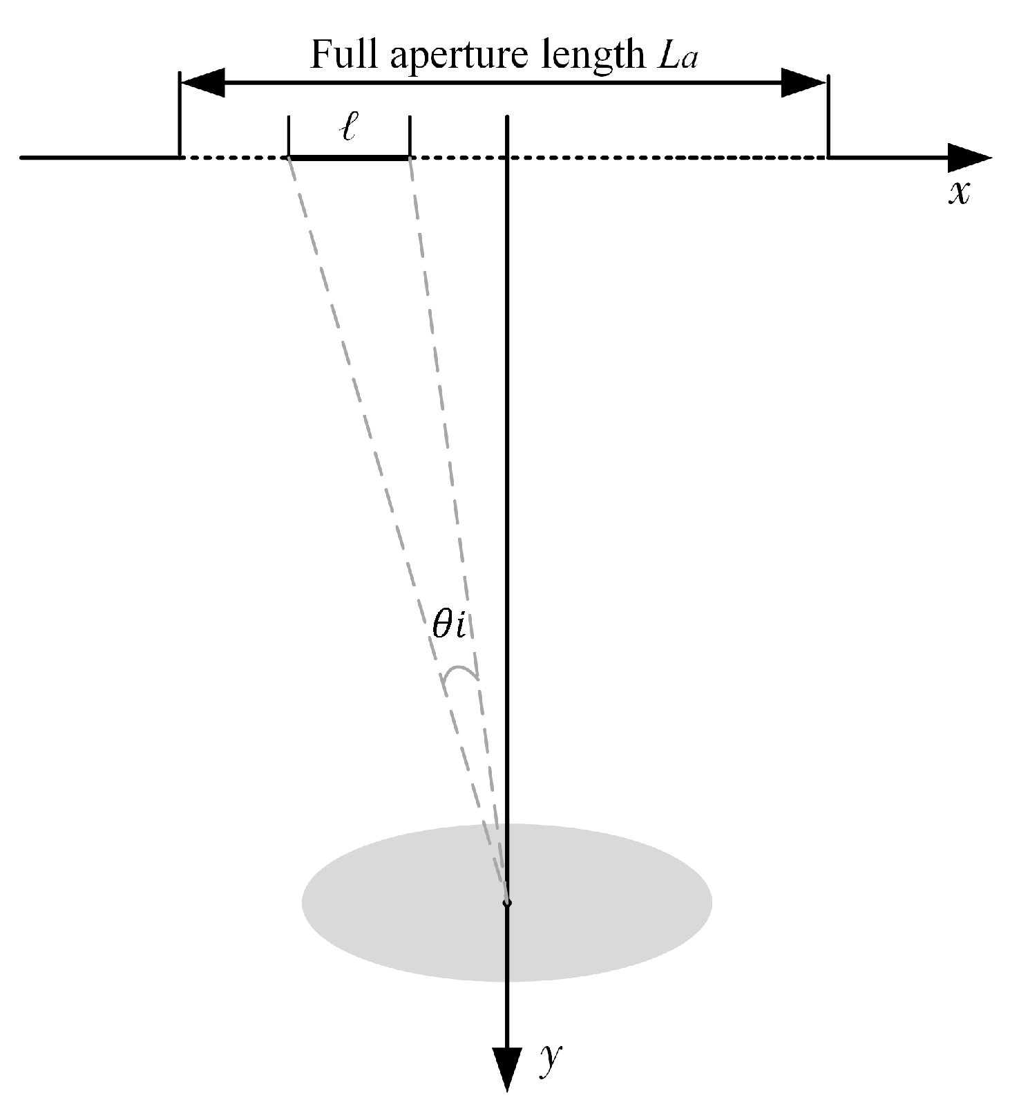
3.2. Geometric Distortion Analysis and Correction

Since the proposed algorithm extends $\Delta R$ to (14) based on the far-field assumption, leading to linear, quadratic, and higher-order phase errors, the linear phase error will cause image distortion, and the quadratic phase error will defocus the image. As shown in (12), its phase can be expressed as:

$$\mathsf{\Phi }=K_r\Delta R=K_r\left(R_p-R_{ref}\right),$$

(20)

The phase $\mathsf{\Phi }$ can be rewritten as a Taylor expansion at the center $(K_x=0,K_y=K_{yc})$ of 2D wavenumber domain [39]:

$$\mathsf{\Phi }=a_0+a_x{K}_x+a_y\left(K_y-K_{yc}\right)+a_{xx}{K}_x^2+a_{yy}{\left(K_y-K_{yc}\right)}^2+a_{xy}{K}_x\left(K_y-K_{yc}\right)+\dots ,$$

(21)

After formula derivations, the first-order and second-order coefficients $a_x$, $a_y$, $a_{xx}$, and $a_{yy}$ can be calculated as:

$$a_x={\left.\frac{\partial \mathsf{\Phi }}{\partial K_x}\right|}_{K_x=0,K_y=K_{yc}}=\frac{-x{Y}_s}{\alpha cos\phi },$$

(22)

$$a_y={\left.\frac{\partial \mathsf{\Phi }}{\partial K_y}\right|}_{K_x=0,K_y=K_{yc}}=\frac{\alpha -R_c}{cos\phi },$$

(23)

$$a_{xx}={\left.\frac{{\partial }^2\mathsf{\Phi }}{\partial K_x^2}\right|}_{K_x=0,K_y=K_{yc}}=\frac{\alpha -R_c}{K_{yc}cos\phi }+\frac{Y_s^2}{K_{yc}cos\phi }\left(\frac{-x^2}{{\alpha }^3}+\frac{1}{\alpha }-\frac{1}{R_c}\right),$$

(24)

$$a_{yy}={\left.\frac{{\partial }^2\mathsf{\Phi }}{\partial K_y^2}\right|}_{K_x=0,K_y=K_{yc}}=0,$$

(25)

where $\alpha =\sqrt{x^2+{(Y_s-y)}^2+H^2}$, and $R_c=\sqrt{Y_s^2+H^2}$.

The first-order terms $a_x$, $a_y$ cause geometric distortion. Additionally, the offset coordinate of the target $(x,y)$ in the image is

$$\left\{\begin{array}{c}\tilde{x}=\frac{x{Y}_s}{\alpha cos\phi }\\ \tilde{y}=\frac{\alpha -R_c}{cos\phi }\end{array}\right.,$$

(26)

where $\tilde{x}$ and $\tilde{y}$ are the distorted azimuth and range coordinates, respectively. Therefore, the target position offset in each sub-image in the initial stage is consistent, and then as the fusion stage continues, the geometric distortion in each image in each step is also consistent. In other words, the target position offset in the full-resolution image also conforms to (26).

To describe the image distortion more directly, $r_e$ is defined as the range error between the true position $(x,y)$ and the offset position $(\tilde{x},\tilde{y})$ of the point targets.

$$r_e=\sqrt{{\left(x-\tilde{x}\right)}^2+{\left(y-\tilde{y}\right)}^2},$$

(27)

Figure 5 shows the range error in the whole scene, in which the solid red line is the contour with a range error of 1 m, and the solid green line is the contour with a distance error of 0.1 m. It is easy to find that the closer the point target is to the center, the smaller the range error is, and vice versa. For example, the range error of the point at (50, 50) is larger than 1 m, which is almost equivalent to ten resolution units (resolution of 0.12 m). The ViSAR system usually requires the target to be positioned at the actual location in the image, so geometric distortion correction [40] of the image is essential.

It should be noted that when there is an angle $\vartheta$ between the flight trajectories of different frames (see Figure 1a), the proposed algorithm reconstructs the image in a Cartesian coordinate centered on the full aperture, which results in a corresponding angular rotation of the full-resolution image. The rotation is shown in (28).

$$\left.\left[\begin{array}{c}{x}^{\prime }\\ y^{\prime }\end{array}\right.\right]=\left[\begin{array}{cc}cos\vartheta & -sin\vartheta \\ sin\vartheta & cos\vartheta \end{array}\right]\left.\left[\begin{array}{c}\tilde{x}\\ \tilde{y}\end{array}\right.\right],$$

(28)

However, each frame should be built in the coordinate system with the scene center as the origin. Therefore, each point $(x^{\prime },y^{\prime })$ in the image needs to be corrected and rotated into the ground coordinate system, and its principle is shown in Figure 6.

As can be seen from (26) and (28), the corresponding offset position $(\tilde{x},\tilde{y})$ or $(x^{\prime },y^{\prime })$ in the full-resolution image can be obtained according to the real position coordinates $(x,y)$ of the ground point target. Furthermore, the mapping relationship between them is known so that the correction can be realized by image domain resampling. Firstly, the correction area is selected, and the correction grid is divided, as shown in Figure 6. The correction points are evenly distributed in the $xy$ coordinate system, and the horizontal and vertical intervals of adjacent correction points are ${\rho }_x$, ${\rho }_y$, respectively. For each correction point $(x_p,y_p)$, its coordinates $(\tilde{x},\tilde{y})$ or $(x^{\prime },y^{\prime })$ in the full-resolution image are calculated, and then the correction point is returned from this coordinate in the full-resolution image by bilinear interpolation so that the correction of a single correction pixel is achieved. Then, the above process is repeated for all pixels of the full-resolution image. While realizing geometric distortion correction, the images are rotated into the same ground coordinate system.

The quadratic terms $a_{xx}$, $a_{yy}$ are space-variable functions [41], which will defocus the image. Moreover, the farther the target is from the scene’s center, the more severe the defocusing is. Therefore, the QPE leads to the scene size limitation, and the quantitative expressions for the maximum allowable scene radius are given in (29).

$$r_{\pi /4}={\rho }_a\sqrt{\frac{R_c}{{\lambda }_c}},$$

(29)

where $r_{\pi /4}$ is the scene radius using $\pi /4$ as the allowable quadratic phase error. From (29), it is known that the allowed scene radius is inversely proportional to the square root of the wavelength ${\lambda }_c$, or proportional to the square root of the center frequency. Once the imaging region does not satisfy this limitation, the image requires phase error correction. Generally, it is challenging to correct QPE with spatial post-processing [42,43]. Fortunately, this paper considers the characteristics of the small imaging region of THz-ViSAR and the large allowable radius of QPE. This paper considers that QPE can be ignored, i.e., all targets in the whole scene have good focusing performance.

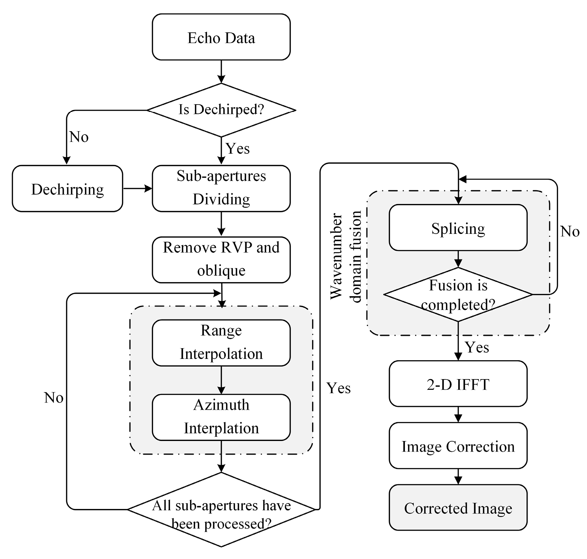
3.3. Algorithm Processing Flow

The proposed algorithm flow chart is shown in Figure 7, and the key steps are as follows. Firstly, the aperture division is performed, and the below processes are carried out separately in the global Cartesian coordinate: removal of RVP and oblique items, range and azimuth interpolation. Then, two adjacent sub-apertures are spliced in the wavenumber domain, which is repeated until the full aperture wavenumber domain is obtained. Furthermore, the full-resolution image is obtained using 2D IFFT. Finally, correction is performed to obtain the final image.

Compared with traditional FFBP, the proposed algorithm has the following advantages. Firstly, the reconstruction of sub-images abandons the inefficient BPA and only requires fewer interpolation operations [44,45,46,47]. Secondly, the global Cartesian coordinate is used to replace local polar coordinates. Compared with the latter, the former has a simpler geometric structure and is easier to implement programmatically. Moreover, simple wavenumber domain splicing can realize the fusion stage, thus avoiding introduction and accumulation of interpolation errors. Therefore, the proposed algorithm further reduces the processing complexity of the traditional imaging algorithm. Last, the geometric distortion and rotation between different frames are considered and corrected in this paper.

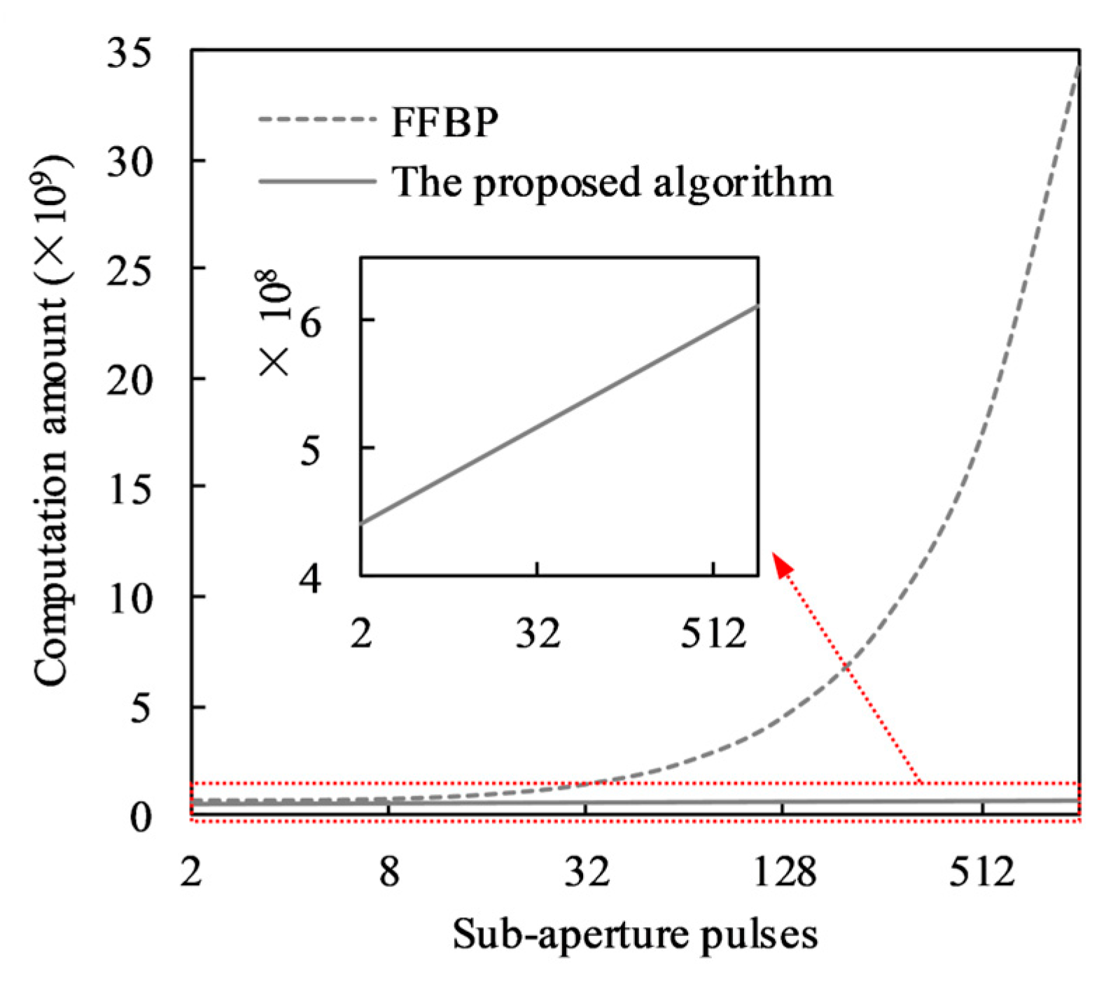
3.4. Computing Load Analysis

Assume that the number of pulses contained in the full aperture is $N$, and the full-resolution image contains $N\times N$ pixels. The full aperture is divided into $N/n$ sub-apertures containing $n$ pulses. According to the algorithm processing flow, the calculation amount is analyzed as follows:

The following processing for each sub-aperture data is performed separately.

(1) Removal of RVP and oblique items requires the following operations: range FFT ($Nn{\log }_2\sqrt{N}$), multiplied by the compensation function ($Nn$) and range IFFT ($Nn{\log }_2\sqrt{N}$).

(2) Range interpolation is realized via range FFT ($Nn{\log }_2\sqrt{N}$), 8-fold up-sampling, and range IFFT (8$Nn{\log }_2\sqrt{8N}$).

(3) Azimuth interpolation is realized via azimuth FFT ($Nn{\log }_2\sqrt{n}$), 8-fold up-sampling, and azimuth IFFT (8$Nn{\log }_2\sqrt{8n}$).

Thus, the number of complex multiplication operations required for each sub-aperture processing at the initial stage is $25Nn+11Nn{\log }_2\sqrt{N}+9Nn{\log }_2\sqrt{n}$. Therefore, the number of complex multiplication operations dealing with $N/n$ sub-apertures data is $N/n(25Nn+11Nn{\log }_2\sqrt{N}+9Nn{\log }_2\sqrt{n})$, i.e., $25N^2+11N^2{\log }_2\sqrt{N}+{9N}^2{\log }_2\sqrt{n}$.

Then, the wavenumber domain fusion stage is realized via splicing, and the number of multiplications in this stage can be ignored. Additionally, the multiplication times of 2D IFFT to get the full-resolution image is ${2N}^2{\mathit{log}}_2\sqrt{N}$. Finally, the image correction is achieved via bilinear interpolation ($4N^2$).

Summing up the above, the total multiplications of the algorithm in this paper are $29N^2+13N^2{\log }_2\sqrt{N}+{9N}^2{\log }_2\sqrt{n}$. Additionally, through calculation, the total multiplications required by FFBP under the same conditions are $8n{N}^2+16N^2{\mathit{log}}_{2}N/n$.

Set $N=2048$ to compare the computation burden of the proposed algorithm and FFBP, as shown in Figure 8. It is not difficult to find that the computation amount of FFBP increases with the increase of the number of sub-aperture pulses $n$, and the trend is significant. However, the changing trend of the proposed algorithm is much slower and lower than FFBP. Therefore, the proposed algorithm has higher efficiency. The area in the red box is enlarged as shown in the figure. It can be seen that the computing load of the proposed algorithm increases monotonically with the number of sub-aperture pulses $n$. In other words, the larger the $n$, the longer the sub-aperture length, and the larger the arithmetic amount. However, $n$ cannot be infinitesimally small, resulting in a low azimuth resolution of the sub-images. Therefore, the value of $n$ should be selected according to the practical application.

4. Results

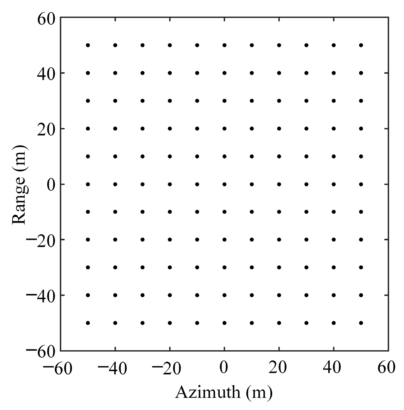
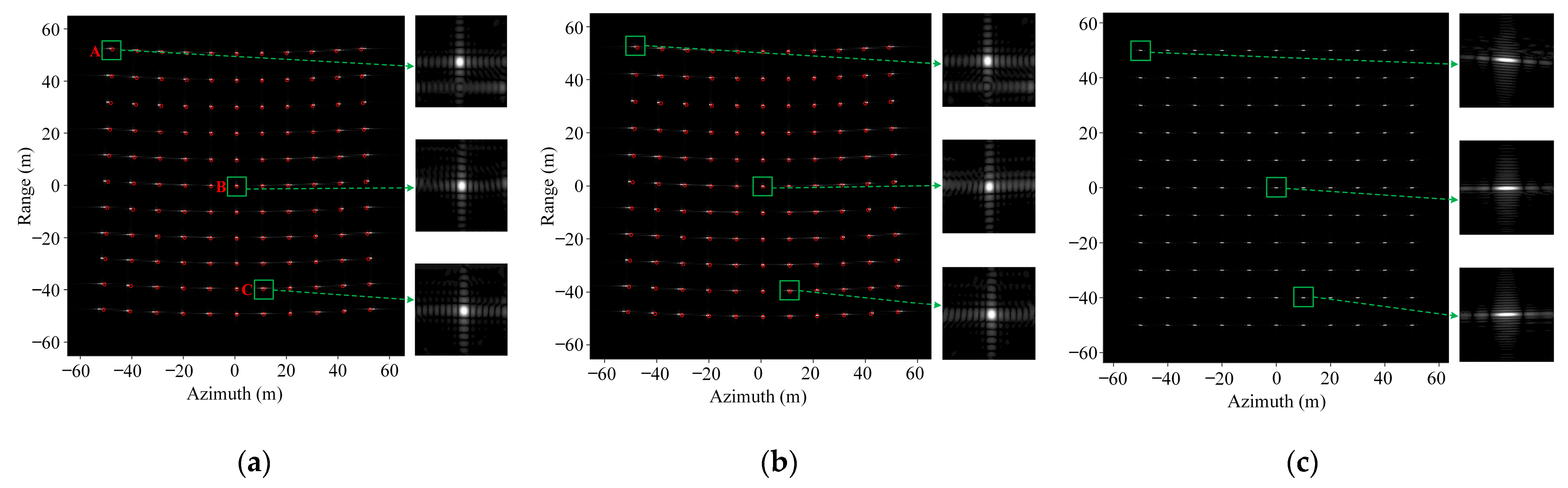
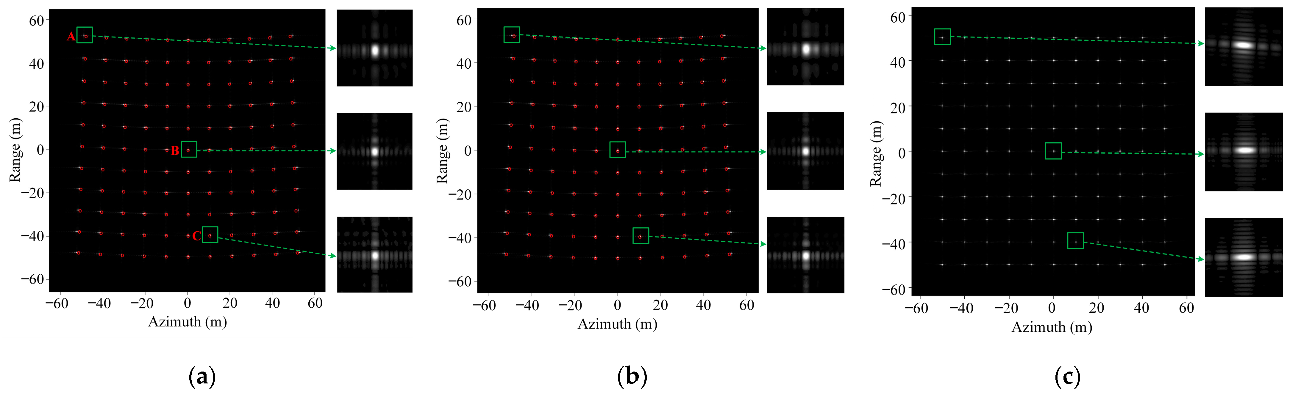
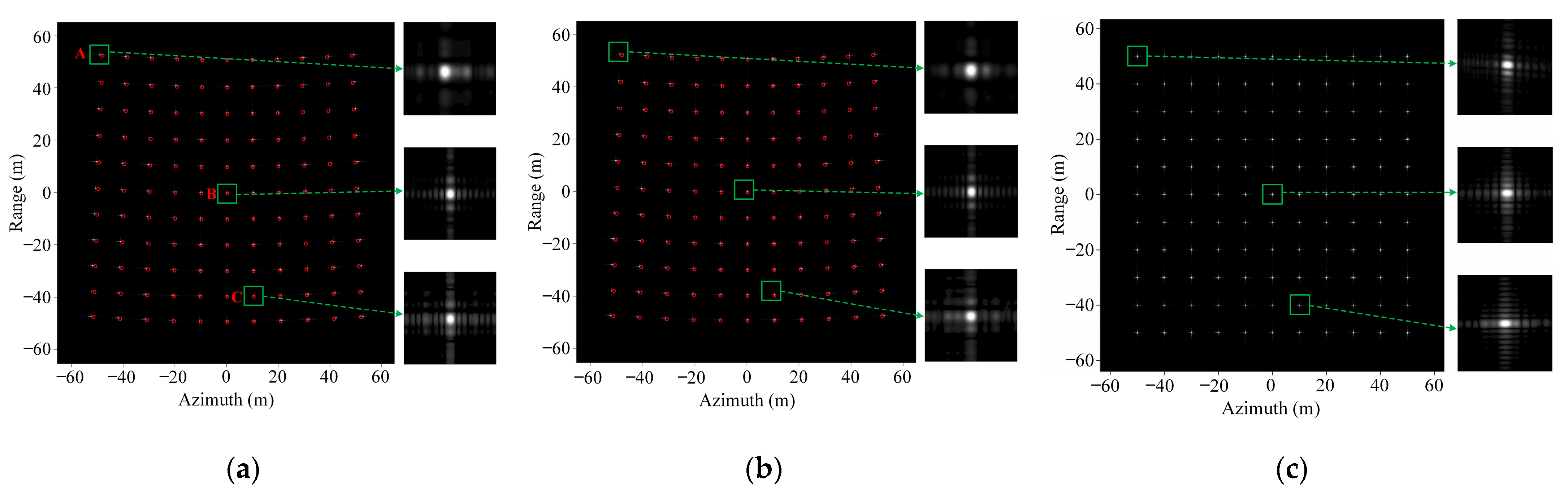
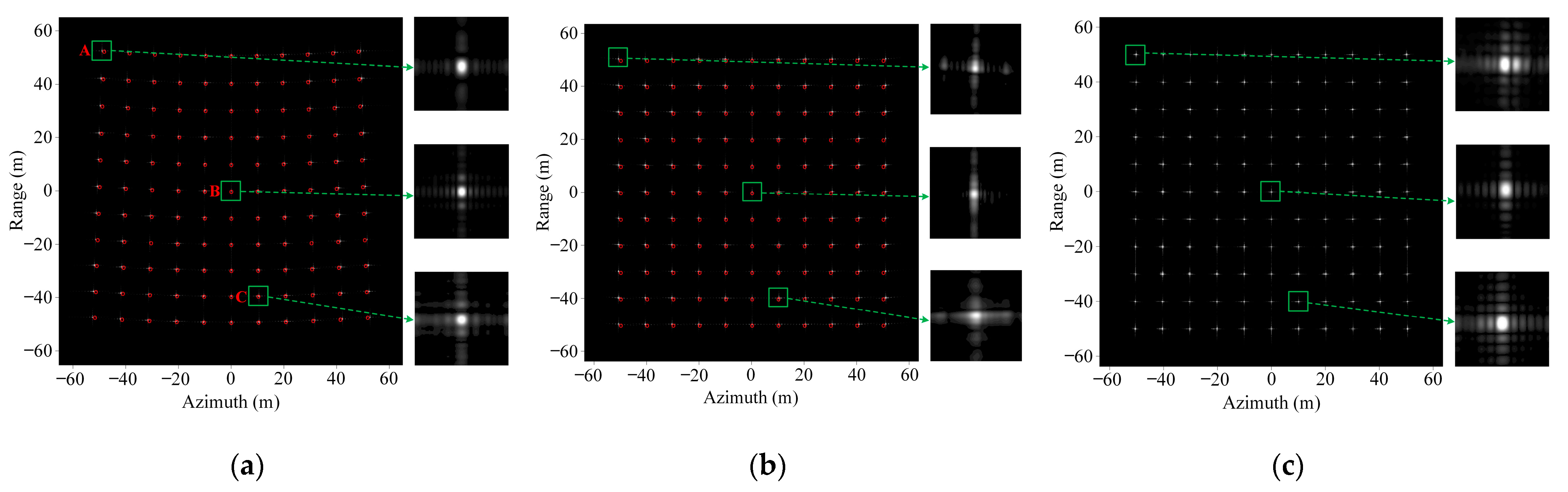
4.1. Point Targets Simulation Results

The simulation experiments were conducted in this paper to verify the proposed algorithm’s effectiveness and superiority. The main radar system parameters for the simulation experiment are shown in

Table 1. Radar system parameters.

Parameters	Explain	Value
$f_c$	center frequency	220 GHz
$B$	bandwidth	1.2 GHz
$T_r$	pulse width	50 μs
$\phi$	elevation angle	45°
$R_c$	slant range of scene center	1 km
$V_a$	flight speed	50 m/s
$r_i$	radius of the imaging area	60 m
${\rho }_r$	range resolution	0.12 m
${\rho }_a$	azimuth resolution	0.12 m

, which were used to simulate the echo data. There are 11 × 11 point targets evenly distributed in the scene (see Figure 9). The final imaging grid’s pixel points are 2048 × 2048 (Range × Azimuth). The theoretical value of 2D resolution is about 0.12 m × 0.12 m (Range × Azimuth). Here, the whole synthetic aperture is divided into eight sub-apertures, and each sub-aperture contains 256 pulses. Both algorithms adopt two as the radix for fusion in this simulation experiment.

Some images of each stage and their geometric distortion are given. For example, eight sub-apertures are divided in this paper; both algorithms have four steps. Firstly, eight sub-images can be obtained in the initial stage, and some of them were selected for illustration, as shown in Figure 10. In these images, the red dots indicate the theoretical point target locations and the white dots indicate the distribution during imaging. It can be seen that the target position offset in each sub-image in the initial stage is the same and follows the theoretical situation.

Three targets, A, B, and C, were enlarged, and their focusing effects were analyzed. The results of impulse response width (IRW), peak sidelobe ratio (PSLR), and integral sidelobe ratio (ISLR) are shown in

Table 2. IRW, PSLR, and ISLR values of point targets A/B/C in the initial step sub-images.

		Sub-Image 1 of the Proposed Algorithm (A/B/C)	Sub-Image 2 of the Proposed Algorithm (A/B/C)	Sub-Image 1 of FFBP (A/B/C)
IRW (m)	Range	0.16/0.15/0.16	0.16/0.16/0.15	0.16/0.15/0.15
	Azimuth	1.03/0.99/1.04	1.01/0.97/1.02	0.93/0.97/0.98
PSLR (dB)	Range	−12.90/−13.31/−13.16	−12.95/−13.22/−13.04	−13.30/−13.43/−13.26
	Azimuth	−12.38/−12.97/−12.88	−12.33/−11.69/−12.53	−17.80/−11.79/−12.70
ISLR (dB)	Azimuth	−28.49/−29.21/−31.64	−28.43/−30.35/−28.63	−26.70/−27.91/−25.82
	Range	−26.81/−25.75/−29.48	−27.66/−23.92/−22.39	−45.21/−26.27/−29.89

. It can be seen that the azimuth resolution of the sub-image at this stage is about eight times the theoretical value, and the range resolution is close to the theoretical value. That is, the sub-images in this stage have the characteristics of lower resolution in azimuth and full resolution in range. However, the azimuth resolution of the proposed algorithm is slightly lower than FFBP due to no assumptions and approximations in the initial stage of FFBP processing. In addition, the results of PSLR and ISLR indicate that the focusing effect is good.

In the second step, four sub-images can be obtained, some shown in Figure 11. Since the geometric distortion of each sub-image in the initial stage is consistent and in line with the theoretical derivation (see (26)), the distortion will not change after splicing two adjacent sub-aperture wavenumber domains. Then, the third step can obtain two images (see Figure 12) with the same position offset satisfying the previous analysis. The same analysis of the three targets A, B, and C in each image shows that the fusion of two adjacent sub-images doubles the azimuth resolution, and the focusing effect is good. This section is omitted to save article space.

The full-resolution images are shown in Figure 13. Similarly, the geometric distortion in Figure 13a still conforms to the previous analysis, i.e., it also satisfies (26). The result of the correction is shown in Figure 13b. It can be seen from the image before correction shown in Figure 13a that the point targets that should be uniformly distributed in a rectangle are imaged with a certain degree of distortion due to wave-front bending error. After the geometric distortion correction processing, the distortion of the image is improved, as shown in Figure 13b.

Selecting representative points A, B, and C to analyze, and the 2D profiles of these points are, respectively, given in Figure 14. It is not difficult to see that the sidelobes of the 2D profiles in this proposed algorithm are some lower. The results of IRW, PSLR, and ISLR are shown in

Table 3. IRW, PSLR, and ISLR values of point targets A/B/C in the full-resolution images.

		The Proposed Algorithm (A/B/C)	FFBP (A/B/C)
IRW (m)	Range	0.15/0.15/0.15	0.16/0.16/0.15
	Azimuth	0.14/0.12/0.15	0.11/0.12/0.12
PSLR (dB)	Range	−11.89/−11.69/−12.23	−11.18/−10.88/−13.10
	Azimuth	−18.35/−13.42/−14.17	−3.95/−14.03/−10.20
ISLR (dB)	Range	−Inf/-Inf/-Inf	−22.53/−23.51/−25.57
	Azimuth	−Inf/−25.08/-Inf	−15.85/−25.90/−19.91

. The PSLR and ISLR of the proposed algorithm are lower than those of the FFBP, indicating that the image obtained by the proposed algorithm is better focused. Since there are assumptions in the proposed algorithm, the azimuth resolution of the algorithm is slightly lower than that of FFBP. However, it is still close to the theoretical value (0.12 m), so this situation is acceptable. Here, the image has full resolutions in azimuth and range. In summary, FFBP imaging accuracy has a certain loss, and more accurate interpolation methods or higher interpolation multipliers are needed to improve imaging accuracy, but this will inevitably increase the complexity of FFBP operations. In contrast, the proposed algorithm has higher imaging accuracy than FFBP, thus confirming the advantages of this algorithm.

The azimuth direction of the target in Figure 10c is widened by comparing the zoomed point target images at each stage. As the fusion stage continues, the azimuth is further compressed. This is because the initial stage of FFBP uses BP for processing with a pre-established imaging grid and a fixed sampling interval. The number of pulses accumulates and the azimuthal resolution increases continuously as the fusion continues. However, the proposed algorithm does not need to establish an imaging grid in the initial stage, which means that the sampling interval decreases with the processing of each stage, the azimuthal resolution increases, and the full-resolution image is finally obtained.

Table 4. Geometric distortion correction results of the proposed algorithm.

	Point A	Point B	Point C
Real Position	(−50, 50)	(0, 0)	(10, −40)
Before Correction	(−48.9, 52.6)	(0.1, 0.1)	(10.6, −39.4)
After Correction	(−50.4, 50.2)	(0.1, 0.1)	(10.3, −39.8)

shows the actual position and the coordinate comparison before and after correction to display the correction effect visually. Here, the same three targets, A, B, and C, are chosen. It is easy to see from the table that the imaging coordinates obtained after geometric distortion correction are very close to the actual position. Although there are still errors, they are within acceptable limits.

When the flight trajectory of Frame $k+1$ and Frame $k$ are at an angle $\vartheta =30°$, the imaging results of the two algorithms are shown in Figure 15. The images before and after correction in this paper are shown in Figure 15a,b, where the red dots represent the theoretical distribution. It is not difficult to see that the full-resolution image undergoes a rotation of the corresponding angle. The corrected image Figure 15b is established in the Cartesian coordinate system with the scene’s center as the origin. However, the traditional FFBP does not consider the image rotation correction caused by the different flight trajectories.

Three targets, A, B and C, are also selected, and their focusing effect analysis and position comparison are shown in

Table 5. IRW, PSLR, and ISLR values of point targets A/B/C in the images with $\vartheta =30°$.

		The Proposed Algorithm (A/B/C)	FFBP (A/B/C)
IRW (m)	Range	0.15/0.15/0.16	0.17/0.16/0.15
	Azimuth	0.16/0.12/0.14	0.11/0.12/0.12
PSLR (dB)	Range	−12.65/−11.77/−14.61	−13.02/−10.79/−13.03
	Azimuth	−12.36/−13.30/−16.68	−9.43/−13.73/−9.77
ISLR (dB)	Range	−34.70/-Inf/−34.38	−27.51/−23.52/−25.92
	Azimuth	-Inf/−24.84/-Inf	−27.57/−25.75/−25.63

and

Table 6. Correction results of geometric distortion and rotation of the proposed algorithm.

	Point A	Point B	Point C
Real Position	(−50, 50)	(0, 0)	(10, −40)
Before Correction	(−17.6, 70.1)	(0.1, −0.1)	(−11.81, −39.1)
After Correction	(−50.5, 50)	(−0.1, 0)	(9.6, −40)

. It can be seen that the focusing effect of the proposed algorithm is slightly better than FFBP, and the rotation and geometric distortion of the image are substantially corrected. Therefore, this algorithm is still suitable for arbitrary linear trajectory SAR.

4.2. Surface Target Simulation Results

The surface target simulation was also performed to verify the proposed algorithm’s effectiveness. The input image of the simulation experiment, shown in Figure 16, is a SAR image of the stationary ground scene, which was acquired in Mianyang City, Sichuan Province, China, on June 2011 by the X-band airborne dual-antenna SAR system, developed by the Institute of Electronics, Chinese Academy of Sciences [48].

The system parameters, shown in Table 1, were also used in the surface target simulation. Then, the radar echo data in the linear spotlight mode were generated [49,50,51]. Figure 17a,b show the imaging results with $\vartheta =0°$ for the proposed algorithm. It can be seen from the image before correction that LPE causes the image to be distorted into a fan-shaped image. Compared with Figure 17a, Figure 17b shows that the geometric distortion has been effectively corrected. Additionally, the imaging result of FFBP is shown in Figure 17c for comparison.

For a more visual illustration,

Table 7. Image quality and time consumption of different algorithms.

	Entropy	NRMSE	PSNR (dB)	Running Time (min)
Input image	12.88	0	∞	/
Imaging of the proposed algorithm	13.74	0.18	31.05	2.12
Imaging of FFBP	13.52	0.22	30.14	35.27

shows the entropy, normalized root means square error (NRMSE), peak signal-to-noise ratio (PSNR), and running time of the two imaging algorithms. Both algorithms were run on the same computer processor with “Intel(R) Core(TM) i5-10400 CPU @ 2.90 GHz”, 16 GB RAM, and 12 threads. As can be seen from the table, the entropy, NRMSE and PSNR of the images are very close, so the imaging quality of both algorithms is comparable. However, the time consumption of the proposed algorithm is about 6% of FFBP, indicating that the proposed algorithm is much more efficient. The experimental results prove that the proposed algorithm can obtain images with an excellent focusing effect in the THz band, and is more conducive to ViSAR fast imaging.

In addition, this section considers the angle $\vartheta =30°$ between the flight trajectories of different frames, and the imaging results are shown in Figure 18. It is not difficult to see from Figure 18a that geometric distortion and corresponding rotation occur in the full-resolution image. After correction, as shown in Figure 18b, the image is established in the ground coordinate system with the scene’s center as the origin. Both the geometric distortion and the rotation are corrected effectively. However, FFBP does not consider the correction of image rotation (see Figure 18c). This further confirms that the proposed algorithm still applies to the non-ideal linear trajectory.

5. Conclusions

The high frame rate and high-resolution imaging of THz-ViSAR require higher efficiency of the imaging algorithm. BPA is applicable to arbitrary modes and can reconstruct images on arbitrary imaging grids. However, its computational complexity is too high to meet the system requirements. Although FFBP has improved its efficiency significantly, it is difficult to reach its theoretical computational power in practical applications and to balance image quality and computational efficiency. To solve these problems and further improve the efficiency of the imaging algorithm, a novel multistage back projection algorithm is proposed in this paper. The processing, based on PFA and global Cartesian coordinate, greatly avoids interpolation times and errors in the traditional algorithm. Moreover, the geometric distortion and rotation existing in the images are analyzed and corrected to ensure uniformity between frame images. The results of this study are as follows:

(1)

By analyzing the number of complex multiplications, it is shown that the computational effort of the proposed algorithm is significantly lower than that of FFBP.

(2)

The point target simulation experiment analyses the IRW, PSLR, and ISLR at each stage, confirming that the proposed algorithm and the FFBP focusing effect is comparable. Analyzing the positions of point targets before and after image correction confirms that the proposed algorithm can effectively complete the correction of geometric distortion and rotation.

(3)

The surface target simulation experiment analyses the entropy, NRMSE, PSNR, and the running time of different algorithms, indicating that the proposed algorithm is more efficient and ensures the quality and uniformity of images.

Experimental results show that the proposed algorithm can obtain images with a good focusing effect more efficiently, which is more conducive to ViSAR fast imaging. Relevant research results are of great significance to the development of video SAR imaging technology. However, the measured data contain many motion errors, so the implementation of the proposed algorithm in the theoretical case is only considered in this paper. In future studies, the proposed algorithm will be combined with motion error compensation for continuous and rapid imaging of THz-ViSAR and extended to other research fields, such as ship imaging.

References

1. Song, X.; Yu, W. Processing video-SAR data with the fast backprojection method. IEEE Trans. Aerosp. Electron. Syst. 2017, 52, 2838–2848. [Google Scholar] [CrossRef]
2. Xu, G.; Zhang, B.; Yu, H.; Chen, J.; Xing, M.; Hong, W. Sparse synthetic aperture radar imaging from compressed sensing and machine learning: Theories, applications, and trends. IEEE Geosci. Remote Sens. Mag. 2022, 10, 32–69. [Google Scholar] [CrossRef]
3. Zhang, B.; Xu, G.; Zhou, R.; Zhang, H.; Hong, W. Multi-channel back-projection algorithm for mmwave automotive MIMO SAR imaging with Doppler-division multiplexing. IEEE J. Sel. Top. Signal Process. 2022, 1–13. [Google Scholar] [CrossRef]
4. Shi, J.; Zhou, Y.; Xie, Z.; Yang, X.; Guo, W.; Wu, F.; Li, C.; Zhang, X. Joint autofocus and registration for video-SAR by using sub-aperture point cloud. Int. J. Appl. Earth Obs. Geoinf. 2023, 118, 103295. [Google Scholar] [CrossRef]
5. Defense Advanced Research Projects Agency. Broad Agency Announcement: Video Synthetic Aperture Radar (Visar) System Design and Development. 2012. Available online: https://govtribe.com/project/videosynthetic-aperture-radarvisar-system-design-and-development (accessed on 2 March 2022).
6. Zuo, F.; Li, J.; Hu, R.; Pi, Y. Unified Coordinate System Algorithm for Terahertz Video-SAR Image Formation. IEEE Trans. Terahertz Sci. Technol. 2018, 8, 725–735. [Google Scholar] [CrossRef]
7. Zhao, B.; Han, Y.; Wang, H.; Tang, L.; Liu, X.; Wang, T. Robust shadow tracking for video SAR. IEEE Geosci. Remote Sens. Lett. 2021, 18, 821–825. [Google Scholar] [CrossRef]
8. Zhang, Z.; Shen, W.; Xia, L.; Lin, Y.; Shang, S.; Hong, W. Video SAR Moving Target Shadow Detection Based on Intensity Information and Neighborhood Similarity. Remote Sens. 2023, 15, 1859. [Google Scholar] [CrossRef]
9. Yang, C.; Chen, Z.; Deng, Y.; Wang, W.; Wang, P.; Zhao, F. Generation of Multiple Frames for High Resolution Video SAR Based on Time Frequency Sub-Aperture Technique. Remote Sens. 2023, 15, 264. [Google Scholar] [CrossRef]
10. Miller, J.; Bishop, E.; Doerry, A. An application of backprojection for video SAR image formation exploiting a subaperature circular shift register. In Proceedings of the Algorithms for Synthetic Aperture Radar Imagery XX, Baltimore, MD, USA, 23 May 2013; pp. 874609.1–874609.14. [Google Scholar]
11. Wallace, H.B. Development of a video SAR for FMV through clouds. In Proceedings of the Open Architecture/Open Business Model Net-Centric Systems and Defense Transformation, Baltimore, MD, USA, 21 May 2015; pp. 64–65. [Google Scholar]
12. Langdon, R.M.; Handerek, V.; Harrison, P.; Eisele, H.; Stringer, M.; Tae, C.F.; Dunn, M.H. Military applications of terahertz imaging. In Proceedings of the 1st EMRS DTC Technical Conference, Edinburgh, UK, 20–21 May 2004. [Google Scholar]
13. Li, Y.; Wu, Q.; Jiang, J.; Ding, X.; Zheng, Q.; Zhu, Y. A High-Frequency Vibration Error Compensation Method for Terahertz SAR Imaging Based on Short-Time Fourier Transform. Appl. Sci. 2021, 11, 10862. [Google Scholar] [CrossRef]
14. Tonouchi, M. Cutting-edge terahertz technology. Nat. Photonics 2007, 1, 97–105. [Google Scholar] [CrossRef]
15. Li, Y.; Ding, L.; Zheng, Q.; Zhu, Y.; Sheng, J. A Novel High-Frequency Vibration Error Estimation and Compensation Algorithm for THz-SAR Imaging Based on Local FrFT. Sensors 2020, 20, 2669. [Google Scholar] [CrossRef] [PubMed]
16. Appleby, R.; Anderton, R.N. Millimeter-Wave and Submillimeter-Wave Imaging for Security and Surveillance. Proc. IEEE 2007, 95, 1683–1690. [Google Scholar] [CrossRef]
17. Li, Y.; Wu, Q.; Wu, J.; Li, P.; Ding, L. Estimation of High-Frequency Vibration Parameters for Terahertz SAR Imaging Based on FrFT with Combination of QML and RANSAC. IEEE Access 2021, 9, 5485–5496. [Google Scholar] [CrossRef]
18. Jiang, J.; Li, Y.; Zheng, Q. A THz Video SAR Imaging Algorithm Based on Chirp Scaling. In Proceedings of the 2021 CIE International Conference on Radar, Haikou, China, 15–19 December 2021; pp. 656–660. [Google Scholar]
19. Pu, W.; Wang, X.; Wu, J.; Huang, Y.; Yang, J. Video SAR Imaging Based on Low-Rank Tensor Recovery. IEEE Trans. Neural Netw. Learn. Syst. 2021, 32, 188–202. [Google Scholar] [CrossRef] [PubMed]
20. An, H.; Wu, J.; Teh, K.C.; Sun, Z.; Li, Z.; Yang, J. Joint Low-Rank and Sparse Tensors Recovery for Video Synthetic Aperture Radar Imaging. IEEE Trans. Geosci. Remote Sens. 2022, 60, 5214913. [Google Scholar] [CrossRef]
21. Moradikia, M.; Samadi, S.; Hashempour, H.R.; Cetin, M. Video-SAR Imaging of Dynamic Scenes Using Low-Rank and Sparse Decomposition. IEEE Trans. Comput. Imaging 2021, 7, 384–398. [Google Scholar] [CrossRef]
22. Gorham, L.; Moore, R.J. SAR image formation toolbox for MATLAB. In Proceedings of the Algorithms for Synthetic Aperture Radar Imagery XVII, Orlando, FL, USA, 8–9 April 2010; Volume 7699, pp. 223–263. [Google Scholar]
23. Musgrove, C. Polar Format Algorithm: Survey of Assumptions and Approximations; Sandia National Laboratories (SNL): Albuquerque, NM, USA; Livermore, CA, USA, 2012.
24. Yegulalp, A.F. Fast backprojection algorithm for synthetic aperture radar. In Proceedings of the 1999 IEEE Radar Conference. Radar into the Next Millennium (Cat. No. 99CH36249), Waltham, MA, USA, 22–22 April 1999. [Google Scholar]
25. Basu, S.K.; Bresler, Y. O(N2log2N) filtered backprojection reconstruction algorithm for tomography. IEEE Trans. Image Process. 2000, 9, 1760–1773. [Google Scholar] [CrossRef]
26. Ulander, L.; Hellsten, H.; Stenstrom, G. Synthetic-aperture radar processing using fast factorized back-projection. IEEE Trans. Aerosp. Electron. Syst. 2003, 39, 760–776. [Google Scholar] [CrossRef]
27. Wahl, D.E.; Yocky, D.A.; Jakowatz, C.V., Jr.; Zelnio, E.G.; Garber, F.D. An implementation of a fast backprojection image formation algorithm for spotlight-mode SAR. Proc. Spie 2008, 6970, 8. [Google Scholar]
28. Yang, Z.M.; Sun, G.C.; Xing, M. A new fast Back-Projection Algorithm using Polar Format Algorithm. In Proceedings of the Synthetic Aperture Radar (APSAR), Tsukuba, Japan, 23–27 September 2013; pp. 373–376. [Google Scholar]
29. Lei, Z.; Li, H.L.; Qiao, Z.J.; Xu, Z.W. A Fast BP Algorithm With Wavenumber Spectrum Fusion for High-Resolution Spotlight SAR Imaging. IEEE Geosci. Remote Sens. Lett. 2014, 11, 1460–1464. [Google Scholar]
30. Yang, Z.; Xing, M.; Zhang, L.; Bao, Z. A coordinate-transform based FFBP algorithm for high-resolution spotlight SAR imaging. Sci. China Inf. Sci. 2015, 2, 11. [Google Scholar] [CrossRef]
31. Gorham, L.; Majumder, U.K.; Buxa, P.; Backues, M.J.; Lindgren, A.C. Implementation and analysis of a fast backprojection algorithm. In Proceedings of the Algorithms for Synthetic Aperture Radar Imagery XIII, Orlando, FL, USA, 17–21 April 2006; Volume 6237. [Google Scholar]
32. Rodriguez-Cassola, M.; Prats, P.; Krieger, G.; Moreira, A. Efficient Time-Domain Image Formation with Precise Topography Accommodation for General Bistatic SAR Configurations. Aerosp. Electron. Syst. IEEE Trans. 2011, 47, 2949–2966. [Google Scholar] [CrossRef]
33. Yang, L.; Zhao, L.; Zhou, S.; Bi, G.; Yang, H. Spectrum-Oriented FFBP Algorithm in Quasi-Polar Grid for SAR Imaging on Maneuvering Platform. IEEE Geosci. Remote Sens. Lett. 2017, 14, 724–728. [Google Scholar] [CrossRef]
34. Xie, H.; Shi, S.; An, D.; Wang, G.; Wang, G.; Hui, X.; Huang, X.; Zhou, Z.; Chao, X.; Feng, W. Fast Factorized Backprojection Algorithm for One-Stationary Bistatic Spotlight Circular SAR Image Formation. IEEE J. Sel. Top. Appl. Earth Obs. Remote Sens. 2017, 10, 1494–1510. [Google Scholar] [CrossRef]
35. Zhang, L.; Li, H.; Xu, Z.; Wang, H.; Yang, L.; Bao, Z. Application of fast factorized back-projection algorithm for high-resolution highly squinted airborne SAR imaging. Sci. China Inf. Sci. 2017, 60, 1–17. [Google Scholar] [CrossRef]
36. Frölind, P.O.; Ulander, L. Evaluation of angular interpolation kernels in fast back-projection SAR processing. IEE Proc.-Radar Sonar Navig. 2006, 153, 243–249. [Google Scholar] [CrossRef]
37. Hanssen, R.; Bamler, R. Evaluation of Interpolation Kernels for SAR Interferometry. IEEE Trans. Geosci. Remote Sens. 1999, 37, 318–321. [Google Scholar] [CrossRef]
38. Selva, J.; Lopez-Sanchez, J.M. Efficient Interpolation of SAR Images for Coregistration in SAR Interferometry. IEEE Geosci. Remote Sens. Lett. 2007, 4, 411–415. [Google Scholar] [CrossRef]
39. Garber, W.L.; Hawley, R.W. Extensions to polar formatting with spatially variant post-filtering. In Proceedings of the Algorithms for Synthetic Aperture Radar Imagery XVIII, Orlando, FL, USA, 25–29 April 2011; p. 8051. [Google Scholar]
40. Mao, D.; Rigling, B.D. Distortion correction and scene size limits for SAR bistatic polar format algorithm. In Proceedings of the 2017 IEEE Radar Conference (RadarConf), Seattle, WA, USA, 8–12 May 2017; pp. 1103–1108. [Google Scholar]
41. Rigling, B.D.; Moses, R.L. Taylor expansion of the differential range for monostatic SAR. IEEE Trans. Aerosp. Electron. Syst. 2008, 41, 60–64. [Google Scholar] [CrossRef]
42. Jakowatz, C.V.; Wahl, D.E.; Thompson, P.A.; Doren, N.E. Space-variant filtering for correction of wavefront curvature effects in spotlight-mode SAR imagery formed via polar formatting. In Proceedings of the Algorithms for Synthetic Aperture Radar Imagery IV, Orlando, FL, USA, 21–25 April 1997; pp. 33–42. [Google Scholar]
43. Doerry, A.W. Wavefront Curvature Limitations and Compensation to Polar Format Processing for Synthetic Aperture Radar Images; Sandia National Laboratories (SNL): Albuquerque, NM, USA; Livermore, CA, USA, 2007.
44. Zhu, D.; Zhu, Z. Range resampling in the polar format algorithm for spotlight SAR image formation using the chirp z-transform. IEEE Trans. Signal Process. 2007, 55, 1011–1023. [Google Scholar] [CrossRef]
45. Yu, T.; Xing, M.; Zheng, B. The Polar Format Imaging Algorithm Based on Double Chirp-Z Transforms. IEEE Geosci. Remote Sens. Lett. 2008, 5, 610–614. [Google Scholar]
46. Zuo, F.; Li, J. A ViSAR Imaging Method for Terahertz Band Using Chirp Z-Transform. In Proceedings of the Communications, Signal Processing, and Systems: Proceedings of the 2018 CSPS Volume II: Signal Processing 7th, Dalian, China, 14–16 July 2018; pp. 796–804. [Google Scholar]
47. Cumming, I.G.; Wong, F.H. Digital processing of synthetic aperture radar data. Artech House 2005, 1, 108–110. [Google Scholar]
48. Mao, Y.; Wang, X.; Xiang, M. Joint Three-dimensional Location Algorithm for Airborne Interferometric SAR System. J. Radars 2013, 2, 60–67. [Google Scholar] [CrossRef]
49. Franceschetti, G.; Migliaccio, M.; Riccio, D.; Schirinzi, G. SARAS: A synthetic aperture radar(SAR) raw signal simulator. IEEE Trans. Geosci. Remote Sens. 1992, 30, 110–123. [Google Scholar] [CrossRef]
50. Shoalehvar, A. Synthetic Aperture Radar (SAR) Raw Signal Simulation. Master’s Thesis, California Polytechnic State University, San Luis Obispo, CA, USA, 2012. [Google Scholar]
51. Zhang, S.-S.; Zeng, T.; Long, T.; Chen, J. Research on echo simulation of space-borne bistatic SAR. In Proceedings of the 2006 CIE International Conference on Radar, Shanghai, China, 16–19 October 2006; pp. 1–4. [Google Scholar]
Figure 1. ViSAR imaging geometry: (a) Top view; (b) 3D view.
Remotesensing 15 02602 g001
Figure 2. Flow chart of FFBP.
Remotesensing 15 02602 g002
Figure 3. The division of sub-apertures and the establishment of Cartesian coordinate.
Remotesensing 15 02602 g003
Figure 4. Wavenumber domain fusion step by step.
Remotesensing 15 02602 g004
Figure 5. Range error in 220 GHz ViSAR image.
Remotesensing 15 02602 g005
Figure 6. Schematic diagram of the image correction to the same coordinate system.
Remotesensing 15 02602 g006
Figure 7. Flow chart of the proposed algorithm.
Remotesensing 15 02602 g007
Figure 8. Comparison of the computation amount of the proposed algorithm and FFBP. The red arrow points to the enlarge of the area selected by the red dotted line.
Remotesensing 15 02602 g008
Figure 9. Point targets distribution.
Remotesensing 15 02602 g009
Figure 10. Sub-images in the initial step: (a,b) Sub-images 1, 2 of the proposed algorithm; (c) Sub-image 1 of FFBP.
Remotesensing 15 02602 g010
Figure 11. Sub-images in the second step: (a,b) Sub-images 1, 2 of the proposed algorithm; (c) Sub-image 1 of FFBP.
Remotesensing 15 02602 g011
Figure 12. Sub-images in the third step: (a,b) Sub-images 1, 2 of the proposed algorithm; (c) Sub-image 1 of FFBP.
Remotesensing 15 02602 g012
Figure 13. Full-resolution images: (a,b) Images before and after correction of the proposed algorithm; (c) Image of FFBP.
Remotesensing 15 02602 g013
Figure 14. 2D profiles of point targets A/B/C in the full-resolution images: (ac), respectively, are the range profiles of A/B/C; (df), respectively, are the azimuth profiles of A/B/C.
Remotesensing 15 02602 g014
Figure 15. Imaging results of point targets with ϑ = 30 ° : (a,b) Images before and after correction of the proposed algorithm; (c) Image of FFBP.
Remotesensing 15 02602 g015
Figure 16. Input SAR image of the surface target simulation.
Remotesensing 15 02602 g016
Figure 17. Imaging results of the surface target with ϑ = 0 ° : (a,b) Images before and after correction of the proposed algorithm; (c) Image of FFBP.
Remotesensing 15 02602 g017
Figure 18. Imaging results of the surface target with ϑ = 30 ° : (a,b) Images before and after correction of the proposed algorithm; (c) Image of FFBP.
Remotesensing 15 02602 g018