An Overview of the PAKF-JPDA Approach for Elliptical Multiple Extended Target Tracking Using High-Resolution Marine Radar Data

Abstract

Ground radar stations observing specific regions of interest nowadays provide detections in the form of point-clouds. This article focuses on a framework that consists of an elliptical multitarget tracker, referred to as Principal-Axes based Kalman Filter (PAKF)-based Joint Probabilistic Data Association (JPDA) (PAKF-JPDA), to enable maritime traffic monitoring. The framework touches on two major stages, target detection and target tracking. For the former, we employed a clustering approach and for the latter, we presented a data-association-based version of the PAKF tracker with an automatic track management functionality. The framework’s benefits are demonstrated when it is applied to the radar streaming in a harbor setting based on a homogeneous multisensor tracking system by comparing our results against their corresponding reference data with visualizations, including performance measures.

1. Introduction

The global trade is dominated by ocean shipping, thus emphasizing the safety of life and goods during transportation at sea as well as in harbors, where infrastructure protection should also be considered. In order to achieve these, constant assessment and monitoring of the traffic data is required to improve the safety margins, allowing us to detect potential collisions and anomalies [1,2,3]. The introduction of autonomy in maritime also relies heavily on the data received from multiple sensors for route planning and navigation, thus requiring a reliable Maritime Traffic Situation Assessment and Monitoring (MTSAM) system.

Target tracking forms the basis of such systems by providing estimations of the number of vessels and their properties of interest, such as their positions, and kinematic parameters within an observation region. In this work, we aim at observing port regions by fusing data from multiple cooperative ground-based radar stations, as illustrated in Figure 1.

Multiple target tracking is the specific problem of recursively estimating the states of a varying number of targets, or vessels in our context, and their cardinality [4]. Improved sensor technologies gave rise to Multiple Extended Target Tracking (METT), where information about a vessel’s extent (shape) can also be estimated, as the measurements acquired are in the form of point clouds [5]. There are different types of constructs that can be used to approximate the extents of vessels, depending on two factors that we consider: the measurement noise and the number of measurements. Under a highly cluttered and noisy setting, basic shapes such as ellipses, circles, and rectangles are the preferred options for extent approximation [6,7,8,9,10]. For nearer-range sensors and less noisy settings, more complex shape descriptions are possible, for instance, the star-convex and spline-based methods [11,12,13]. Detailed reviews on extent approximation methods can be found in [5,14,15]. Ellipses have so far been the most favored basic shape to approximate vessels’ extents in maritime applications, where we represent the length and width by means of the ellipse’s axes and the true heading by the ellipse’s orientation [16,17,18,19]. Traditional methods for elliptical target tracking are based on the Random Matrix Method (RMM) framework, where a target’s kinematic state is modeled as a Gaussian distribution and its extent by a Wishart distribution, which is represented using an Symmetric and Positive Definite (SPD) matrix [6,20,21,22]. Based on the latter, uncertainties in the extent parameters are limited to a single scalar value.

Recent formulations for elliptical trackers, however, consider a flexible and explicit parameterization, whereby individual uncertainty values can be assigned to each of the concerned extent parameters [7,16,23,24,25,26,27,28]. While for the Multiplicative Error Model-Extended Kalman Filter* (MEM-EKF*) [7,23] the ellipse’s semi-axes are modeled with multiplicative noise [29] and estimated using an extended Kalman filter, the method in [28] is a variant of the RMM, which uses variational Bayes inference to estimate the parameters individually. A reformulation of the Random Hypersurface Model (RHM) tailored for elliptical targets is found in [25]. The contributions in [16,24,26] make use of the eigenvector decomposition (EVD) approach under different assumptions. For instance, in [24], the target orientation is assumed to be aligned with its velocity and is not estimated, an assumption which is not always valid in maritime environments [30,31]. A recent method, also known as the principal-axes-based Kalman filter (PAKF), was developed, particularly considering the nonalignment of the velocity and true heading of vessels, as well as presenting an accurate and efficient performance, estimating the state parameters in a batch-like fashion [16].

This work considers the extension of the PAKF for METT, which would require the assignment of a point cloud to a vessel, also known as the measurement-to-track association problem. Measurement set partitioning is often the approach applied to support the latter. The work of [32] performed clustering on marine radar data to obtain specific cluster-to-track association using a JPDA filter. The MEM-EKF*, in a similar direction, relied on the assignment of multiple measurements to their respective tracks [33,34]. In addition to the data-association-based schemes, the RMM has also been integrated within a probabilistic multi-hypothesis filter [35,36]. As the problem moves further to estimating the extent from multiple sensors, appropriate fusion approaches are necessary. The RMM-based fusion methods were implemented in [37,38], where the problem of multisensor Extended Target Tracking (ETT) was considered. A dedicated near-range ellipse fusion approach was developed in [39] for explicit elliptical parameterization and targeted automotive cases in particular.

Given that the ground radar stations offer a relatively higher view, over a wider range over the observation region, our objective is to have a centralized elliptical multitarget multisensor tracker which estimates the kinematic and extent parameters of every potential target present within the region. We would like to mention that this work was conceived in [40] and is based on the combination of the methods published in two of our former works, where a custom JPDA filter was developed by accounting a target’s extent information from real-world radar measurements [41] and where the PAKF, an elliptical target tracker, was introduced for specifically processing dense and noisy measurements efficiently [16]. We established a framework consisting of different stages, from the measurement acquisition to the visualization of our estimates on radar video streams from multiple stations. Our twofold contributions are therefore listed as follows:

• A multisensor radar-based detection and tracking framework for our MTSAM system;
• A working application and evaluation of the elliptical METT algorithm, PAKF-JPDA customized for processing high-resolution radar video streams from multiple ground stations.

This article is organized as follows. In Section 2, we define relevant variables and formulate the problem. We introduce our proposed framework in Section 3, with elaborate description of the data processing sequence from one stage to the next. We delve into our proposed tracker for METT in Section 4. Results obtained when the method is then applied on real-world data are presented with discussions in Section 5 and Section 6. Section 7 summarizes the work.

2. Problem Description

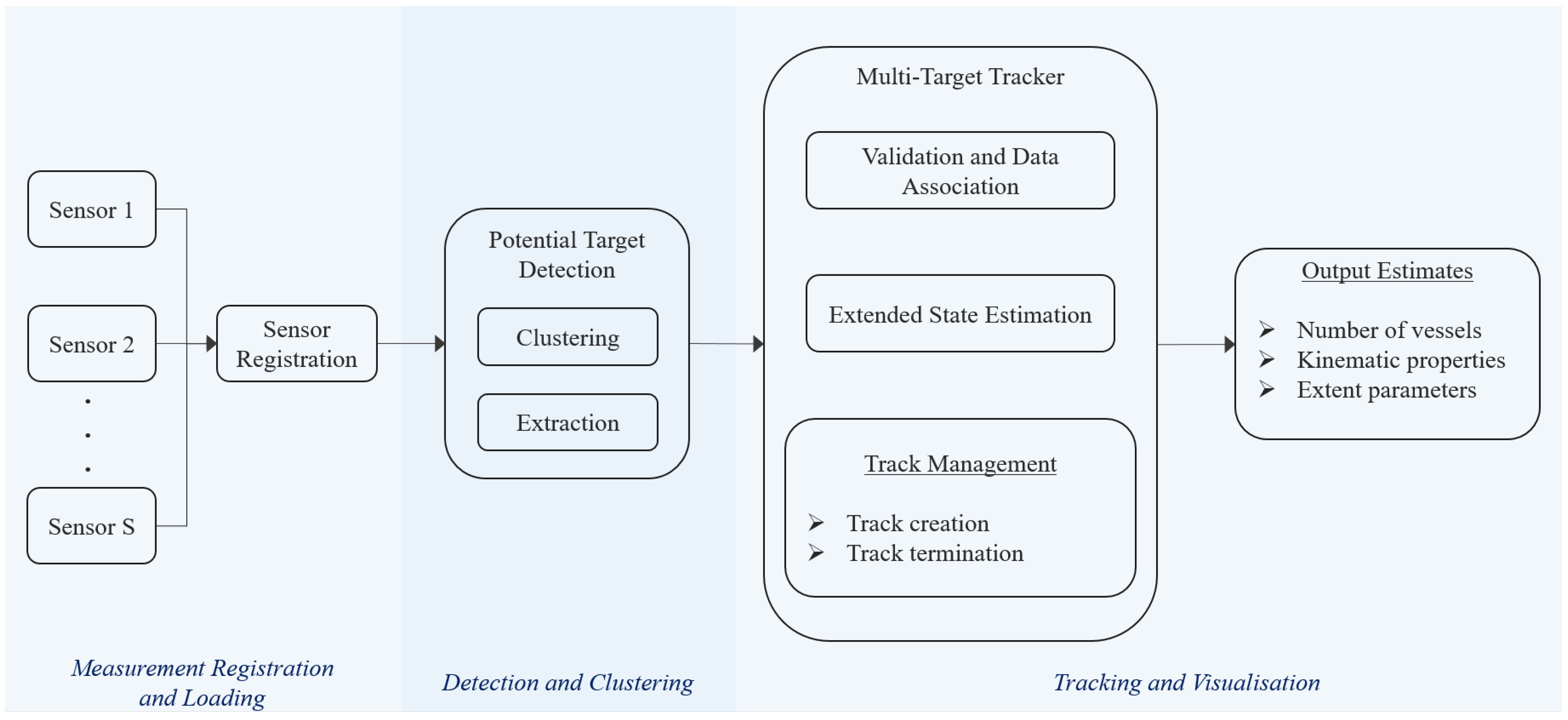
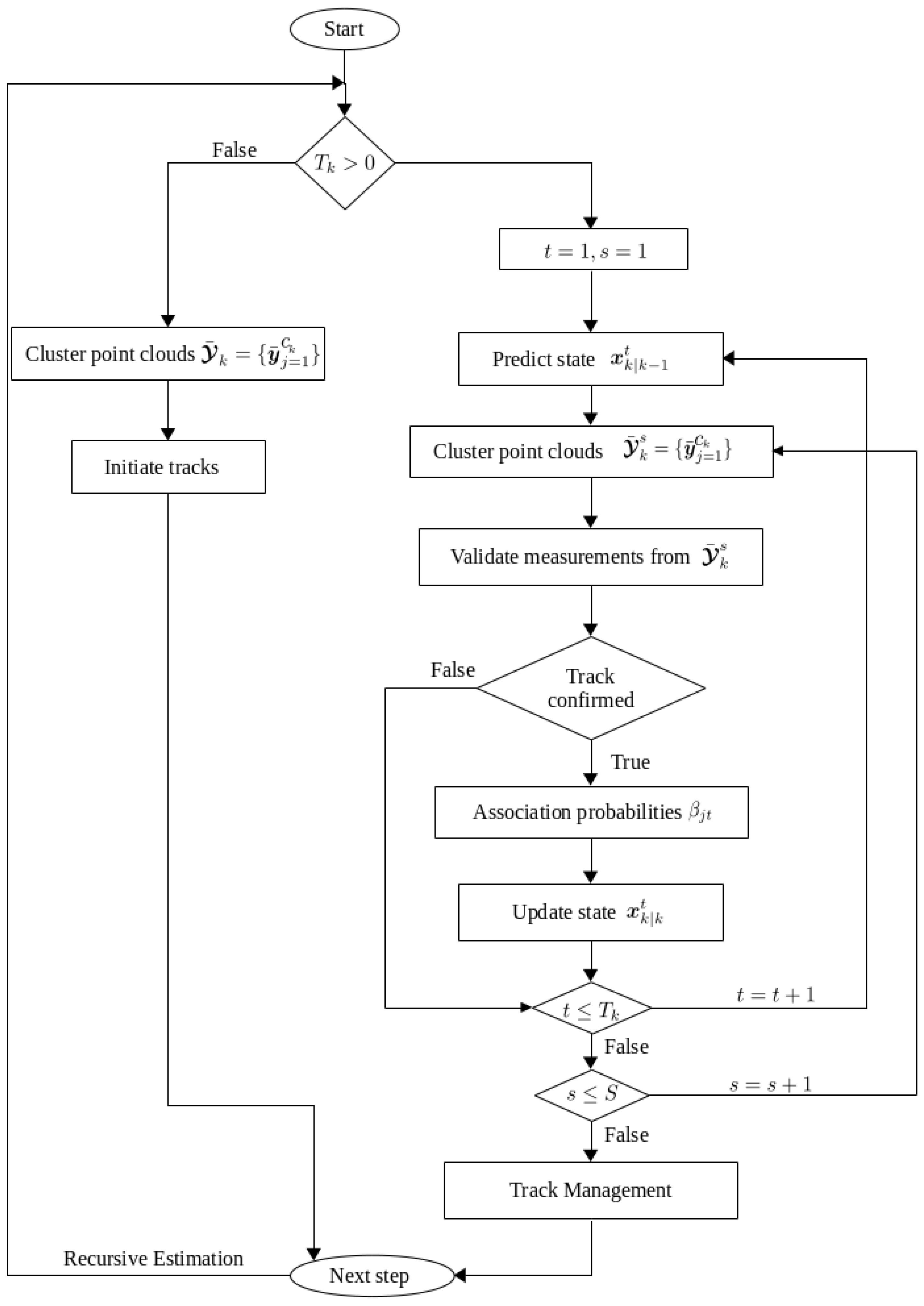
The multitarget set is denoted by ${\mathcal{X}}_k$ at observation step k, such that

$${\mathcal{X}}_k={\left\{{\mathit{x}}_k^t\right\}}_{t=1}^{N_k},$$

(1)

where $N_k$ is the number of confirmed targets, and the individual target state ${\mathit{x}}_k^t$ models the combined properties of interest of vessel t (omitting index t for readability),

$${\mathit{x}}_k={\left[{\mathbf{r}}_k^T,{\mathbf{p}}_k^T\right]}^T.$$

(2)

${(.)}^T$ is the transpose operator. The kinematic state vector is defined as

$${\mathbf{r}}_k={\left[{\mathit{m}}_k^T,{\dot{\mathit{m}}}_k^T\right]}^T,$$

(3)

with its position ${\mathit{m}}_k$ and its velocity vectors ${\dot{\mathit{m}}}_k$. Similarly, the extent state vector is defined by vessel heading ${\alpha }_k\in \left[0,2\pi \right)$, with major-axis ${\ell }_{1,k}$ and minor-axis ${\ell }_{2,k}$, respectively, corresponding to the length and width as

$${\mathbf{p}}_k={\left[{\alpha }_k,{\ell }_{1,k},{\ell }_{2,k}\right]}^T.$$

(4)

The observation region is covered by S sensors. The measurement set, which is defined by ${\mathcal{Y}}_k^s={\{{\mathit{y}}_k^{s,1},\dots ,{\mathit{y}}_k^{s,M_k}\}}_{s=1}^S$, contains $M_k$ measurements from the surfaces of all targets within the observation region, and also includes clutter that is assumed to be uniformly distributed over the region.

The posterior multitarget state is sought to be estimated based on the measurements using the Bayes formula, expressed as follows [40]:

$$p\left({\mathcal{X}}_k|{\mathcal{Y}}_k^S\right)\propto \prod _{s=1}^S\prod _{t=1}^{N_k}p\left({\mathcal{Y}}_k^s|{\mathit{x}}_k^t\right)p\left({\mathit{x}}_{k-1}^t|{\mathcal{Y}}_{k-1}^S\right),$$

(5)

with the likelihood and prior densities of individual target t given by $p\left({\mathcal{Y}}_k^s|{\mathit{x}}_k^t\right)$ and $p\left({\mathit{x}}_{k-1}^t|{\mathcal{Y}}_{k-1}^S\right)$, respectively. From the Chapman–Kolmogorov equation, we can express the prediction target state density, $p\left({\mathit{x}}_k^t|{\mathcal{Y}}_{k-1}^S\right)$, as an integral over step $k-1$ as

$$p\left({\mathit{x}}_k^t|{\mathcal{Y}}_{k-1}^S\right)=\int p\left({\mathit{x}}_k^t|{\mathit{x}}_{k-1}^t\right)p\left({\mathit{x}}_{k-1}^t|{\mathcal{Y}}_{k-1}^S\right)d{\mathit{x}}_{k-1}^t,$$

(6)

where the state transition density is given by $p\left({\mathit{x}}_k^t|{\mathit{x}}_{k-1}^t\right)$. When the new set of measurements is acquired, the prediction combines it based on the likelihood so that the posterior is given by

$$p\left({\mathcal{X}}_k|{\mathcal{Y}}_k^S\right)=\prod _{s=1}^S\prod _{t=1}^{N_k}{\displaystyle \frac{1}{c}}p\left({\mathcal{Y}}_k^s|{\mathit{x}}_k^t\right)\int p\left({\mathit{x}}_k^t|{\mathit{x}}_{k-1}^t\right)p\left({\mathit{x}}_{k-1}^t|{\mathcal{Y}}_{k-1}^S\right)d{\mathit{x}}_{k-1}^t,$$

(7)

with normalization term $c=p\left({\mathcal{Y}}_k^s|{\mathcal{Y}}_{k-1}^S\right)$. In our work, the extended posterior target state conditioned over all past measurements until the current ones, denoted as ${\mathbf{Y}}_k^S$, is expressed based on a Gaussian distribution,

$$p\left({\mathit{x}}_k^t|{\mathbf{Y}}_k^S\right)\approx \mathcal{N}\left({\mathit{x}}_k^t;{\widehat{\mathit{x}}}_k^t,{\mathbf{C}}_k^{\mathit{x}}\right),$$

(8)

where ${\mathit{x}}_k^t$ is the predicted state with zero-mean covariance ${\mathbf{C}}_k^{\mathit{x}}$.

3. Processing Chain

With the objective to solve the METT problem defined above, we propose a dedicated processing chain as shown in Figure 2. The latter is segregated into three main functional blocks explained in the following subsections.

3.1. Measurement Registration and Loading

Data transmitted from multiple cooperative ground radar stations are gathered, decoded, and registered around a common point of reference. For our system, the data are transmitted using the All Purpose Structured EUROCONTROL Surveillance Information Exchange (ASTERIX) [42] protocol.

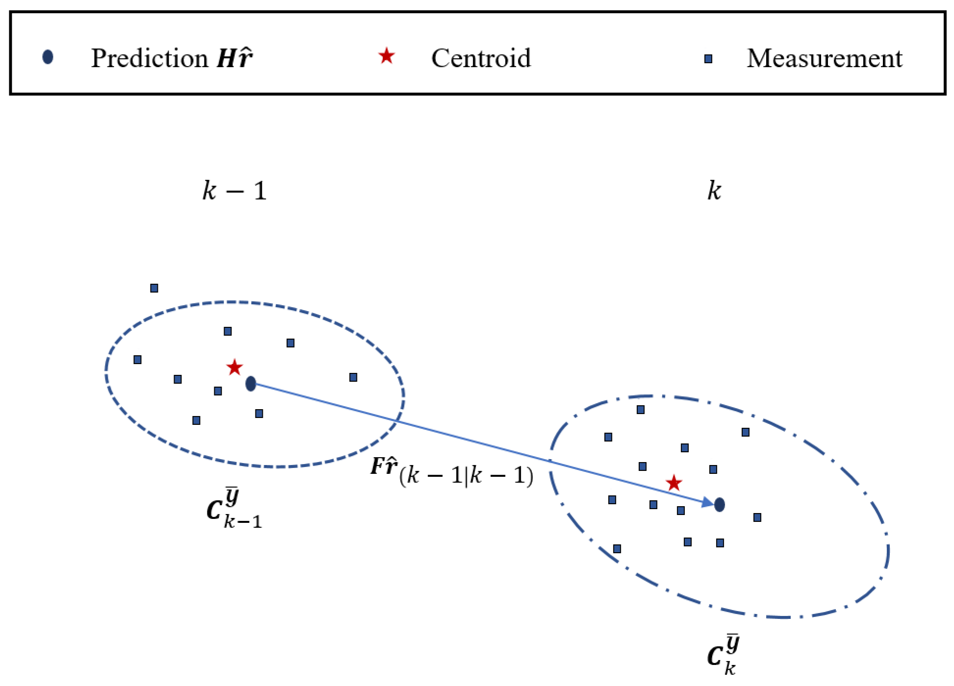
3.2. Detection and Clustering

The radar measurements registered at a single observation step are in the form of point clouds, each cloud often yielding measurements in the order of hundreds, with unknown origins. For instance, the point clouds could have originated from true targets, aids-to-navigation, and clutter formed due to environmental conditions or error sources within the concerned sensor. In order to obtain the potential targets, the measurements are first subjected to a clustering approach while they are being represented in pixel coordinates. The idea is to identify specific clusters within the set of point clouds following the intuition that a point cloud would most likely be originated from one of the abovementioned sources. Clustering is an unsupervised approach and has been commonly implemented by simple methods such as k-means [43], or the Density-based Spatial Clustering of Applications with Noise (DBSCAN) [44], which is less susceptible to spherical distributions and does not need to rely on a predefined number of clusters, as compared to the former [41]. Furthermore, unlike in the former work, the sensor resolution from ground stations is higher, where we can expect a pixel to represent appropriately 1 m.

The clustering step is an important factor affecting the efficiency of the tracking filter overall, as instead of processing every measurement, only the identified clusters that belong to potential targets are processed, to thereby calculate the so-called cluster-to-target association probabilities.

3.3. Tracking and Visualization

At this stage, the clustered measurements are transformed to the local East North Up (ENU)-based coordinates system to model the vessels’ extended states and motions over time within our filter. As the standard JPDA filter assumes a known number of targets, an external track management module for handling target creation and deleting duplicate or out-of-range targets is employed. We note that since our major contribution is, in essence, the application of METT on ASTERIX radar data, we use a sequential sensor-update scheme in this work, and the use of more complex topologies is considered out of scope.

The estimates are finally projected back on the video stream or the specific user interface, where the tracked vessels’ elliptical approximations are directly displayed. Screenshots of the system shall be provided in Section 5.

4. The PAKF-JPDA Filter for METT

This section presents our filter for METT, based on [40], by describing the motion and measurement models, the adaptive validation step, and the elliptical model involved in the overall tracker itself.

Let ${\overline{\mathcal{Y}}}_k^s={\{{\overline{\mathit{y}}}_k^{s,1},\dots ,{\overline{\mathit{y}}}_k^{s,C_k}\}}_{s=1}^S$ denote the set of all $C_k$ clusters, defined by their respective centroids $\overline{\mathit{y}}$, and the set ${\overline{\mathcal{Y}}}_{k-1}^S$ denote all the measurements up until $k-1$ from all cooperating sensors. Rewriting the previous definition in (5), the posterior is expressed as [40]

$$p\left({\mathcal{X}}_k|{\overline{\mathcal{Y}}}_k^S\right)\propto \prod _{s=1}^S\prod _{t=1}^{N_k}p\left({\overline{\mathcal{Y}}}_k^s|{\mathit{x}}_k^t\right)p\left({\mathit{x}}_{k-1}^t|{\overline{\mathcal{Y}}}_{k-1}^S\right),$$

(9)

since the multitarget state is now directly conditioned over the centroids, where $C_k\le M_k$ ideally holds at every step.

The concept adopted for the filter is shown in Figure 3, with an aim to optimize the estimation process by the association of a cluster to a particular target. The spread of a respective cluster is accounted for in the validation and association steps, and is eventually used to extract elliptical measurements based on an EVD approach to update the extent parameters.

4.1. Motion Model

The target kinematic state is assumed to temporally evolve based on an Nearly Constant Velocity (NCV) model [45], while the target parameter vector evolves based on a standard linear model to adapt for vessel extent changes over time and are each (omitting the target index) given by

$$\begin{array}{cc}\hfill {\mathbf{r}}_k& ={\mathbf{F}}_{\mathbf{r}}{\mathbf{r}}_{k-1}+{\omega }_{k-1}^{\mathbf{r}},\hfill \end{array}$$

(10)

$$\begin{array}{cc}\hfill {\mathbf{p}}_k& ={\mathbf{F}}_{\mathbf{p}}{\mathbf{p}}_{k-1}+{\omega }_{k-1}^{\mathbf{p}},\hfill \end{array}$$

(11)

where

• transition matrices ${\mathbf{F}}_{\mathbf{r}}=\left[\begin{array}{c}10T0\\ 010T\\ 0010\\ 0001\end{array}\right]$ with observation interval T and ${\mathbf{F}}_{\mathbf{p}}={\mathbf{I}}_3$, ${\mathbf{I}}_3$ denoting the identity matrix of dimension 3;
• ${\omega }_{k-1}^{\left(•\right)}$ are the vector-respective additive zero-mean Gaussian noises with covariances ${\mathbf{C}}_{\left(•\right)}^{\omega }$.

The overall target’s dynamic uncertainties are accounted for by their respective covariances ${\mathbf{C}}_k^{\mathbf{r}}$ and ${\mathbf{C}}_k^{\mathbf{p}}$ as follows:

$$\begin{array}{cc}\hfill {\mathbf{C}}_k^{\mathbf{r}}& ={\mathbf{F}}_{\mathbf{r}}{\mathbf{C}}_{k-1}^{\mathbf{r}}{\left({\mathbf{F}}_{\mathbf{r}}\right)}^T+{\mathbf{C}}_{\mathbf{r}}^{\omega },\hfill \end{array}$$

(12)

$$\begin{array}{cc}\hfill {\mathbf{C}}_k^{\mathbf{p}}& ={\mathbf{F}}_{\mathbf{p}}{\mathbf{C}}_{k-1}^{\mathbf{p}}{\left({\mathbf{F}}_{\mathbf{p}}\right)}^T+{\mathbf{C}}_{\mathbf{p}}^{\omega },\hfill \end{array}$$

(13)

4.2. Measurement Model

The centroid ${\overline{\mathit{y}}}^j$ of clustered point cloud j, assumed to be distributed over the target’s surface, is modeled as a perturbation by zero-mean additive Gaussian noise ${\mathit{v}}^{\mathbf{r}}$ with covariance ${\mathbf{C}}_{\mathbf{r}}^{\mathit{v}}$. Omitting the sensor indices, the linear measurement model is defined as [40]

$${\overline{\mathit{y}}}_k^j=\underset{:={\widehat{\mathit{y}}}_k^{\mathbf{r}}}{\underbrace{{\mathbf{H}}_{\mathbf{r}}{\mathbf{r}}_k^t}}+{\mathit{v}}_k^{\mathbf{r}},$$

(14)

where ${\mathbf{H}}_{\mathbf{r}}={\left[{\mathbf{I}}_2,{\mathbf{0}}_2\right]}^T$ is the measurement matrix. We denote the predicted centroid of the target by ${\widehat{\mathit{y}}}_k^{\mathbf{r}}$.

The measurement model for the extent parameter vector follows a similar model, where the extent parameters are also assumed to be corrupted with Gaussian noise [40]:

$${\mathit{y}}_k^{p,j}={\mathbf{H}}_{\mathbf{p}}{\mathbf{p}}_k^t+{\mathit{v}}_k^{\mathbf{p}},$$

(15)

where ${\mathbf{H}}_{\mathbf{p}}={\mathbf{I}}_3$ and the measurement noise covariance ${\mathbf{C}}_{\mathbf{p}}^{\mathit{v}}$ consists of user-defined values to account for uncertainty in the measurement. The generation of measurement vector ${\mathit{y}}_k^{\mathbf{p},j}$ for updating the extent parameters is explained within the scope of our PAKF algorithm in Section 4.5.

4.3. Validation

In order to establish an initial association between a centroid and its potential source, a validation scheme is adopted with an adaptive gating approach. The centroid validity is first checked based on target t’s ellipsoidal gate as follows:

$${\left({\overline{\mathit{y}}}_k^j-{\widehat{\mathit{y}}}_k^{\mathbf{r}}\right)}^T{\left({\mathbf{C}}_k^{\overline{\mathit{y}},t}\right)}^{-1}\left({\overline{\mathit{y}}}_k^j-{\widehat{\mathit{y}}}_k^{\mathbf{r}}\right)\le \gamma ,$$

(16)

where ${\widehat{\mathit{y}}}_k^{\mathbf{r}}$ is the prediction, $\gamma$ is the gating threshold, and ${\mathbf{C}}_k^{\overline{\mathit{y}},t}$ is the innovation covariance. The latter is calculated as [41,46]

$${\mathbf{C}}_k^{\overline{\mathit{y}},t}={\mathbf{H}}_{\mathbf{r}}{\mathbf{C}}_k^{\mathbf{r},t}{\left({\mathbf{H}}_{\mathbf{r}}\right)}^T+{\mathbf{C}}_{\mathit{r}}^{\mathbf{v}}+{\mathbf{C}}_{k-1}^{\mathbf{D},t},$$

(17)

with dispersion matrix ${\mathbf{C}}_{k-1}^{\mathbf{D},t}$ intuitively accounting for the target’s extent by the spread of the measurements within the cluster in a two-dimensional space. The method is originally based on our previous work [41], with the modification to now directly consider all of the particular cluster members without additional gating for efficiency.

Therefore, at step k, the dispersion matrix obtained from the previous step is used in the calculation of the innovation covariance as given in (17). This process can be visualized in Figure 4, where we omitted target index for readability. For every validated centroid, the dispersion of the corresponding cluster is then recalculated to be used in the next step, thus gradually adapting the gate to changes in the target extent.

4.4. Association Probabilities

Given the posterior definition from (9), the density of a target-specific posterior $p\left({\mathit{x}}_k^t\right)$ can be represented as an approximation weighted by the marginal association probabilities $\beta$ as follows [40]:

$$p\left({\mathit{x}}_k^t\right)\approx \sum _{j=1}^{C_k}{\beta }_{jt}^{s}p\left({\mathit{x}}_k^t|{\overline{\mathit{y}}}_k^{s,j}\right).$$

(18)

${\beta }_{jt}^s$ is the probability that centroid ${\overline{\mathit{y}}}_k^{s,j}$ recorded from sensor s has originated from t and is computed from the following [41,47]:

$${\beta }_{jt}^s=\left\{\begin{array}{c}\mathcal{N}\left({\overline{\mathit{y}}}_j;{\widehat{\mathit{y}}}_k^{\mathit{r}},{\mathbf{C}}_k^{\overline{\mathit{y}},t}\right)\mathrm{if}\mathrm{origin}\mathrm{is}\mathrm{a}\mathrm{target},\hfill \\ V^{-1}\mathrm{otherwise}\mathrm{clutter}.\hfill \end{array}\right.$$

(19)

The volume of the validation region is defined as in [47]:

$$V=n_{\mathit{y}}\left({\gamma }^{n_{\mathit{y}}/2}\right)\sqrt{|{\mathbf{C}}_k^{\overline{\mathit{y}},t}|},$$

(20)

where $n_{\mathit{y}}$ is the dimension of the measurement (2 in our case), and $\gamma$ corresponds to the threshold. Clutter within the observation region is assumed to be spatially (Poisson) distributed. For a more detailed review of the equations, our previous work can be referred to [41].

4.5. PAKF for Extent Estimation

The PAKF approach was introduced in [16], where the dispersion matrix of a point cloud was used to generate the measurement vector ${\mathit{y}}^{\mathbf{p}}$ for updating the extent parameters in $\mathbf{p}$. In essence, the dispersion matrix of a cluster with centroid ${\overline{\mathit{y}}}_k$ comprising d number of points is given by the following:

$$\begin{array}{cc}\hfill {\mathbf{C}}^D& =\frac{1}{d-1}\sum _{i=1}^d\left({\mathit{y}}_k^i-{\overline{\mathit{y}}}_k\right){\left({\mathit{y}}_k^i-{\overline{\mathit{y}}}_k\right)}^T,\hfill \end{array}$$

(21)

$$\begin{array}{cc}\hfill & =\left[\begin{array}{c}{\sigma }_e^2{\sigma }_{en}^2\\ {\sigma }_{en}^2{\sigma }_n^2\end{array}\right],\hfill \end{array}$$

(22)

where the subscripts e and n represent the east and north axes, respectively. Under the assumption and constraint of positive definiteness, ${\mathbf{C}}^D$ can be expressed in terms of ${\mathit{y}}^{\mathbf{p}}=[a,b,\theta ]$ based on the following relationship:

$${\mathbf{C}}^D=\mathcal{R}\left(\theta \right)\left(\begin{array}{c}{a}^{2}0\\ 0b^2\end{array}\right)\mathcal{R}{\left(\theta \right)}^T,$$

(23)

with rotation matrix $\mathcal{R}\left(\theta \right)$ and length of the semi-axes $ab$ and b. By accounting for the measurement noise and applying EVD, the extent measurements can be thus extracted from the validated clusters. The algorithm for the updates, taken from [16], is provided in

Table 1. Elliptical principal axes model updates, adapted with permission from [16] ©2021 IEEE.

Updating Kinematic Parameters
${\mathit{y}}_k^{\mathbf{r}}:={\overline{\mathit{y}}}_k=\frac{1}{d_k}{\sum }_{i=1}^{d_k}{\mathit{y}}_k^i$
${\widehat{\mathit{y}}}_k^{\mathbf{r}}={\mathbf{H}}_{\mathbf{r}}{\widehat{\mathbf{r}}}_{k|k-1}$
${\mathbf{C}}_k^{\mathbf{r}\mathit{y}}=$${\mathbf{C}}_{k|k-1}^{\mathbf{r}}{\mathbf{H}}_{\mathbf{r}}^T$
${\mathbf{C}}_k^{\mathit{yy}}={\mathbf{H}}_{\mathbf{r}}{\mathbf{C}}_{k|k-1}^{\mathbf{r}}{\mathbf{H}}_{\mathbf{r}}^T+{\mathbf{C}}_{\mathbf{r}}^{\upsilon }$
${\widehat{\mathbf{r}}}_{k|k}={\widehat{\mathbf{r}}}_{k|k-1}+{\mathbf{C}}_k^{\mathbf{r}\mathit{y}}{\left({\mathbf{C}}_k^{\mathit{yy}}\right)}^{-1}\left({\mathit{y}}_k^{\mathbf{r}}-{\widehat{\mathit{y}}}_k^{\mathbf{r}}\right)$
${\mathbf{C}}_{k|k}^{\mathbf{r}}={\mathbf{C}}_{k|k-1}^{\mathbf{r}}-{\mathbf{C}}_k^{\mathbf{r}\mathit{y}}{\left({\mathbf{C}}_k^{\mathit{yy}}\right)}^{-1}{\left({\mathbf{C}}_k^{\mathbf{r}\mathit{y}}\right)}^T$
Extent Measurements Extraction through EVD
${\mathbf{C}}^D=\frac{1}{d_k-1}{\sum }_{i=1}^{d_k}\left({\mathit{y}}_k^i-{\overline{\mathit{y}}}_k\right){\left({\mathit{y}}_k^i-{\overline{\mathit{y}}}_k\right)}^T$
${\mathbf{C}}^{\widehat{D}}={\mathbf{C}}^D-{\mathbf{C}}_{\mathbf{r}}^{\upsilon }$
$\left[\mathbf{V},{\lambda }_k\right]=\mathtt{eig}\left({\mathbf{C}}^{\widehat{D}}\right)$
${[{\lambda }_1,{\lambda }_2]}^T=\mathtt{diag}\left({\lambda }_k\right)$
${[a_k,b_k]}^T=\sqrt{{\left[{\lambda }_1,{\lambda }_2\right]}^T}$
${\theta }_k=\mathtt{atan}\mathtt{2}\left(\frac{{\mathrm{v}}_{1,\left(n\right)}}{{\mathrm{v}}_{1,\left(e\right)}}\right)$
Updating Extent Parameters
${\mathit{y}}_k^{\mathbf{p}}:=\left[{\theta }_k,a_k,b_k\right]$
${\widehat{\mathit{y}}}_k^{\mathbf{p}}={\mathbf{H}}_{\mathbf{p}}{\widehat{\mathbf{p}}}_{k|k-1}$
${\mathbf{C}}_k^{\mathbf{p}\mathit{y}}={\mathbf{C}}_{k|k-1}^{\mathbf{p}}{\mathbf{H}}_{\mathbf{p}}^T$
${\mathbf{C}}_k^{\mathit{yy}}={\mathbf{H}}_{\mathbf{p}}{\mathbf{C}}_{k|k-1}^{\mathbf{p}}{\mathbf{H}}_{\mathbf{p}}^T+{\mathbf{C}}_{\mathbf{p}}^{\upsilon }$
${\widehat{\mathbf{p}}}_{k|k}={\widehat{\mathbf{p}}}_{k|k-1}+{\mathbf{C}}_k^{\mathbf{p}\mathit{y}}{\left({\mathbf{C}}_k^{\mathit{yy}}\right)}^{-1}\left({\mathit{y}}_k^{\mathbf{p}}-{\widehat{\mathit{y}}}_k^{\mathbf{p}}\right)$
${\mathbf{C}}_{k|k}^{\mathbf{p}}={\mathbf{C}}_{k|k-1}^{\mathbf{p}}-{\mathbf{C}}_k^{\mathbf{p}\mathbf{y}}{\left({\mathbf{C}}_k^{\mathit{yy}}\right)}^{-1}{\left({\mathbf{C}}_k^{\mathbf{p}\mathit{y}}\right)}^T$

.

In principle, the angular quantities are corrected at two steps. The first step is performed right before updating the extent parameters: since the four quadrant inverse tangent function $\mathtt{atan}\mathtt{2}$ returns $\theta$ values in $\left[-\pi ,\pi \right]$, $2\pi$ is added to the negative values to conform to an interval of $\left[0,2\pi \right]$. The second step, independent of the filtering equations, involves shifting the final orientation estimate ${\alpha }_k$ by $\pi /2$ to maintain a north-up heading. The heading estimates in our algorithm are assumed to be uncoupled and unaligned from the vessel kinematics due to the vessel’s current-based drifting propensities. As such, we explain how the heading estimates are presented further in Section 5.

4.6. Track Management and Fusion

Since the standard JPDA assumes a known number of targets, the current approach was developed to account for estimating varying numbers of targets by the implementation of a separate track management module. The latter is in charge of track initiation, confirmation, and deletion, based on the $M/N$ rule. For instance, every unassociated centroid is treated as a potential target (initiation) which shall be confirmed upon M successful validations over N continuous observation steps.

A target is deleted in two situations; when there are no longer further validations over a number of steps and in the case of track duplication, either the older track is retained (for example, if $T_k$ exceeds a predefined limit), or the tracks are fused according to the standard fusion approach in the work of Singer and Kanyuck [48].

An outline of the steps involved in our combined PAKF-JPDA filter can be found in Figure 5 below.

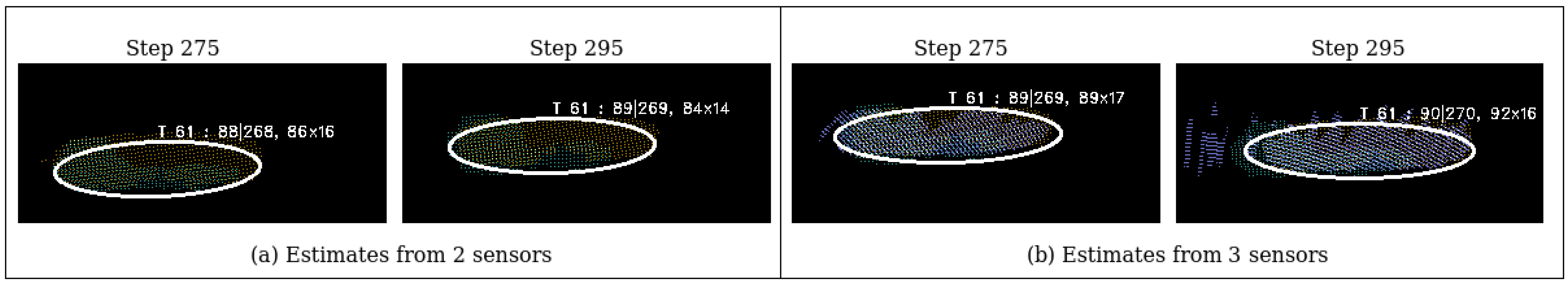
5. Application and Results

This section explains the setup of the port region from where the radar streaming was recorded in a real-world setting, and provides the results of the detection and tracking algorithms.

5.1. Real-World Radar Streaming

Participating ground stations stream their radar detections from the Port of Hamburg over the ASTERIX protocol. The stations overlooking the region are located in the north, northeast, and south directions along the banks of the river Elbe. The sampling is at every $2.5$ s for all sensors. Furthermore, the sensors have the advantage of providing views from at least 30 m above the ground.

5.2. Clustering

In the detection step, we applied the DBSCAN algorithm with the $eps$ parameter set at 20, while the minimum number of detection points $min\_samples$ to obtain a valid cluster was taken to be 50. The parameters were tuned on a trial-and-error basis with consideration given to the prevailing environmental conditions to ensure that the clusters were neither over- nor underfitted.

For illustrative purposes, we present exemplar sensor-wise clustering results as well as the overlaid measurements from a random step in Figure 6. The port structure, visible from the figure, is masked out in our process for efficiency, so that only detections from the extracted waterway are subject to DBSCAN. The centroids are then converted from image coordinates to the local ENU coordinates before they are processed by our tracker.

In our work, the value for $eps$ was set so as to maximize the likelihood that at most one cluster per vessel is obtained. This factors in the possibility that measurements could be denser over some parts of the vessel. A lower $eps$ value could yield multiple clusters originating from the same vessel, which would have challenged our tracker in the next phase. With regard to the second parameter, any value within the range $45<min\_samples<60$ would yield almost the same number of clusters as long as the external conditions remained unchanged. Values below the lower limit would, however, result in more clusters, including those of clutter measurements with an increase in processing time, while values beyond the upper limit could result in failure to detect potential vessels.

5.3. Multisensor METT Visualization

Detections from Sensor 1, based upon our experience, were the most reliable in terms of target detectability and coverage among the other two, and centroids yielded from them were used for track initiation at the start. Henceforth, centroids from the remaining sensors were also used in track initiation. As Sensor 3’s detections were noisiest and yielded occasional radar reflections and backscattering effects, they were given less certainty. The relevant parameter settings for our clustering and tracking approaches are given in

Table 2. Parameter settings and description.

Parameter	Value	Description
$eps$	20	$eps$ value for DBSCAN in pixels
$min\_samples$	50	Minimum number of pixel points for DBSCAN
${\mathbf{C}}_k^{\mathbf{r}}$	$\mathtt{diag}(2^2,2^2,3^2,3^2)$	Kinematic state covariance at initiation step k, [m, m, km/h, km/h]
${\mathbf{C}}_k^{\mathbf{p}}$	$\mathtt{diag}({0.25}^2,1^2,1^2)$	Extent state covariance at initiation step k, [${}^{\mathrm{o}}$, m, m]
${\mathbf{C}}_{\mathbf{r}}^{\omega }$	$\mathtt{diag}({20}^2,{20}^2,{0.2}^2,{0.2}^2)$	Kinematic state process noise, [m, m, km/h, km/h]
${\mathbf{C}}_{\mathbf{p}}^{\omega }$	$\mathtt{diag}({0.5}^2,{0.2}^2,{0.1}^2)$	Extent state process noise, [${}^{\mathrm{o}}$, m, m]
${\mathbf{C}}_{\mathbf{r}}^{\upsilon ,1}$	$\mathtt{diag}(2^2,2^2)$	Measurement noise for Sensor 1 in meters
${\mathbf{C}}_{\mathbf{r}}^{\upsilon ,2}$	$\mathtt{diag}(3^2,3^2)$	Measurement noise for Sensor 2 in meters
${\mathbf{C}}_{\mathbf{r}}^{\upsilon ,3}$	$\mathtt{diag}(6^2,6^2)$	Measurement noise for Sensor 3 in meters
${\mathbf{C}}_{\mathbf{p}}^{\upsilon }$	$\mathtt{diag}(5^2,{0.5}^2,{0.5}^2)$	Measurement noise for extent parameters, [${}^{\mathrm{o}}$, m, m]
$\gamma$	$9.21$	Gate threshold
$M/N$	$5/6$	Track confirmation condition
$M^{-}/N^{-}$	$4/4$	Track termination condition

.

The estimated vessel extent parameters, including its identification number that is assigned at the time of initialization, are directly printed in our application, while the kinematic ones are internally stored. Since orientation of ellipses can be ambiguous, we consider two possibilities based on the velocity of a vessel. The typical annotation format, with respect to (4), is as follows:

$$T\#:\underset{\mathrm{orientation}}{\underbrace{{\alpha }_k^t|{\tilde{\alpha }}_k^t}},\underset{\mathrm{length}\times \mathrm{width}}{\underbrace{2{\ell }_{1,k}^t\times 2{\ell }_{2,k}^t}},$$

(24)

where

• # is the step at which the target was initialized.
• Orientation values from ${\alpha }_k^t|{\tilde{\alpha }}_k^t$ for two possibilities: when vessel navigates from west to east, its heading is taken as ${\alpha }_k^t$, and in the opposite case, the heading is taken as ${\tilde{\alpha }}_k^t={\alpha }_k^t+\pi$.
• $2{\ell }_{1,k}^t\times 2{\ell }_{2,k}^t$ represent the length and width, respectively.

6. Discussion

In this section, we present some discussion of our work regarding two aspects. At first, we focus on the current framework and then on the framework’s potential for further development.

6.1. Performance of Current Framework

Given the availability of the Automatic Identification System (AIS) information during the recorded time, we illustrate the validity of our tracker’s results. In Figure 7, the dimensions of four types of vessels are shown against their references: a passenger ship, cargo, tug, and tanker, respectively. We focus on the performance of tracking with varying sensor combinations, in which case we show results from two sensors (Sensors 1 and 2) as well as results from all sensors.

Most of the vessels’ estimations in Figure 7 were within 5 m of their references when we considered the combination of the best two sensors. The results show that estimates in principle depend on the coverage, measurement quality, and sensor synchrony, which are the factors discussed next. At the time of track initialization, the size estimates are smaller as they are only partially visible within the observation region before converging closer to their true values when fully visible. The same is applicable as a vessel moves away from the observation region. This behavior was captured by the passenger ship as it navigated through the region. For the other vessels, the plots’ axes were limited for the period until, and as long as, the vessels were fully visible.

While vessel dimensions are based on their hulls, radar reflections also arise due to the vessel’s superstructure and the onboard objects. Hence, in our case, the width was most likely to deviate from the reference, given the positioning of the ground stations. As the three-sensors combination included noisier measurements from Sensor 3, we found their fused estimates to be less accurate in general despite accounting for Sensor 3’s uncertainty. To better demonstrate this, we consider the example provided in Figure 8, where the extents of the cargo vessel are shown at the same observation steps under different sensor combinations. An interpretation of the printed values from the leftmost figure would be that the vessel is a size of approximately 86 m by 16 m and was being tracked over its trajectory as it headed ${88}^{\circ }$ (deduced based on cumulative previous steps) from the north across the region. In addition to the aforementioned width deviation, the length estimates are closer to the reference for the two-sensors combination. In contrast, the length estimates were affected by the reflections of Sensor 3, and had a tendency to therefore be larger than the true value.

Regarding the last factor, there are cases of occasional sensor asynchrony which may lead to overestimation of both extent and kinematic properties when persistent. Some examples are depicted in Figure 9 over four consecutive frames. The individual row shows the effect of having asynchronous measurements at a point of time and how the filter continues. For most cases, the estimates remain close to their true values, even if there is interference from a combination of the three factors.

Finally, we look at the fused estimates over the entire observation region for an MTSAM application as a whole on the basis of snapshots taken at two random observation steps in Figure 10 and Figure 11. In Figure 10, there was a single vessel underway. Its estimated size was 65 m by 16 for an AIS-based reference size of 56 m by 12 owing to the trails and reflections. However, due to the persistent reflections from Sensor 3, a ghost vessel (false positive) was generated towards the east. Similar to all false positives in our case, the latter track lingered for some steps before being terminated.

From the results in Figure 11, which shows five vessels and a ghost vessel, an essential point can be noted. The clustering algorithm was more sensitive to radar reflections (see vessel T103) than to water trails (see vessel T110), as detections resulting from the latter are relatively sparser, thus not meeting requirements for being a cluster (under our chosen parameters). When we look closer at the two vessels T61 and T105 in the lower sides of the main waterway in the figure, there was limited coverage for Sensor 3 as most measurements belonged to either Sensor 1 or to Sensor 2. On the other hand, despite being the noisiest among the three sensors, Sensor 3 was the only one which covered the southern part of the observation region completely, while the other two sensors had limited coverage there. This is the core reason why our algorithm could still initiate tracks based on the noisy reflections from Sensor 3, and it therefore remains a challenge to eliminate ghost vessels born from it.

Nonetheless, our system was able to so far successfully track the extended states of multiple dynamic vessels continuously. The computation time of one observation step was recorded as $1.98$ s, with the streaming being processed on a $2.60$ GHz Intel Quad Core processor system, employing PyCharm 2019 with Python version $3.6$. Measurement loading accounted for $35\%$ of the entire processing time, and clustering accounted for $34\%$, with the remaining accounting for our tracker.

6.2. Advancing the Framework

Our planned direction for developing the framework’s abilities would focus on accuracy and computational time optimization. Instead of homogeneous radar platforms, irrespective of whether the sensors are static (as they were in this work) or dynamic, the framework shall cater for heterogeneous platforms that include sensors such as the AIS, or Light Detection and Ranging (lidar). The current framework can easily accommodate AIS, which would require similar steps for coordinate conversion and fusing the measurements for estimating the kinematic positions. On the other hand, lidar measurements are restricted to close-range targets and often have limited perspective. Yet, they could aid the extent estimation, although specific strategies would be required within the framework to account for them. Despite the scope, challenges such as sensor synchronization shall remain, and adequate trade-offs would have to be considered depending on the situation at hand and requirements as well. The contrast can be stated as follows: radar–lidar fusion can provide more accurate estimations to assist vessels turning around or berthing in harbors, while AIS–radar fusion would be more suitable to obtain reliable and robust traffic situation.

7. Conclusions

The two main contributions of this work are a framework for processing ASTERIX-based detections from radar streams and the application and evaluation of an elliptical METT algorithm, the PAKF-JPDA, to estimate the kinematic and extent parameters of an unknown, dynamic number of vessels in a multisensor harbor setting. The framework defines the functional steps involved from measurement loading to target tracking, thus enabling vessel traffic monitoring and aiding situation assessment, for instance, during vessel turns in sensitive regions within harbors. Methods for coordinate conversion and clustering were applied on measurements from three high-resolution radar sensors before our tracker estimated the position, velocity, size, and orientation of potential vessels from the resulting fused measurements.

We demonstrated the framework based on radar video streaming. Snapshots of the results with different sensor combinations were presented, and for further analysis, four types of vessels, namely, passenger ship, cargo, tug, and tanker, were compared against their AIS-based references to highlight the accuracy as well as possible sensitivity of the sensors. The elliptical extent estimates were directly projected into the stream for visualization, and our approach was able to track multiple vessels in the presence of clutter, water trails, and radar reflections, despite some false positives lingering for some continuous steps before being terminated.

For the outlook, we plan to investigate the heterogeneous expansion of our framework by fusing measurements from both static and dynamic radars with other sensors such as the AIS-broadcast information and potentially lidars for closer ranges. Furthermore, we also plan on improving the system’s vessel detection capability both in terms of accuracy and computational requirements.

References

1. European Maritime Safety Agency (EMSA). Analysis of Marine Casualties and Incidents Involving Container Vessels. In Safety Analysis of EMCIP Data—Container Vessels; European Maritime Safety Agency (EMSA): Lisbon, Portugal, 2020; pp. 8–9. [Google Scholar]
2. Felski, A.; Zwolak, K. The Ocean-Going Autonomous Ship—Challenges and Threats. J. Mar. Sci. Eng. 2020, 8, 41. [Google Scholar] [CrossRef]
3. Singh, S.; Fowdur, J.S.; Gawlikowski, J.; Medina, D. Leveraging Graph and Deep Learning Uncertainties to Detect Anomalous Maritime Trajectories. IEEE Trans. Intell. Transp. Syst. 2022, 23, 23488–23502. [Google Scholar] [CrossRef]
4. Vo, B.N.; Mallick, M.; Bar-Shalom, Y.; Coraluppi, S.; Osborne, R.; Mahler, R. Multitarget Tracking. In Wiley Encyclopedia of Electrical and Electronics Engineering; John Wiley & Sons, Inc.: Hoboken, NJ, USA, 2015; pp. 1–25. [Google Scholar] [CrossRef]
5. Granström, K.; Baum, M. A Tutorial on Multiple Extended Object Tracking. TechRxiv 2022. [Google Scholar] [CrossRef]
6. Feldmann, M.; Franken, D.; Koch, W. Tracking of Extended Objects and Group Targets Using Random Matrices. IEEE Trans. Signal Process. 2011, 59, 1409–1420. [Google Scholar] [CrossRef]
7. Yang, S.; Baum, M. Tracking the Orientation and Axes Lengths of an Elliptical Extended Object. IEEE Trans. Signal Process. 2019, 67, 4720–4729. [Google Scholar] [CrossRef]
8. Kaulbersch, H.; Baum, M.; Willett, P. An EM approach for Contour Tracking based on Point Clouds. In Proceedings of the 2016 IEEE International Conference on Multisensor Fusion and Integration for Intelligent Systems (MFI), Baden, Germany, 19–21 September 2016; pp. 529–533. [Google Scholar] [CrossRef]
9. Petrov, N.; Gning, A.; Mihaylova, L.; Angelova, D. Box Particle Filtering for Extended Object Tracking. In Proceedings of the 15th International Conference on Information Fusion, Singapore, 9–12 July 2012; pp. 82–89. [Google Scholar]
10. Granström, K.; Lundquist, C.; Orguner, U. Tracking Rectangular and Elliptical Extended Targets using Laser Measurements. In Proceedings of the 14th International Conference on Information Fusion, Chicago, IL, USA, 5–8 July 2011; pp. 1–8. [Google Scholar]
11. Baum, M.; Hanebeck, U.D. Extended Object Tracking with Random Hypersurface Models. IEEE Trans. Aerosp. Electron. Syst. 2014, 50, 149–159. [Google Scholar] [CrossRef]
12. Kaulbersch, H.; Honer, J.; Baum, M. A Cartesian B-Spline Vehicle Model for Extended Object Tracking. In Proceedings of the 21st International Conference on Information Fusion (FUSION), Cambridge, UK, 10–13 July 2018; pp. 1–5. [Google Scholar] [CrossRef]
13. Yao, G.; Wang, P.; Berntorp, K.; Mansour, H.; Boufounos, P.; Orlik, P.V. Extended Object Tracking with Automotive Radar Using B-Spline Chained Ellipses Model. In Proceedings of the ICASSP 2021—2021 IEEE International Conference on Acoustics, Speech and Signal Processing (ICASSP), Toronto, ON, Canada, 6–11 June 2021; pp. 8408–8412. [Google Scholar] [CrossRef]
14. Granström, K.; Baum, M.; Reuter, S. Extended Object Tracking: Introduction, Overview, and Applications. J. Adv. Inf. Fusion 2017, 12, 139–174. [Google Scholar]
15. Mihaylova, L.; Carmi, A.; Septier, F.; Gning, A.; Pang, S.; Godsill, S. Overview of Bayesian Sequential Monte Carlo Methods for Group and Extended Object Tracking. Digit. Signal Process. 2014, 25, 1–16. [Google Scholar] [CrossRef]
16. Fowdur, J.S.; Baum, M.; Heymann, F. An Elliptical Principal Axes-based Model for Extended Target Tracking with Marine Radar Data. In Proceedings of the 24th International Conference on Information Fusion (FUSION 2021), Sun City, South Africa, 1–4 November 2021. [Google Scholar] [CrossRef]
17. Vivone, G.; Braca, P.; Granström, K.; Natale, A.; Chanussot, J. Converted Measurements Random Matrix Approach to Extended Target Tracking Using X-band Marine Radar Data. In Proceedings of the 2015 18th International Conference on Information Fusion (Fusion), Washington, DC, USA, 6–9 July 2015; pp. 976–983. [Google Scholar]
18. Brekke, E.; Eidsvik, J. LIDAR Extended Object Tracking of a Maritime Vessel Using an Ellipsoidal Contour Model. In Proceedings of the Symposium Data Fusion, Bonn, Germany, 9–11 October 2018. [Google Scholar]
19. Han, J.; Kim, S.Y.; Kim, J. Enhanced Target Ship Tracking with Geometric Parameter Estimation for Unmanned Surface Vehicles. IEEE Access 2021, 9, 39864–39872. [Google Scholar] [CrossRef]
20. Koch, J.W. Bayesian Approach to Extended Object and Cluster Tracking using Random Matrices. IEEE Trans. Aerosp. Electron. Syst. 2008, 44, 1042–1059. [Google Scholar] [CrossRef]
21. Lan, J.; Li, X.R. Tracking of Extended Object or Target Group Using Random Matrix: New Model and Approach. IEEE Trans. Aerosp. Electr. Syst. 2016, 52, 2973–2988. [Google Scholar] [CrossRef]
22. Lan, J.; Li, X.R. Extended-Object or Group-Target Tracking Using Random Matrix with Nonlinear Measurements. IEEE Trans. Signal Process. 2019, 67, 5130–5142. [Google Scholar] [CrossRef]
23. Thormann, K.; Baum, M. Incorporating Range-Rate Measurements in EKF-based Elliptical Extended Object Tracking. In Proceedings of the IEEE International Conference on Multisensor Fusion and Integration (MFI), Karlsruhe, Germany, 23–25 September 2021; p. 1. [Google Scholar]
24. Govaers, F. On Independent Axes Estimation for Extended Target Tracking. In Proceedings of the 2019 Sensor Data Fusion: Trends, Solutions, Applications (SDF), Bonn, Germany, 15–17 October 2019; pp. 1–6. [Google Scholar] [CrossRef]
25. Thormann, K.; Yang, S.; Baum, M. A Comparison of Kalman Filter-based Approaches for Elliptic Extended Object Tracking. In Proceedings of the IEEE 23rd International Conference on Information Fusion, FUSION 2020, Rustenburg, South Africa, 6–9 July 2020; pp. 1–8. [Google Scholar]
26. Degerman, J.; Wintenby, J.; Svensson, D. Extended Target Tracking using Principal Components. In Proceedings of the 14th International Conference on Information Fusion, Chicago, IL, USA, 5–8 July 2011; pp. 1–8. [Google Scholar]
27. Li, M.; Lan, J.; Li, X.R. Tracking of Elliptical Extended Object with Unknown but Fixed Lengths of Axes. In Proceedings of the 2020 IEEE 23rd International Conference on Information Fusion (FUSION), Rustenburg, South Africa, 6–9 July 2020; pp. 1–8. [Google Scholar] [CrossRef]
28. Tuncer, B.; Özkan, E. Random Matrix Based Extended Target Tracking with Orientation: A New Model and Inference. IEEE Trans. Signal Process. 2021, 69, 1910–1923. [Google Scholar] [CrossRef]
29. Baum, M.; Faion, F.; Hanebeck, U.D. Modeling the Target Extent with Multiplicative Noise. In Proceedings of the 2012 15th International Conference on Information Fusion, Singapore, 9–12 July 2012; pp. 2406–2412. [Google Scholar]
30. Fowdur, J.S.; Baum, M.; Heymann, F. Tracking Targets with Known Spatial Extent Using Experimental Marine Radar Data. In Proceedings of the 22nd International Conference on Information Fusion (FUSION 2019), Ottawa, ON, Canada, 2–5 July 2019. [Google Scholar]
31. Fowdur, J.S.; Baum, M.; Heymann, F. A Marine Radar Dataset for Multiple Extended Target Tracking. In Proceedings of the 1st Maritime Situational Awareness Workshop (MSAW 2019), Lerici, Italy, 8–10 October 2019. [Google Scholar]
32. Vivone, G.; Braca, P. Joint Probabilistic Data Association Tracker for Extended Target Tracking Applied to X-Band Marine Radar Data. IEEE J. Ocean. Eng. 2016, 41, 1007–1019. [Google Scholar] [CrossRef]
33. Yang, S.; Thormann, K.; Baum, M. Linear-Time Joint Probabilistic Data Association for Multiple Extended Object Tracking. In Proceedings of the 2018 IEEE Sensor Array and Multichannel Signal Processing Workshop (SAM 2018), Sheffield, UK, 8–11 July 2018; pp. 6–10. [Google Scholar] [CrossRef]
34. Yang, S.; Wolf, L.; Baum, M. Marginal Association Probabilities for Multiple Extended Objects without Enumeration of Measurement Partitions. In Proceedings of the 23rd International Conference on Information Fusion, Rustenburg, South Africa, 6–9 July 2020. [Google Scholar] [CrossRef]
35. Schuster, M.; Reuter, J.; Wanielik, G. Probabilistic Data Association for Tracking Extended Targets under Clutter using Random Matrices. In Proceedings of the 2015 18th International Conference on Information Fusion (Fusion), Washington, DC, USA, 6–9 July 2015; pp. 961–968. [Google Scholar]
36. Monika Wieneke, W.K. Probabilistic Tracking of Multiple Extended Targets using Random Matrices. In Proceedings of the SPIE Defense, Security, and Sensing, Orlando, FL, USA, 5–9 April 2010; Volume 7698. [Google Scholar] [CrossRef]
37. Vivone, G.; Granström, K.; Braca, P.; Willett, P. Multiple Sensor Bayesian Extended Target Tracking Fusion Approaches Using Random Matrices. In Proceedings of the 2016 19th International Conference on Information Fusion (FUSION), Heidelberg, Germany, 5–8 July 2016; pp. 886–892. [Google Scholar]
38. Vivone, G.; Granström, K.; Braca, P.; Willett, P. Multiple Sensor Measurement Updates for the Extended Target Tracking Random Matrix Model. IEEE Trans. Aerosp. Electron. Syst. 2017, 53, 2544–2558. [Google Scholar] [CrossRef]
39. Thormann, K.; Baum, M. Fusion of Elliptical Extended Object Estimates Parameterized with Orientation and Axes Lengths. IEEE Trans. Aerosp. Electron. Syst. 2021, 57, 2369–2382. [Google Scholar] [CrossRef]
40. Fowdur, J.S. Multiple Extended Target Tracking in Maritime Environment Using Marine Radar Data. Ph.D. Thesis, University of Göttingen, Göttingen, Germany, 2022. [Google Scholar] [CrossRef]
41. Fowdur, J.S.; Baum, M.; Heymann, F. Real-World Marine Radar Datasets for Evaluating Target Tracking Methods. Sensors 2021, 21, 4641. [Google Scholar] [CrossRef] [PubMed]
42. EUROCONTROL. ASTERIX Protocol. Available online: https://www.eurocontrol.int/asterix (accessed on 4 July 2022).
43. Bock, H.H. Origins and Extensions of the k-means Algorithm in Cluster Analysis. J. Electron. D’Histoire Probab. Stat. Electron. Only 2008, 4, 1–18. [Google Scholar]
44. Ester, M.; Kriegel, H.P.; Sander, J.; Xu, X. A Density-Based Algorithm for Discovering Clusters in Large Spatial Databases with Noise. In Proceedings of the Second International Conference on Knowledge Discovery and Data Mining, KDD’96, Portland, OR, USA,, 2–4 August 1996; AAAI Press: Palo Alto, CA, USA, 1996; pp. 226–231. [Google Scholar]
45. Bar-Shalom, Y.; Kirubarajan, T.; Li, X.R. Estimation with Applications to Tracking and Navigation; John Wiley & Sons, Inc.: New York, NY, USA, 2002. [Google Scholar]
46. Blackman, S.S. Multiple-Target Tracking with Radar Applications; Artech House Publishers: Boston, MA, USA, 1986. [Google Scholar]
47. Bar-Shalom, Y.; Daum, F.; Huang, J. The Probabilistic Data Association Filter. IEEE Control Syst. Mag. 2009, 29, 82–100. [Google Scholar] [CrossRef]
48. Singer, R.; Kanyuck, A. Computer Control of Multiple Site Track Correlation. Automatica 1971, 7, 455–463. [Google Scholar] [CrossRef]
Figure 1. Visualization of simple port setting with three ground stations overlooking a region of interest for monitoring vessel traffic.
Remotesensing 15 02503 g001
Figure 2. Processing chain depicting the main steps in our MTSAM system.
Remotesensing 15 02503 g002
Figure 3. Overview of cluster-to-target association concept for METT. In (i), the black squares represent unassociated measurements from the observation region. Step (ii) depicts the measurements being partitioned into colour-coded clusters, as well as measurements that could be clutter (these remain black). In Step (iii), ellipses represent the estimates of the targets, obtained from cluster-to-target association probabilities.
Remotesensing 15 02503 g003
Figure 4. Validating cluster measurements for the calculation of C k D . A target is shown with a sample previous and current measurements at k 1 and k, respectively, including its positional predictions. At first, the centroid is validated using ellipsoidal gate based on the target’s innovation covariance C k 1 y ¯ , visualized by the dashed ellipse at k 1 . Following this, the measurements belonging to the respective cluster are employed to obtain the next C k D , which is added to the innovation covariance C k y ¯ (ellipse at k) for the adaptive gating at k, and so on.
Remotesensing 15 02503 g004
Figure 5. PAKF-JPDA filter summarized in the flowchart, reprinted with permission from [40] ©2022 University of Göttingen eDiss.
Remotesensing 15 02503 g005
Figure 6. Sample clustering output at a random step. (a) Detections from all the three sensors plotted together, where orange, teal, and purple colors correspond to Sensor 1, Sensor 2, and Sensor 3, respectively. (bd) The final clustering results from each sensor. Colored clusters with their centroids denoted by black crosses ‘×’. Black clusters are considered as noise.
Remotesensing 15 02503 g006
Figure 7. Estimates of four types of vessels from different sensor combinations (solid blue and green lines) against their AIS-based reference values (dotted red lines), with their standard deviations.
Remotesensing 15 02503 g007
Figure 8. Estimates of the cargo with different sensor combinations. The three-sensors combination shows length estimates affected by noisy reflections (Sensor 1: orange, Sensor 2: teal, Sensor 3: purple).
Remotesensing 15 02503 g008
Figure 9. Examples of sensor asynchrony shown in consecutive frames. Each row corresponds to some target(s), the estimated extent(s), and the likely value for estimated orientation is underlined among the extent parameters. Together with sensor asynchrony, water trails and clutter can be observed particularly in rows (ac) (Sensor 1: orange, Sensor 2: teal, Sensor 3: purple). In row (d), we see a two vessels, of which one is making a turn and notice the sensor asynchrony in Frame i + 2 .
Remotesensing 15 02503 g009
Figure 10. Estimates of vessel T0 amid noisy measurements, including reflections due to water trails. T14 in the east is a false positive resulting from noisy radar reflections of Sensor 3 (Sensor 1: orange, Sensor 2: teal, Sensor 3: purple).
Remotesensing 15 02503 g010
Figure 11. Estimates from one vessel and a ghost vessel in the east (result of radar reflections) (Sensor 1: orange, Sensor 2: teal, Sensor 3: purple).
Remotesensing 15 02503 g011