Abstract
Millimeter-wave-based extended target tracking has attracted extensive interest recently because of its privacy, high precision, and low cost. This paper concentrated on crowded indoor situations and presents a novel method for group tracking. First, the proposed alpha-extended Kalman filter and the group association were carried out, which can constantly estimate the target expansion and the number of reflection points, consequently modifying the measurement noise and covariance estimation. Then, to initialize the actual targets, we employed a density-based spatial clustering approach that includes false target suppression. After the targets have been updated, the track re-association and estimation procedure is conducted to account for the unanticipated break of moving and near-static targets. Finally, various experiments involving fewer than 11 participants were designed to assess the robustness of the method. As a result, continuous and steady tracking results, as well as high counting accuracy were obtained.
1. Introduction
Millimeter-wave radar has a high research value in civilian applications and can be used in new industries such as autonomous driving, nursing care monitoring, and smart homes [1]. The factors to be taken into account for sensor-based target tracking systems were presented in [2]: accuracy, user privacy, coverage, user-side equipment, cost (infrastructure, installation, and maintenance costs), continuity, complexity, etc. These factors influence the market acceptability of technology and serve as a major criterion for our choice of sensors.
Traditional active sensors are made to be smaller and lighter than other types of sensors while still offering targets a selection of label formats and wearing options, including smart pendants, wristbands, belts, and other wearable gadgets [3]. These devices must often be worn repeatedly, incurring high maintenance and replacement costs. As a result, passive-sensor-based systems have won more academic favor over the past few years.
Numerous approaches for non-intrusive target detection and tracking based on various sensors already exist [4,5]. Millimeter-wave radar-based target tracking technology can locate and track targets by evaluating the reflected signal in the scene, and its high-bandwidth and high-frequency band features enable the system to achieve high precision and high coverage. Millimeter-wave devices are simple to deploy and require neither “fingerprinting” using pre-mapped signals, nor multiple Bluetooth gateways, unlike WiFi and Bluetooth technologies [6]. Moreover, home consumers are more responsive to millimeter-wave tracking systems due to their outstanding privacy level compared to vision-based tracking systems. Therefore, millimeter-wave radar is the optimal sensor choice for target tracking systems.
However, expansibility is a characteristic property of mmWave detecting and tracking. Traditional multi-target tracking (MTT) is often based on the assumption that the target is distant, i.e., a single target occupies only one resolution unit [7]. This tracking problem is referred to as point target tracking (PTT), and each target will be modeled as a single independent point, producing no more than one measurement point every frame. Due to the high range resolution of millimeter-wave radar and the proximity of the target, a target creates many reflection points, generating a series of point clouds at the measurement level. This problem is called the extended target tracking (ETT) problem.
In comparison to typical PTT problems, mmWave-based ETT issues are more challenging [8]. Target expansion can exponentially boost the number of association hypotheses, and the typical global nearest neighbor (GNN) [9], joint probability data association (JPDA) [10,11], and multi-hypothesis tracking (MHT) [12] will result in a tremendous computing burden. Numerous studies have been carried out on ETT-related topics. These studies are divided into two distinct categories based on how the objectives are modeled. The first is the PTT-like type, which transforms the point cloud into multiple measurement points using clustering techniques such as density-based clustering methods (DBSCAN) [13] and k-means clustering algorithm (k-means) [14], so that ETT is remodeled as a PTT problem and tracked using conventional frameworks. This scheme has proven useful in simple circumstances. By using an updated clustering technique, the counting accuracy can achieve 68% in the case of five people [15]. However, in dense situations, this approach performs significantly worse. When the previous positions of two objects are near together, for instance, their point clouds may be merged into a single point measure. Likewise, as the number of people increases, the quality of the target point cloud and the clustering effect will decrease dramatically. The second type is group tracking (GT), which keeps the initial sparse point cloud and tracks the point cloud, making this method more conducive to track maintenance. Typical Texas Instruments (TI) research uses a group association strategy to ensure that targets are continuously monitored [16]. Tests showed that the TI approach is 96% accurate for one person and 45% accurate for five people [17]. Nonetheless, this method may be more susceptible to noise and form false tracks when false targets repeatedly appear in comparable areas.
Moreover, research is also being conducted on target identification to aid in target tracking to address issues such as target breakage. Human gait is now categorized as a soft biometric trait [18]. Hence, it is possible to identify targets by gait. There has been some research exploring merging target tracking and target recognition, which involves applying deep learning classifiers to raw micro-Doppler spectrograms [19] or accumulation point clouds [20,21]. When tracking fails, these identification results can be fed back to the trajectory tracking module to re-establish the correct target labels. However, the employment of deep learning methods diminishes the real-time character of tracking, and it is challenging to transfer to embedded devices.
There is, to the best of our knowledge, a need for literature focused on complex indoor scenes with more than five individuals present. The proposed solution focuses on dense indoor conditions and tries to increase the precision and consistency of target tracking, which provides the following contributions:
- An alpha-extended Kalman (AEKF) filter and the corresponding group-target correlation method are proposed, which can continually estimate the target expansion and number of points, as well as modify the covariance size and gating parameters adaptively. This method is superior to the standard PTT-like Kalman filtering [22] and correlation for continuous and reliable tracking of extended targets.
- A ghost and split target suppression method appropriate for mmWave tracking is presented. During the initiation (clustering) of new subjects, this method is applied to suppress the false targets by considering the features of these two kinds of subjects.
- A method for track re-association and completion is proposed, which can handle the unexpected fragmentation of both the moving and near-static trajectories. The conventional tracking method does not utilize continuous multi-frame track information, which can accurately describe the movement characteristics of a human target. By considering the state transitions of numerous frames of short tracks, we determined the attribution of trajectories and estimated the missing target states, thereby reducing the probability of ID switches or failures in continuous tracking.
The remainder of the paper is organized as follows. Section 2 introduces the system model and problems. Section 3 gives the methods for millimeter-wave radar signal processing. The proposed multi-target tracking methods are described in detail in Section 4. Multiple experimental results are displayed to demonstrate the reliability and robustness of our strategy, which are outlined in Section 5.
2. System Model
Consider a room with numerous human targets and a ceiling-mounted millimeter-wave radar. The radar transmits a frequency modulation continuous wave (FMCW) signal throughout the room, and by continually producing signals known as chirps, the radar senses and monitors environmental information. The process is shown in Figure 1.
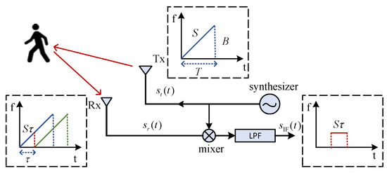
Figure 1.
FMCW radar block diagram.
The transmitted signal can be expressed as
where denotes the carrier frequency, represents the initial phase, and A is the amplitude. The chirp frequency changes uniformly throughout a single period T with a change rate S and a bandwidth B.
After the signal is reflected, the receiver mixes the received signal with and uses a low-pass filter to acquire an intermediate frequency (IF) signal, which is given by
where , , and denote the IF, the amplitude, and the phase of the IF signal, respectively. By preprocessing the IF signal, the point cloud information can be obtained (Section 3).
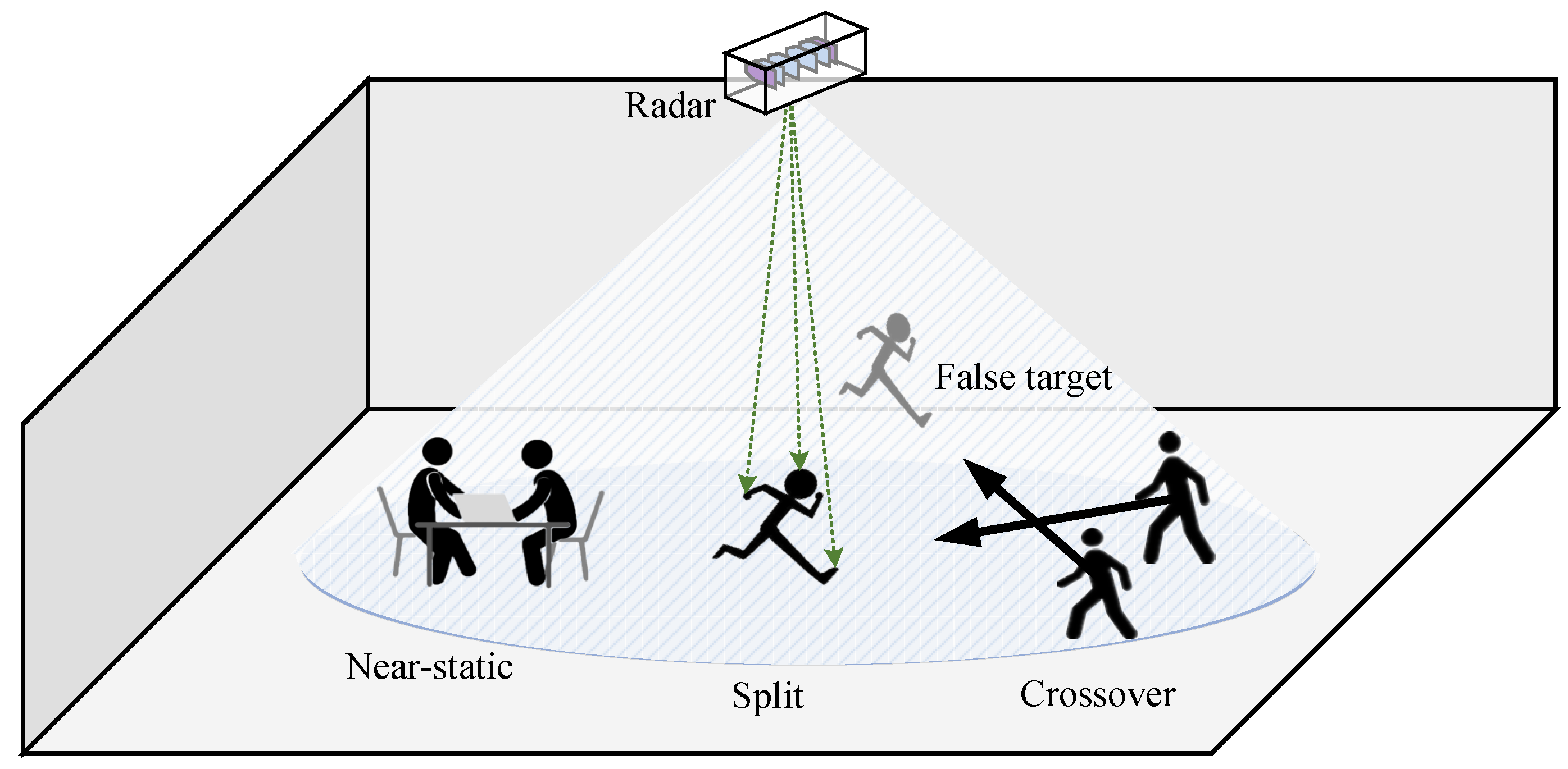
These measurement points will be entered into the tracking module (Section 4), which aims to track each indoor target continuously and robustly with as few false targets as possible. The number of people tracked varies from one to ten, and in order to imitate real-life events, the states of these persons usually change. Some states and issues create considerable obstacles to the continuity and resilience of the tracking system. These complex problems are shown in Figure 2.
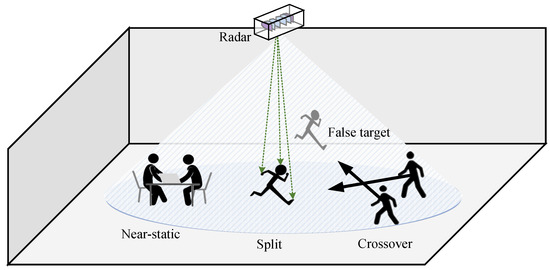
Figure 2.
The challenges of indoor tracking.
They are characterized as follows:
- Track split:Human targets perform actions such as arm swinging, which extend the measurements significantly. Some measurements from a single target are considered to belong to a new target.
- False target:Targets resulting from measurements that are not human targets are referred to as false targets. Measurement sources can be clutter, multi-path effects, and direct current component.
- Targets’ crossover:Several human targets are simultaneously approaching. This is characterized by the merging of point clouds, which results in association mistakes or the loss of targets.
- Near-static target:The human target hardly moves while seated or lying. It is characterized by the fact that there is less information in the target point cloud and that there is frequently no measurement of the target in multiple frames, leading to the loss of the target.
The traditional PTT method is less effective in complex multi-target scenarios because it ignores the expansion characteristics, neglects the overall track information, does not consider the multi-path effect, and is highly dependent on the clustering effect. In order to cope with the complex indoor situation in daily life, a novel tracking method is proposed in this paper to solve the above tracking problems.
3. mmWave Radar Signal Preprocessing
The IF signal described in Section 2 must be preprocessed to obtain the necessary target parameters before tracking. The chain of signal preprocessing implements the range-Doppler (RD) information acquisition, static clutter removal, measurements’ detection, signal-to-noise ratio (SNR) estimation, and elevation–azimuth (EA) information acquisition and, finally outputs the point cloud including the range, Doppler, azimuth, elevation, and SNR. The flowchart of signal preprocessing is shown in Figure 3.

Figure 3.
Diagram of the proposed signal preprocessing workflow.
3.1. RD Information Acquisition
Specifically, the IF signal can be stated as follows when the target is located at a distance of d meters from the radar:
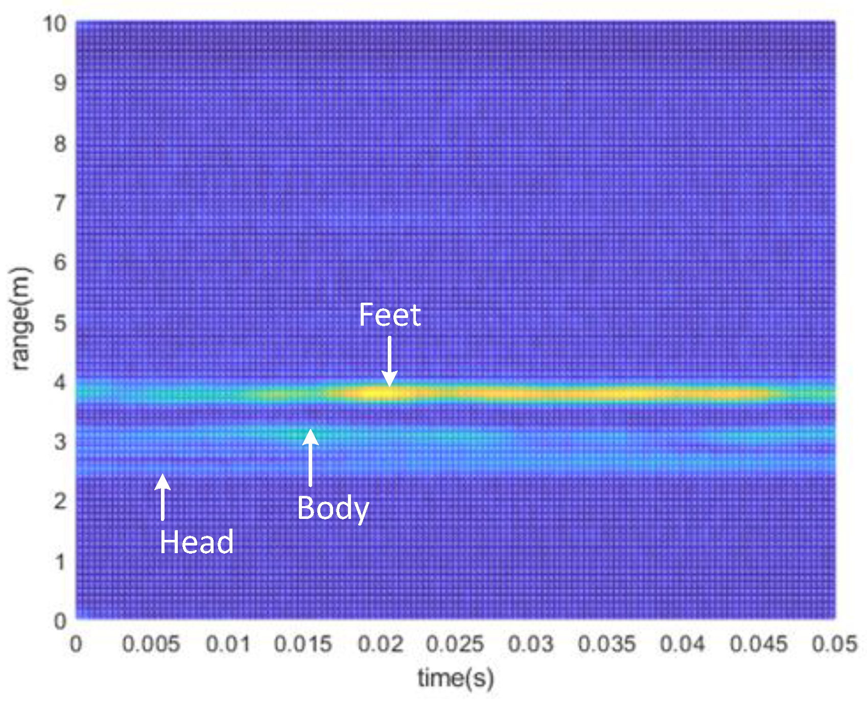
where , , c is the speed of light, and represents the wavelength. It is demonstrated that objects at different distances can generate IF signals with specific frequencies, which enables the Fourier transform [23] in the fast time dimension to separate various instantaneous frequency values to obtain the range information of multiple objects and create a range map. It is worth noting that the range profile can show significant scalability with numerous isolated peaks, even in the single-target scenarios shown in Figure 4, due to the height of the human body.

Figure 4.
Range profile when there is only one target in the field.
Additionally, the signal phase is susceptible to minor object displacements. Considering that successive chirps separated by have a phase difference , the Doppler can be calculated by
3.2. Static Clutter Filtering
There is no interest in stationary items since we focused on locating moving targets. RD maps contain noise at zero frequency, which can severely affect the detection and tracking of moving objects. These clutter signals are created mainly by the surroundings indoors, including floors, walls, and tables and other furniture, which have velocities near zero. Therefore, a moving target indication (MTI) method [24] is used to detect and suppress static clutter from the Doppler dimension.
First, by averaging all chirps in a single frame, the reference receiving chirp can be calculated as
where represents the r-th fast-time DFT point in the d-th slow time and N is the number of slow-time DFT points. For moving targets, the signal phase changes as the target moves; thus, the phase of each chirp is different, resulting in phase cancellation, which reduces the amplitude of the reference chirp. After subtracting the reference receiving chirp from all chirps, the amplitude of the moving target rarely changes, whereas the amplitude of the stationary target is decreased.
Compared with the commonly used two-pulse cancellation [25], the background noise of this method is cleaner and more suitable for multi-target detection scenarios with multiple peaks.
3.3. Measurements Detection and SNR Estimation
After static clutter filtering, the RD map shows numerous distinct peaks. The ordered statistics constant false alarm rate (OS-CFAR) [26] detector is a method for estimating interference level thresholds adaptively and ensuring a constant false alarm probability. The clutter properties of the current unit to be detected (CUT) can be approximated using data from adjacent units.
First, the N reference cells are sorted from smallest to biggest, and the k-th sample is selected as the background clutter power level . Then, cells exceeding the adaptive threshold are referred to as detected measurement points, where is a constant value. Next, the SNR for a CUT of power is estimated to be . This method is more sensitive to continuous multi-peak scenarios and more appropriate for multi-object detection than the widely applied cell averaging constant false alarm rate (CA-CFAR) detector [27].
3.4. EA Information Acquisition
Conventional angle of arrival (AOA) estimate methods [25] are constrained by the limits of physical angle resolution and cannot precisely measure angles. Since DFT in the antenna dimension is far from meeting the requirements, the minimum variance distortionless response (MVDR) algorithm [24] is required to obtain the target angle, which is a super-resolution beamforming technique.
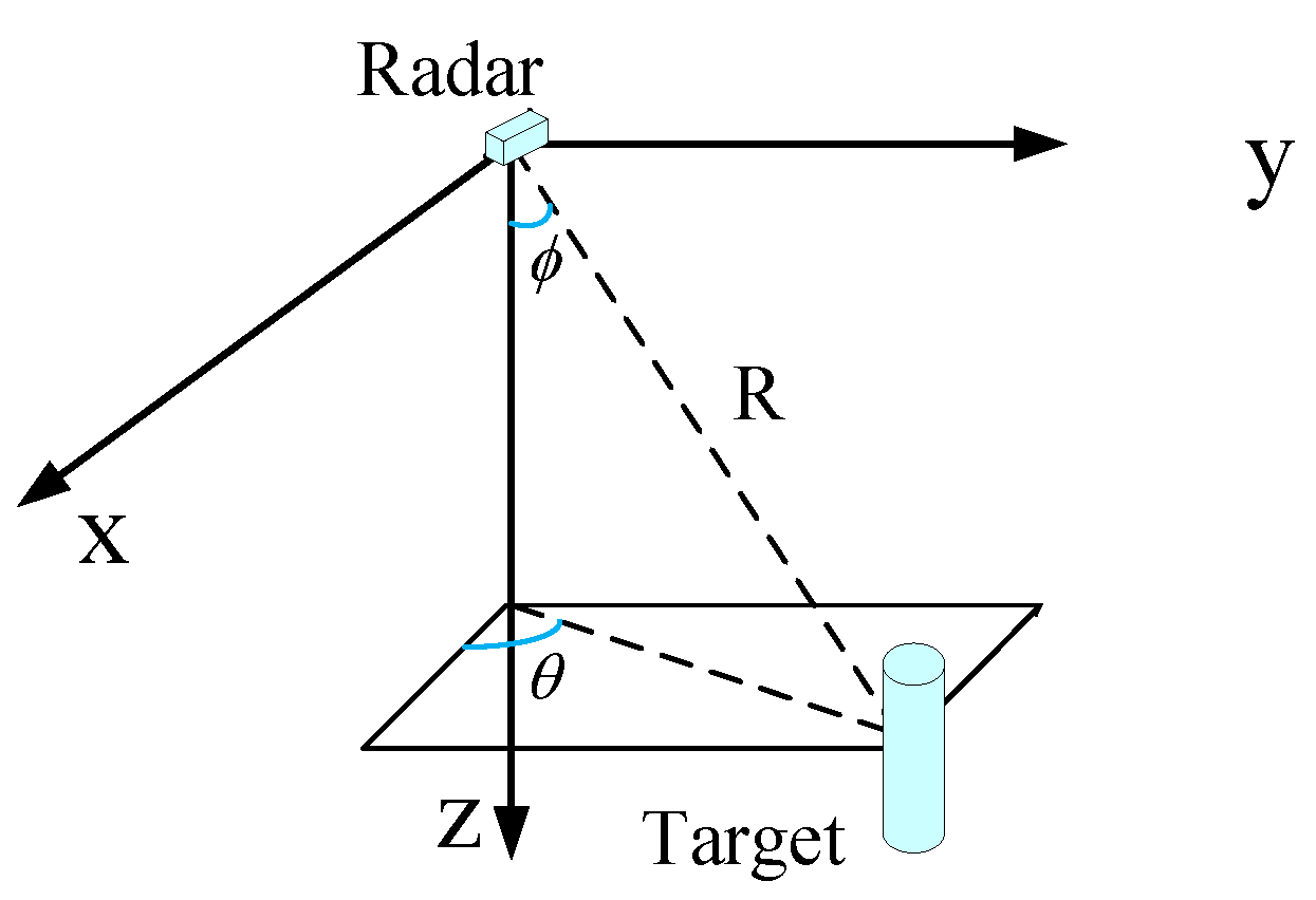
First, the experimental scene can be modeled as shown in Figure 5, where a Cartesian coordinate is formed with the radar as the origin of the coordinate, indicates the elevation, whereas represents the azimuth.
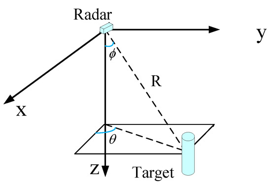
Figure 5.
Cartesian coordinate system diagram of the experimental scene.
Assume that and are horizontal and vertical equivalent array element intervals, respectively, and the phase shift of the incident wave to the array element relative to the reference signal point is
Its power spectrum can be expressed as:
where , , denotes the steering vector, ⊗ is the Kronecker product, and represents the receiving signal.
The EA profile can be generated by analyzing all elevation and azimuth angles in the power spectral space, followed by CA-CFAR and connected domain analysis to create single or multiple connected domains. A reference point is chosen in each connected domain to serve as the angle information for the reflected point. When detection points are obtained from the RD profile and detection points are obtained from the EA profile in the frame k, a total of reflection points are obtained in a single frame.
3.5. Point Cloud Generation
Because the range and angle information of each measurement point has been obtained, the position information can be obtained through three-dimensional mapping:
Assume that the i-th reflection point vector contains information about its location in a polar coordinate system and can be expressed as , and the elements within the vector are the range, Doppler, azimuth, elevation, and SNR. The final point cloud set will be entered into the tracking module.
4. The Proposed Tracking Method
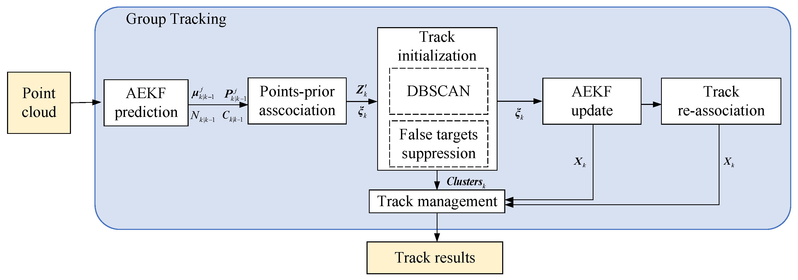
The signal preprocessing described in Section 3 generates a series of point cloud collections at instant k. For each frame of the constantly transmitted point cloud, our method carries out the following tracking processes depicted in Figure 6.
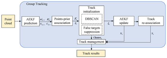
Figure 6.
Block diagram of the proposed tracing process.
The proposed method performs the following process sequentially:
- Prediction:For the prediction of multi-dimensional information on targets, an AEKF method suited for extended targets is employed. The number of reflected points corresponding to a single human target is estimated using alpha filtering, and the extension information is characterized by the multivariate Gaussian distribution covariance. In this step, we can obtain prior information, including the position, velocity, covariance, number of points, and extension.
- Points-to-prior association:Given the prior expectations and multiple reflection points obtained, the number of data association assumptions is extremely high, and GNN is a practical association estimation approach. It prunes posterior density estimates with the exception of the best estimate. Since the processing is not point target tracking, the classic GNN “one-to-one” distribution strategy cannot deal with human target point clouds. Therefore, a “many-to-one” point cloud association technique is paired with gating to associate all reflection points belonging to the same human target with the relevant prior expectation. When the quality of the point cloud on the field is insufficient, this approach can nonetheless correlate and preserve the target track across numerous frames.
- Track initialization:A density-based spatial clustering of applications with noise (DBSCAN) with false target suppression is utilized to acquire several emerging targets throughout the tracking procedure, which is exclusively employed for unassigned point clouds. Simultaneously, the method estimates all present subjects during the first frame of the complete tracking process. In addition, we improved the initialization scheme to make it more suitable for mmWave indoor applications in terms of target split and false targets. According to the number of people, the clustering parameters can vary adaptively to fit the changing quality of the point cloud for each individual.
- Update:The reference centroid of the related group is determined using a weighting approach based on the SNR of various reflection points. According to the number estimation and extension estimation produced through filtering, the AEKF is used to estimate the posterior information by adjusting the measurement noise estimation adaptively to ensure updating the extended target accurately. The mean of the posterior multivariate Gaussian distribution is then used as the target state estimation. Additionally, a person counting process is performed during this phase.
- Track re-association:To address the issue of track break, a track re-association approach is presented for quasi-static targets and track fracture, which may be brought on by occlusion or crossover. To be specific, people can interact more frequently as the number of people grows. As the target velocity drops, the target information may be filtered out as static clutter. This may cause several fractures in the track, as well as the loss of point clouds of specific targets in subsequent multiple frames. With this method, the attribution of the new trajectory is determined by comparing how similar the old and new tracks are.
- Track management:Track management includes track status such as temporary, active, reserved, leaving, and released tracks. This process transfers the status of trails between multiple pre-set states through specific judgment standards, ensuring the initialization of new tracks, the update of continuous tracks, the retention of unassociated tracks, and the release of free and leaving tracks, which can be seen in Figure 7.
 Figure 7. The changes in target and track states throughout the proposed group tracking model.
4.1. Alpha-Extended Kalman Filter
In order to not only filter the target position, Doppler, and covariance, but also continually evaluate the number of reflection points and extension information, we propose an AEKF in the prediction and updating process. The C-K equation, which is computationally intensive, is used in Bayesian filtering to determine the prior information [28]. To lower the computing expenses, the following assumptions were adopted: (a) prior density follows a Gaussian distribution with a mean of and a covariance of ; (b) the detection probability is constant; (c) measurement likelihood follows a Gaussian distribution with a mean of and a covariance of ; (d) clutter intensity . The specific calculation process of the above parameters will be given later in this subsection.
Suppose that there are active targets in the previous frame and the posterior estimate of the j-th target state is , including the target position ( and ) and the target velocity ( and ). The target extension is estimated to be , containing the number of reflection points and extension . The target posterior state covariance matrix is . In addition, we define the m-th reflection point taken from the sparse point cloud generation module in this frame to be with .
For the target moving model, a constant-velocity motion (CV) model [29] was selected. However, even if the CV model is employed, the target is not required to move at a constant speed. The velocity change in one frame can be fully characterized by process noise since the acceleration of the human target is low. The target state transition matrix is defined as follows:
which describes the expected state change between two adjacent frames, is the time of one frame, and is the identity matrix.
The prior information of the target state and covariance matrix for target j is calculated as
where , and represents the covariance matrix of process noise, which follows a Gaussian distribution with zero mean. Moreover, in the prediction step, assume that the prior information of the number of points and expansion remains the same, i.e., , .
The collected point cloud is in Cartesian coordinates, and the target state must be mapped from the Cartesian space to the polar coordinate space using an observation equation with a nonlinear function. The Jacobian matrix [30] is used to linearize the nonlinear function by Taylor expanding and retaining the first-order component of the expansion terms to obtain the observation matrix .
During the update phase, a series of reflection points associated with the target is gathered. The sequence numbers of reflection points related to the j-th prior expectation are defined by with a length of . The association process will be elaborated upon in Section 4.2.
First, we updated the group expansion and the estimated amount of points. The extension is defined as the covariance matrix of the SNR-weighted mixture Gaussian distribution consisting of all correlation points, which can be obtained using the EM algorithm [31]:
where represents the mean value of all associated points.
The values of and were set as constants, and the number of the target reflection points was updated to
The extension is calculated as
Meanwhile, the target posterior state is expressed as
The target covariance is
In the above equations, the Kalman gain is written as , and stands for the reference point of the group, which is the SNR-weighted mean of related points.
Moreover, conventional PTT often assigns a constant value for that is of interest. By considering the time-varying character of ETT, is defined as an equation involving the number of expansion and reflection points:
The first part of (17) represents the observed noise covariance of the single reflection point, where is the difference between the maximum and minimum values of each dimension in the associated sequence; the second part of (17) is the estimation of the expansion, whose physical significance is that, as the expansion becomes larger, the uncertainty of the measurement increases, which leads directly to the target posterior covariance becoming large. Furthermore, a constraint is placed on the value of to avoid situations where convergence is impossible. In practice, it should be less than the approximate length of the open arms of the human body and larger than the width of the human shoulders.
The complete process of the algorithm is demonstrated in Algorithm 1.
| Algorithm 1: AEKF. |
|
Compared to the standard extended Kalman method, the proposed method benefits from considering the “many-to-one” association in the case of ETT, which ensures that the posterior density covariance can accurately model the uncertainty and enhances the accuracy of tracking associations.
4.2. Points-to-Prior Association
Target association is a crucial step that substantially decreases the number of posterior mixing density components. In other words, only the major components of the Gaussian mixture density are maintained, while the minor parts are eliminated. It can significantly reduce the algorithm’s complexity while maintaining its efficacy. In PTT-like association processes, the Hungarian algorithm [32], Murty algorithm [33], and Gibbs sampling method [34] are frequently employed to determine single or many optimum allocation strategies. They are characterized by their “one-to-one” relationship, which is supplemented by a clustering technique before tracking in each frame to accomplish a priori cluster matching. This approach relies primarily on clustering, which might result in many association failures as the population grows and the quality of the point cloud deteriorates.
The non-normalized weight of the posterior mixture-density component resulting from the j-th prior expectation associated with the reflection point is
Under the assumption that the detection probability and clutter intensity are constants, we have
where , , and the calculation processes was described in detail in Section 4.1.
The entire general pseudocode to the algorithm is shown in Algorithm 2. After the procedure, a series of correlation sequences are obtained. In contrast to the standard PTT-like approach, we associated and matched each reflection point that satisfies the gating requirements to choose the best-matching track, so the number of reflection points associated with each track might be zero or larger than one. The gating parameter G changes in each frame based on the expected number of people on the field. Furthermore, is the association result, where stands for that for the c-th measurement whose optimal pairing is the j-th prior; means that there is no matching target for this reflection point. Finally, we obtain the associated sequence for each subject:
When it is not equal to 0, the sequence length is , which represents the number of reflected points matched by the track j, and is the index vector of these points.
| Algorithm 2: Group association. |
|
4.3. Track Initialization
For points that , the probability of a new target entering the field of view is considered. In our method, clustering is used to determine the possible new targets, while a false target removal method is applied to distinguish unreal targets within them.
DBSCAN can divide sufficiently dense areas into clusters and form arbitrary clusters in a noisy spatial database, where clusters are defined as the greatest group of densely linked points. This has benefits over k-means of not requiring the number of clusters to be specified in advance, not initializing the cluster center, and not being sensitive to noise. Thus, in crowded indoor situations, DBSCAN is better suited for human target initialization than k-means. Traditional DBSCAN requires just the parameters and , which describe the neighborhood radius and the minimum number of points, to classify and cluster a set of points.
However, on the one hand, there are cases of target splitting in mmWave tracking situations due to target expansion or inadequate angular resolution, which is shown in Figure 8a. A single human target may generate two distinct high-density clusters in the X-Y plane. Increasing the value of can mitigate this problem, but it will result in a single group when numerous new targets approach, which is shown in Figure 8b. On the other hand, multipath effects may generate ghost targets. These fake targets are related to the actual target movement for numerous frames in succession, as shown in Figure 9, finally generating a ghost trace.
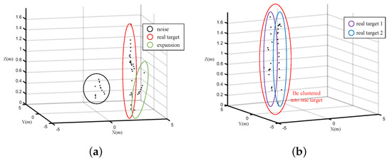
Figure 8.
The contrast between the point cloud formed by target splitting and the one created from approaching targets. (a) Single target splitting. (b) Two close targets.
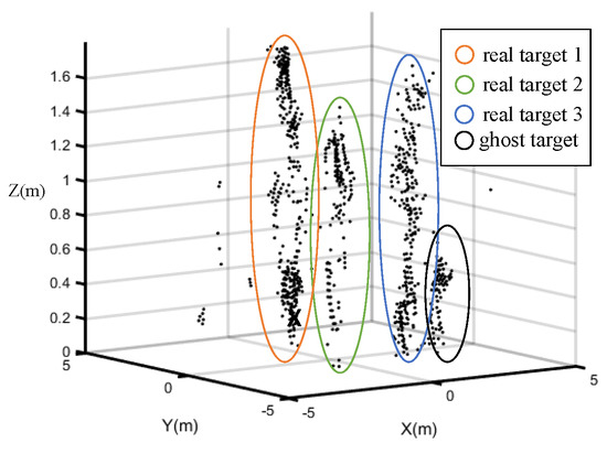
Figure 9.
Three−target scenario where Target 3 produces ghost measurements.
To address these two issues, we examined a vast quantity of measured data and investigated reducing the appearance of false targets from three perspectives: cluster location, cluster centroid height, and cluster SNR.
Suppose that the unassociated points can be written as , whose length is equal to . They are entered into the new target initialization module, and DBSCAN and false target removal algorithm are executed. The methods are shown in Algorithm 3. After the algorithm has completed, the track management module initializes temporary tracks for the new targets since are considered new human targets in this frame.
| Algorithm 3: DBSCAN-based false target suppression. |
|
4.4. Track Re-Association and Missing Track Estimation
Given a track variable , where represents the short track start time, denotes the short track stop time, and is the posterior estimate of successive target locations, the possibility of track matching was considered. Duplicate tracks reserved by track management were not considered, as these reserved tracks will change the natural features of the trajectory. Moreover, considering the complexity of human target movement, the value of is not the start time of the complete global track, but rather the artificially set start time of the local short track. The analysis was restricted to the latest 40 distinct track states, from which we obtained the of each .
At the moment k, a sequence of trajectories is produced and entered into the re-association module. We assumed that the current target state is related to the target states of the historical M frames. Then, the target state model can be represented by the linear regression relationship:
where M is also referred to as the regression model order, which determines the state model complexity, and is the weight of the order i. The re-association method is based on this premise of the regression model. The procedure is displayed in Figure 10.

Figure 10.
The process of track re-association.
The motion state (static or moving) of tracks needs to be identified first. The state variation of each short track is calculated, and we labeled it as stationary if the variance was less than the threshold; otherwise, we identified it as a moving track. Next, the moving and stationary tracks will be separately re-assigned.
4.4.1. Track Re-Association for Moving Target
For tracks and identified as moving targets with non-overlapping time, the time, slope, and state differences (, , and ) are calculated. If these three values exceed the thresholds, they are marked as possible homologous track pairings. After obtaining a sequence of potential homology track pairs, the completed track variable is denoted by , and the trajectory is , where stands for the estimated missing trajectories. The n-order Hankel matrix of can be obtained as follows:
where n is produced under the condition that the Hankel matrix arrangement becomes a square matrix; otherwise, the matrix can be interpolated.
As the minimized regression model can be converted to reduce the rank of the Hankel matrix [35], the lost track of the chosen track pair can be calculated by . This issue can be translated into a semi-positive definite problem as follows:
where X and Z are free variables and is the trace of the matrix.
Then, for these completed tracks, define the correlation probability of the short track variables and :
The rank of the matrix is solved using SVD decomposition, and the cost matrix is derived according to the correlation probability, with the likelihood that the track is associated with itself set to infinity. Finally, we used the Hungarian algorithm [32] to calculate the following optimal allocation problem:
where represents the allocation matrix and p is the number of short tracks participating in the allocation. Once tracks and are successfully re-associated, will be deleted and will be set in the track management module.
4.4.2. Track Re-Association for Near-Static Target
Short tracks and , marked as stationary targets with non-overlapping time, are identified as possible homologous pairs when their mean states and time difference are both below the thresholds. Indeed, practically stationary tracks frequently break several times. Thus, we decreased the correlation cost by the number of track re-associations . Assume the cost of inactive target association as the Euclidean distance divided by the number of re-associations, which can be expressed as
As the time of the re-associations of a stationary target grows, the target is more likely to be an actual, stationary target instead of clutter and, hence, has a lower correlation cost. The optimum allocation problem is then solved using the Hungarian method to produce the association result. In addition, because it is of little necessity to estimate the lost track of a stationary target, linear interpolation is used to calculate the estimated track and trajectory variable . After assignment, in the track management module, the track will be deleted, and then, we set and .
4.5. Track Management
To guarantee that the tracking method can retain a high degree of resilience in the case of false tracks, target entrance, exit, etc., the track management module separates the tracking status into five stages based on a combined evaluation of multi-frame association and re-association information: temporary, active, reserved, leaving, and released tracks.
When a new cluster is formed, the new target track is initialized as temporary until it has been successfully associated M times in the previous N frames. When an active trajectory fails to be associated continuously in the last K frames, its status is changed to be reserved to ensure that the two tracks can be re-associated after beginning a new track of the same source. Once it is determined that the track cannot be re-associated in the previous frames, it will be released. The state of the trajectory determines the values of K and , which is evaluated in Section 4.4. To be specific, these two thresholds have lower values for moving targets and larger values for stationary targets. Moreover, the values are lowest for targets at the field of view bounds, which are referred to as leaving tracks.
5. Experimental Results
In this section, the effectiveness of our strategy was analyzed from many distinct perspectives. The TI IWR6843-ODS [36] was used in the experiments, which has three transmitting and four receiving channels, operating on time domain multiplexing (TDM) from 60 GHz to 64 GHz. Figure 11a depicts the radar and virtual equivalent antenna array. Figure 11b illustrates the experimental area selected, with the radar installed on a bracket approximately high in the center of the area and the radar points directly downward. Simultaneously, we placed a camera facing the trial site to obtain the real target trajectory and the identifying information. Figure 11c is a video screenshot of the seven-person free-motion-counting experiment, which shows the room setup in which we conducted the experiment.

Figure 11.
Overview of the experimental setup. (a) The radar and the virtual equivalent antenna array. (b) Schematic diagram of the experimental scene. (c) The experimental scene of seven people in the field.
Instead of utilizing integrated DSP to acquire point cloud information, the original radar echo is transmitted straight from the sensor to the computer. On the computer side, the modules for point cloud generation and multi-target tracking are performed to continually capture the trajectory and ID. Table 1 outlines the used radar parameters.

Table 1.
Radar parameters.
In the experiments, unless otherwise stated in the subsection, human behavior was not constrained, which means that the targets walked as they do daily and were allowed to approach each other. The speed of the targets was the speed at which humans usually walk.
5.1. Evaluation of Tracking Accuracy
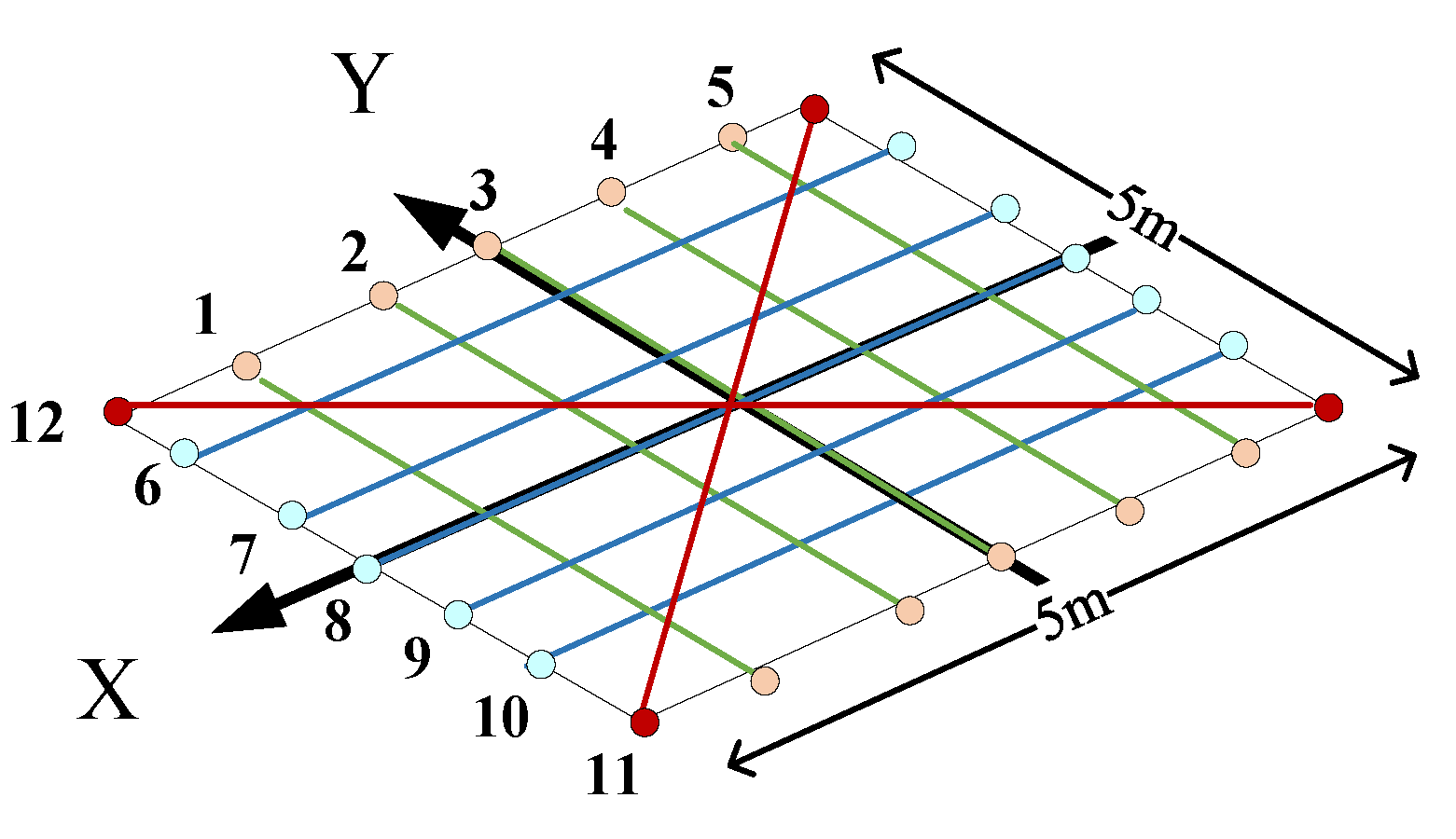
In order to verify the accuracy, the error of the tracking results needed to be quantified. Only the single-target scenario was considered here, and the target walked in a straight line according to the pre-set trajectory, as shown in Figure 12, wherein the size of the experimental area was . The distance between each adjacent start (end) point was 1 m. The blue and green lines represent the trajectory parallel to the X and Y axes, respectively, and the red line represents the trajectory located diagonally. The target walked back and forth on the path. For each route, 2 sets of data for two targets were collected, and 24 sets of data were obtained.
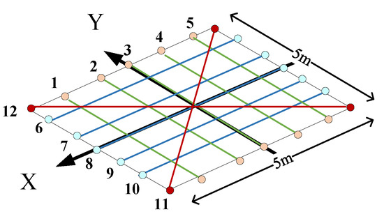
Figure 12.
The preset target trajectories.
Assuming that the pre-set path can be expressed as and the estimated position of target at the moment k is , then the position error can be written as
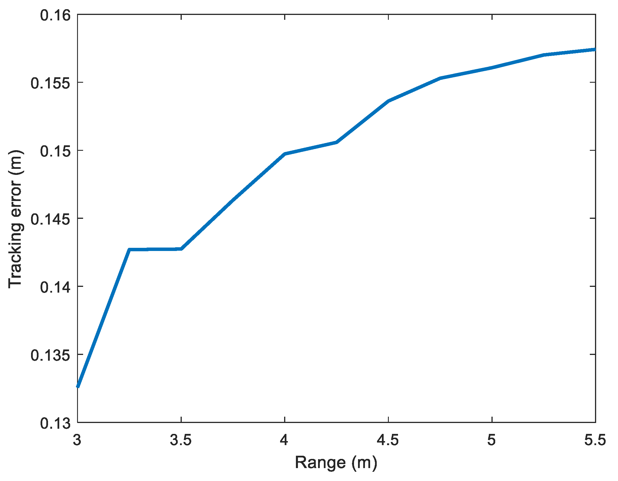
where A, B, and C are all constant. The tracking error for each set of data is defined as , where K represents the total number of frames. Depending on the distance at which the target is located, the tracking error of different distances can be calculated, as demonstrated in Figure 13.

Figure 13.
Evaluation of the tracking error.
It can be seen that, as the distance between the target and the radar increased, the tracking error also increased. The reason why the distance started at 3 m was that the radar was 3 m high, and the maximum distance was constrained by the maximum angle that the radar can detect. In addition, the average tracking error for the 24 sets of data was 0.15 m.
5.2. Evaluation of False Track Removal
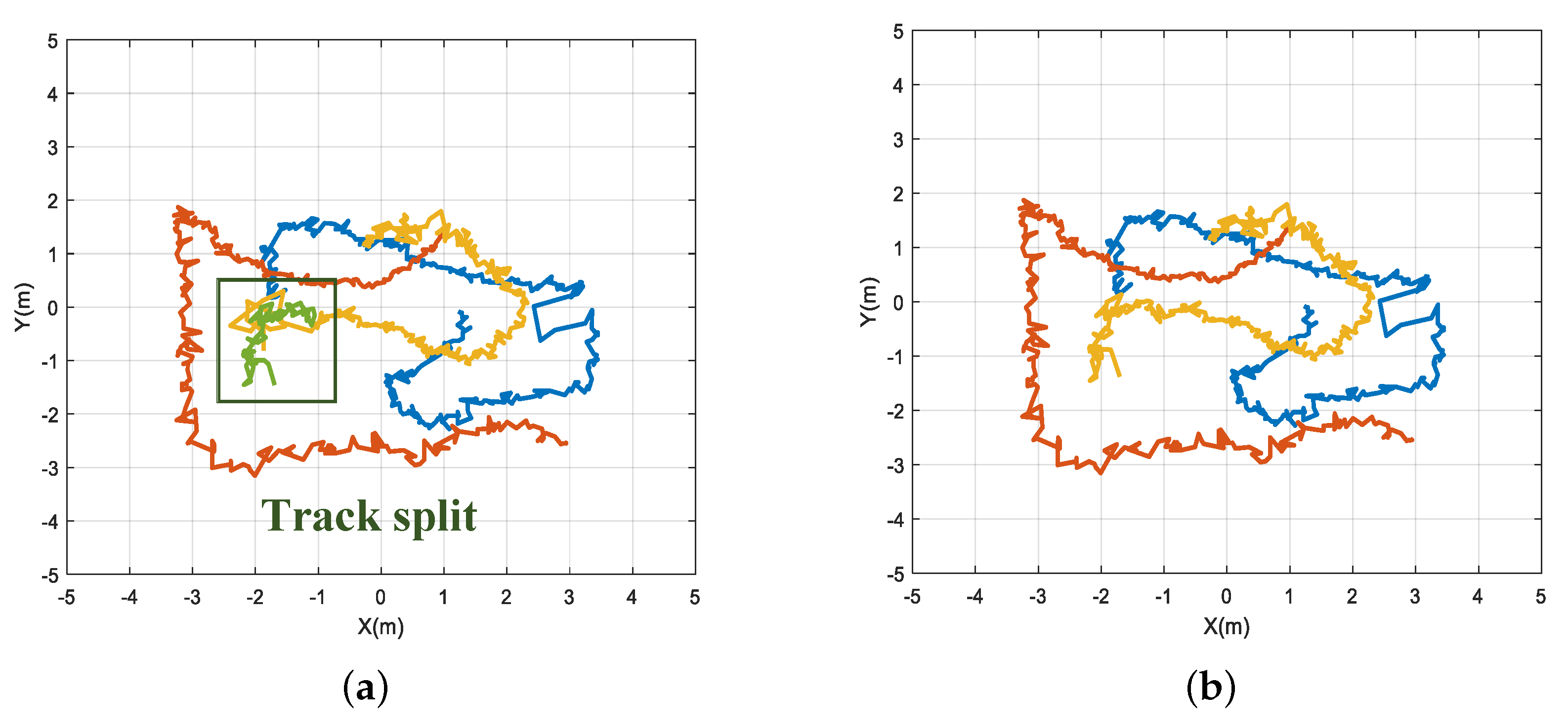
To evaluate the method against the target splitting problem, we developed the following experimental content: the targets walked freely in the scene while simultaneously shaking their bodies to enhance the degree of target expansion. Owing to the constraints of the DBSCAN algorithm, the conventional approach generates false targets, which are often retained for a long time due to the “points-to-target” association scheme of group tracking. In Figure 14 and Figure 15, the false target produced by extreme expansion and the influence of ID switches on continuous monitoring were successfully removed.

Figure 14.
The tracking results at Frame 273 of free movement situation of three people swinging their bodies. (a) Track 2 splits, producing False Track 5 in front. (b) After using our method, Track 5 is determined to be caused by target extension.
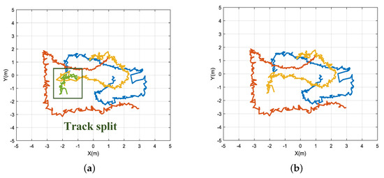
Figure 15.
The accumulated tracking results of free movement situation of three people swinging their bodies. (a) The accumulated track result plot before applying our method. (b) The accumulated track result plot after applying our method.
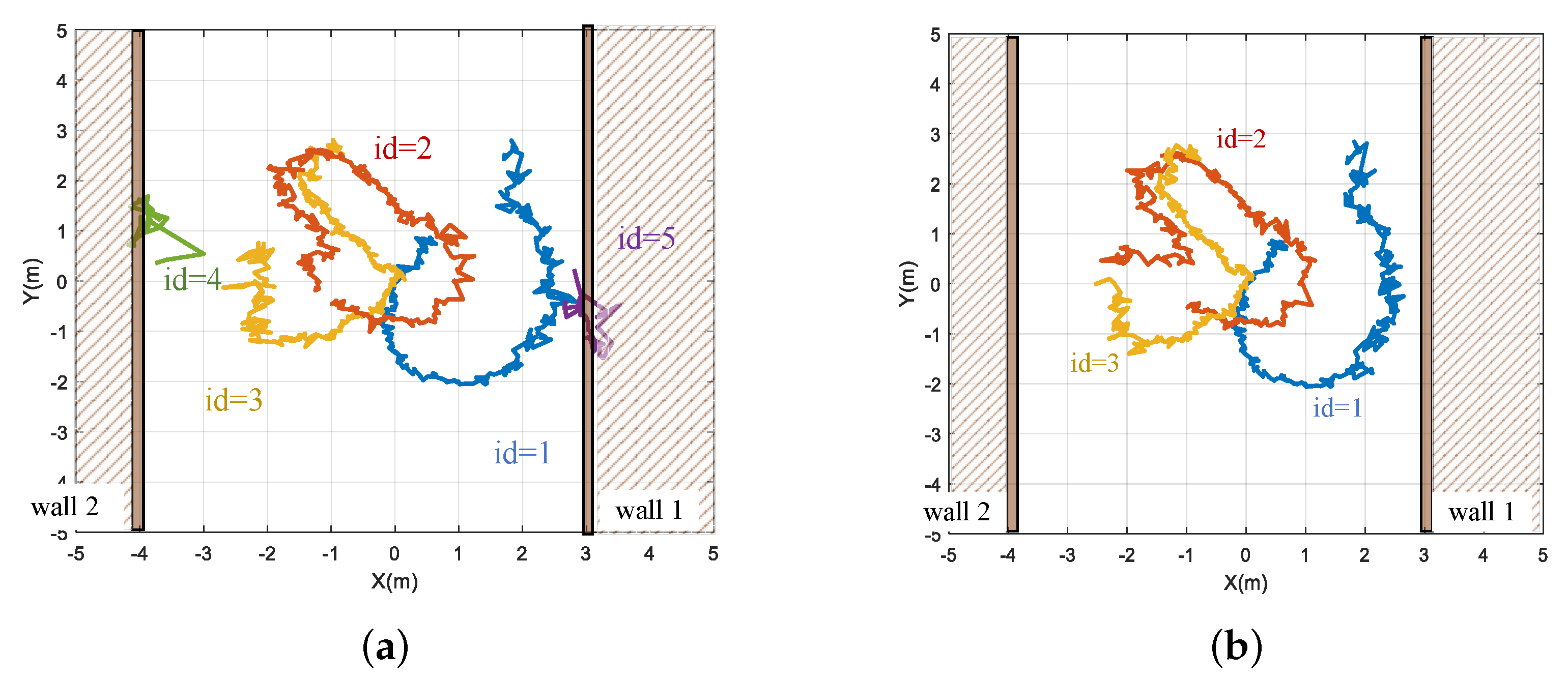
Furthermore, the multi-path effect may generate false alerts when the target is adjacent to a wall. Several targets were instructed to walk freely and were permitted to approach the wall to generate visible ghosts in this subsection. Figure 16a,b show the results. By conducting false target suppression after DBSCAN, the ghost tracks were suppressed, and the temporary path of the real target was initialized sooner, as the false target was no longer associated with the reflection point of the real target.
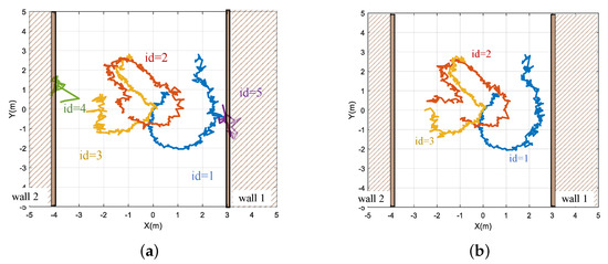
Figure 16.
Comparison of using and not using the proposed ghost target suppression and AEKF method. (a) Ghost Tracks 4 and 5 appear, and the initialization of Tracks 1 and 3 is affected by Ghost Track 4. (b) After using our method, Tracks 4 and 5 are determined to be caused by the multi-path effect.
5.3. Evaluation of Expansion Estimation
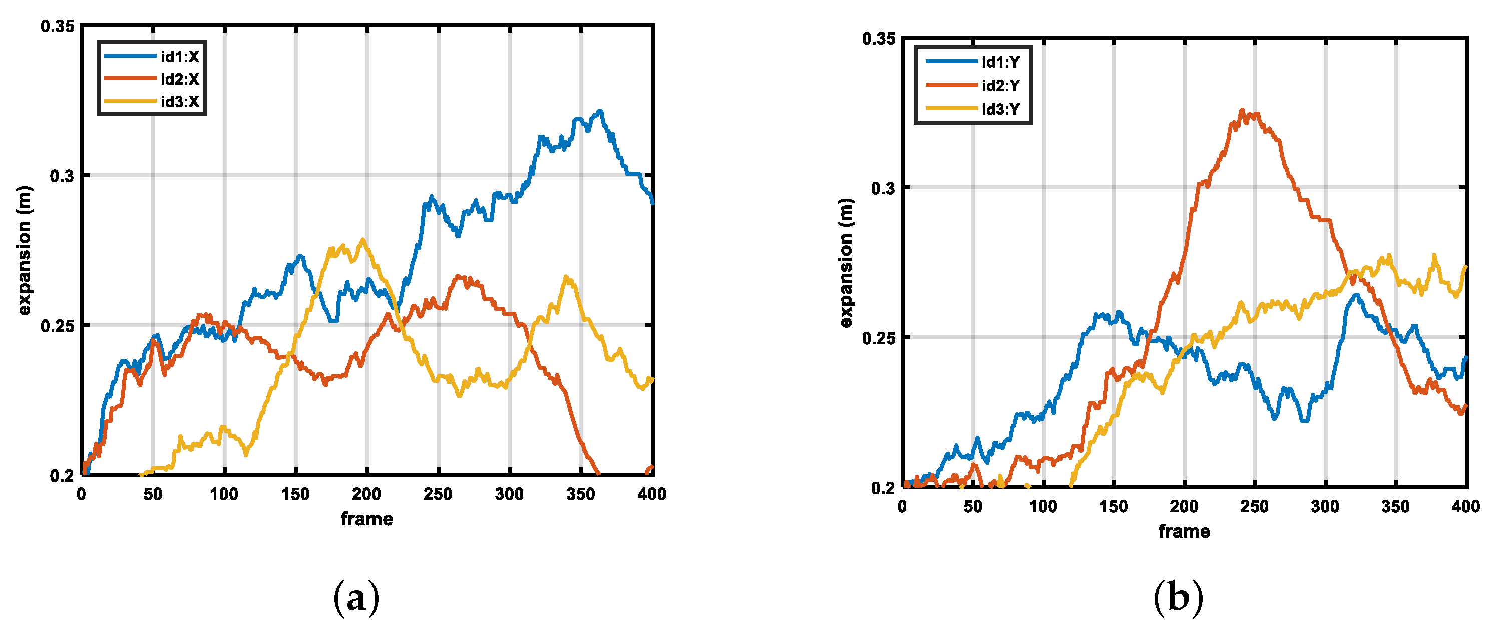
Due to the application of extension estimation in AEKF, Track 2 in Figure 16b approaches the wall without interference from ghost reflection points. We selected the x- and y-direction extensions to evaluate the estimated extension. The value that has been alpha-filtered is presented in Figure 17. It can be seen that the degree of expansion impacted the estimate of the observed noise to achieve maximum association with all of the target reflection points. From the track results, one can see that when the expansion of one direction rose, the degree of track oscillation in that direction also increased.
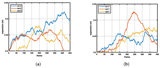
Figure 17.
The estimated degree of expansion. (a) The expansion of the targets in the x-direction. (b) The expansion of the targets in the y-direction.
5.4. Evaluation of Targets’ Crossover
In the crossover scenario, our approach displayed remarkable resilience. In the experiment setup, the number of persons present climbed from 2 to 6. For the circumstance where there were more than two persons on the field simultaneously, except for the two targets that intersected, the rest of the people moved freely in the trial area. Both intersecting targets were required to begin from the same side, approach at a predefined point, and then, go straight, make a sharp angle turn, make an obtuse angle turn, or return the same way, as demonstrated in Figure 18.

Figure 18.
The intersection cases of two intersecting people considered.
In the collected dataset, each case of crossover accounted for about a quarter of the dataset. Tracking accuracy is defined as the number of crossings correctly tracked divided by the total number of crossings. Table 2 illustrates the tracking accuracy, which shows that the proposed method achieved more than 90% tracking accuracy in crossover scenarios with six or fewer participants. Case 4 was the crossover case with the most tracking errors for the above four cases. The reason was that, when one of the targets turned back early, its associated reflection point may be misidentified as belonging to another target. The tracking results of the remaining three cases were similar.

Table 2.
The tracking accuracy of the targets crossover.
During the experiments, it was discovered that the velocity and the distance between the targets at the intersection mainly influenced the tracking accuracy. The association was prone to fail when the targets were close and moved quickly through the intersection, which might cause the target to vanish or move in the wrong direction. When the target vanished, our re-association strategy could recover the missing track. However, the tracking result will be affected if the tracking direction is incorrect.
5.5. Evaluation of Track Re-Association
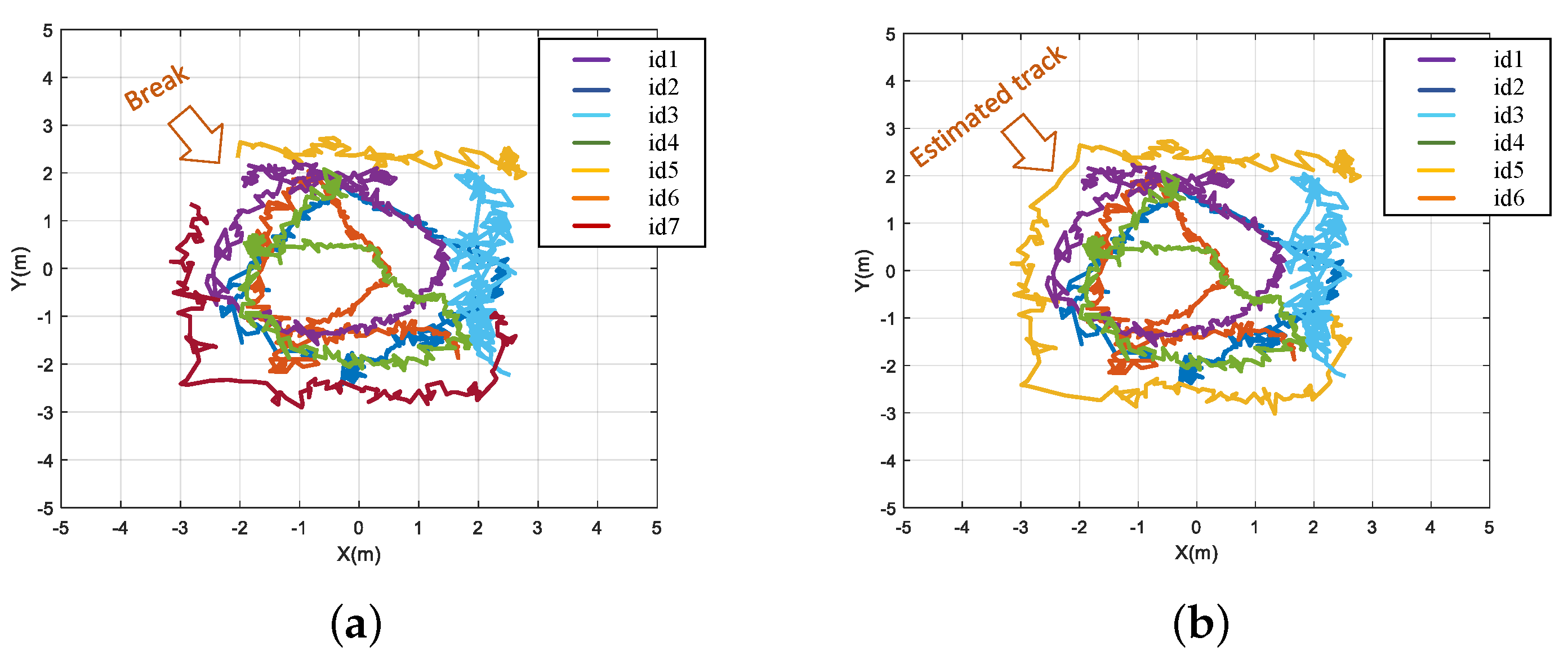
To demonstrate the consistency and efficacy of monitoring moving targets, we designed scenarios in which six targets moved freely inside the experimental area. When Target 5 walked to the edge of the field of view, the target positioning error was considerable and the SNR was low, causing the track to break, as shown in Figure 19. The track management module retained Track 5, and when Track 7 emerged, it was determined that they were homology track pairs and the optimal missing track was estimated.
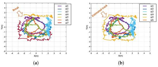
Figure 19.
Evaluation of moving track re−association. (a) Cumulative trajectory results without re−association scheme, and the short Tracks 5 and 7 belong to the same person. (b) Cumulative trajectory results after using the re−association and estimation scheme.
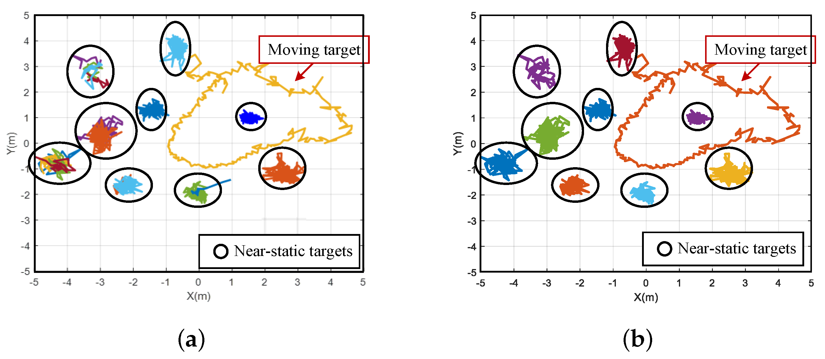
When a target was nearly stationary in the scene, its radial velocity was very low, and the information about it was lost during static clutter filtering, leading to an undesirable point cloud effect. The persistent missing association over multiple frames can cause numerous track breaks. In this experimental scenario, ten targets were on the field, nine of which slightly wiggled in place, and an individual wandered freely over the area. In Figure 20, each circle represents a true near-stationary target position and differently colored short tracks within one circle represent multiple breaks of the trajectory. The proposed method can effectively suppress the fracture of stationary targets from the dimension of the track. Due to angle inaccuracy and target limb swing, it was evident that the near-static target still expanded significantly. In addition, the walking person shuttled between them, and due to the continuous estimation of expansion, the trajectory was not affected obviously.

Figure 20.
Evaluation of near−static track re−association. (a) Cumulative trajectory results without re−association scheme. (b) Cumulative trajectory results after using the re−association scheme.
5.6. Analysis of the People Counting and ID Switch Result
In this subsection, the accuracy of the target counting is evaluated. Unrestricted motion datasets were collected with less than eleven individuals. In particular, six sets of data for each distinct number of persons present were gathered, for a total of sixty sets of data. The estimated tracks from the re-association module were counted as an actual target, generating tracks in the counting results. Target counting accuracy A is defined as
the proportion of the estimation error that is less than or equal to 1 is defined as
where represents the number of frames for which the counting result is T, which is the correct number of people, and N is the total number of frames.
In contrast, the TI group tracking method [37] was also used to process data in addition to the proposed method. In both algorithms, the preprocessing method and the values of the same parameters were set to be precisely the same.
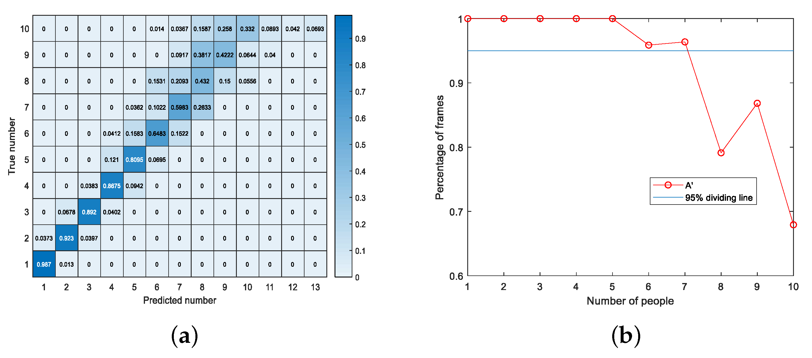
The results of the target counting are demonstrated in Figure 21. The value of A decreased monotonically as the targets increased and dropped significantly when the targets reached eight, which was due to the target body collisions and hesitations. Nevertheless, as shown in Figure 22b, remained above 95%, proving the high robustness of target counting.
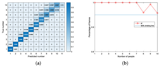
Figure 21.
Target counting accuracy analysis of the proposed method. (a) Confusion matrix for counting accuracy A of our work. (b) Line chart for of our work versus the number of people.
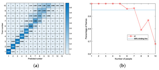
Figure 22.
Target counting accuracy analysis of the TI method. (a) Confusion matrix for counting accuracy A of the TI method. (b) Line chart for of the TI method versus the number of people.
As seen from Figure 22a, our tracking method tended to underestimate the number of targets because when the number of people reached more than eight, the target point cloud information became incomplete. The real target may be challenging to initialize or considered as a false target. Even if it becomes a temporary track, it may still need to be successfully transformed into an active track. In contrast, the counting accuracy of TI method is shown in Figure 22. The accuracy significantly reduced, especially when more than five people were simultaneously on the field. When the number of people reached ten, it can be seen that the counting error became more considerable.
Since the TI method is prone to false targets or breaks, “ID switch” was also added as an evaluation metric. It is defined as the maximum track ID minus the number of actual tracks, revealing the continuity and authenticity of tracked trails. For datasets of five or more people in this subsection, the average ID switch value for each dataset was calculated, as shown in the Table 3. The proposed method had a lower ID switch value, which means fewer false targets and fewer breaks.

Table 3.
The ID switch result.
6. Conclusions
In this paper, we proposed a novel group tracking method, including the signal preprocessing, AEKF, group association, new target initialization, false target suppression, track management, and track re-association methods in sequence. Several experiments were designed to verify the feasibility and effectiveness of the proposed approach. The results showed that the proposed method was significantly superior in continuity and counting accuracy to previous methods, especially in crowded indoor scenes. Specifically, it could guarantee the continuity of moving and static target trajectory, the suppression ability of false targets and splits, and the continuous estimation of target expansion. In the case of target crossing, the tracking accuracy rate can reach more than 90%. In addition, the counting accuracy rate reached more than 80% in the case of seven people or less and still achieved 58% in the case of ten people. In contrast, the TI group tracking method only reached 59% in the seven-person situation and decreased to 33% at ten. Our future work will consist of trying to use deep learning methods to achieve target identification during tracking. Furthermore, we will continue to focus on improving tracking accuracy in complex situations.
Author Contributions
Conceptualization, S.G. and M.J.; methodology, M.J.; software, M.J. and H.L.; validation, S.G., G.C. and Y.Y.; formal analysis, S.G.; investigation, M.J.; resources, M.J.; data curation, M.J.; writing—original draft preparation, M.J.; writing—review and editing, S.G. and H.L.; visualization, S.G.; supervision, G.C.; funding acquisition, G.C. All authors have read and agreed to the published version of the manuscript.
Funding
This research was funded in part by the National Natural Science Foundation of China under Grant 62001091, in part by the Municipal Government of Quzhou under Grant 2022D008 and Grant 2022D005, in part by the 111 Project under Grant B17008, and in part by the Guangdong Key Areas Research and Development Program under Project 2020B090905002.
Institutional Review Board Statement
Not applicable.
Informed Consent Statement
Informed consent was obtained from all subjects involved in the study.
Data Availability Statement
The data used to support the findings of this study can be freely accessed at https://github.com/meiqiuJiang/A-Robust-Target-Tracking-Method-for-Crowded-Indoor-Environments-Using-mmWave-Radar (accessed on 9 April 2023).
Conflicts of Interest
The authors declare no conflict of interest.
References
- Liu, H.; Wang, Y.; Zhou, A.; He, H.; Wang, W.; Wang, K.; Pan, P.; Lu, Y.; Liu, L.; Ma, H. Real-time arm gesture recognition in smart home scenarios via millimeter-wave sensing. Proc. ACM Interact. Mob. Wearable Ubiquitous Technol. 2020, 4, 1–28. [Google Scholar] [CrossRef]
- Wang, Z.; Yang, Z.; Dong, T. A review of wearable technologies for elderly care that can accurately track indoor position, recognize physical activities and monitor vital signs in real time. Sensors 2017, 17, 341. [Google Scholar] [CrossRef]
- Kolakowski, J.; Djaja-Josko, V.; Kolakowski, M.; Broczek, K. UWB/BLE tracking system for elderly people monitoring. Sensors 2020, 20, 1574. [Google Scholar] [CrossRef]
- Chen, J.; Zhang, Y.; Guo, S.; Cui, G.; Wu, P.; Jia, C.; Kong, L. Joint estimation of NLOS building layout and targets via sparsity-driven approach. IEEE Trans. Geosci. Remote Sens. 2022, 60, 1–13. [Google Scholar] [CrossRef]
- Chen, J.; Guo, S.; Luo, H.; Li, N.; Cui, G. Non-line-of-sight multi-target localization algorithm for driver-assistance radar system. IEEE Trans. Veh. Technol. 2022, 72, 5332–5337. [Google Scholar] [CrossRef]
- Nessa, A.; Adhikari, B.; Hussain, F.; Fernando, X.N. A survey of machine learning for indoor positioning. IEEE Access 2020, 8, 214945–214965. [Google Scholar] [CrossRef]
- Granstrom, K.; Baum, M.; Reuter, S. Extended object tracking: Introduction, overview and applications. J. Adv. Inf. Fusion 2017, 12, 214945–214965. [Google Scholar]
- Waxman, M.J.; Drummond, O.E. A bibliography of cluster (group) tracking. In Proceedings of the Signal and Data Processing of Small Targets, Orlando, FL, USA, 13–15 April, 2004; SPIE: Bellingham, WA, USA, 2004; Volume 5428, pp. 551–560. [Google Scholar]
- Fukunaga, K.; Flick, T.E. An optimal global nearest neighbor metric. IEEE Trans. Pattern Anal. Mach. Intell. 1984, 3, 314–318. [Google Scholar] [CrossRef] [PubMed]
- Fisher, J.L.; Casasent, D.P. Fast JPDA multitarget tracking algorithm. Appl. Opt. 1989, 28, 371–376. [Google Scholar] [CrossRef]
- Roecker, J.A. A class of near optimal JPDA algorithms. IEEE Trans. Aerosp. Electron. Syst. 1994, 30, 504–510. [Google Scholar] [CrossRef]
- Reid, D. An algorithm for tracking multiple targets. IEEE Trans. Autom. Control 1979, 24, 843–854. [Google Scholar] [CrossRef]
- Li, M.; Stolz, M.; Feng, Z.; Kunert, M.; Henze, R.; Küçükay, F. An adaptive 3D grid-based clustering algorithm for automotive high resolution radar sensor. In Proceedings of the IEEE International Conference on Vehicular Electronics and Safety (ICVES), Madrid, Spain, 12–14 September 2018; pp. 1–7. [Google Scholar]
- Wu, C.; Zhang, F.; Wang, B.; Liu, K.R. mmTrack: Passive multi-person localization using commodity millimeter wave radio. In Proceedings of the IEEE Conference on Computer Communications, Toronto, ON, Canada, 6–9 July 2020; pp. 2400–2409. [Google Scholar]
- Huang, X.; Cheena, H.; Thomas, A.; Tsoi, J.K. Indoor detection and tracking of people using mmwave sensor. J. Sens. 2021, 2021, 1–14. [Google Scholar] [CrossRef]
- Instruments, T. People Tracking and Counting Reference Design Using mmWave Radar Sensor. Available online: http://www.ti.com/lit/ug/tidue71c/tidue71c.pdf (accessed on 6 March 2023).
- Huang, X.; Tsoi, J.K.; Patel, N. mmWave radar sensors fusion for indoor object detection and tracking. Electronics 2022, 11, 2209. [Google Scholar] [CrossRef]
- Nambiar, A.; Bernardino, A.; Nascimento, J.C. Gait-based person re-identification: A survey. ACM Comput. Surv. CSUR 2019, 52, 1–34. [Google Scholar] [CrossRef]
- Pegoraro, J.; Meneghello, F.; Rossi, M. Multiperson continuous tracking and identification from mm-wave micro-Doppler signatures. IEEE Trans. Geosci. Remote Sens. 2020, 59, 2994–3009. [Google Scholar] [CrossRef]
- Pegoraro, J.; Rossi, M. Real-time people tracking and identification from sparse mm-wave radar point-clouds. IEEE Access 2021, 9, 78504–78520. [Google Scholar] [CrossRef]
- Zhao, P.; Lu, C.X.; Wang, J.; Chen, C.; Wang, W.; Trigoni, N.; Markham, A. mid: Tracking and identifying people with millimeter-wave radar. In Proceedings of the 2019 15th International Conference on Distributed Computing in Sensor Systems (DCOSS), Santorini, Greece, 29–31 May 2019; pp. 33–40. [Google Scholar]
- Knudde, N.; Vandersmissen, B.; Parashar, K.; Couckuyt, I.; Jalalvand, A.; Bourdoux, A.; De Neve, W.; Dhaene, T. Indoor tracking of multiple persons with a 77 GHz MIMO FMCW radar. In Proceedings of the 2017 European Radar Conference (EURAD), Nuremberg, Germany, 11–13 October 2017; pp. 61–64. [Google Scholar]
- Instruments, T. The Fundamentals of Millimeter Wave Radar Sensors. Available online: https://www.ti.com/lit/pdf/spyy005 (accessed on 6 March 2023).
- Zhang, G.; Geng, X.; Lin, Y.J. Comprehensive mpoint: A method for 3d point cloud generation of human bodies utilizing fmcw mimo mm-wave radar. Sensors 2021, 21, 6455. [Google Scholar] [CrossRef]
- Will, C.; Vaishnav, P.; Chakraborty, A.; Santra, A. Human target detection, tracking, and classification using 24-GHz FMCW radar. IEEE Sens. J. 2019, 19, 7283–7299. [Google Scholar] [CrossRef]
- Tao, D.; Anfinsen, S.N.; Brekke, C. Robust CFAR detector based on truncated statistics in multiple-target situations. IEEE Trans. Geosci. Remote Sens. 2015, 54, 117–134. [Google Scholar] [CrossRef]
- Cole, L. Constant false alarm detector for a pulse radar in a maritine environment. In Proceedings of the IEEE Naecon; IEEE: Piscataway, NJ, USA, 1978; pp. 1101–1113. [Google Scholar]
- Wahlström, N.; Özkan, E. Extended target tracking using Gaussian processes. IEEE Trans. Signal Process. 2015, 63, 4165–4178. [Google Scholar] [CrossRef]
- Schöller, C.; Aravantinos, V.; Lay, F.; Knoll, A. What the constant velocity model can teach us about pedestrian motion prediction. IEEE Robot. Autom. Lett. 2020, 5, 1696–1703. [Google Scholar] [CrossRef]
- Patole, S.M.; Torlak, M.; Wang, D.; Ali, M. Automotive radars: A review of signal processing techniques. IEEE Signal Process. Mag. 2017, 34, 22–35. [Google Scholar] [CrossRef]
- Ranjan, R.; Huang, B.; Fatehi, A. Robust Gaussian process modeling using EM algorithm. J. Process Control 2016, 42, 125–136. [Google Scholar] [CrossRef]
- Sengupta, A.; Cheng, L.; Cao, S. Robust multiobject tracking using mmwave radar-camera sensor fusion. IEEE Sens. Lett. 2022, 6, 1–4. [Google Scholar] [CrossRef]
- Danchick, R.; Newnam, G. Reformulating Reid’s MHT method with generalised Murty K-best ranked linear assignment algorithm. IEE Proc.-Radar Sonar Navig. 2006, 153, 13–22. [Google Scholar] [CrossRef]
- Gelfand, A.E. Gibbs sampling. J. Am. Stat. Assoc. 2000, 95, 1300–1304. [Google Scholar] [CrossRef]
- Woodside, C. Estimation of the order of linear systems. Automatica 1971, 7, 727–733. [Google Scholar] [CrossRef]
- Instruments, T. 60GHz mmWave Sensor EVMs. Available online: https://www.ti.com/lit/ug/swru546e/swru546e.pdf?ts=1679209069563 (accessed on 6 March 2023).
- Instruments, T. Tracking Radar Targets with Multiple Reflection Points. Available online: https://e2e.ti.com/cfs-file/__key/communityserver-discussions-components-files/1023/Tracking-radar-targets-with-multiple-reflection-points.pdf (accessed on 6 March 2023).
Disclaimer/Publisher’s Note: The statements, opinions and data contained in all publications are solely those of the individual author(s) and contributor(s) and not of MDPI and/or the editor(s). MDPI and/or the editor(s) disclaim responsibility for any injury to people or property resulting from any ideas, methods, instructions or products referred to in the content. |
© 2023 by the authors. Licensee MDPI, Basel, Switzerland. This article is an open access article distributed under the terms and conditions of the Creative Commons Attribution (CC BY) license (https://creativecommons.org/licenses/by/4.0/).


