Land Use and Land Cover Mapping with VHR and Multi-Temporal Sentinel-2 Imagery

Abstract

Land Use/Land Cover (LULC) mapping is the first step in monitoring urban sprawl and its environmental, economic and societal impacts. While satellite imagery and vegetation indices are commonly used for LULC mapping, the limited resolution of these images can hamper object recognition for Geographic Object-Based Image Analysis (GEOBIA). In this study, we utilize very high-resolution (VHR) optical imagery with a resolution of 50 cm to improve object recognition for GEOBIA LULC classification. We focused on the city of Nice, France, and identified ten LULC classes using a Random Forest classifier in Google Earth Engine. We investigate the impact of adding Gray-Level Co-Occurrence Matrix (GLCM) texture information and spectral indices with their temporal components, such as maximum value, standard deviation, phase and amplitude from the multi-spectral and multi-temporal Sentinel-2 imagery. This work focuses on identifying which input features result in the highest increase in accuracy. The results show that adding a single VHR image improves the classification accuracy from 62.62% to 67.05%, especially when the spectral indices and temporal analysis are not included. The impact of the GLCM is similar but smaller than the VHR image. Overall, the inclusion of temporal analysis improves the classification accuracy to 74.30%. The blue band of the VHR image had the largest impact on the classification, followed by the amplitude of the green-red vegetation index and the phase of the normalized multi-band drought index.

1. Introduction

Land Use and Land Cover (LULC) mapping is an important first step in urban sprawl monitoring. Urban sprawl leads to a range of negative consequences which can be categorized as environmental, economic and societal impacts [1]. As many urban zones keep expanding and taking up more open space, the environment is at risk. Furthermore, the loss of open space and farmland leads to an increase in runoff and a decrease of water infiltration. Current techniques for LULC mapping make use of satellite imagery and machine learning and deep learning techniques. Recent studies attempt to fuse different data sources such as optical and radar Sentinel data [2,3] and make use of the multi-temporal aspect of the available data for the classification of LULC [4,5].

There are several studies that integrate different data sources for LULC mapping. Clerici et al. [2] fused Sentinel-1 (S1) and Sentinel-2 (S2) data for land cover mapping. S1 provides C-band SAR data, which is complimentary to the multi-spectral information that S2 provides. Furthermore, SAR data are not affected by clouds and thus provide an uninterrupted multi-temporal stack of data. Erasmi and Twele [5] also have shown that the combination of SAR with Landsat ETM+ optical imagery has led to an improvement in classification of vegetation classes. Their focus lies on the multi-temporal availability of SAR data to observe the phenological stages of crops. Furthermore, the integrated SAR-based texture information improves the classification.

One of the major strengths of satellite imagery is its multi-temporal aspect. Not only are a plethora of multi-spectral images throughout the year accessible, but for Sentinel-2 available imagery goes back to 2015 and for Sentinel-1 it goes back to 2014. This provides researchers with phenological cycle data that allow the observation of vegetation growth patterns and thus helps the classification of different vegetation types. Xu et al. [6] and Lawton et al. [7] make use of the harmonic analysis of vegetation indices to detect land cover change. In particular, they use the harmonic analysis of vegetation indices such as the Normalized Difference Vegetation Index (NDVI) to identify breaks caused by a land cover change. The harmonic analysis of vegetation indices can also be used to identify surface phenology. Many vegetation types undergo different stages in the span of a year. For example, the harmonic analysis of the NDVI helps identify the growing season. Furthermore, the land surface phenology of one land cover class is expected to have the same variations at different locations in the same ecoregion [8]. Thus, a harmonic analysis of multi-temporal data can help distinguish between different land cover classes.

When classifying at the pixel level, high-resolution imagery is sensitive to the salt and pepper effect. Therefore, a Geographic Object-Based Image Analysis (GEOBIA) approach proves useful because at such scale, objects can be identified, which is not easy in low-resolution imagery with a 1 km² cell resolution [9]. In a sense, by grouping pixels in patches, the basic analysis units of objects are set [10] and textural and spatial features can be included [11]. According to Blaschke et al. [9], using GEOBIA, new features can be derived such as shape and neighborhoods which can be the deciding factors when spectral properties are the same. Mboga et al. [12] use a GEOBIA approach in combination with a deep learning network to classify Very High Resolution (VHR) optical imagery. They use the GEOBIA segments to refine the results generated by a fully convolutional network. Overall accuracy increased and edge delineation improved. However, they did not include multi-spectral imagery and only identified five land cover classes including only one vegetation class. Gavankar and Ghosh [13] use K-means clustering to help detect building footprints. Praticò et al. [14] also use K means in machine-learning forest classification. Gudmann et al. [15] use a clustering algorithm in combination with landscape metrics.

The most common spectral index to extract from multi-spectral imagery for LULC mapping is the normalized difference vegetation index (NDVI). The NDVI is a vegetation index that can be linked to the chlorophyll concentration and biomass productivity variations [14,16]. Other metrics that are evaluated for land cover mapping and land cover change detection are the soil-adjusted vegetation index (SAVI), bare soil index (BSI), tasseled cap greenness (TCG) and tasseled cap brightness (TCB) such as in [16] for land cover change detection. Luca et al. [3] employ the NDVI, normalized burn ratio (NBR), normalized difference red-edge index (NDRE) and two SAR indices, radar vegetation index (RVI) and radar forest degradation index (RFDI), to perform land cover mapping in a Mediterranean region. NDVI, S2 red-edge position index (S2REP), green normalized difference vegetation index (GNDVI) and the modified soil-adjusted vegetation index (MSAVI) are used in [2] for land cover mapping using S1 and S2 data. Abdi [4] uses the NDVI, modified normalized difference water index (MNDWI) and normalized difference built-up index (NDBI) to identify eight different land cover classes in S2 data.

Spectral indices provide information at the pixel level. There are, however, also metrics that provide context information. Gudmann et al. [15] integrate four landscape metrics that describe the size and shape characteristics of segmented patches generated by GEOBIA techniques in Landsat 8 and S2 imagery. These metrics capture the continuity of the landscape’s structure. The researchers found that the patch-level landscape metrics improved the overall accuracy of the classification. To describe the structure within a patch, the Grey-Level Co-occurrence Matrix (GLCM) [17] can be used. GLCM is a method to extract textural indices from greyscale images. These indices provide information on the spatial relationship of each pixel [18]. There are a total of 18 different texture indices that GLCM generates.  Su et al. [19] have shown that employing four GLCM textural indices improves object-oriented classification in urban areas. In [2], GLCM is used on S1 C-band SAR imagery because surface texture influences the radar back-scatter. The combination of textural and spectral information in their GEOBIA approach improved the classification. However, the texture indices from GLCM should not be included in the segmentation process to generate objects because GLCM extracts pixel-wise metrics using a sliding window and when encountering heterogeneous classes, high contrast will be detected [20]. For example, a forest is a heavily textured patch due to the variation in vegetation and shadows. This high texture contrast should thus not be used as an edge indicator between objects. Furthermore, the textural features are defined by neighborhoods and not by individual pixels. Therefore, their positional accuracy is of less quality than the input pixels [21].

Since Sentinel-2 provides multi-spectral data from which numerous spectral indices can be generated, it is useful to look at the relative importance of all these input bands (or features) and their derived indices. There are several metrics to determine feature importance in Random Forest (RF) classification models. The Random Forest algorithm implemented in GEE (and used in this work) utilizes the Gini index to determine the feature importance.

Variable importance in RF models has received little attention. Performing classification of eight land cover classes in Vietnam, Dieu et al. [22] concluded from the relative importance histogram that topographical information such as slope and elevation were more important than NDVI variables such as mean and variance. Luca et al. [3] also investigated the importance of input features in a fusion method of S1 SAR and S2 optical imagery. They found that SWIR and red-edge-based indices were the most important of the optical layers for vegetation mapping. Furthermore, the SAR bands were found to not be decisive in the classification decision. Walker et al. [23] used PlanetScope and S2 data to detect crop burning. Unsurprisingly, the bare soil index was the most important feature in the RF model. Furthermore, they reduce the amount of input data in the final model by retaining only the most important features. Numbisi et al. [18] used the Random Forest feature importance to select the 10 most important S1 SAR images out of a multi-seasonal time series to detect cocoa agroforests.

Tassi and Vizzari [24] employ GEOBIA and integrate GLCM textural features to perform LULC classification of Landsat 8, PlanetScope and S2 data. They compare the performance of a Support Vector Machine (SVM) and Random Forest (RF) classifier using a pixel-based as well as an object-based approach. In contrast to the recent trend of performing classification using deep learning models, Tassi and Vizzari utilize a machine learning model. In our work, we also choose to train a machine learning classifier as opposed to a deep learning model because although deep learning models can outperform machine learning networks, they require fully labeled input imagery which is unrealistic to obtain. Furthermore, with poorly labeled data, deep learning models are hard to train.

We identify several shortcomings in LULC mapping with Sentinel-2 data. First, the low resolution (10 m in the RGB and NIR bands) of the S2 bands hampers object generation. Second, the multi-temporal aspect of S2 data is underutilized. Several informative features can be extracted from the harmonic analysis to help identify land cover, such as the phase and amplitude. Third, the inclusion of VHR optical imagery in GEOBIA approaches is not fully investigated.

Therefore, our work builds forth on the research of Tassi and Vizzari [24] and adds the following contributions. We include VHR optical imagery to enhance object generation. We include a temporal analysis of several spectral indices. We investigate LULC classification with an RF classifier using GEOBIA. Finally, we determine the importance of the various input bands by looking at the relative importance histogram. We use Google Earth Engine (GEE) to perform the data preprocessing, training and validation of the model.

2. Materials and Methods

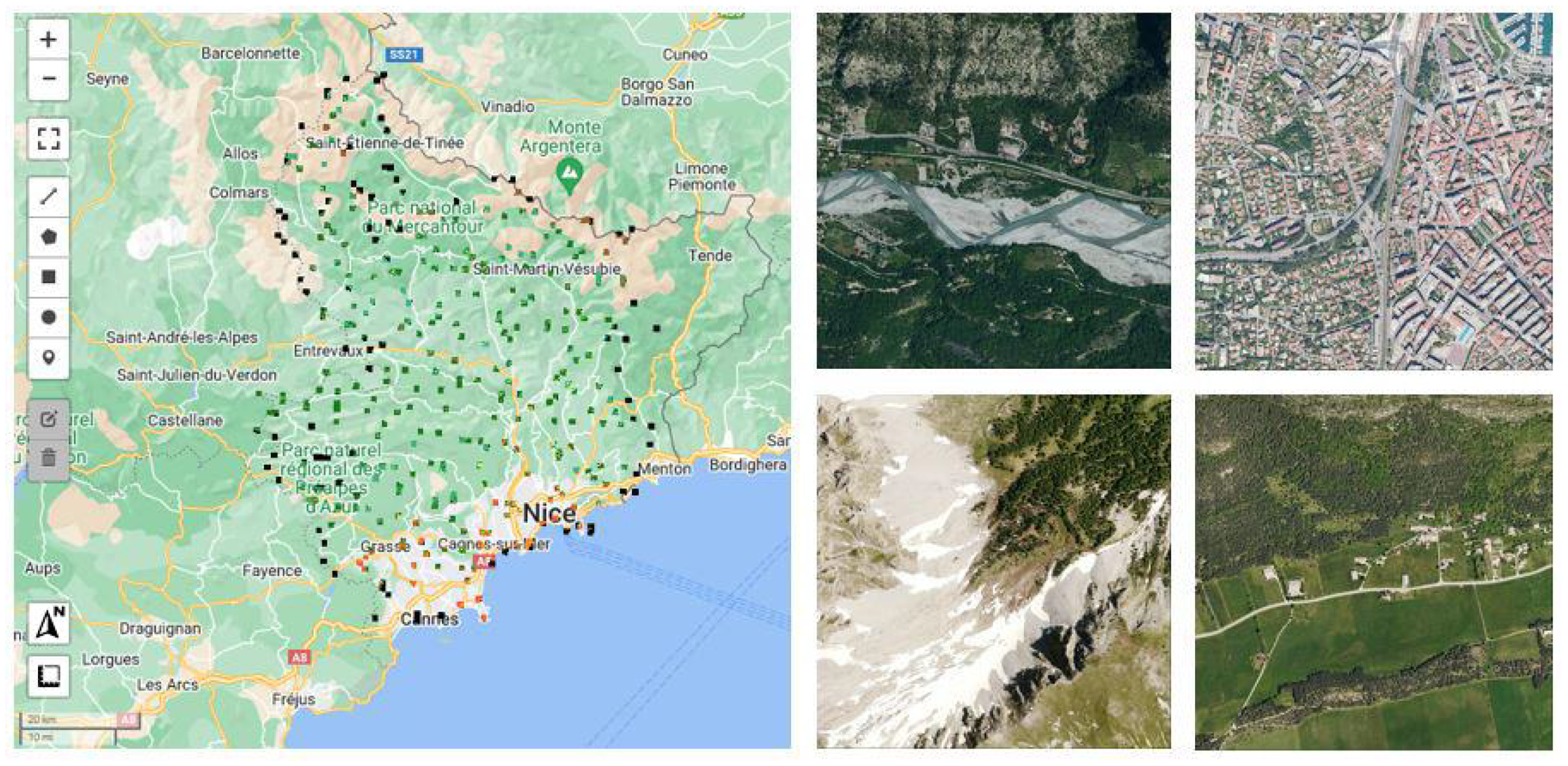
2.1. Study Area

The investigated area comprises the conurbation and the surroundings of Nice, France. It is located on the eastern border with Italy. The image patches are spread out evenly over the area of Nice as shown in Figure 1. The urban area is relatively small; most of the area is covered with forests. The Alps, spanning the border between France and Italy, are characterized by a rough, richly diverse, mountainous area with snow-covered tops.

2.2. Training Data

The very high resolution (VHR) image patches and the labels are part of the grss_dfc_2022 dataset provided by the 2022 IEEE GRSS Data Fusion Contest (DFC2022). The VHR aerial imagery and labels originate from the MiniFrance dataset [25,26]. This is the first dataset for benchmarking semi-supervised learning in the field.

The labels originate from the Urban Atlas 2012, generated by the Copernicus program. Although the labels are generated in 2012, the optical imagery was acquired between 2012 and 2014. The VHR image tiles span $2000\times 2000$ pixels at a resolution of 50 cm/pixel. We limit the investigated area to Nice. The 333 image tiles are spread out evenly over Nice as shown in Figure 1. We integrate Sentinel-2 (S2) data spanning a 3 year period from 2017 to 2019. All 13 bands of the S2 data are retained. The RGB and NIR bands have a resolution of 10 m/pixel; the remaining bands have a resolution of either 20 or 60 m.

Three data sources are used in this study:

• Sentinel-2 imagery
• Very high resolution optical imagery
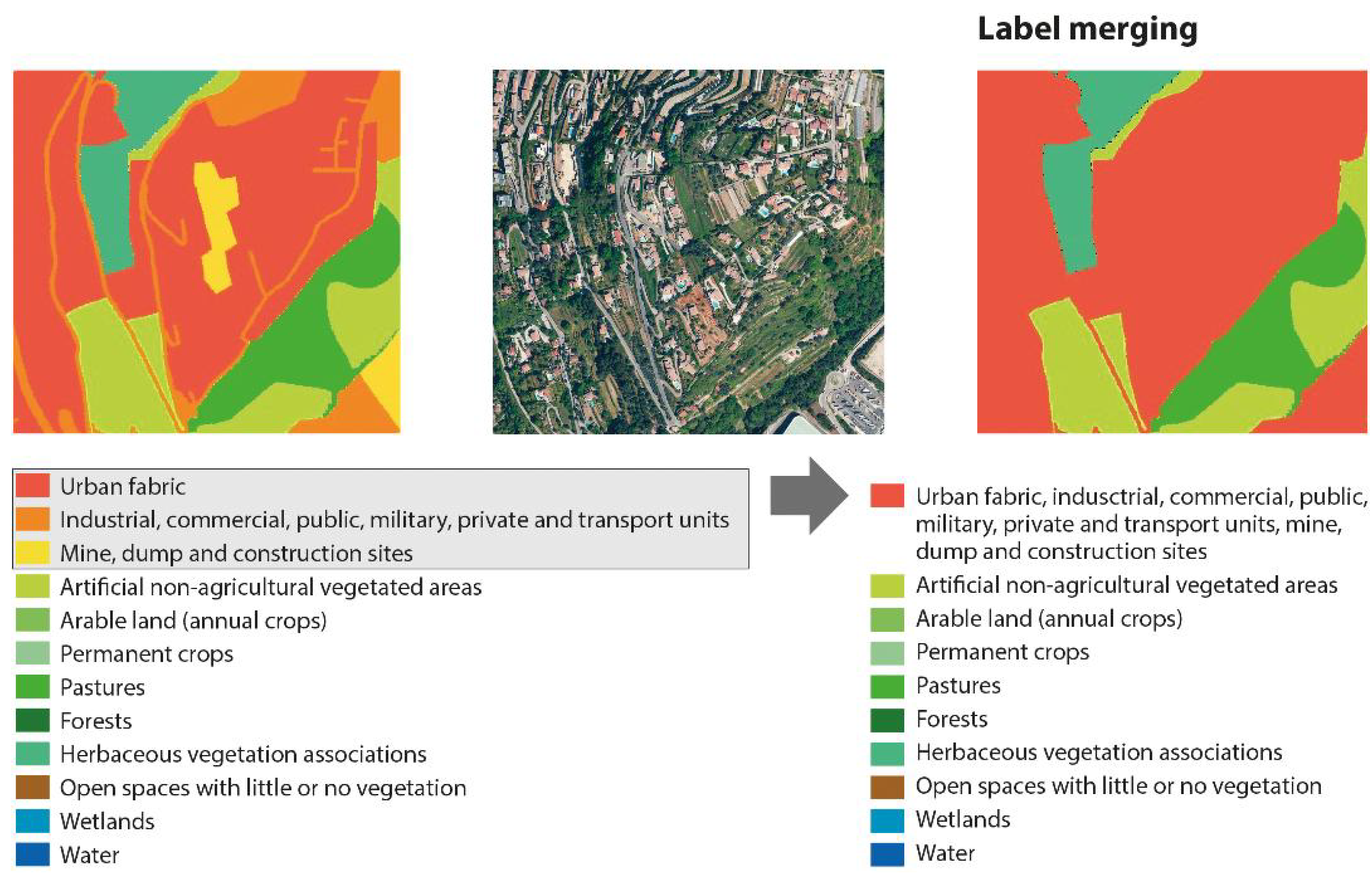
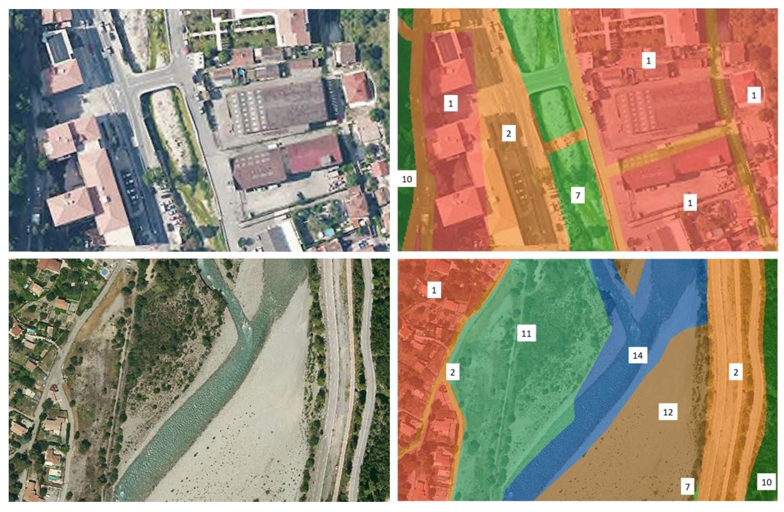
• Land Use/Land Cover labels

The MiniFrance labels contain 14 land cover classes, but in Nice only 9 classes are present. The dataset involves two challenges: a temporal aspect and undetectable classes due to the high resolution of the labels. There are 3 urban classes that cause confusion with the provided VHR aerial imagery and the S2 data: (red label) urban fabric, (orange label) industrial, commercial, public, military, private and transport units, (yellow label) mine, dump and construction sites. The orange label includes roads which are too narrow to be detected in S2 imagery. The yellow label contains construction sites, which are of a temporal nature and might have disappeared in the used S2 imagery. Therefore, we merge these three classes into one urban class. Figure 2 shows how the three urban classes were merged into one class. Finally, we retain 10 classes.

Although the labels are designed to train a convolutional neural network, we choose to extract point samples and train a machine learning model for several reasons. First, the provided labels are not reliable as we will discuss in detail below. Second, we aim to investigate the possibilities of various input data sources using less training data. Deep learning models such as CNNs have performed well for LULC mapping, but require training data that are complex to obtain. To extract training samples, we use a stratified sampling technique, as illustrated in Figure 2. Out of each class, 500 point samples are randomly selected. We split the data into a 400–100 training–validation set. When training the model, we consider a 40 m buffer around each point in case points fall on unclear borders of two classes.

Upon careful examination, we find many labels to be incorrect. As an example, we provide two VHR orthoimages with their respective labels in Figure 3. In the top image, we see that the buildings on the left are labeled partially as class 1 and partially as class 2 due to a straight divide between classes 1 and 2. In the middle on the image, the label of the bridge is misplaced. Furthermore, it is highly unlikely that the middle area running from top to bottom is pasture. In the bottom image, the water class encompasses part of the surrounding dry area. The orange class 2 labels on the left side do not perfectly align with the roads. These two images clearly show that the training samples will be affected by poor labeling and this further motivates us to train an RF classifier instead of a deep learning model.

2.2.1. Spectral Indices

From the S2 bands, we extract 8 spectral indices to provide more information on vegetation, urban cover, bare ground and water classes. A list of the used indices is provided in

Table 1. Spectral indices extracted from Sentinel-2 bands.

Index	Full Name	Formula
BSI [27]	bare soil index	$\frac{(B11+RED)-(NIR+BLUE)}{(B11+RED)+(NIR+BLUE)}$
EVI [28]	enhanced vegetation index	$2.5\frac{NIR-RED}{NIR+6\dot{R}ED-7.5\dot{B}LUE+1}$
GRVI [29]	green-red vegetation index	$\frac{GREEN-RED}{GREEN+RED}$
MNDWI [30]	modified normalized difference water index	$\frac{GREEN-B11}{GREEN+B11}$
NDBI [31]	normalized difference built-up index	$\frac{B11-NIR}{B11+NIR}$
NDVI [32]	normalized difference vegetation index	$\frac{NIR-RED}{NIR+RED}$
NMDI [33]	normalized multi-band drought index	$\frac{NIR-(B11-B12)}{NIR+(B11-B12}$
SMMI [34]	soil moisture monitoring index	$\sqrt{\frac{NIR+B11}{2}}$

.

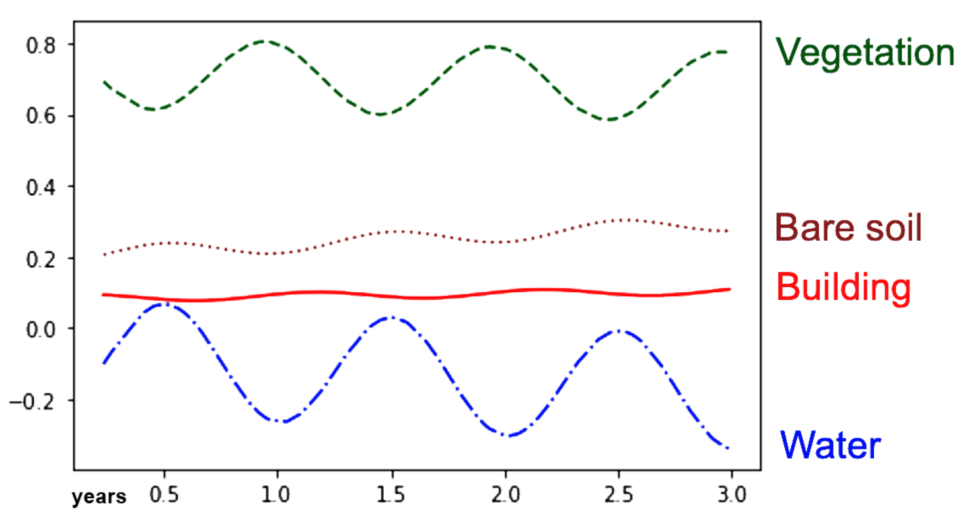
2.2.2. Pixel-Wise Temporal Analysis

Performing a harmonic analysis of satellite data can help in restoring missing data values in a time series, but it can also be used to observe phenology cycles. Extracting the phenology is useful for classifying vegetative land cover classes [8] and distinguishing vegetation with large intra-annual NDVI variations from urban classes with low intra-annual variation [7].

The intra-annual trend of the spectral indices can be approximated using a harmonic function:

$$NDV{I}_t={\beta }_0+{\beta }_{1}t+{\beta }_{2}cos\left(2\pi \omega t\right)+{\beta }_{3}sin\left(2\pi \omega t\right)$$

(1)

where t is the time in decimal years, $\omega$ is the phase ($t_0$ to the first peak) and the ${\beta }^{\prime }s$ are the parameters.

We model the intra-annual trend of five spectral indices (BSI, GVRI, NDBI, NDVI, NMDI) for each pixel in the input image according to the harmonic function. We choose these indices as this subset will be sufficient to identify the classes of the dataset. An example of the fitted harmonic is shown in Figure 4. From the fitted curve, we extract five metrics: maximum, standard deviation, phase, amplitude and mean value. The phase $\omega$ represents the time of year when a vegetation cover matures. The amplitude shows the intra-annual variation. Using phase, amplitude and the mean value, we can construct an HSV image such as Figure 5.

2.3. Random Forest Classifier

The Random Forest (RF) classifier is a machine learning method often used in LULC classification. The benefit of RF is that it is insensitive to overfitting, it is fast to train compared to convolutional neural networks and no normalization of the input data is required [18,22]. Furthermore, the feature importance can easily be determined. The decisions made in the trees can be inspected to help determine which features are most decisive for determining the land cover class.

Regarding the dataset used in this study, RF is especially suitable. The used dataset only contains few labeled samples. In this study, we used 333 tiles out of which we extracted 500 training points per class ($500\times 10=5000$ labeled points). In addition, the provided labels cover challenging classes which results in mislabeled points. Deep learning networks are sensitive to the amount of training data and noisy data. RF will outperform deep learning networks in such cases [22,35]. Given the nature of the data, we choose to train an RF classifier even though the data fusion contest was designed for a deep learning network using semi-supervised learning.

RF is comparable to a Support Vector Machine (SVM). However, Lawrence and Moran [36] found in their classification accuracy comparison tests that RF outperforms SVM: out of 30 datasets, RF was found to be the highest performing classifier. In our initial tests, we found that RF outperformed SVM but only marginally.

Dieu et al. [22] perform hyperparameter tuning to reduce the overfitting of the Random Forest classifier. Because the Random Forest classifier is prone to overfit on a high-dimensional dataset, they limit the number of trees and number of variables in each tree. This reduces the correlation between each tree and guarantees the importance of the variables used in the tree. We choose to limit the number of trees to 25 as increasing it does not improve the performance of the model.

2.4. GEOBIA: Geographic Object-Based Image Analysis

Geographic Object-Based Image Analysis (GEOBIA) is an object-oriented approach to classify pixels in an image. The goal is to extract meaningful objects out of the image and classify these objects as a whole regarding their spectral information as well as their texture. The mean of the individual pixels in the segments is considered as input.

2.4.1. SNIC

To extract the objects, we use Simple Non-Iterative Clustering (SNIC), an unsupervised clustering algorithm that groups neighboring pixels into segments [37]. We perform SNIC using a built-in function in GEE with a compactness of 0 to not limit the shape of the clusters, a connectivity of 8 to include all directions and a neighborhood size of 256 (all following the example from Tassi and Vizzari [24]). For the seeds we use a grid of 10 pixels. As input bands for the clustering, we use all available bands from the composite. Then, to test if clustering improves solely relying on the VHR imagery, we also perform SNIC on only the VHR RGB bands.

2.4.2. GLCM

As a texture index, we use the seven most relevant GLCM metrics extracted from a grey-scale image according to Tassi and Vizzari [24], namely angular second moment, contrast, correlation, entropy, variance, inverse difference moment and sum average. We used the built-in GEE GLCM function with a size of 2 and the default value for kernel (null) and averaging set to True. For each object patch, the mean of the GLCM metric is retained. The value of each GLCM metric is added to the image composite as a new band. The grey scale image is calculated using two formulas. When using the VHR RGB image, the one-band grey-scale image for the GLCM is generated using the blue, red and green band of the VHR image:

$$grey=0.11B+0.3R+0.59G$$

(2)

When extracting textures from the S2 imagery, the following combination of bands is used to create the grey-scale input image:

$$grey=0.11G+0.3NIR+0.59R$$

(3)

3. Results

In this section, we present and discuss the results of our tests. We focus on several research questions which are elaborated in the following subsections. Figure 6 displays some results of the predictions made by the trained Random Forest models. The image shows results for two areas. The left column shows the generated clusters using only the Sentinel-2 bands, the VHR aerial image of that same area and the ground truth labels. The next three columns represent the predictions by the model trained on S2 (Sentinel-2 bands), S2i (Sentinel-2 bands and spectral indices) and S2+ (Sentinel-2 bands, spectral indices and their temporal analysis), both with and without VHR aerial image input bands and with adding both the VHR input bands and the GLCM texture metrics. From the visual results, it is clear that when SNIC is performed on the VHR aerial image bands, the clusters are more refined resulting in a finer prediction. Furthermore, the class predictions differ when adding the VHR aerial image and the GLCM texture metrics. However, the most noticeable difference is in the ground truth labels, which are very smooth and cover large areas with the same class. Fine roads, which cannot be observed in the Sentinel-2 images or SNIC clusters, are also present.

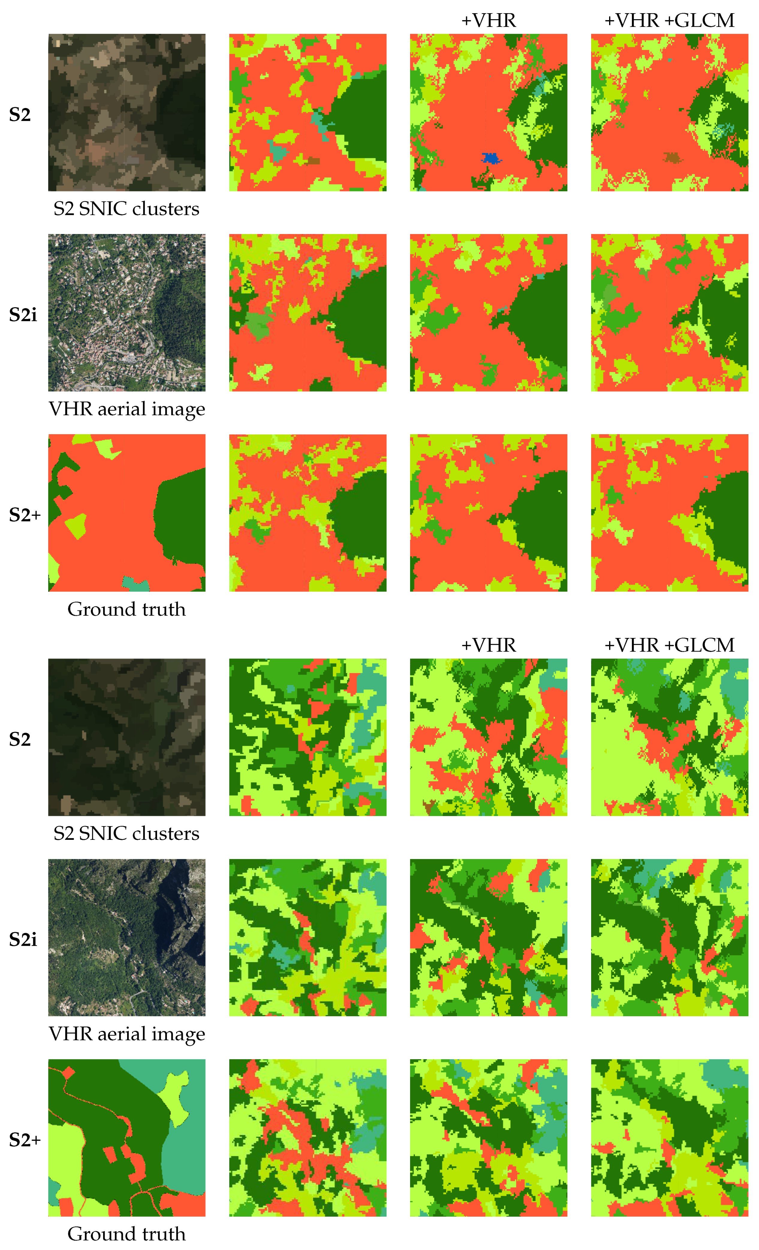
3.1. Improvements Adding the Temporal Analysis

In

Table 2. The overall accuracy (OA) & improvement of the object-based image analysis (GEOBIA) using various input layers.

Input Data	OA	OA Improvement
S2	0.6262
S2i (S2 + indices)	0.6732	+0.0470
S2+ (S2i + temporal analysis)	0.7290	+0.0558

we see that the overall accuracy (OA) of three tests in which the input data are expanded each time, increases with more input bands. Test one (S2) uses the 13 S2 bands as input to the RF classification model and results in an OA of 0.6262. When adding the 8 spectral indices, the OA increases with +0.0470 points. Test S2+ contains the max, standard deviation values and the temporal analysis (phase and amplitude) of 5 spectral indices as well, which improves the OA by the maximum value of +0.0558 compared to the previously mentioned test.

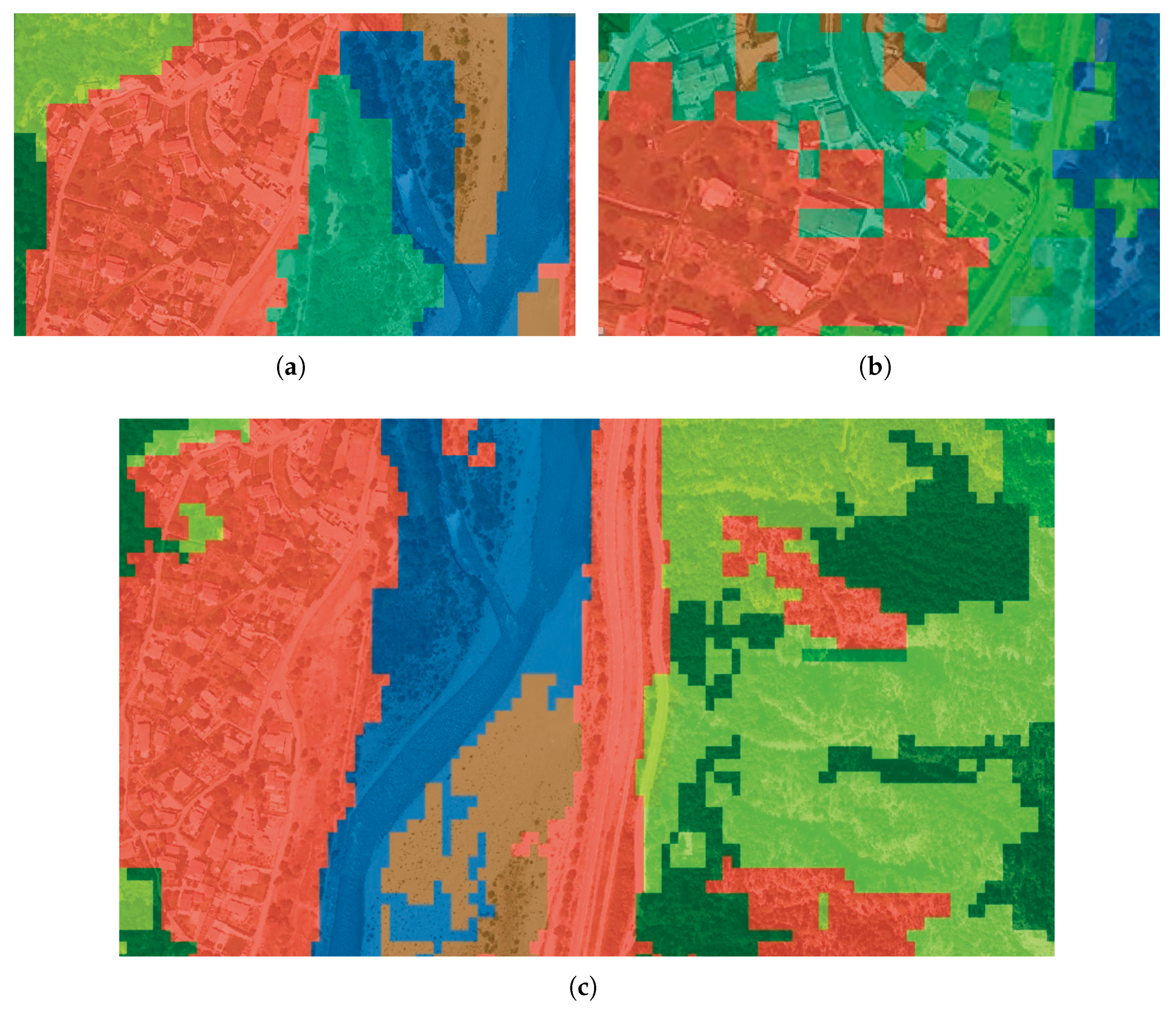
3.2. Improvements Adding One VHR Image

Adding one VHR image can improve the OA as shown in

Table 3. The overall accuracy (OA) improvement adding one VHR image with clustering based on the Sentinel-2 and VHR bands or only on the VHR bands.

Input Data	Base OA	Improvement	With VHR	Clustering on
S2	0.6262	+0.0443	0.6705	S2 and VHR bands
		+0.0934	0.7196	VHR bands
S2i	0.6732	+0.0284	0.7016	S2i and VHR bands
(S2 + indices)		+0.0103	0.6835	VHR bands
S2+	0.7290	+0.0140	0.7430	S2+ and VHR bands
(S2i + temporal analysis)		−0.0127	0.7163	VHR bands

. This effect is most noticeable when only the raw S2 bands are used. The clustering is then best performed on the VHR bands only. When including the spectral indices (S2i), the clustering is best performed on all input bands, i.e., the S2 bands, spectral indices and VHR bands. When including the temporal analysis of the spectral indices (S2+), adding the VHR image does not improve the OA noticeably. On the contrary, the OA decreases for S2+ and VHR input data when clustering only on the VHR bands. In Figure 7, the predictions of three tests are shown: (a) S2 without VHR, (b) S2 with VHR (clustering on the VHR input bands) (c) and S2+ with VHR (clustering on S2+ and VHR bands). Using the VHR input bands to form the clusters, visually refines the clusters. The usage of the SNIC algorithm for clustering on the VHR image can be questioned. It can be argued that this algorithm is not designed to be applied to remote sensing imagery and, therefore, the generated clusters are not optimal. Modern clustering techniques employ deep learning techniques to leverage deep visual features as in [38]. These techniques employ transfer-learned networks that are trained to interpret satellite imagery.

3.3. Improvements Adding the GLCM

The overall accuracy (OA) of the results with the VHR image and the GLCM is shown in

Table 4. The overall accuracy (OA) improvement adding the GLCM with clustering based on various input bands.

Input Data	Base OA	Improvement	OA	With	Clustering on
S2	0.6262	+0.0443	0.6705	VHR	S2 and VHR bands
		+0.0328	0.6590	GLCM	S2 bands
		+0.0414	0.6676	VHR & GLCM	S2 and VHR bands
S2i	0.6732	+0.0284	0.7016	VHR	S2i and VHR bands
(S2 + indices)		+0.0066	0.6798	GLCM	S2i bands
		+0.0536	0.7268	VHR & GLCM	S2i and VHR bands
S2+	0.7290	+0.0140	0.7430	VHR	S2+ and VHR bands
(S2i + temporal analysis)		+0.0032	0.7322	GLCM	S2+ bands
		+0.0076	0.7366	VHR & GLCM	S2+ and VHR bands

. The GLCM is based on the VHR bands when available in the input data. The table compares the OA to the base OA. Adding the VHR leads to a bigger increase of OA than the GLCM. The largest OA is achieved with the S2+ input data with the VHR image. Adding the GLCM does not increase the OA noticeably. In contrast, the VHR image bands or the combination of VHR and GLCM increase the OA by as much as 0.0536. Both Trias-Sanz et al. [21] and Okubo et al. [20] also found that the GLCM did not improve the GEOBIA LULC classification in very high resolution imagery (aerial and QuickBird). Since adding the GLCM to the S2 data has a bigger contribution than when added to the S2i and S2+ data, we can derive that the indices are enough to classify land use at the object level.

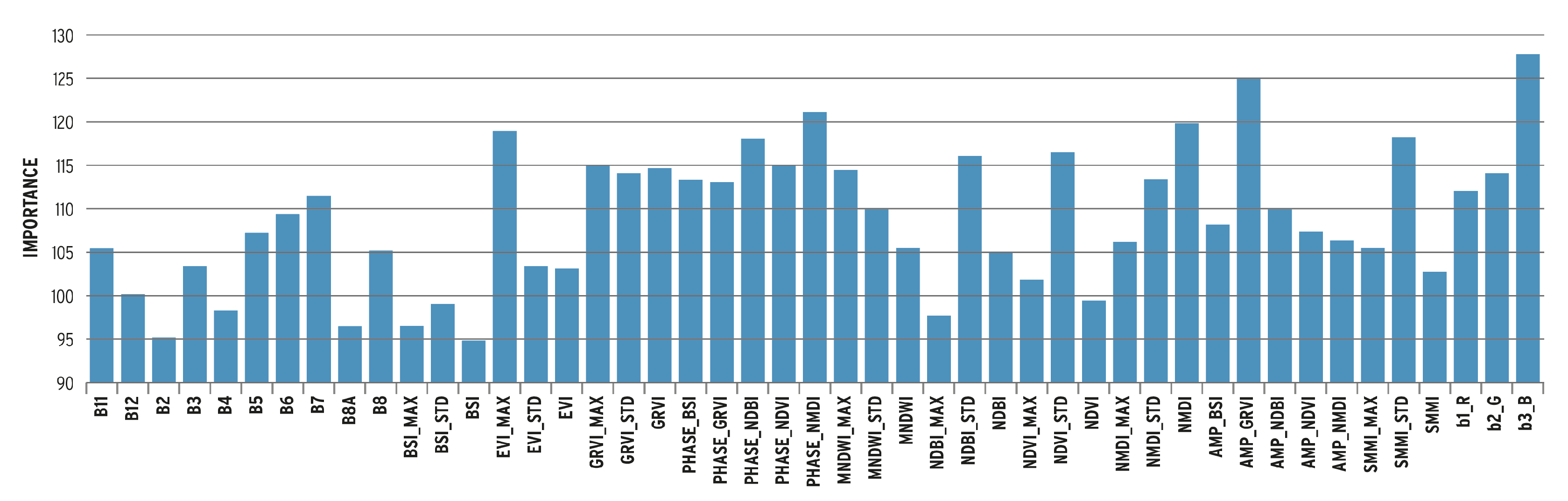
3.4. The Relative Importance Histogram

The highest overall accuracy of 0.7430 is achieved using GEOBIA on S2 data, indices and temporal analysis (S2+) input data with VHR image. The relative importance histogram of the RF model is shown in Figure 8. The higher the bands appear in the trees, the higher their importance. The exact importance measure is determined using the Gini-index. The three VHR bands on the right side in the graph show high relevance to the class prediction, with the blue band b3_B being the most important. Most of the temporal analysis bands show higher relevance than the original S2 bands. Looking at the indices, the GRVI amplitude (AMP_GRVI) is the most important, followed by the NMDI phase (PHASE_NMDI) and the NMDI mean (NMDI). The Sentinel-2 blue band B2 has one of the lowest relative importances likely due to the fact that this information is duplicated in the VHR blue band. The bare soil index bands BSI_MAX, BSI_STD and BSI have very low relative importance. However, the phase and amplitude have high relative importance. These last two represent the time of year an area achieves its highest BSI value and the amount of annual variation in BSI.

Overall, the indices are more important than the raw S2 bands because an index contains more information than a single input band. However, it cannot be concluded that the bands with lower relevance are completely irrelevant because they might contain the same information as another more relevant band or combination of bands in the graph. Performing principal components analysis as described in [24,39] can help in reducing the number of bands by merging those that have equal deterministic properties.

When selecting the 20 most relevant bands (out of 57 for S2+ with VHR and GLCM) and retraining the classifier on these, the OA only drops by 0.01 point. It can thus be concluded that certain bands contain irrelevant or correlated information to the LULC classes.

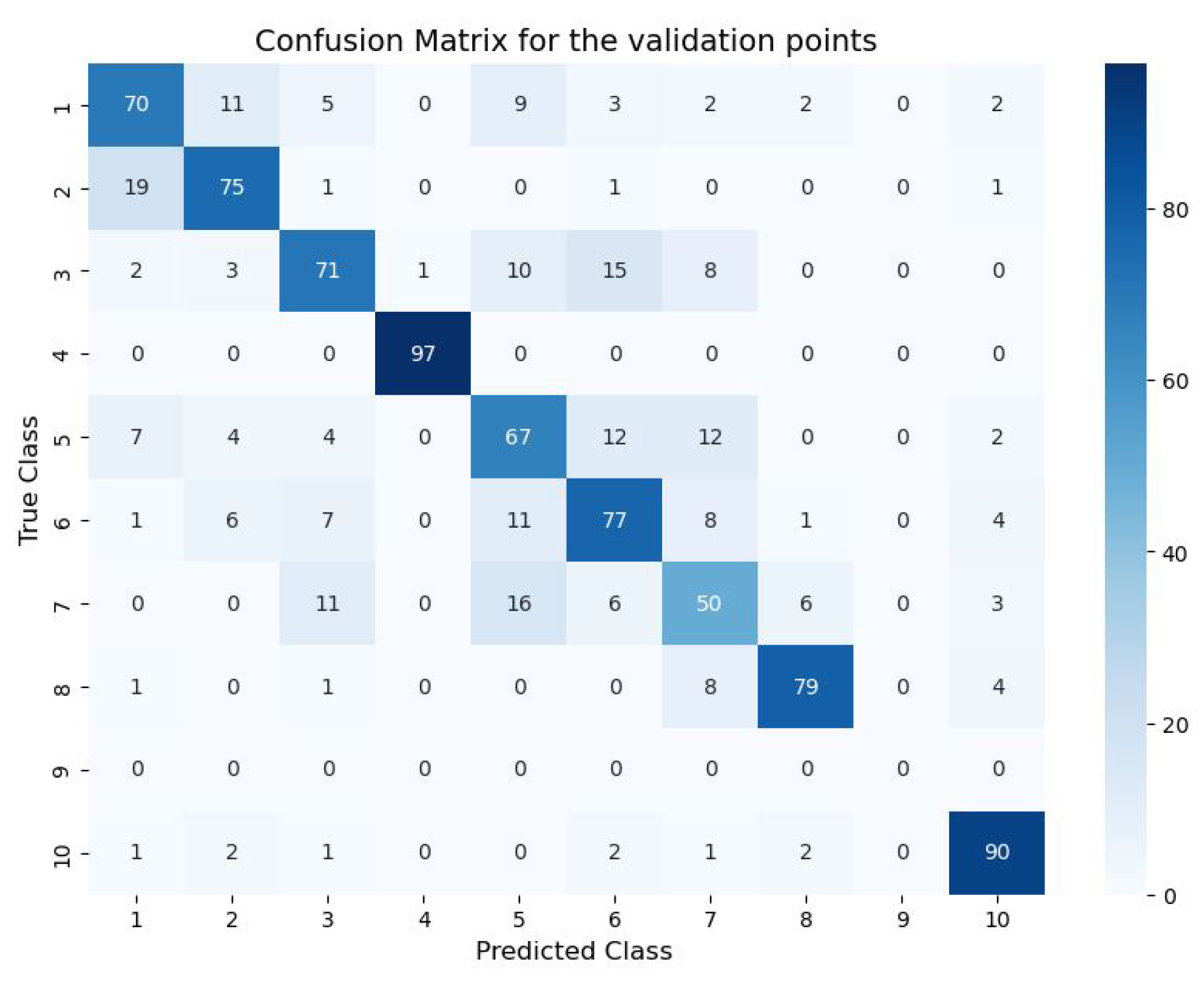
3.5. Confusion Matrix

There are approximately 100 validation samples per LULC class. The confusion matrix (CM) for S2+ with VHR image bands is shown in Figure 9. Class 9 is absent in the study area. The CM shows confusion between classes 1 and 2 and classes 5, 6 and 7. Class 1 represents urban areas and class 2 contains artificial non-agricultural vegetated areas, i.e., parks in urban areas. Due to the difficulty of labeling these classes, the confusion is understandable. Class 5 are pastures, class 6 are forests and class 7 are herbaceous vegetation associations. The intersection over union (IoU) of class 7 is 0.3817. Poor labeling as shown in Figure 2 is to blame for these class confusions.

4. Discussion

The accurate mapping of LULC faces a range of challenges. The class confusion and unclear boundaries in combination with low resolution satellite imagery make it hard to train a general model. Moreover, the available data sources for LULC mapping are diverse, including the temporal aspect which adds complexity and depth to the input data layers. To interpret and limit the various layers of satellite imagery, it is necessary to investigate which parameters are most meaningful for the classification task. To this end, this study integrates two data sources for LULC mapping: multi-temporal and multi-spectral Sentinel-2 data and very high resolution optical imagery. We examine the relevance of different layers for accurate classification using a GEOBIA approach with an unsupervised clustering method following [24]. While Tassi and Vizarri’s work reaches similar conclusions, their study uses only satellite imagery without temporal analysis of indices and is limited to six LULC classes. Furthermore, the labels in their study are generated manually, which could explain the higher accuracy.

Our results show that a Random Forest classifier, combined with the multi-temporal and multi-spectral aspect of Sentinel-2 data, can achieve high accuracy with the MiniFrance dataset. Compared to the supervised and semi-supervised deep learning models used in [25] on the same dataset, our method outperforms with an overall accuracy of 74.30%. The authors of MiniFrance obtained lower overall accuracy of 46.30% and 47.90% for supervised and semi-supervised convolutional neural networks (CNNs), respectively, despite using more training data than we did. The superior performance of our method can be attributed to the use of very high resolution optical imagery to generate object clusters and the incorporation of temporal analysis to identify the phenology of the vegetation.

CNNs have gained popularity in LULC classification research. However, boundary detection is a significant challenge for CNNs. To overcome this, the authors of [40] employed a boundary detection network to fuse the results with the semantic segmentation by a CNN. In a similar manner, our method utilizes clustering to group pixels into objects, which are then used in the classification. Another study compared the performance of a CNN to traditional machine learning models such as Random Forest and super vector machine and found that that the CNN outperformed the machine learning models, especially in identifying coastal regions [41]. However, this approach required manually labeled data and was limited to only five classes, highlighting the need for high-quality data with accurate labeling for effective implementation of CNNs in LULC classification.

Overall, our study suggests that the choice of classification method depends on the availability and quality of the training data. While deep learning CNNs have shown high accuracy in LULC classification, they require large amounts of high-quality labeled data. In cases where training data is limited or unreliable, a Random Forest classifier can still provide a viable alternative with comparable accuracy. This is exemplified by our results, which show that our approach outperforms the deep learning CNN trained on the same dataset [25]. In fact, the authors of [42] mention the MiniFrance dataset, but choose to create a new dataset employing second-level CORINE (Coordination of information on the environment) classes as labels.

5. Conclusions

In this study, we investigate the effectiveness of a Random Forest classifier for land use/land cover mapping in Nice, France. Our method utilizes multi-temporal Sentinel-2 data and a single VHR optical aerial image to improve object recognition in a geographic object-based image analysis (GEOBIA) framework. Specifically, we employ unsupervised clustering with SNIC to generate objects and create eight spectral indices from the Sentinel-2 data. Additionally, we perform a pixel-wise harmonic analysis on the multi-temporal layers of Sentinel-2 data to extract phenological characteristics of the vegetation.

Despite the challenges posed by the dataset, we were able to achieve an overall accuracy of 74.30% by combining the indices and their temporal analysis with the RGB bands of a VHR image. The accuracy of the classification increases from 62.62% when using only the Sentinel-2 bands, to 67.05% upon adding one VHR image. Our analysis reveals that the GLCM texture features do not have a significant impact on the predictions and the VHR image has a greater impact than the GLCM. Notably, the impact of the VHR image is more pronounced when the temporal analysis features and spectral indices are not used. We identify class confusions through the confusion matrix. Moreover, the relative importance histogram indicates that the VHR image bands play a crucial role in accurately predicting the LULC class, highlighting the importance of integrating VHR imagery into the classification process.

Future prospects include the improvement of the generated objects. While we used SNIC clustering in our study, the recently released Segment Anything Model (SAM) [43] generates meaningful objects that can be more accurately classified via machine learning models or even deep learning CNNs. Another promising research area is the integration of GEOBIA methods with deep learning CNNs. By combining the strengths of these two techniques, we may be able to improve our LULC classification accuracy even further. In addition, we can use the relative importance histogram from our study to select the most relevant input layers for training the CNN, which could result in a more efficient and accurate classification process.

Although we have shown the added accuracy resulting from employing various input sources, especially the spectral indices and their temporal analysis, the biggest limitation is by far the used dataset, which also allowed for another aspect of the research, i.e., how to deal with poor data.

References

1. Vermeiren, K.; Crols, T.; Uljee, I.; Nocker, L.D.; Beckx, C.; Pisman, A.; Broekx, S.; Poelmans, L. Modelling urban sprawl and assessing its costs in the planning process: A case study in Flanders, Belgium. Land Use Policy 2022, 113, 105902. [Google Scholar] [CrossRef]
2. Clerici, N.; Calderón, C.A.V.; Posada, J.M. Fusion of sentinel-1a and sentinel-2A data for land cover mapping: A case study in the lower Magdalena region, Colombia. J. Maps 2017, 13, 718–726. [Google Scholar] [CrossRef]
3. Luca, G.D.; Silva, J.M.N.; Fazio, S.D.; Modica, G. Integrated use of Sentinel-1 and Sentinel-2 data and open-source machine learning algorithms for land cover mapping in a Mediterranean region. Eur. J. Remote Sens. 2022, 55, 52–70. [Google Scholar] [CrossRef]
4. Abdi, A.M. Land cover and land use classification performance of machine learning algorithms in a boreal landscape using Sentinel-2 data. GIScience Remote Sens. 2020, 57, 1–20. [Google Scholar] [CrossRef]
5. Erasmi, S.; Twele, A. Regional land cover mapping in the humid tropics using combined optical and SAR satellite data—A case study from Central Sulawesi, Indonesia. Int. J. Remote Sens. 2009, 30, 2465–2478. [Google Scholar] [CrossRef]
6. Xu, L.; Herold, M.; Tsendbazar, N.E.; Masiliūnas, D.; Li, L.; Lesiv, M.; Fritz, S.; Verbesselt, J. Time series analysis for global land cover change monitoring: A comparison across sensors. Remote Sens. Environ. 2022, 271, 112905. [Google Scholar] [CrossRef]
7. Lawton, M.N.; Martí-Cardona, B.; Hagen-Zanker, A. Urban growth derived from landsat time series using harmonic analysis: A case study in south england with high levels of cloud cover. Remote Sens. 2021, 13, 3339. [Google Scholar] [CrossRef]
8. Padhee, S.K.; Dutta, S. Spatio-Temporal Reconstruction of MODIS NDVI by Regional Land Surface Phenology and Harmonic Analysis of Time-Series. GISci. Remote Sens. 2019, 56, 1261–1288. [Google Scholar] [CrossRef]
9. Blaschke, T.; Hay, G.J.; Kelly, M.; Lang, S.; Hofmann, P.; Addink, E.; Feitosa, R.Q.; van der Meer, F.; van der Werff, H.; van Coillie, F.; et al. Geographic Object-Based Image Analysis—Towards a new paradigm. ISPRS J. Photogramm. Remote Sens. 2014, 87, 180–191. [Google Scholar] [CrossRef]
10. Chen, Y.; Ge, Y.; Heuvelink, G.B.; An, R.; Chan, Y. Object-based superresolution land-cover mapping from remotely sensed imagery. IEEE Trans. Geosci. Remote Sens. 2018, 56, 328–340. [Google Scholar] [CrossRef]
11. Sameen, M.I.; Pradhan, B.; Aziz, O.S. Classification of very high resolution aerial photos using spectral-spatial convolutional neural networks. J. Sens. 2018, 2018, 7195432. [Google Scholar] [CrossRef]
12. Mboga, N.; Georganos, S.; Grippa, T.; Lennert, M.; Vanhuysse, S.; Wolff, E. Fully convolutional networks and geographic object-based image analysis for the classification of VHR imagery. Remote Sens. 2019, 11, 597. [Google Scholar] [CrossRef]
13. Gavankar, N.L.; Ghosh, S.K. Object based building footprint detection from high resolution multispectral satellite image using K-means clustering algorithm and shape parameters. Geocarto Int. 2019, 34, 626–643. [Google Scholar] [CrossRef]
14. Praticò, S.; Solano, F.; Fazio, S.D.; Modica, G. Machine learning classification of mediterranean forest habitats in google earth engine based on seasonal sentinel-2 time-series and input image composition optimisation. Remote Sens. 2021, 13, 586. [Google Scholar] [CrossRef]
15. Gudmann, A.; Csikós, N.; Szilassi, P.; Mucsi, L. Improvement in satellite image-based land cover classification with landscape metrics. Remote Sens. 2020, 12, 3580. [Google Scholar] [CrossRef]
16. Polykretis, C.; Grillakis, M.G.; Alexakis, D.D. Exploring the impact of various spectral indices on land cover change detection using change vector analysis: A case study of Crete Island, Greece. Remote Sens. 2020, 12, 319. [Google Scholar] [CrossRef]
17. Haralick, R.M. Statistical and structural approaches to texture. Proc. IEEE 1979, 67, 786–804. [Google Scholar] [CrossRef]
18. Numbisi, F.N.; Coillie, F.M.B.V.; Wulf, R.D. Delineation of Cocoa Agroforests Using Multiseason Sentinel-1 SAR Images: A Low Grey Level Range Reduces Uncertainties in GLCM Texture-Based Mapping. ISPRS Int. J. Geo-Inf. 2019, 8, 179. [Google Scholar] [CrossRef]
19. Su, W.; Li, J.; Chen, Y.; Liu, Z.; Zhang, J.; Low, T.M.; Suppiah, I.; Hashim, S.A.M. Textural and local spatial statistics for the object-oriented classification of urban areas using high resolution imagery. Int. J. Remote Sens. 2008, 29, 3105–3117. [Google Scholar] [CrossRef]
20. Okubo, S.; Muhamad, D.; Harashina, K.; Takeuchi, K.; Umezaki, M. Land use/cover classification of a complex agricultural landscape using single-dated very high spatial resolution satellite-sensed imagery. Can. J. Remote Sens. 2010, 36, 722–736. [Google Scholar] [CrossRef]
21. Trias-Sanz, R.; Stamon, G.; Louchet, J. Using colour, texture and hierarchial segmentation for high-resolution remote sensing. ISPRS J. Photogramm. Remote Sens. 2008, 63, 156–168. [Google Scholar] [CrossRef]
22. Dieu, T.; Le, H.; Pham, L.H.; Dinh, Q.T.; Thuy, N.T. Rapid method for yearly LULC classification using Random Forest and incorporating time-series NDVI and topography: A case study of Thanh Hoa province, Vietnam and topography: A case study of Thanh Hoa. Geocarto Int. 2022, 37, 17200–17215. [Google Scholar] [CrossRef]
23. Walker, K.; Moscona, B.; Jack, K.; Jayachandran, S.; Kala, N.; Pande, R.; Xue, J.; Burke, M. Detecting Crop Burning in India using Satellite Data. arXiv 2022, arXiv:2209.10148. [Google Scholar]
24. Tassi, A.; Vizzari, M. Object-oriented lulc classification in google earth engine combining snic, glcm and machine learning algorithms. Remote Sens. 2020, 12, 3776. [Google Scholar] [CrossRef]
25. Castillo-Navarro, J.; Saux, B.L.; Boulch, A.; Audebert, N.; Lefèvre, S. Semi-Supervised Semantic Segmentation in Earth Observation: The MiniFrance Suite, Dataset Analysis and Multi-Task Network Study; Springer: New York, NY, USA, 2022; Volume 111, pp. 3125–3160. [Google Scholar] [CrossRef]
26. Hänsch, R.; Persello, C.; Vivone, G.; Navarro, J.C.; Boulch, A.; Lefevre, S.; Saux, B.L. The 2022 IEEE GRSS Data Fusion Contest: Semisupervised Learning [Technical Committees]. IEEE Geosci. Remote Sens. Mag. 2022, 10, 334–337. [Google Scholar] [CrossRef]
27. Diek, S.; Fornallaz, F.; Schaepman, M.E.; De Jong, R. Barest Pixel Composite for Agricultural Areas Using Landsat Time Series. Remote Sens. 2017, 9, 1245. [Google Scholar] [CrossRef]
28. Villamuelas, M.; Fernández, N.; Albanell, E.; Gálvez-Cerón, A.; Bartolomé, J.; Mentaberre, G.; López-Olvera, J.R.; Fernández-Aguilar, X.; Colom-Cadena, A.; López-Martín, J.M.; et al. The Enhanced Vegetation Index (EVI) as a proxy for diet quality and composition in a mountain ungulate. Ecol. Indic. 2016, 61, 658–666. [Google Scholar] [CrossRef]
29. Tucker, C.J. Red and photographic infrared linear combinations for monitoring vegetation. Remote Sens. Environ. 1979, 8, 127–150. [Google Scholar] [CrossRef]
30. Xu, H. Modification of normalised difference water index (NDWI) to enhance open water features in remotely sensed imagery. Int. J. Remote Sens. 2006, 27, 3025–3033. [Google Scholar] [CrossRef]
31. Zha, Y.; Gao, J.; Ni, S. Use of normalized difference built-up index in automatically mapping urban areas from TM imagery. Int. J. Remote Sens. 2003, 24, 583–594. [Google Scholar] [CrossRef]
32. Rouse, J.W.; Haas, R.H.; Schell, J.A.; Deering, D.W. Monitoring vegetation systems in the Great Plains with ERTS. NASA Spec. Publ. 1974, 351, 309. [Google Scholar]
33. Wang, L.; Qu, J.J. NMDI: A normalized multi-band drought index for monitoring soil and vegetation moisture with satellite remote sensing. Geophys. Res. Lett. 2007, 34, L20405. [Google Scholar] [CrossRef]
34. Liu, Y.; Qian, J.; Yue, H. Comprehensive Evaluation of Sentinel-2 Red Edge and Shortwave-Infrared Bands to Estimate Soil Moisture. IEEE J. Sel. Top. Appl. Earth Obs. Remote Sens. 2021, 14, 7448–7465. [Google Scholar] [CrossRef]
35. Bai, T.; Sun, K.; Deng, S.; Li, D.; Li, W.; Chen, Y. Multi-scale hierarchical sampling change detection using Random Forest for high-resolution satellite imagery. Int. J. Remote Sens. 2018, 39, 7523–7546. [Google Scholar] [CrossRef]
36. Lawrence, R.L.; Moran, C.J. The AmericaView classification methods accuracy comparison project: A rigorous approach for model selection. Remote Sens. Environ. 2015, 170, 115–120. [Google Scholar] [CrossRef]
37. Achanta, R.; Süsstrunk, S. Superpixels and polygons using simple non-iterative clustering. In Proceedings of the 30th IEEE Conference on Computer Vision and Pattern Recognition, CVPR 2017, Honolulu, HI, USA, 21–26 July 2017; pp. 4895–4904. [Google Scholar] [CrossRef]
38. Gargees, R.S.; Scott, G.J. Deep Feature Clustering for Remote Sensing Imagery Land Cover Analysis. IEEE Geosci. Remote Sens. Lett. 2020, 17, 1386–1390. [Google Scholar] [CrossRef]
39. Hall-Beyer, M. Practical guidelines for choosing GLCM textures to use in landscape classification tasks over a range of moderate spatial scales. Int. J. Remote Sens. 2017, 38, 1312–1338. [Google Scholar] [CrossRef]
40. Xu, Z.; Su, C.; Zhang, X. A semantic segmentation method with category boundary for Land Use and Land Cover (LULC) mapping of Very-High Resolution (VHR) remote sensing image. Int. J. Remote Sens. 2021, 42, 3146–3165. [Google Scholar] [CrossRef]
41. Xie, G.; Niculescu, S. Mapping and monitoring of land cover/land use (LCLU) changes in the crozon peninsula (Brittany, France) from 2007 to 2018 by machine learning algorithms (support vector machine, Random Forest and convolutional neural network) and by post-classification comparison (PCC). Remote Sens. 2021, 13, 3899. [Google Scholar] [CrossRef]
42. Sertel, E.; Ekim, B.; Osgouei, P.E.; Kabadayi, M.E. Land Use and Land Cover Mapping Using Deep Learning Based Segmentation Approaches and VHR Worldview-3 Images. Remote Sens. 2022, 14, 4558. [Google Scholar] [CrossRef]
43. Kirillov, A.; Mintun, E.; Ravi, N.; Mao, H.; Rolland, C.; Gustafson, L.; Xiao, T.; Whitehead, S.; Berg, A.C.; Lo, W.Y.; et al. Segment Anything. arXiv 2023, arXiv:2304.02643. [Google Scholar]
Figure 1. The area of Nice is located on the Mediterranean Sea coast of southeastern France. All available image patches are shown on the left map. Four examples of the orthoimages are shown on the right. Each tile encompasses 1 km 2 .
Remotesensing 15 02501 g001
Figure 2. The 12 available classes in the IEEE data fusion contest is reduced to ten. Training samples are acquired through stratified point sampling.
Remotesensing 15 02501 g002
Figure 3. Poor data labeling by the Urban Atlas and reused in the IEEE data fusion contest. (Left) aerial imagery. (Right) labeled images. The labels are as follows: 1: Urban fabric; 2: Industrial, commercial, public, military, private and transport units; 7: Pastures; 10: Forests; 11: Herbaceous vegetation associations; 12: Open spaces with little or no vegetation; and 14: Water.
Remotesensing 15 02501 g003
Figure 4. The fitted harmonic trend of NDVI at four different locations. Land cover classes can be distinguished based on the fitted curves. To include this information in the image composite, the maximum value, standard deviation, phase, amplitude and mean value of each curve are added as bands.
Remotesensing 15 02501 g004
Figure 5. The HSV image shows the phase (HUE), amplitude (SAT) and mean (VAL) of the NDVI index in a region at the coast of Nice. The color indicates at what time of year a crop matures. The saturation shows how much intra-annual variation is observed. Black areas have a low mean value and thus no variation is present.
Remotesensing 15 02501 g005
Figure 6. The resulting LULC Random Forest prediction for two VHR aerial images using Sentinel-2 input data (S2), spectral indices (S2i) and the temporal analysis (S2+). In the third column, the VHR orthoimage is added. In the last column, the GLCM features are added. For the legend, we refer to Figure 2.
Remotesensing 15 02501 g006
Figure 7. The predictions are influenced by the clustering. (a) Clustering on S2 data, prediction on S2. (b) Clustering on VHR, prediction on S2 and VHR. (c) Clustering on S2+ and VHR, prediction on S2+ and VHR.
Remotesensing 15 02501 g007
Figure 8. The relative importance histogram of S2+ with VHR image bands. The 12 S2 bands are shown on the left. The middle section shows the spectral indices and their temporal analysis bands. The VHR bands are on the outer right. In general, the VHR bands have a high relevance meaning that they have the highest Gini-index in the random forest.
Remotesensing 15 02501 g008
Figure 9. The confusion matrix of S2+ with VHR image bands.
Remotesensing 15 02501 g009