Abstract
Land cover classification in semiarid areas is a difficult task that has been tackled using different strategies, such as the use of normalized indices, texture metrics, and the combination of images from different dates or different sensors. In this paper we present the results of an experiment using three sensors (Sentinel-1 SAR, Sentinel-2 MSI and LiDAR), four dates and different normalized indices and texture metrics to classify a semiarid area. Three machine learning algorithms were used: Random Forest, Support Vector Machines and Multilayer Perceptron; Maximum Likelihood was used as a baseline classifier. The synergetic use of all these sources resulted in a significant increase in accuracy, Random Forest being the model reaching the highest accuracy. However, the large amount of features (126) advises the use of feature selection to reduce this figure. After using Variance Inflation Factor and Random Forest feature importance, the amount of features was reduced to 62. The final overall accuracy obtained was 0.91 ± 0.005 ( = 0.05) and kappa index 0.898 ± 0.006 ( = 0.05). Most of the observed confusions are easily explicable and do not represent a significant difference in agronomic terms.
1. Introduction
Semi-arid Mediterranean regions are extremely challenging for land cover classification using remote sensing imagery. The reason is the landscape’s high spatial irregularity related to specific socio-economic and physical characteristics. This irregularity includes a high variety of spatial patterns, a strong fragmentation and a wide range of vegetation coverages [1]. Distinction between crops and natural vegetation, rain-fed and irrigated crops, or between some anthropogenic surfaces is a complex and difficult issue to solve, hindered by the diverse spectral properties of rocks and soils and by the diverse biophysical characteristics of plant species.
This issue has been addressed by using indices derived from reflectivity that emphasize different biophysical characteristics of the surface [2]. Other derived information such as texture [1] has also been used to increase classification accuracy. Some descriptive statistics derived from the Grey Level Co-occurrence Matrix (GLCM) [3] are the most extended texture features used for classification purposes [4,5]. Multi-temporal classification approaches have also been used to improve accuracy, as it means the inclusion of a wider range of information related to phenology, biophysical state and temporal evolution of crops and natural vegetation [6,7,8,9].
Synthetic Aperture Radar (SAR) backscatter intensity information from co- and cross-polarized channels has proven to be useful to identify different types of crops or biophysical parameters such as plant phenology and morphology in many recent studies [10,11,12]. Metrics derived from SAR data as the ratio cross-/co-polarization have been also tested in several studies to retrieve biophysical parameters for crop classification [6,13]. Soil moisture, roughness and topography have been shown to affect the surface backscatter [14]; hence SAR data may be also considered a proxy for other ancillary information. Other indices derived from SAR polarizations, such as the Dual Polarization SAR Vegetation Index (DPSVI) developed by [15], aim to separate bare soil from vegetation. SAR imagery is being used currently for crop classification because it may provide information on soil moisture, biomass or crop growth. Additionally, it has the advantage that is not affected by either cloud coverage or the satellite passage time.
The Sentinel program from the European Spatial Agency (ESA) includes specific satellites focusing on many different aspects of Earth observation, including land monitoring. Sentinel-1 (S1) and Sentinel-2 (S2) are two constellations of twin-polar orbiting satellites launched between 2014 and 2018. Their combined use allows high temporal resolution to be achieved.
S1A and S1B operates in a C-band SAR, imaging day and night in all weather conditions with the C-SAR instrument in four different modes, with variable resolution ranging down to 5 m, and a coverage area up to 400 km. Revisit time combining ascending and descending modes from both satellites is about a couple of days over Europe, achieving a global coverage every two weeks. One of the four modes of acquisition of the reflected signal is the Interferometric Wide-Swath (IW) mode, in which co- (VV) and cross- (VH) polarization backscatter intensity values are obtained. The utility of Sentinel-1 SAR time series for crop monitoring has been stated in several studies [11,12,16,17].
S2A and S2B contain a Multi-Spectral Instrument (MSI), an optical (passive) system that samples 13 spectral bands from visible, near-infrared and short-wave infrared. They have high temporal resolution (revisit time of 5 days at equator and 2–3 days under cloud-free conditions in mid-latitudes) and high spatial resolution (10 m in the visible and near-infrared spectra). Their data have already been tested in land cover classification and biophysical parameters estimation [18,19,20] with good results due to their temporal and spatial resolution, which is better than Landsat, but at the same time is completely interoperable with it [21].
In recent years, there has been an increasing trend towards the synergetic usage of optical and SAR data in land cover classification. Denize et al. [6] used S1 and S2 to better identify winter land use in a small study area in northern France because of the independence of SAR from atmospheric conditions. Campos et al. [7] classified land cover using S1 and S2 in a study area, similar to ours both environmentally and in size. In some cases segmentation was also included in the classification workflow [22]. The temporal evolution of imagery from both sensors has also been used to improve land cover classification [14]. Other studies used higher-resolution imagery combinations of multispectral and SAR in smaller areas, even using time series [13]. Some studies focused on some specific land covers or environments; for example, Haas et al. [23] or Tavares et al. [24] combined S1 and S2 to map urban ecosystem services, and Amoakoh et al. [25] to classify land cover in a peatland in Ghana.
Some studies demonstrate the significant improvement when using machine learning (ML) methods for classification. Masiza et al. [26] compared Xgboost, Random Forest (RF), Support Vector Machines (SVM), Neural Networks and Naive Bayes to classify the S1 and S2 combination in small farming areas. Dobrinić et al. [27] used machine learning methods (RF and Extreme Gradient Boosting) for land cover classification in Lyon (France), increasing overall accuracy from 85% to 91%, significantly improving classification in urban areas and reducing confusions between forest and low vegetation. De Luca et al. [28] studied the integration of both sensors using RF in a heterogeneous Mediterranean forest area, including time-series of each SAR and optical bands and spectral indices; they obtained an overall accuracy of 90% and the integration of SAR improved by 2.53%, which was obtained using only optical data. Zhang et al. [9] studied the differences in temporal signatures between vegetation cover types, combining three types of temporal information of S1 and S2 using the SVM classifier. De Fioravante et al. [29] proposed a land cover classification methodology for Italy based on decision rules using the EAGLE-compliant classification system [30], obtaining an overall accuracy of 83%, which seems to be much lower than those obtained using machine learning. Most recent and innovative research includes further comparisons with methods of Deep Learning and Artificial Neural Networks, as in [31] or [32].
The synergetic use of optical and SAR data has already proven its utility also in mapping and classifying different types and stages of crops [33], as well as some different agricultural practices [34] or problems in crops growing [35]. It has also proven useful in forest applications. Andalibi et al. [36] used S2, Landsat8, MODIS and AVHRR to estimate the plant canopy Leaf Area Index. Zhang et al. [37] integrated topography indices with S1 and S2 to estimate forest height using different machine learning algorithms. Guerra Hernandez et al. [38] mapped above-ground biomass by integrating ICESat-2, S1, S2, ALOS2/PALSAR2, and topographic information in Mediterranean forests. Kabisch et al. [39] combined Landsat, S2, and RapidEye to analyze land use change in urban areas.
Recently, Light detection and ranging (LiDAR) data are being increasingly used in an integrated manner with multispectral information and radar in land cover analysis. The availability of accurate information about the height of objects such as trees or buildings may improve the accuracy of the resulting metrics. It has been used to map forest coverage metrics. For instance, Heinzel et al. [40] combined LiDAR and high-resolution CIR imagery to identify trees in a small study area. Montesano et al. [41] used Landsat, SAR and LiDAR to improve the estimation of forest biomass. More recently, Chen et al. [42], Morin et al. [43] or Torres de Almeida et al. [44] combined S1, S2 and LiDAR to estimate forest aboveground biomass. Spectral and LiDAR information have also been combined to analyze urban areas [45,46]. Rittenhouse et al. [47] combined Landsat, LiDAR and aerial imagery to estimate forest metrics with which to establish a forest classification.
Since the launch of new satellites such as GEDI or ICEsat2, the availability of remote LiDAR data has increased, providing another source of information that is being increasingly used to complement multispectral and other derived variables, mainly to map forest coverage metrics [42,43,48].
One of the conclusions that can be drawn from these studies is that the more sources, the better results. However, an increase in the number of sources indeed increases the dimensionality of the problem, so feature selection based on importance [49,50] or comparing different subsets extracted from the main data [44] is usually performed
Although S1 and S2 have been previously combined to improve land cover classification accuracy, the inclusion of LiDAR metrics in the feature dataset has been mainly focused to the estimation of specific metrics in specific environments such as forest, agricultural and urban areas. The aim of this study was to find out whether a synergetic use of different type of sensors, S1, S2 and LiDAR, and features extracted as indices and texture measures may enhance classification accuracy in a semi-arid Mediterranean area when trying to separate covers of different nature, but similar spectral characteristics, at a regional scale. The most used algorithms to this purpose are RF, SVM and Neural Networks, so we decided to compare their performance, using a Maximum Likelihood Classifier (MLC) as a baseline model. We also used two-step feature selection to reduce dimensionality of models based first on the analysis of the collinearity of predictors and followed by an analysis of the importance for the model of the remaining features. Among the novelties proposed in this study, we explore the improvement in the classifications obtained using the following strategies: (a) the incorporation of information from different sensors with temporal information to address phenological changes in vegetation and (b) the performance of different machine learning algorithms. In addition, once RF has been identified as the algorithm that obtains the best results while reducing the computational cost, a feature selection procedure is proposed to reduce the high dimensionality caused by the integration of information from three different sensors. The analysis of per-class feature importance produced interesting insights about which features are more relevant to increase the accuracy of each different class. Another interesting aspect of this study is the use of public LiDAR data that are openly available for the whole Spanish territory, so this study could be easily replicated in other areas.
2. Materials and Methods
2.1. Study Area
The study area is the Mar Menor basin (1275 km) in Southeast Spain (Figure 1). It is characterized by a slight slope of less than 10% from northwest to southeast, directing its drainage towards the Mar Menor lagoon. The climate is Mediterranean semiarid, with high rainfall irregularity. The annual mean rainfall is less than 300–350 mm, depending on the proximity to the coastal line. Additionally, the high spatial and temporal variability of rainfall results in a usual alternation of extreme droughts and floods. Temperatures are warm all year long, with a mean ranging from 16 C to 18 C and annual mean maximum reaching more than 42 C. The Mar Menor (135 km) is the largest coastal saline lagoon in the Western Mediterranean Sea. It is almost closed by a sand barrier that is 22 km long and between 100 and 1200 m wide named La Manga del Mar Menor. The lagoon and its surroundings encompass the most important figures of protection delivered by European laws because of their remarkable ecological values.
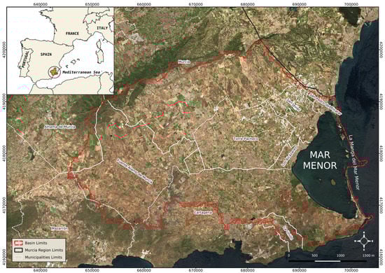
Figure 1.
Study area: Mar Menor Basin.
Despite the low rainfall, the soil features in the inland area of the basin, as well as its temperature and orography make the area very well fit for agricultural purposes. It has been cultivated since ancient times, and it has been progressively changing, during the last fifty years, from rain-fed to irrigated agriculture using water transferred from river Tagus, water from desalination plants and also underground water. The inland area of the basin is then one of the main agricultural surfaces in Murcia Region. According to regional statistics [51], rain-fed crops and low-density tree fields are currently less than 4500 ha, mainly cultivated with almond and olive trees. Some vineyard fields remain rain-fed, although they have been gradually abandoned and neglected, or have been transformed to use irrigation. Fields of irrigated grass crops alternate with irrigated dense tree crops in lower slope areas, representing nearly 38,000 ha. Main irrigated crops include perennials such as citrus and vineyards, and annual horticultural crops such as pepper, lettuce, artichoke, cauliflower, broccoli, melon and watermelon. Greenhouses cover more than 1500 ha in this area, although this figure only refers to surfaces completely closed with a plastic structure, leaving out any other type of cover such as nets used to prevent birds and insects from nibbling fruit on trees, and also to prevent hail damages.
Considering natural vegetation, there is a wide range of biodiversity and vegetation heterogeneity, mainly Mediterranean scrubs, although there are also patches of Mediterranean forest. The other main use in this territory is urban; many large urbanized surfaces, whose summer population increase is hard to quantify, can be found along the coastline delimiting the lagoon. The agricultural and residential development in the basin have been affecting the marine ecosystem for several decades [52,53].
2.2. Datasets
Eight SAR and MSI images (four images each) were selected. Instead of using a date for each season, imagery were selected according to the sowing and harvesting calendar for most of the crops in the area (Table 1). Including temporal reflectivity differences due to phenologic and agronomic stages increases the information available to discriminate among classes. Images were downloaded from Copernicus Open Access Hub repository [54].

Table 1.
Sentinel-1 and Sentinel-2 images used in this study.
2.2.1. Sentinel-2 Data
S2 Top of Atmosphere (TOA) data (L1C product) were acquired and corrected with ACOLITE [55,56,57] using the interface and code freely distributed by the Remote Sensing and Ecosystem Modeling (REMSEM) team, part of the Royal Belgian Institute of Natural Science (RBINS) and Operational Directorate Natural Environment (OD Nature). This correction method produced a more accurate classification than others such as Sen2Cor [58] or MAJA [59] in the same study area [60].
The MSI bands used were those with 10 and 20 m of spatial resolution (Table 2), with the latter resampled to 10 m resolution. Eleven bands per date are used, making a total of 44 features.
Table 2.
MSI spectral bands selected for classification, including Visible (VIS), Near Infra-Red (NIR) and Short Wave Infra-Red (SWIR).
The use of indices to recognize biophysical patterns on the Earth surface is a common and effective practice supported in a wide range of studies [61,62,63,64]. Indices highlight basic interactions between spectral variables. Hence, some indices were calculated from MSI bands:
- The Normalized Difference Vegetation Index (NDVI) [65] is used for measuring and monitoring vegetation cover and biomass production with satellite imagery. It is calculated with Equation (1).where is a narrow Near-Infrared (NIR) band for vegetation detection and is the red band (R) from S2A MSI.
- Tasseled cap brightness (TCB) [66] tries to emphasize spectral information from satellite imagery. Spectral bands from the visible and infrared (both near and shortwave) are used to obtain a matrix that highlights brightness, greenness, yellowness, nonesuch [66] and wetness [67] coefficients. In this case, we used the brightness equation, also known as the soil brightness index (SBI), which detects variations in soil reflectance. The equation for S2 is:where , and are the blue (B), green (G) and red (R) bands, respectively; is the NIR band; and and are the SWIR from S2A MSI.
- The Soil Adjusted Vegetation Index (SAVI) [68]: Due to the NDVI’s sensitivity to the proportion of soil and vegetation, this index is added to the NDVI a soil factor. In semiarid areas, this is a way to fit the index to background average reflectance. The equation is:where is the NIR band, is the R band and L is a factor for soil brightness with a value of 0.5 to fit with the majority of covers.
- The Normalized Difference Built-up Index (NDBI) [69] is used to distinguish built surfaces, which receive positive values, from bare soils. It is calculated with Equation (4):where is the SWIR band and the NIR band.
- The Modified Normalized Difference Water Index (MNDWI) [70] was proposed to detect superficial water. However, due to the relation between SWIR and wetness in soils, it can be also used to detect water in surfaces of vegetation or soil. The index is calculated with Equation (5):where is the G band and the SWIR band.
These indices were selected from the large amount of available indices because they cover the main features in the study area that affect reflectivity values and coverages (bare soil, vegetation and water availability). In addition, tasseled cup brightness averages reflectivity. There are five indices and four dates, making a total of 20 features.
Other metrics obtained from optical data are texture features, namely some of the Haralick’s GLCM texture metrics [3] based on tonal differences in pair of pixels within a predefined neighborhood. These metrics allow to distinguish vertical patterns of parallel lines more than one pixel wide. However, the large number of Haralick metrics and the use of four images multiply massively the number of possible layers. To tackle this problem we used only the three such metrics recommended in [71]: Contrast, entropy and angular second moment (Equations (6) to (8)).
where is the probability of i and j values occurring in adjacent pixels, and i and j are the labels of the column and row of the GLCM, respectively.
Such metrics were calculated on two summary layers per date: the first principal component of the spectral layers (that is, an albedo layer) and the NDVI. That means four dates, two summary layers and three GLCM metrics, making a total of 24 features.
2.2.2. Sentinel-1 Data
SAR images were selected in the Interferometric Wide (IW) mode with a full swath of 250 km and 5 × 20 m of spatial resolution in single look. This is the main acquisition mode over Earth’s surface using Terrain Observations by Progressive Scans SAR (TOPSAR), which provides three sub-swaths composed of a series of bursts, obtained by steering the beam from backward to forward in the azimuth direction with enough overlapping to ensure continuous coverage when merged. The incidence angle used for IW mode ranges from 29.1 to 46. To obtain the final Ground Range Detected (GRD) product, all bursts and sub-swath are merged and resampled to the common pixel spacing range, which means that GRD product data have been focused, multi-looked and projected to ground range using an Earth ellipsoid model.
Images taken in ascending or descending orbit may have differences in backscatter intensity because of the impact of the local incidence angle on the pixel area. All images used in this study are in descending mode with incidence angles ranging from almost 30.5 to slightly more than 46.4 degrees. The possible geometric issues were corrected applying a radiometric terrain correction in the preprocessing workflow [72], although the study area has little slope, so such geometric issues were probably not very serious before correcting them.
Pre-processing of S1 SAR images was carried out in SNAP 7.0 in batch mode, following the next steps: (1) radiometric calibration, (2) speckle filtering, (3) terrain correction and (4) conversion to dB. They were also resampled in step 3 to 10 m using the SRTM 1Sec HGT as Digital Elevation Model (DEM) with the nearest neighbor model. The projection used was the same used by the optical images to facilitate collocation with S2 data. Speckle filtering was performed with a Lee Sigma filter window size of 5 × 5, a sigma of 0.9 and a target size window of 3 × 3. S1 IW GRD images may include amplitude and intensity bands in co- and cross-polarization (VV, VH), but for this study only intensity was used.
In addition, DPSVI was calculated to separate bare soil from vegetation:
That means three features (VV, VH and DPSVI) per date, making a total of twelve features.
2.2.3. LiDAR Metrics
LiDAR is an active remote sensing system that uses laser pulses in the visible spectrum to record the altitude of several points on the Earth’s surface [73]. The Spanish Geographical Institute (IGN) maintains a National Aerial Orthophotography Plan (PNOA) [74] with a sampling density of 0.5 points per square meter. Data used in this study were obtained from August 2016 to March 2017. The recorded points are pre-classified according to the American Society for Photogrammetry and Remote Sensing (ASPRS) standards. Although the accuracy of this classification is unknown, we decided not to reclassify the points to avoid an over-complication of the process. This data can be downloaded from the website of the IGN’s National Centre for Geographic Information [75].
In the LiDAR preprocessing phase, points not belonging to bare soil, vegetation, buildings or water were filtered out. Then, the proportion of points of low vegetation (ppB), medium size vegetation (ppM), high vegetation (ppA), buildings (ppE) or water (ppH) were computed per each 10 × 10 m cell corresponding to the S2 images. Additionally, the number of medium or high vegetation points whose nearest neighbor is another medium or high vegetation point (Nvv) was also computed.
The altitude of the terrain obtained from the Spanish official DEM with resolution 5 m [76] was subtracted from each of the points to obtain their heights. With these estimated heights, we calculated the average height and standard deviation of each of the classes in each 10 × 10 cell. The resulting layers are average height of small vegetation (mZB), average height of medium size vegetation (mZM), average height of high vegetation (mZA), average height of building points (mZE), average height of ground points (mZG), standard deviation of small vegetation (sZB), standard deviation of medium size vegetation (sZM), standard deviation of high vegetation (sZA), standard deviation of building points (sZE) and standard deviation of ground points (sZG). If a cell has no points of a given class its average and standard deviation are estimated as 0.
The Hopkins statistic [77] is a method of measuring the cluster tendency of a dataset. It is defined as:
where is the distance of each point to its nearest neighbor, and is the distance in m of randomly chosen points to their nearest neighbor. The R package clustertend [78] allows to calculate the Hopkins index. We calculated the spatial cluster tendency (HI) of medium and high vegetation points in each 10 × 10 cell.
The NbClust function in the NbClust R package [79] allows to calculate the optimal number of clusters that might be extracted from a set of points. It provides 30 different cluster indices and selects the number of clusters that maximizes most of them. We also calculated the optimum number of clusters of medium and high vegetation points according to this function in each 10 × 10 cell (nCl).
Ripley’s K function [80] measures the tendency of points to appear dispersed or forming clusters. It is defined as:
where d is a given distance, A is the area of the analyzed territory, n is the number of points and is the number of points whose distance to point i is lower than d. Values of larger than the expected indicate a clustered point pattern, whereas values lower than the expected indicate a regular point pattern [80]. We calculated a relative K function as:
where is the expected value of assuming a random point distribution. As the function is calculated at several distances, it may be used to estimate the clustered/regular pattern at different scales. The R package spatstats [81] was used to calculate the K function.
We extracted four metrics from the function for medium and high vegetation points: the maximum and minimum values (wCv and wDv respectively) and the distances at which they occur (wCd and wDd respectively). In summary, twenty-two features from a single LiDAR image were obtained.
2.2.4. Training Datasets
Eleven different datasets were generated to obtain different classifications, five with each different predictor set separately: S1, S2, indices, texture and LiDAR metrics, and six other grouping different sets of predictors that added new information to every new dataset: S1+S2, S1+LiDAR, S2+LiDAR, S1+S2+LiDAR+indices, S1+S2+LiDAR+indices+ textures. The datasets by sensor or derived information included 44 reflectivity features from optical sensor data, 20 indices derived from them, 24 texture measures also obtained from optical data, 8 SAR bands and the 4 DPSVI derived from them, and 26 LiDAR metrics. Hence the number of features ranged from 12 (S1) to 126 (S1+S2+LiDAR+indices+texture). Table 3 summarizes all of the datasets. The names of the features are formed by combining the name of the layer and its date.
Table 3.
Summary of the datasets. The names of the features are formed by combining the name of the layer and its date.
2.3. Training Areas and Classification Scheme
Training areas were digitized using the aerial ortophotography from the Spanish PNOA [74] acquired in 2016 and 2019. A stratified sampling design was conducted to guarantee a reasonable presence of all classes. Representativity for the set was enhanced using Isolation Forest with the methodology proposed in [82], resulting in a total of 131 polygons, distributed as shown in Table 4. The classification scheme adopted was decided grouping land covers in the study area. Netting is a class related with recent agricultural practices that produces spectral responses different from those of greenhouses or irrigated crops. It consists of covering trees using nets with diverse mesh sizes to prevent both insects and birds from eating the fruit, and to protect from hail damages. Although some residual rain-fed areas exist in the study area, they are not included in the classification scheme because most of them are in a process of transformation to irrigation or being abandoned. In both cases their spectral signatures are similar to bare soil areas. We prefer to classify them as bare soil or scrub, as their surfaces are not in production any longer and are usually susceptible to a change of use.
Table 4.
Land covers taken into account in the classification, including the number of polygons for training and validation and number of total pixels per class.
2.4. Image Classification
Supervised pixel-based image classification was carried out with the different feature sets using three algorithms: RF, SVM and Multilayer Perceptron (MLP). Maximum Likelihood (MLC) was also used as a baseline classifier to compare these algorithms using the R package tabularMLC [83].
2.4.1. Random Forest
RF [84] is a non-parametric classification and regression method based on an ensemble of decision trees, usually between 500 and 2000, with two procedures to reduce correlation among trees: (1) each tree is trained with a bootstrapped subsample of the training data, and (2) the feature used to split each node of the trees is selected from a randomly generated subset of features. Although counterintuitive, this modifications reduce correlation among trees, giving more sense to the whole ensemble learning concept [8,85]. Once all trees are calibrated, each one contributes with a vote to classify every new pixel. Finally, the pixel is assigned to the most-voted class. Another option is to obtain the proportion of trees that voted for each class and use this information to obtain metrics of uncertainty.
The number of trees (ntree) and the number of features randomly chosen to split each node (mtry) are the parameters that the user must decide upon or optimize. The default values for the parameters ( and , where p is the number of features) usually allow a high accuracy to be reached [86]. In fact, depending on the problem, a smaller number of trees might be accurate enough, but 500 is a safe default that does not increase the computational cost excessively.
Although RF is not usually the most accurate machine learning (ML) method, it has several advantages [86,87,88,89,90,91]: (1) It is robust in case of high dimensionality, correlated features, small sample sizes or outliers. (2) It is possible to obtain a ranking of the importance of the features by measuring how the accuracy decreases when a feature is randomly reshuffled while the rest remains unchanged. (3) It is possible to evaluate the effect of the features in the model that can then be used as an explicative model, not only predictive. (4) It is possible to compute the distances between pairs of cases that could be used in an unsupervised classification. (5) It is computationally lighter than other ML methods, especially taking into account that it is not very sensitive to the values of the parameters, significantly reducing the computational cost of its calibration. (6) It provides an internal accuracy metric called Out-Of-Bag Cross Validation (OOB-CV) that has been considered an unbiased estimate of generalization error, provided that the training data are unbiased and randomly sampled. However, the authors of [90] highlighted that to calculate OOB-CV, RF internally splits each training polygon and uses its pixels both for training and testing. As pixels belonging to a single polygon are usually quite similar, the reported OOB-CV accuracy is easily overestimated. Ref. [90] proposed a modification of the algorithm (Spatial Dependence Random Forest—SDRF) to divide whole polygons, instead of pixels, into in-bag and out-of-bag.
The R libraries randomForest [92] and SDRF [90] (derived from the former) were used. The default value of mtry was used, but ntree was set as 2000 to avoid high variability in the feature importances when the number of predictors is quite high and they are collinear.
2.4.2. Support Vector Machines
SVM [93,94] is a very flexible classification algorithm that separates classes with optimal margin non-linear hyperplanes in the feature space. A cost parameter determines the degree of flexibility of such hyperplanes. Low flexibility could lead to underfitting, but high flexibility could lead to overfitting. A kernel transformation allows to linearize non-linear frontiers. Thus, the parameters used by SVM are the type of kernel, a parameter of the kernel function and the cost parameter. We used the R package kernlab [95].
SVM is very sensitive to the values of these parameters, so an optimization strategy is needed. In this case we used a Gaussian kernel whose parameter () controls the width of the function (low values tend to produce overfitting, and very high values tend to produce underfitting). This parameter was optimized following the strategy proposed in [96]. The C parameter was optimized using a five-fold cross-validation without repetition. Two cross-validation loops were designed to optimize parameter values in the inner loop and to test their accuracy in the outer loop.
2.4.3. Multilayer Perceptron
MLP is the most used variant of neural networks. It consists on an input layer, with as many inputs as predictors, one or mode hidden layers with a variable number of neurons, and an output layer with as many outputs as classes. Each neuron performs a linear combination of its inputs and applies a nonlinear transformation to the result to produce the output of the neuron. In this case we have used the sigmoid transformation function for the hidden layers and softmax for the output layer. The well-known backpropagation algorithm [97] is used to train the neural network. We used the RSNNS package [98] to build and calibrate the neural networks using the default learning rate and 100 epochs.
The optimization of the MLP was performed following the same strategy as in the case of SVM, optimizing the number of hidden layers (one or two) and the number of neurons (1 to 13).
2.5. Validation
Overal accuracy and kappa index were used for the comparison of the accuracy reached with different datasets, including 95% confidence intervals to decide the significance of differences. The validation used was a Leave-One-Out Cross-Validation (LOOCV) at the polygon level (n = 131); this process consists of iteratively training the classification models with all training polygons except one, which is left out of the process for testing. The caret library [99] was used to obtain confusion matrices and other accuracy statistics.
Both statistics have been subjected to recent critiques [100,101,102] as not giving all of the necessary information to evaluate the final map accuracy. However they have the advantage of providing a global statistics summarizing all of the accuracy issues, which is convenient when comparing large amounts of classifications; in addition, despite the criticism, both are still widely used.
However, when analyzing the final map, and according with the recommendations in the aforementioned papers, we will provide per-class accuracy statistics: precision recall and balanced accuracy and a graphical representation of omission and commission errors Surfaces obtained for each class will also be compared with official statistics to detect and explain any major deviation.
We calculated the 95% confidence interval of overall accuracy and kappa index, and considered that the estimated accuracies of two methods are different if their confidence intervals do not overlap.
2.6. Feature Selection
Because of the high number of features (126) and the high probability of multicollinearity among them, feature selection was advisable. The Variance Inflation Factor (VIF) is a feature selection method commonly used to detect collinear features. It was calculated for the predictors used in the best of the prior classifications. It estimates a linear model to predict each feature using the rest as predictors and computes its . The higher the VIF, the more collinear the feature. We calculated VIF in a recursive manner, eliminating in each step the feature with the highest VIF until all VIFs are smaller than a threshold. There are no rules of thumb to establish such as a threshold. Researchers in recent decades have suggested that this threshold should be established with caution, taking into account other factors that may have influence the variability of predictors [103,104]. We tested several thresholds and calculated the resulting OOB-CV accuracy using the SDRF function.
As VIF only takes into account collinearity, it might miss non-linear relations among features. Thus, once the appropriate VIF threshold was selected, the RF ranking of feature importance was used as a second feature selection step. Inside a leave-one-polygon-out CV loop, an RF model using 2000 trees was trained to obtain the feature importance ranking. The features were then sequentially eliminated from the least important until using just the most important. The resulting accuracies were then computed using SDRF. This process was repeated 131 times leaving out a different training polygon each time. The result was a list of 131 importance rankings and a matrix of accuracies with polygons in rows and features used in columns. Finally, the resulting rankings for all of the polygons were compared to check if they were similar enough to obtain a final feature subset with which to build an accurate and parsimonious classification model with RF.
3. Results
3.1. Classifications with Multisensor and Derived Predictors
Table 5 shows the classification accuracy metrics when using each of the datasets with the four classification algorithms as well as the tested combinations. Figure 2 shows overall accuracy values; it can be seen that the response of the three machine learning algorithms to the changes in predictor sets is very similar, whereas the response of MLC is clearly different.
Table 5.
Classification accuracy by dataset and classification method including overall accuracy and kappa index values with 95% confidence intervals. LOOCV by polygon (). The most accurate algorithm is highlighted in bold for each dataset combination.
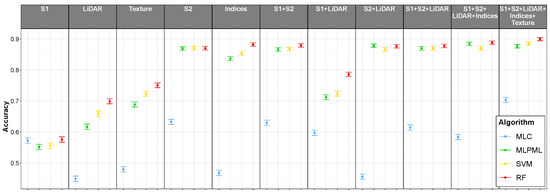
Figure 2.
Classification accuracy by dataset and classification method with 95% confidence intervals. LOOCV by polygon ().
It is noteworthy that, when using individual datasets, the greatest accuracy was reached using normalized indices. It seems that such indices are useful as a variable transformation to increase class separability. The accuracy of the different dataset combination was not higher, except when combining all datasets and all datasets except Texture. S1 and LiDAR alone produced quite less accurate models than S2- or S2-derived datasets, and even S1 and S2 did not outperform the S2 indices. It is only when all of the datasets were used in a synergetic way that maximum accuracy was achieved.
In most cases, RF was the most accurate method; only for S2 and S2+LiDAR, SVM and MLP, respectively, were the most accurate. However, in both cases RF cannot be considered significantly less accurate than those methods, as their confidence intervals overlap. In all cases the accuracy of the baseline model was significantly lower than that of the machine learning methods, except when using just S1 data. In this case Maximum Likelihood accuracy is not significantly lower than RF’s and both are significantly higher than SVM’s and MLP’s.
3.2. Feature Selection
As the highest accuracy is reached using all datasets and RF, the next step is to try to select the best subset of predictors to achieve a similar, or possibly better, accuracy. The first step is to use VIF to eliminate collinear predictors. Instead of choosing a fixed VIF threshold, several values were tested to calculate the resulting accuracy. Figure 3 shows the results corresponding to accuracy and kappa with the 95% confidence intervals. Although non-significantly higher accuracies were reached with larger thresholds, 160 was the finally used VIF threshold as it represents a step increase in accuracy with respect to smaller threshold values. The smaller the threshold, the smaller the number of features. This threshold means a reduction in the number of features from 126 to 84.
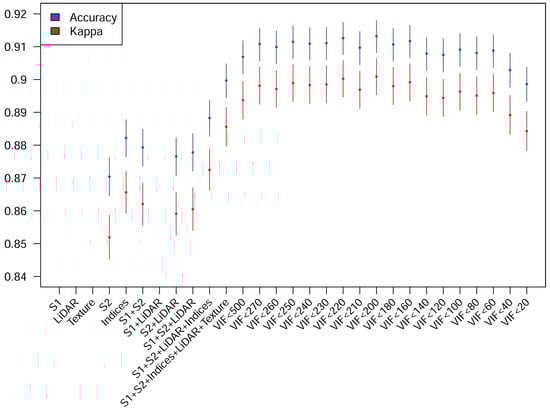
Figure 3.
Accuracy metrics and 95% confidence intervals achieved with every dataset and with the predictors selected increasing the VIF threshold. S1, Texture and S1+LiDAR results do not appear because they are lower than the y axis lower limit in the figure.
Figure 4 shows the per-polygon average accuracy and 95% confidence intervals when the least important features, starting with the 84 features selected by the VIF method, were removed. These means and confidence intervals were calculated from the 131 accuracy values calculated using SDRF OOB-CV using a different polygon for testing in each round. The final accuracy values were obtained from the validation of each individual polygon in the loop passage in which it was used as a test. According to these results, we decided to reject in each case the 21 least important features. As there were 131 different models, it was necessary to check if all of the models had the same important variables. A total of 59 features were present in all of the models, and just one was present in less than 50% of the models. Thus, we decided to reject this last feature and build a final classification model with the remaining features (Table 6). Interestingly, features from the five initial datasets remained as important after all of the feature selection process: S1 (8 out of 12 features), S2 (20 out of 44 features), indices (15 out of 20 features), texture (11 out of 24 features) and LiDAR (8 out of 26 features)—a total of 62 features.
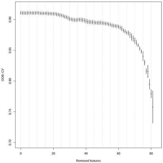
Figure 4.
Accuracy metrics achieved while decreasing the number of predictors.
Table 6.
Features selected for the final model. LiDAR features were derived from a single dataset recorded between August 2016 and March 2017.
3.3. Final Classification and Errors
The final classification using the selected features reached an accuracy of () and kappa of (). Omission and commission errors appear in Table 7 and, disaggregated, in Figure 5. Only the omission errors of scrub, impermeable areas, greenhouses and netting, and the commission errors of bare soil, greenhouses and netting exceeded 0.1, with both errors in netting beyond 0.2. Table 7 also includes omission and commission errors of the RF model using only S2 data and indices. The differences in natural surfaces are negligible, but all cultivated areas and bare soil show a substantial error reduction in the final model.
Table 7.
Omission and commission errors of the S1+S2 and the final classification.
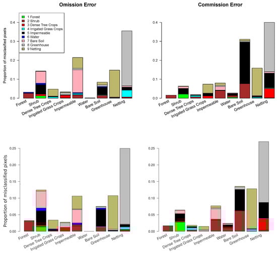
Figure 5.
Confusion between classes in the S2 model (above) and the final model (below).
Most of the confusions represent a really small proportion of pixels and can be considered residual noise. The most frequent confusions are between scrubs, bare soil and impermeable areas on the one hand, and greenhouses and netting on the other hand. We think these errors represent a more general lack of separability among classes. In semiarid areas, the distinction between scrubs and bare soil is very fuzzy. Moreover, in the surroundings of urban areas, there are frequently pixels mixing isolated houses, bare soil and some disperse scrubs. The confusion among greenhouses and netting is the quantitatively most salient (see also Table 8). It may be explained because the spectral signatures of both classes may be similar. However, it is not a very relevant confusion as both are, from an agronomic point of view, subclasses of irrigated crops.
Table 8.
Main classification statistics per class.
Figure 6 shows the importance ranking of the features included in the final model; features of all of the original datasets appear in the final model. The most important features included in the final model are reflectivities and normalized indices. The ten highest positions are occupied by optical features, with preference for spring dates: the four aerosol bands (B01), the spring green (B03), red edge (B06) and Infrared (B08) bands, and three indices, two from late spring and one of the early spring, NDVI and NDBI, and SAVI, respectively. In fact, the 23th first positions are occupied by reflectivity features or indices. The second dataset in terms of importance seems to be the SAR derived metrics, followed by LiDAR and texture.
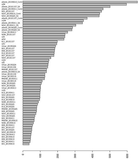
Figure 6.
Global feature importance.
Figure 7 shows the 20 most important features to classify each of the classes. S2 reflectivity and indices are the most important and predominant for all classes. In natural vegetation classes and greenhouses, only these variables appear. That is coherent with the lack of difference in omission and commission errors in natural covers shown in Table 7. SAR variables are important to distinguish water pixels, impermeable areas and irrigated grass crops. LiDAR variables appear in dense tree crops (mean height of buildings and high vegetation), irrigated grass crops (mean and standard deviation of medium vegetation height, and the distance of the minimum of the Ripley function for vegetation points) impermeable areas (mean height of buildings), bare soil (mean height of buildings and standard deviation of the height of ground points) and netting (mean and standard deviation of high vegetation points).
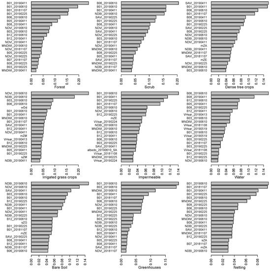
Figure 7.
Twenty most important features per class.
The predominance of S2 features reflects their well-known relevance in land cover classification. The new variables only add extra information related to the characteristics of some usually difficult to classify covers that allow for a better discrimination: height of the trees in tree crops and netting (that mostly cover tree crops), height and pattern of medium vegetation in grass crops, and height of buildings in impermeable (mostly urban) areas. The case of bare soil is more intriguing; the importance of the standard deviation of the height of ground points (with respect to the average of the pixel) may reflect erosive forms that are usual in semiarid environments; on the other hand, the average height of buildings is probably telling apart small constructions in bare soil areas from buildings in urban areas. In water pixels, SAR response is contributing to distinguish water from other dark covers.
3.4. Land Cover Maps
Figure 8 shows the estimated land cover maps using just S2 reflectivity and the final model after feature selection. There is a clear reduction in the impermeable and an increase in bare soil in irrigated crops. Table 9 shows the total extension for each class. According to the prior knowledge of the area, it seems to be quite qualitatively accurate. However, the surfaces assigned to Scrubs and Bare soils seem too high. The reason is, probably, that residual rain-fed crops have been classified as such. Discrimination between rain-fed and irrigated crops was discarded in this study due to the aforementioned issues (Section 2.1 and Section 2.5). Moreover, fallow fields remain, usually, uncultivated for two years, producing a spectral signature similar to classes where soil and sparse vegetation are dominant. Fields in very early stages of growing or that have been recently harvested show a similar issue. In this study these fields seem to have been labelled as bare soil, scrub or even as impermeable in some cases, as those shown in Figure 9. The number of image dates used seems to be not enough to avoid the problems of inter- or even intra-annual crop rotations; a larger date range might improve the results even more. We are aware that some rain-fed fields may remain, but it is a negligible amount and they are probably in the process of being abandoned or transformed into irrigated crops, due to the land use transformation dynamics in the study area.
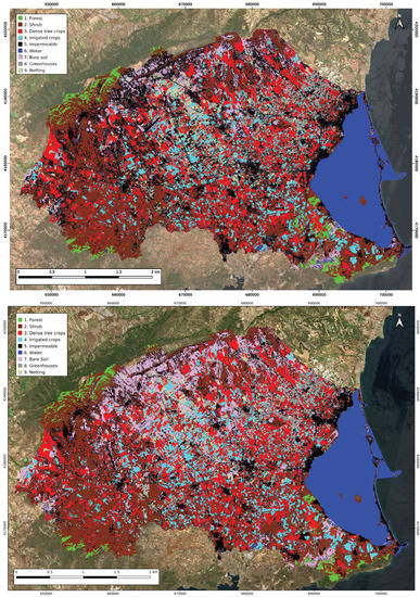
Figure 8.
Land cover map obtained with only S2 reflectivities (above) and with the final model (below).
Table 9.
Total surface classified for each class.
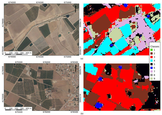
Figure 9.
Issues with fallow fields in classification: Right: (a) example of classification as bare soil (class 7); (b) example of classification as scrub (class 2). Left: both areas areas in ortho-photography (2019).
However, the process and methodology have demonstrated high accuracy at a regional scale, better than previous classifications made with data from only one sensor [60]. An example of the resulting map from both datasets appears in Figure 10. In this case the improvement in the classification accuracy when using data from several sensors is evident. Additionally, the delineation of the final polygons has been also improved.
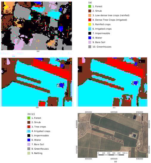
Figure 10.
Example of improvement in classification: (a) classification with S2 and indices in previous study [60]; (b) same area classified in the present study with S1 and S2; (c) same area classified in the present study with S1, S2 and LiDAR; (d) ortho-photography (2019).
4. Discussion
According to our results, adding S1 to S2 indices does not significantly increase classification accuracy. Chatziantoniou et al. [105] evaluated the combined use of S1 and S2 data for a regional-scale Mediterranean wetlands classification, reaching the same conclusion. In a study similar to ours, Denize et al. [6] achieved an overall accuracy of 0.81 with a kappa index of 0.77 using a multi-temporal study with images from winter autumn and spring to identify winter land uses in an area of study located in the north of France similar to Mar Menor basin in terms of field size and proximity to the coast. However, there are some important differences in climate, crop system and agricultural practices. Probably, the inclusion of features providing the height of the objects (LiDAR) and edges information (Texture) is the reason why the overall accuracy in this study is larger than in theirs.
Heinzel et al. [40] combined LiDAR features, some of the GLCM texture metrics (derived from color infrared images as well as from LiDAR) and optical features, achieving an overall accuracy, using all 464 features, of 0.88, but reducing the number of features to achieve at least 95% of accuracy, the model was reduced to only 14 features and its accuracy only decreased down to 0.85. Shingh et al. [106] used optical data and LiDAR, interpolating either point heights or intensities, to discriminate urban areas from vegetation covers, but without taking into account the point class information. They tested various resolutions and classification methods, reaching a maximum accuracy of 0.83 with 10 m resolution and 0.85 with 1 m resolution using maximum likelihood, and 0.79 and 0.82, respectively, using classification trees.
LiDAR-derived information has been successfully used to classify urban areas and different crops in small areas with high resolution [45,46]. Our classification schema is not as disaggregated and our study area is quite larger than in other studies. Hence, instead of fusing the LiDAR data with the reflectivity data using methods such as PCA or GLCM, we have extracted several metrics derived from LiDAR. After the feature selection process, only the most simple metrics (number of points in each 10x10 m pixel) remained in the dataset. Additionally, features from texture metrics helped in distinguishing vertical patterns of parallel lines more than one pixel wide, according to explanations of [71], so it may allow to recognize edge-like features inside a class.
Peña et al. [107] combined, among others, indices with textural features extracted from GLCM to classify between crops with different growing calendars, coming to the conclusion that the most influential features for an accurate classification were spectral indices, especially NDVI, distantly followed by texture features. Despite their secondary position in the importance ranking, texture features contributed to reduce uncertainty, mainly between different permanent crops, but the resulting overall accuracy was 0.80 with a kappa of 0.75. We have found similar accuracy using texture features, as some of these metrics remained as important after selection, although located in the tail of the importance ranking. Another similarity between both studies is the number of dates used, three and four, encompassing just a period of one year, although from different seasons: mid-spring and early and late summer in [107], and winter, early and late spring and autumn in ours.
In our study, just the addition of SAR data to reflectivity has not been enough to significantly increase the classification accuracy (Table 5), neither using optical data alone nor adding indices as well. Part of the problem may be the use of segmentation as a part of the process. Our study area is larger than in previous studies and the classes involved are more diverse, so it is difficult to obtain a segmentation parameter appropriate for all of the classes.
The usual threshold for the VIF analysis ranges from 5 to 10 [103,104]; however, in this case, it was necessary to raise the threshold to 160 in order to keep a high classification accuracy. This result highlights that very correlated features may still convey significant information for the classification process.
The most important features are the reflectivities, both globally and per class. However, the inclusion among the twenty most important features, for irrigated grass crops, impermeable surfaces and water, of SAR features, is interesting; water and urban areas have specific radar responses. On the other hand, LiDAR features appear in agricultural surfaces and bare soil. Height statistics of vegetation and ground points over a reference DEM seem to be the most relevant. There is also a clear relation between the class of vegetation recorded in the LiDAR points, and the estimated land cover.
It is noteworthy that the total surface classified as cultivated vegetation (Table 9) sums up more than expected according to the government official statistics [51]. The surface occupied by greenhouses also double the official amount. Adding all crop classes, we found almost 5000 ha more than in the official statistics. Previous remote sensing studies performed by [108], recently used as reference in a report about the state of the lagoon [109], already pointed out the existence of more irrigated surface than declared in regional statistics. Additionally, it has been reported [110] that the Hydrographic Demarcation of Segura River (DHS) is fighting against illegal irrigated areas, which are estimated to be over 7500 ha. If we take all of these facts into consideration, the extension estimated by our classification for cultivated vegetation seems realistic.
The main problem with the proposed methodology is the need to calculate all of the LiDAR metrics; it is a rather time-consuming process. Although the obtained accuracy increase is significant, at least with RF, it is true that it is not globally quantitatively important. However, it has been shown that some classes can indeed benefit from the extra information. Figure 10 shows a case in which the classification using only S2 is quite worse than using S1+S2 or S1+2+LiDAR. In this case the improvement in the classification accuracy when using data from several sensors is evident. Additionally, the delineation of the final polygons has also been improved.
On the other hand, RF has proven to be the most accurate model without any optimization, which saves computing time substantially. We acknowledge that the optimization carried out with SVM and MLP has not been as thorough as possible, especially taking into account that both methods are very sensitive to the values of their parameters. However, we think it is a fair comparison with RF, which has not been optimized at all. At any rate, the main objective of the work is to compare the accuracy achieved by different datasets, not by different algorithms.
5. Conclusions
Multi-sensor and multi-source predictors have been applied to land cover remote sensing classification in the Mar Menor basin. The use of all sources together showed significantly better accuracy results with respect to classifications made with just one source or diverse partial combinations of different datasets. To the best of our knowledge, such a combination of features has not been tested yet. It has demonstrated high efficacy in labelling this classification scheme at a regional scale.
The combination of all datasets produced a classification with an overall accuracy of almost 0.90 and a kappa index of more than 0.88, which were boosted to () and a kappa of () after feature selection. The removal of unnecessary features was successfully done by combining VIF, optimizing the collinearity threshold, and an analysis of importance of variables for every training and validation polygon of remaining features. The final number of features dropped from 126 to 62.
The balanced accuracies of all classes were higher than 0.9 and all errors of omission and commission were below 0.15 except in the netting class. This class is easily confounded with greenhouses; however, both are two different spectral classes of the same informational class—dense tree crops. Besides this confusion, a less important confusion case appeared among scrubs, bare soil and impermeable (urban) surfaces. The existence of fallow fields and intermixing of these three classes in periurban areas are the most probable causes of the problem, but further research must be conducted on the issue. Resulting land cover surfaces are coherent with other sources.
The analysis of per-class feature importance offers some insights about the relation among the new features and the classes that classification can help to increase.
Author Contributions
Conceptualization, C.V.-R. and F.A.-S.; methodology, C.V.-R. and F.A.-S.; software, F.A.-S. and F.G.-C.; validation, C.V.-R.; formal analysis, C.V.-R., F.G.-C. and F.A.-S.; investigation, C.V.-R.; resources, F.A.-S. and F.G.-C.; data curation, C.V.-R.; writing—original draft preparation, C.V.-R., F.G.-C. and F.A.-S.; writing—review and editing, C.V.-R., F.G.-C. and F.A.-S.; visualization, C.V.-R.; supervision, F.A.-S.; project administration, F.A.-S.; funding acquisition, F.A.-S. All authors have read and agreed to the published version of the manuscript.
Funding
This research was funded by the Spanish Ministry of Economy, Industry and Competitiveness/Agencia Estatal de Investigación/FEDER (Fondo Europeo de Desarrollo Regional) Grant Number CGL2017-84625-C2-2-R. C.V.R. is grateful for the financing of the pre-doctoral research by the Ministerio de Ciencia, Innovación y Universidades from the Government of Spain (FPU18/01447).
Data Availability Statement
The data that support the findings of this study are mostly available in the public domain: https://scihub.copernicus.eu/dhus/#/home (Sentinel images), accessed on 31 December 2022, https://centrodedescargas.cnig.es/CentroDescargas/index.jsp (LiDAR data), accessed on 31 December 2022. The training areas are openly available at https://doi.org/10.6084/m9.figshare.21231263.v1, accessed on 31 December 2022.
Conflicts of Interest
The authors declare no conflict of interest.
Abbreviations
The following abbreviations are used in this manuscript:
| ASPRS | American Society for Photogrammetry and Remote Sensing |
| DEM | Digital Elevation Model |
| DPSVI | Dual Polarization SAR Vegetation Index |
| ESA | European Spatial Agency |
| GLCM | Grey Level Coocurrence Matrix |
| GRD | Ground Range Detection |
| IW | Interferometric Wide |
| LiDAR | Light Detection and Ranging |
| LOO-CV | Leave One Out Cross Validation |
| ML | Machine Learning |
| MLC | Maximum Likelihood Classifier |
| MLP | Multilayer Perceptron |
| MNDWI | Modified Normalized Difference Water Index |
| MSI | MultiSpectral Instrument |
| mZB | average height of small vegetation |
| mZM | average height of medium size vegetation |
| mZA | average height of high vegetation |
| mZE | average height of building points |
| mZG | average height of ground points |
| NDBI | Normalized Difference Building Index |
| NDVI | Normalized Difference Vegetation Index |
| NIR | Near Infrared |
| Nvv | number of medium or high vegetation points whose nearest neighbor is a medium or high vegetation point |
| OD-Nature | Operational Directorate Natural Environment |
| OOB-CV | Out Of Bag Cross Validation |
| PNOA | National Aerial Orthophotography Plan |
| ppB | Proportion of points of low vegetation |
| ppM | Proportion of points of medium size vegetation |
| ppA | Proportion of points of high vegetation |
| ppE | Proportion of points of buildings |
| ppH | Proportion of points of water |
| REMSEM | Remote Sensing and Ecosystem Modelling |
| RBINS | Royal Belgian Institute of Natural Science |
| S1 | Sentinel 1 |
| S2 | Sentinel 2 |
| SAR | Synthetic Aperture Radar |
| SAVI | Soil Adjusted Vegetation Index |
| SBI | Soil Brightness Index |
| SVM | Support Vector Machine |
| SWIR | Short Wave Infrared |
| sZB | standard deviation of small vegetation height |
| sZM | standard deviation of medium size vegetation height |
| sZA | standard deviation of high vegetation |
| sZE | standard deviation of building points |
| sZG | standard deviation of ground points |
| TCB | Tasselled Cap Brightness |
| TOA | Top Of the Atmosphere |
| TOPSAR | Terrain Observation by Progresssive Scans SAR |
| VIF | Variance Inflation Factor |
| wCv | Maximum value of the Ripley’s K function |
| wDv | Minimum value of the Ripley’s K function |
| wCd | Distance of the maximum value of the Ripley’s K function |
| wDd | Distance of the minimum value of the Ripley’s K function |
References
- Berberoglu, S.; Curran, P.J.; Lloyd, C.D.; Atkinson, P.M. Texture classification of Mediterranean land cover. Int. J. Appl. Earth Obs. Geoinf. 2007, 9, 322–334. [Google Scholar] [CrossRef]
- Ezzine, H.; Bouziane, A.; Ouazar, D. Seasonal comparisons of meteorological and agricultural drought indices in Morocco using open short time-series data. Int. J. Appl. Earth Obs. Geoinf. 2014, 26, 36–48. [Google Scholar] [CrossRef]
- Haralick, R.M. Statistical and structural approaches to texture. Proc. IEEE 1979, 67, 786–804. [Google Scholar] [CrossRef]
- Zhou, P.; Han, J.; Cheng, G.; Zhang, B. Learning compact and discriminative stacked autoencoder for hyperspectral image classification. IEEE Trans. Geosci. Remote Sens. 2019, 57, 4823–4833. [Google Scholar] [CrossRef]
- Kupidura, P. The comparison of different methods of texture analysis for their efficacy for land use classification in satellite imagery. Remote Sens. 2019, 11, 1233. [Google Scholar] [CrossRef]
- Denize, J.; Hubert-Moy, L.; Betbeder, J.; Corgne, S.; Baudry, J.; Pottier, E. Evaluation of using sentinel-1 and-2 time-series to identify winter land use in agricultural landscapes. Remote Sens. 2019, 11, 37. [Google Scholar] [CrossRef]
- Campos-Taberner, M.; García-Haro, F.J.; Martínez, B.; Sánchez-Ruíz, S.; Gilabert, M.A. A Copernicus Sentinel-1 and Sentinel-2 classification framework for the 2020+ European common agricultural policy: A case study in València (Spain). Agronomy 2019, 9, 556. [Google Scholar] [CrossRef]
- Gomariz-Castillo, F.; Alonso-Sarría, F.; Cánovas-García, F. Improving classification accuracy of multi-temporal landsat images by assessing the use of different algorithms, textural and ancillary information for a mediterranean semiarid area from 2000 to 2015. Remote Sens. 2017, 9, 1058. [Google Scholar] [CrossRef]
- Zhang, W.; Brandt, M.; Wang, Q.; Prishchepov, A.V.; Tucker, C.J.; Li, Y.; Lyu, H.; Fensholt, R. From woody cover to woody canopies: How Sentinel-1 and Sentinel-2 data advance the mapping of woody plants in savannas. Remote Sens. Environ. 2019, 234, 111465. [Google Scholar] [CrossRef]
- Mandal, D.; Kumar, V.; Bhattacharya, A.; Rao, Y.S.; Siqueira, P.; Bera, S. Sen4Rice: A processing chain for differentiating early and late transplanted rice using time-series Sentinel-1 SAR data with Google Earth engine. IEEE Geosci. Remote Sens. Lett. 2018, 15, 1947–1951. [Google Scholar] [CrossRef]
- Arias, M.; Campo-Bescós, M.Á.; Álvarez-Mozos, J. Crop Classification Based on Temporal Signatures of Sentinel-1 Observations over Navarre Province, Spain. Remote Sens. 2020, 12, 278. [Google Scholar] [CrossRef]
- Mandal, D.; Kumar, V.; Ratha, D.; Dey, S.; Bhattacharya, A.; Lopez-Sanchez, J.M.; McNairn, H.; Rao, Y.S. Dual polarimetric radar vegetation index for crop growth monitoring using sentinel-1 SAR data. Remote Sens. Environ. 2020, 247, 111954. [Google Scholar] [CrossRef]
- Inglada, J.; Vincent, A.; Arias, M.; Marais-Sicre, C. Improved early crop type identification by joint use of high temporal resolution SAR and optical image time series. Remote Sens. 2016, 8, 362. [Google Scholar] [CrossRef]
- Veloso, A.; Mermoz, S.; Bouvet, A.; Le Toan, T.; Planells, M.; Dejoux, J.F.; Ceschia, E. Understanding the temporal behavior of crops using Sentinel-1 and Sentinel-2-like data for agricultural applications. Remote Sens. Environ. 2017, 199, 415–426. [Google Scholar] [CrossRef]
- Periasamy, S. Significance of dual polarimetric synthetic aperture radar in biomass retrieval: An attempt on Sentinel-1. Remote Sens. Environ. 2018, 217, 537–549. [Google Scholar] [CrossRef]
- Kumar, P.; Prasad, R.; Gupta, D.; Mishra, V.; Vishwakarma, A.; Yadav, V.; Bala, R.; Choudhary, A.; Avtar, R. Estimation of winter wheat crop growth parameters using time series Sentinel-1A SAR data. Geocarto Int. 2018, 33, 942–956. [Google Scholar] [CrossRef]
- Vreugdenhil, M.; Wagner, W.; Bauer-Marschallinger, B.; Pfeil, I.; Teubner, I.; Rüdiger, C.; Strauss, P. Sensitivity of Sentinel-1 backscatter to vegetation dynamics: An Austrian case study. Remote Sens. 2018, 10, 1396. [Google Scholar] [CrossRef]
- Topaloğlu, R.H.; Sertel, E.; Musaoğlu, N. Assessment of Classification Accuracies of SENTINEL-2 and LANDSAT-8 Data for Land Cover/Use Mapping. Int. Arch. Photogramm. Remote Sens. Spatial Inf. Sci. 2016, XLI-B8, 1055–1059. [Google Scholar] [CrossRef]
- Borrás, J.; Delegido, J.; Pezzola, A.; Pereira, M.; Morassi, G.; Camps-Valls, G. Clasificación de usos del suelo a partir de imágenes Sentinel-2. Rev. De Teledetección 2017, 48, 55–66. [Google Scholar] [CrossRef]
- Thanh Noi, P.; Kappas, M. Comparison of random forest, k-nearest neighbor, and support vector machine classifiers for land cover classification using Sentinel-2 imagery. Sensors 2018, 18, 18. [Google Scholar] [CrossRef]
- Drusch, M.; Del Bello, U.; Carlier, S.; Colin, O.; Fernandez, V.; Gascon, F.; Hoersch, B.; Isola, C.; Laberinti, P.; Martimort, P.; et al. Sentinel-2: ESA’s optical high-resolution mission for GMES operational services. Remote Sens. Environ. 2012, 120, 25–36. [Google Scholar] [CrossRef]
- Brinkhoff, J.; Vardanega, J.; Robson, A.J. Land cover classification of nine perennial crops using sentinel-1 and-2 data. Remote Sens. 2020, 12, 96. [Google Scholar] [CrossRef]
- Haas, J.; Ban, Y. Sentinel-1A SAR and sentinel-2A MSI data fusion for urban ecosystem service mapping. Remote Sens. Appl. Soc. Environ. 2017, 8, 41–53. [Google Scholar] [CrossRef]
- Tavares, P.A.; Beltrão, N.E.S.; Guimarães, U.S.; Teodoro, A.C. Integration of sentinel-1 and sentinel-2 for classification and LULC mapping in the urban area of Belém, eastern Brazilian Amazon. Sensors 2019, 19, 1140. [Google Scholar] [CrossRef] [PubMed]
- Amoakoh, A.O.; Aplin, P.; Awuah, K.T.; Delgado-Fernandez, I.; Moses, C.; Alonso, C.P.; Kankam, S.; Mensah, J.C. Testing the Contribution of Multi-Source Remote Sensing Features for Random Forest Classification of the Greater Amanzule Tropical Peatland. Sensors 2021, 21, 3399. [Google Scholar] [CrossRef] [PubMed]
- Masiza, W.; Chirima, J.G.; Hamandawana, H.; Pillay, R. Enhanced mapping of a smallholder crop farming landscape through image fusion and model stacking. Int. J. Remote. Sens. 2020, 41, 8736–8753. [Google Scholar] [CrossRef]
- Dobrinić, D.; Medak, D.; Gašparović, M. Integration of multitemporal Sentinel-1 and Sentinel-2 imagery for land-cover classification using machine learning methods. Int. Arch. Photogramm. Remote. Sens. Spat. Inf. Sci. 2020, XLIII-B1-2, 91–98. [Google Scholar] [CrossRef]
- De Luca, G.; MN Silva, J.; Di Fazio, S.; Modica, G. Integrated use of Sentinel-1 and Sentinel-2 data and open-source machine learning algorithms for land cover mapping in a Mediterranean region. Eur. J. Remote Sens. 2022, 55, 52–70. [Google Scholar] [CrossRef]
- De Fioravante, P.; Luti, T.; Cavalli, A.; Giuliani, C.; Dichicco, P.; Marchetti, M.; Chirici, G.; Congedo, L.; Munafò, M. Multispectral Sentinel-2 and SAR Sentinel-1 Integration for Automatic Land Cover Classification. Land 2021, 10, 611. [Google Scholar] [CrossRef]
- Kleeschulte, S.; Banko, G.; Smith, G.; Arnold, S.; Scholz, J.; Kosztra, B.; Maucha, G. Technical Specifications for Implementation of a New Land-Monitoring Concept Based on EAGLE, D5: Design Concept and CLC+ Backbone, Technical Specifications, CLC+ Core and CLC+ Instances Draft Specifications, Including Requirements Review; Technical Report; European Environment Agency: Copenhagen, Denmark, 2020. [Google Scholar]
- Wang, Y.; Liu, H.; Sang, L.; Wang, J. Characterizing Forest Cover and Landscape Pattern Using Multi-Source Remote Sensing Data with Ensemble Learning. Remote Sens. 2022, 14, 5470. [Google Scholar] [CrossRef]
- Han, Y.; Guo, J.; Ma, Z.; Wang, J.; Zhou, R.; Zhang, Y.; Hong, Z.; Pan, H. Habitat Prediction of Northwest Pacific Saury Based on Multi-Source Heterogeneous Remote Sensing Data Fusion. Remote Sens. 2022, 14, 5061. [Google Scholar] [CrossRef]
- Marais-Sicre, C.; Fieuzal, R.; Baup, F. Contribution of multispectral (optical and radar) satellite images to the classification of agricultural surfaces. Int. J. Appl. Earth Obs. Geoinf. 2020, 84, 101972. [Google Scholar] [CrossRef]
- Wuyun, D.; Sun, L.; Sun, Z.; Chen, Z.; Hou, A.; Teixeira Crusiol, L.G.; Reymondin, L.; Chen, R.; Zhao, H. Mapping fallow fields using Sentinel-1 and Sentinel-2 archives over farming-pastoral ecotone of Northern China with Google Earth Engine. Giscience Remote. Sens. 2022, 59, 333–353. [Google Scholar] [CrossRef]
- Berger, K.; Machwitz, M.; Kycko, M.; Kefauver, S.C.; Van Wittenberghe, S.; Gerhards, M.; Verrelst, J.; Atzberger, C.; Tol, C.v.d.; Damm, A.; et al. Multi-sensor spectral synergies for crop stress detection and monitoring in the optical domain: A review. Remote. Sens. Environ. 2022, 280, 113198. [Google Scholar] [CrossRef] [PubMed]
- Andalibi, L.; Ghorbani, A.; Darvishzadeh, R.; Moameri, M.; Hazbavi, Z.; Jafari, R.; Dadjou, F. Multisensor Assessment of Leaf Area Index across Ecoregions of Ardabil Province, Northwestern Iran. Remote Sens. 2022, 14, 5731. [Google Scholar] [CrossRef]
- Zhang, N.; Chen, M.; Yang, F.; Yang, C.; Yang, P.; Gao, Y.; Shang, Y.; Peng, D. Forest Height Mapping Using Feature Selection and Machine Learning by Integrating Multi-Source Satellite Data in Baoding City, North China. Remote Sens. 2022, 14, 4434. [Google Scholar] [CrossRef]
- Guerra-Hernandez, J.; Narine, L.L.; Pascual, A.; Gonzalez-Ferreiro, E.; Botequim, B.; Malambo, L.; Neuenschwander, A.; Popescu, S.C.; Godinho, S. Aboveground biomass mapping by integrating ICESat-2, SENTINEL-1, SENTINEL-2, ALOS2/PALSAR2, and topographic information in Mediterranean forests. Giscience Remote. Sens. 2022, 59, 1509–1533. [Google Scholar] [CrossRef]
- Kabisch, N.; Selsam, P.; Kirsten, T.; Lausch, A.; Bumberger, J. A multi-sensor and multi-temporal remote sensing approach to detect land cover change dynamics in heterogeneous urban landscapes. Ecol. Indic. 2019, 99, 273–282. [Google Scholar] [CrossRef]
- Heinzel, J.; Koch, B. Investigating multiple data sources for tree species classification in temperate forest and use for single tree delineation. Int. J. Appl. Earth Obs. Geoinf. 2012, 18, 101–110. [Google Scholar] [CrossRef]
- Montesano, P.; Cook, B.; Sun, G.; Simard, M.; Nelson, R.; Ranson, K.; Zhang, Z.; Luthcke, S. Achieving accuracy requirements for forest biomass mapping: A spaceborne data fusion method for estimating forest biomass and LiDAR sampling error. Remote Sens. Environ. 2013, 130, 153–170. [Google Scholar] [CrossRef]
- Chen, L.; Ren, C.; Bao, G.; Zhang, B.; Wang, Z.; Liu, M.; Man, W.; Liu, J. Improved Object-Based Estimation of Forest Aboveground Biomass by Integrating LiDAR Data from GEDI and ICESat-2 with Multi-Sensor Images in a Heterogeneous Mountainous Region. Remote. Sens. 2022, 14, 2743. [Google Scholar] [CrossRef]
- Morin, D.; Planells, M.; Baghdadi, N.; Bouvet, A.; Fayad, I.; Le Toan, T.; Mermoz, S.; Villard, L. Improving Heterogeneous Forest Height Maps by Integrating GEDI-Based Forest Height Information in a Multi-Sensor Mapping Process. Remote. Sens. 2022, 14, 2079. [Google Scholar] [CrossRef]
- Torres de Almeida, C.; Gerente, J.; Rodrigo dos Prazeres Campos, J.; Caruso Gomes Junior, F.; Providelo, L.; Marchiori, G.; Chen, X. Canopy Height Mapping by Sentinel 1 and 2 Satellite Images, Airborne LiDAR Data, and Machine Learning. Remote Sens. 2022, 14, 4112. [Google Scholar] [CrossRef]
- Zhong, Y.; Cao, Q.; Zhao, J.; Ma, A.; Zhao, B.; Zhang, L. Optimal decision fusion for urban land-use/land-cover classification based on adaptive differential evolution using hyperspectral and LiDAR data. Remote Sens. 2017, 9, 868. [Google Scholar] [CrossRef]
- Feng, Q.; Zhu, D.; Yang, J.; Li, B. Multisource hyperspectral and LiDAR data fusion for urban land-use mapping based on a modified two-branch convolutional neural network. ISPRS Int. J. Geo-Inf. 2019, 8, 28. [Google Scholar] [CrossRef]
- Rittenhouse, C.; Berlin, E.; Mikle, N.; Qiu, S.; Riordan, D.; Zhu, Z. An Object-Based Approach to Map Young Forest and Shrubland Vegetation Based on Multi-Source Remote Sensing Data. Remote Sens. 2022, 14, 1091. [Google Scholar] [CrossRef]
- Ali, A.; Abouelghar, M.; Belal, A.; Saleh, N.; Yones, M.; Selim, A.; Amin, M.; Elwesemy, A.; Kucher, D.; Maginan, S.; et al. Crop Yield Prediction Using Multi Sensors Remote Sensing (Review Article). Egypt. J. Remote Sens. Space Sci. 2022, 25, 711–716. [Google Scholar] [CrossRef]
- Orynbaikyzy, A.; Gessner, U.; Mack, B.; Conrad, C. Crop Type Classification Using Fusion of Sentinel-1 and Sentinel-2 Data: Assessing the Impact of Feature Selection, Optical Data Availability, and Parcel Sizes on the Accuracies. Remote. Sens. 2020, 12, 2779. [Google Scholar] [CrossRef]
- Wu, F.; Ren, Y.; Wang, X. Application of Multi-Source Data for Mapping Plantation Based on Random Forest Algorithm in North China. Remote Sens. 2022, 14, 4946. [Google Scholar] [CrossRef]
- CARM. Estadística Agraria Regional. 2021. Available online: https://www.carm.es/web/pagina?IDCONTENIDO=1174&RASTRO=c1415$m&IDTIPO=100 (accessed on 15 April 2021).
- Martínez, J.; Esteve, M.; Martínez-Paz, J.; Carreño, F.; Robledano, F.; Ruiz, M.; Alonso-Sarría, F. Simulating management options and scenarios to control nutrient load to Mar Menor, Southeast Spain. Transitional Waters Monogr. 2007, 1, 53–70. [Google Scholar] [CrossRef]
- Giménez-Casalduero, F.; Gomariz-Castillo, F.; Alonso-Sarria, F.; Cortés, E.; Izquierdo-Muñoz, A.; Ramos-Esplá, A. Pinna nobilis in the Mar Menor coastal lagoon: A story of colonization and uncertainty. Mar. Ecol. Prog. Ser. 2020, 652, 77–94. [Google Scholar] [CrossRef]
- European Commission. Copernicus Open Access Hub. 2021. Available online: https://scihub.copernicus.eu/ (accessed on 15 April 2021).
- Vanhellemont, Q.; Ruddick, K. Acolite for Sentinel-2: Aquatic applications of MSI imagery. In Proceedings of the 2016 ESA Living Planet Symposium, Prague, Czech Republic, 9–13 May 2016; pp. 9–13. [Google Scholar]
- Vanhellemont, Q.; Ruddick, K. Atmospheric correction of metre-scale optical satellite data for inland and coastal water applications. Remote Sens. Environ. 2018, 216, 586–597. [Google Scholar] [CrossRef]
- Vanhellemont, Q. Adaptation of the dark spectrum fitting atmospheric correction for aquatic applications of the Landsat and Sentinel-2 archives. Remote Sens. Environ. 2019, 225, 175–192. [Google Scholar] [CrossRef]
- Main-Knorn, M.; Pflug, B.; Louis, J.; Debaecker, V.; Müller-Wilm, U.; Gascon, F. Sen2Cor for Sentinel-2. In Proceedings of the Image and Signal Processing for Remote Sensing XXIII; Bruzzone, L., Ed.; SPIE: Warsaw, Poland, 2017. [Google Scholar] [CrossRef]
- Lonjou, V.; Desjardins, C.; Hagolle, O.; Petrucci, B.; Tremas, T.; Dejus, M.; Makarau, A.; Auer, S. MACCS-ATCOR joint algorithm (MAJA). In Proceedings of the Remote Sensing of Clouds and the Atmosphere XXI, Edinburgh, UK, 28–29 September 2016; Comerón, A., Kassianov, E.I., Schäfer, K., Eds.; International Society for Optics and Photonics, SPIE: Bellingham, WA, USA, 2016; Volume 10001, pp. 25–37. [Google Scholar] [CrossRef]
- Valdivieso-Ros, M.; Alonso-Sarria, F.; Gomariz-Castillo, F. Effect of Different Atmospheric Correction Algorithms on Sentinel-2 Imagery Classification Accuracy in a Semiarid Mediterranean Area. Remote Sens. 2021, 13, 1770. [Google Scholar] [CrossRef]
- Klein, I.; Gessner, U.; Dietz, A.J.; Kuenzer, C. Global WaterPack–A 250 m resolution dataset revealing the daily dynamics of global inland water bodies. Remote Sens. Environ. 2017, 198, 345–362. [Google Scholar] [CrossRef]
- Mostafiz, C.; Chang, N.B. Tasseled cap transformation for assessing hurricane landfall impact on a coastal watershed. Int. J. Appl. Earth Obs. Geoinf. 2018, 73, 736–745. [Google Scholar] [CrossRef]
- Yang, X.; Qin, Q.; Grussenmeyer, P.; Koehl, M. Urban surface water body detection with suppressed built-up noise based on water indices from Sentinel-2 MSI imagery. Remote Sens. Environ. 2018, 219, 259–270. [Google Scholar] [CrossRef]
- Hong, C.; Jin, X.; Ren, J.; Gu, Z.; Zhou, Y. Satellite data indicates multidimensional variation of agricultural production in land consolidation area. Sci. Total Environ. 2019, 653, 735–747. [Google Scholar] [CrossRef]
- Rouse, J.; Haas, R.; Schell, J.; Deering, D. Monitoring the vernal advancement and retrogradation (green wave effect) of natural vegetation. Prog. Rep. RSC 1978-1. Remote Sens. Center Tex. A&M Univ. Coll. Stn. 1973, 93. [Google Scholar]
- Kauth, R.J.; Thomas, G.S. The Tasselled-Cap—A Graphic Description of the Spectral-Temporal Development of Agricultural Crops as Seen by Landsat. In Proceedings of the Symposium on Machine Processing of Remotely Sensed Data, West Lafayette, IN, USA, 29 June–1 July 1976; Purdue University: West Lafayette, IN, USA, 1976; pp. 41–51. [Google Scholar]
- Crist, E.P. A TM tasseled cap equivalent transformation for reflectance factor data. Remote Sens. Environ. 1985, 17, 301–306. [Google Scholar] [CrossRef]
- Huete, A.R. A soil-adjusted vegetation index (SAVI). Remote Sens. Environ. 1988, 25, 295–309. [Google Scholar] [CrossRef]
- Chen, X.L.; Zhao, H.M.; Li, P.X.; Yin, Z.Y. Remote sensing image-based analysis of the relationship between urban heat island and land use/cover changes. Remote Sens. Environ. 2006, 104, 133–146. [Google Scholar] [CrossRef]
- Xu, H. Modification of normalized difference water index (NDWI) to enhanced open water features in remotely sensed imagery. Int. J. Remote Sens. 2006, 27, 3025–3033. [Google Scholar] [CrossRef]
- Hall-Beyer, M. Practical guidelines for choosing GLCM textures to use in landscape classification tasks over a range of moderate spatial scales. Int. J. Remote Sens. 2017, 38, 1312–1338. [Google Scholar] [CrossRef]
- Filipponi, F. Sentinel-1 GRD preprocessing workflow. Multidiscip. Digit. Publ. Inst. Proc. 2019, 18, 11. [Google Scholar]
- Dong, P.; Chen, Q. LiDAR Remote Sensing and Applications; CRC Press Taylor & Francis Group: Boca Raton, FL, USA, 2018; p. 200. [Google Scholar] [CrossRef]
- IGN. Plan Nacional de Ortofotografía. 2019. Available online: https://pnoa.ign.es/ (accessed on 15 April 2021).
- IGN. Centro de Descargas del Centro Nacional de Información Geográfica. 2021. Available online: https://centrodedescargas.cnig.es/CentroDescargas/index.jsp (accessed on 2 November 2022).
- IGN. Modelo Digital del Terreno Con Paso de Malla de 5 m. 2020. Available online: https://centrodedescargas.cnig.es/CentroDescargas/documentos/MDT05_recursos.zip (accessed on 1 February 2021).
- Hopkins, B.; Skellam, J. A new method for determining the type of distribution of plant individuals. Ann. Bot. 1954, 18, 213–227. [Google Scholar] [CrossRef]
- YiLan, L.; RuTong, Z. Clustertend: Check the Clustering Tendency; R Package Version 1.4. 2015. Available online: https://cran.r-project.org/web/packages/clustertend/ (accessed on 31 December 2021).
- Charrad, M.; Ghazzali, N.; Boiteau, V.; Niknafs, A. NbClust: An R package for Determining the Relevant Number of Clusters in a Data Set. J. Stat. Softw. 2014, 61, 36. [Google Scholar] [CrossRef]
- Lloyd, C. Spatial Data Analysis: An Introduction for GIS Users; Oxford University Press: Oxford, UK, 2010; p. 206. [Google Scholar]
- Baddeley, A.; Rubak, E.; Turner, R. Spatial Point Patterns: Methodology and Applications with R; Chapman and Hall/CRC Press: London, UK, 2015; p. 810. [Google Scholar] [CrossRef]
- Alonso-Sarria, F.; Valdivieso-Ros, C.; Gomariz-Castillo, F. Isolation Forests to Evaluate Class Separability and the Representativeness of Training and Validation Areas in Land Cover Classification. Remote Sens. 2019, 11, 3000. [Google Scholar] [CrossRef]
- Hamamura, C. tabularMLC: Tabular Maximum Likelihood Classifier; R Package Version 0.0.3; 2021. Available online: https://cran.r-project.org/web/packages/tabularMLC/ (accessed on 31 December 2021).
- Breiman, L. Random Forests. Mach. Learn. 2001, 45, 5–32. [Google Scholar] [CrossRef]
- James, G.; Witten, D.; Hastie, T.; Tibshirani, R. An Introduction to Statistical Learning; Springer Texts in Statistics; Springer New York: New York, NY, USA, 2013; Volume 103, p. 426. [Google Scholar] [CrossRef]
- Liaw, A.; Wiener, M. The randomforest package. R News 2002, 2, 18–22. [Google Scholar]
- Ghimire, B.; Rogan, J.; Rodríguez-Galiano, V.; Panday, P.; Neeti, N. An Evaluation of Bagging, Boosting, and Random Forests for Land-Cover Classification in Cape Cod, Massachusetts, USA. GIScience Remote Sens. 2012, 49, 623–643. [Google Scholar] [CrossRef]
- Rodríguez-Galiano, V.; Ghimire, B.; Rogan, J.; Chica-Olmo, M.; Rigol-Sanchez, J. An Assessment of the Effectiveness of a Random Forest Classifier for Land-Cover Classification. ISPRS J. Photogramm. Remote Sens. 2012, 67, 93–104. [Google Scholar] [CrossRef]
- Belgiu, M.; Drăgut, L. Random forest in remote sensing: A review of applications and future directions. ISPRS J. Photogramm. Remote Sens. 2016, 114, 24–31. [Google Scholar] [CrossRef]
- Cánovas-García, F.; Alonso-Sarría, F.; Gomariz-Castillo, F.; Oñate-Valdivieso, F. Modification of the random forest algorithm to avoid statistical dependence problems when classifying remote sensing imagery. Comput. Geosci. 2017, 103, 1–11. [Google Scholar] [CrossRef]
- Maxwell, A.; Warner, T.; Fang, F. Implementation of machine-learning classification in remote sensing: An applied review. Int. J. Remote Sens. 2018, 39, 2784–2817. [Google Scholar] [CrossRef]
- Liaw, A.; Wiener, M. Classification and Regression by randomForest. R News 2002, 2, 18–22. [Google Scholar]
- Camps-Valls, G.; Bruzzone, L.E. Kernel Methods for Remote Sensing Data Analysis; John Wiley & Sons, Ltd.: Chichester, UK, 2009. [Google Scholar]
- Mountrakis, G.; Im, J.; Ogole, C. Support vector machines in remote sensing: A review. ISPRS J. Photogramm. Remote Sens. 2011, 66, 247–259. [Google Scholar] [CrossRef]
- Karatzoglou, A.; Smola, A.; Hornik, K.; Zeileis, A. kernlab—An S4 Package for Kernel Methods in R. J. Stat. Softw. 2004, 11, 1–20. [Google Scholar] [CrossRef]
- Caputo, B.; Sim, K.; Furesjo, F.; Smola, A. Appearance–Based Object Recognition Using SVMs: Which Kernel Should I Use? In Proceedings of the NIPS Workshop on Statistical Methods for Computational Experiments in Visual Processing and Computer Vision; dos Santos, E.M., Gomes, H.M., Eds.; IEEE Computer Society: Los Alamitos, CA, USA, 2002. [Google Scholar]
- Kuhn, M.; Johnson, K. Applied Predictive Modeling; Springer: Berlin/Heidelberg, Germany, 2013. [Google Scholar]
- Bergmeir, C.; Benítez, J.M. Neural Networks in R Using the Stuttgart Neural Network Simulator: RSNNS. J. Stat. Softw. 2012, 46, 1–26. [Google Scholar] [CrossRef]
- Kuhn, M. Caret: Classification and Regression Training; R Package Version 6.0-93. 2022. Available online: https://cran.r-project.org/web/packages/caret/ (accessed on 31 December 2022).
- Stehman, S.V.; Foody, G.M. Key issues in rigorous accuracy assessment of land cover products. Remote Sens. Environ. 2019, 231, 111199. [Google Scholar] [CrossRef]
- Foody, G. Explaining the unsuitability of the kappa coefficient in the assessment and comparison of the accuracy of thematic maps obtained by image classification. Remote Sens. Environ. 2020, 239, 111630. [Google Scholar] [CrossRef]
- Stehman, S.; Wickham, J. A guide for evaluating and reporting map data quality: Affirming Shao et al. “Overselling overall map accuracy misinforms about research reliability”. Landsc. Ecol. 2020, 35, 1263–1267. [Google Scholar] [CrossRef] [PubMed]
- O’brien, R.M. A caution regarding rules of thumb for variance inflation factors. Qual. Quant. 2007, 41, 673–690. [Google Scholar] [CrossRef]
- Murray, L.; Nguyen, H.; Lee, Y.F.; Remmenga, M.D.; Smith, D.W. Variance inflation factors in regression models with dummy variables. In Proceedings of the 24th Conference on Applied Statistics in Agriculture, Manhattan, KS, USA, 29 April–1 May 2012; Song, W., Gadbury, G.L., Eds.; Kansas State University, New Prairie Press: Manhattan, KS, USA, 2012; pp. 161–177. [Google Scholar] [CrossRef]
- Chatziantoniou, A.; Psomiadis, E.; Petropoulos, G. Co-Orbital Sentinel 1 and 2 for LULC Mapping with Emphasis on Wetlands in a Mediterranean Setting Based on Machine Learning. Remote Sens. 2017, 9, 1259. [Google Scholar] [CrossRef]
- Singh, K.K.; Vogler, J.B.; Shoemaker, D.A.; Meentemeyer, R.K. LiDAR-Landsat data fusion for large-area assessment of urban land cover: Balancing spatial resolution, data volume and mapping accuracy. ISPRS J. Photogramm. Remote Sens. 2012, 74, 110–121. [Google Scholar] [CrossRef]
- Peña-Barragán, J.M.; Ngugi, M.K.; Plant, R.E.; Six, J. Object-based crop identification using multiple vegetation indices, textural features and crop phenology. Remote Sens. Environ. 2011, 115, 1301–1316. [Google Scholar] [CrossRef]
- Carreño Fructuoso, M.F. Seguimiento de los Cambios de Usos y su Influencia en las Comunidades y Hábitats Naturales en la Cuenca del Mar Menor, 1988–2009. con el uso de SIG y Teledetección. Ph.D. Thesis, Universidad de Murcia, Murcia, Spain, 2015. [Google Scholar]
- Ruiz, J.; Albentosa, M.; Aldeguer, B.; Álvarez-Rogel, J.; Antón, J.; Belando, M.; Bernardeau, J.; Campillo, J.; Domínguez, J.; Ferrera, I.; et al. Informe de Evolución y Estado Actual del Mar Menor en Relación al Proceso de Eutrofización y Sus Causas; Technical Report; Instituto Español de Oceanografía, Ministerio de Ciencia e Innovación, Gobierno de España: Madrid, Spain, 2020. [Google Scholar]
- Buitrago, M. Las Sanciones por Riego Ilegal Junto al Mar Menor Afectan ya a Más de 4.200 Hectáreas. La Verdad de Murcia. 2021. Available online: https://www.laverdad.es/murcia/sanciones-riego-ilegal-mar-menor-20210716193152-nt.html?ref=https%3A%2F%2Fwww.google.com%2F (accessed on 31 December 2022).


Disclaimer/Publisher’s Note: The statements, opinions and data contained in all publications are solely those of the individual author(s) and contributor(s) and not of MDPI and/or the editor(s). MDPI and/or the editor(s) disclaim responsibility for any injury to people or property resulting from any ideas, methods, instructions or products referred to in the content. |
© 2023 by the authors. Licensee MDPI, Basel, Switzerland. This article is an open access article distributed under the terms and conditions of the Creative Commons Attribution (CC BY) license (https://creativecommons.org/licenses/by/4.0/).