Article

Multimodal and Multitemporal Land Use/Land Cover Semantic Segmentation on Sentinel-1 and Sentinel-2 Imagery: An Application on a MultiSenGE Dataset

1
LIVE UMR 7362 CNRS, University of Strasbourg, F-67000 Strasbourg, France
2
IRIMAS UR 7499, University of Haute-Alsace, F-68100 Mulhouse, France
*
Author to whom correspondence should be addressed.
Remote Sens. 2023, 15(1), 151; https://doi.org/10.3390/rs15010151
Submission received: 9 November 2022 / Revised: 23 December 2022 / Accepted: 23 December 2022 / Published: 27 December 2022

Abstract

:
In the context of global change, up-to-date land use land cover (LULC) maps is a major challenge to assess pressures on natural areas. These maps also allow us to assess the evolution of land cover and to quantify changes over time (such as urban sprawl), which is essential for having a precise understanding of a given territory. Few studies have combined information from Sentinel-1 and Sentinel-2 imagery, but merging radar and optical imagery has been shown to have several benefits for a range of study cases, such as semantic segmentation or classification. For this study, we used a newly produced dataset, MultiSenGE, which provides a set of multitemporal and multimodal patches over the Grand-Est region in France. To merge these data, we propose a CNN approach based on spatio-temporal and spatio-spectral feature fusion, ConvLSTM+Inception-S1S2. We used a U-Net base model and ConvLSTM extractor for spatio-temporal features and an inception module for the spatio-spectral features extractor. The results show that describing an overrepresented class is preferable to map urban fabrics (UF). Furthermore, the addition of an Inception module on a date allowing the extraction of spatio-spectral features improves the classification results. Spatio-spectro-temporal method (ConvLSTM+Inception-S1S2) achieves higher global weighted F 1 S c o r e than all other methods tested.

1. Introduction

Continental mapping of land cover is important in the context of global climate change. Complex workflows, often based on mono-temporal aerial or satellite imagery, can take many years to produce global land cover map. High resolution and frequently updated land cover maps became relevant to produce indicators to monitor and understand natural and anthropic processes. Moreover, at present, almost all LULC products (OSO [1], ESA’s World Cover 2020 [2], Google’s Dynamic World [3] or Esri’s 2020 Land Cover [4]) derived from automatic classifications based on classical machine learning method are describing urban areas only in one to four classes, with results that include salt and pepper effects [5]. However, urban areas also include vegetative areas, which are rich in biodiversity and provide urban cool islands [6]. Having an accurate and up-to-date land cover map where urban thematic classes are not reduced to two classes (urban/not urban) or four urban classes (road networks, dense and sparse built-up areas, and specialized areas) [7] is a major challenge, especially in the context of global change. Current works mapping urban areas in more than five classes often use very high resolution spatial imagery (e.g., Worldview-3), which is expensive with low temporal resolution (few images over time). This frequent update is relevant for urban planning and change detection analysis.
Many spatial programs offer images with a high temporal resolution, which allows obtaining relevant information on the temporal variability of anthropic and natural objects on the territory. This is particularly the case for the Copernicus program, developed by ESA (European Space Agency), with the Sentinel sensors, which allow the acquisition of the same site every six days, depending on the sensor. The data published per day for this spatial program corresponds to more than 15 TB of images from multiple sensors (Sentinel-1, Sentinel-2, Sentinel-3, and Sentinel-5). Several methods were developed to use satellite image time series (SITS) for land cover mapping [1], change detection [8], tree species detection [9], or crop classification [10]. Thanks to the high revisiting period, Sentinel imagery (whether SAR for Sentinel-1 or optical for Sentinel-2), many works showed the importance of these images for Land Use/Land Cover (LULC) mapping both for optical [11], and SAR imagery [12]. Classical machine learning methods have reached their limit in terms of performance, and require a lot of exogenous indexes to achieve great results. The evolution of cloud computing has allowed the remote sensing community to develop new techniques to produce LULC maps based on classification methods and more particularly on deep learning [13]. Many works used deep learning techniques and especially convolutional neural networks (CNN) for LULC mapping, either with pixel classification [14] or semantic segmentation [15,16]. Furthermore, there exist encoder/decoder networks such as U-Net [17] or SegNet [18] (also known as "U-Shape like" networks), which show excellent results for semantic segmentation or scene classification problems [7,19,20].
Optical (Sentinel-2) and SAR (Sentinel-1) imagery come with complementary information on landscape elements. The first one describes the properties of surface materials and the second one provides the structural characteristics of landscape objects [21]. The combination of optical and SAR imagery has led the community to develop methods to effectively perform their fusion. Three types of fusion classically exist in remote sensing: fusion at the pixel level (a), fusion at the feature level (b), and decisional fusion (c), which applies to the output of classification models [22]. For classical machine learning approaches (i.e., Random Forest, SVM), data fusion consists of either concatenating the model input data (a) [23] or merging the probabilities (c) using decisional fusion algorithms [24] such as majority voting of Dempster-Shafer [25]. These methods also allow the fusion of multimodal data, especially optical and SAR imagery [26], and show a significant performance gain compared to the use of a single sensor. On the other hand, these methods treat these two modes of acquisition separately, and do not investigate the complementarity of the two acquisition modes and the multitemporal information.
Semantic segmentation and “U-Shape like” networks can be modified to perform feature fusion, which consists of combining features from several branches or layers of a network [19,27]. The combination of optical and SAR imagery for feature fusion has been experimented with in several works, both for change detection [28] and for LULC classification [29] by stacking two data sources (in this previous case, Sentinel-1 and Landsat-8 imagery). With the arrival of recurrent neural networks (RNN), it becomes possible, in addition to multimodal fusion, to take into account the multitemporal information of satellite images. These methods, called ConvLSTM, allow the use of both spatial and temporal dimensions for the extraction of spatio-temporal features. They have been widely used in multiple application fields, such as analyzing various video frame sequences [30], precipitation forecasting [31] or travel demand prediction [32]. In the field of remote sensing, ConvLSTM architectures have been proven to work well for Land Cover mapping [21], change detection [33], deforestation mapping [34], or rice field classification [35].
In a previous work [19], we experimented with feature fusion methods between Sentinel-2 single date optical imagery and spectral and textural indices for mapping urban areas in five thematic classes and obtained very promising results. To our knowledge, very few works attempt to classify urban areas with so many classes. Thus, the objective of this work is to explore the combination of multitemporal and multimodal imagery for urban fabric (UF) mapping using semantic segmentation networks. We make the hypothesis that (1) multitemporal optical and SAR imagery and (2) balancing the dataset can improve UF classification.
The rest of the paper consists of four parts: the choice of study sites and preprocessing methods in Section 2, the deep learning architecture used in Section 3, the analysis of the results in Section 4. The results are discussed in Section 5 and a conclusion and perspectives are detailed in Section 6.

2. Materials and Preprocessing Methods

This section describes materials and methods used to perform this study. First, MultiSenGE dataset will be presented in Section 2.1. Due to the temporal complexity of this dataset, multitemporal patches selection is assessed in Section 2.2. Finally, the approach to process the reference data typology is developed in Section 2.3.

2.1. MultiSenGE dataset

MultiSenGE [36] is a multitemporal and multimodal dataset developed over the Grand-Est region (Figure 1) in France. It covers 14 Sentinel-2 tiles over one of the biggest regions in France (57,433 km 2 ). The dataset contains 8157 multitemporal patches of 256 × 256 pixels for the Sentinel-1 and Sentinel-2 sensors for 2020. A reference data, preprocessed from a Land Use Land Cover database (BDOCGE2), is included with each Sentinel-1 and Sentinel-2 patch to form data triplet. The global process of MultiSenGE construction can be found in [36]. This dataset is one of the first providing multitemporal and multimodal imagery using Sentinel sensors for LULC applications. Furthermore, the reference data typology offers a diversity, especially for UF in 5 classes (see semantic classes typology in Figure 1).
Sentinel-1 carries a C-band SAR sensor and offers dual polarization data in Ground Range Detection (GRD) and Single Look Complex (SLC). Only GRD products are used in the construction of MultiSenGE and each Sentinel-1 patch consists of a stack of VV and VH bands.
Sentinel-2 images are acquired through the Theia land services and datacenter download portal (https://www.theia-land.fr/, accessed on 27 May 2022) and are L2A level, corrected for atmospheric effects, and accompanied by a cloud mask. Unlike Sentinel-1 products, where all available images of the series were downloaded, only images with less than 10% cloud cover are selected. Each MultiSenGE Sentinel-2 patch is composed of a stack of 10-m spectral bands (B2, B3, B4, B8) and 20-meter spectral bands (B5, B6, B7, B8A, B11, and B12) resampled to 10 m spatial resolution.

2.2. Optical and SAR Multitemporal Patches Selection

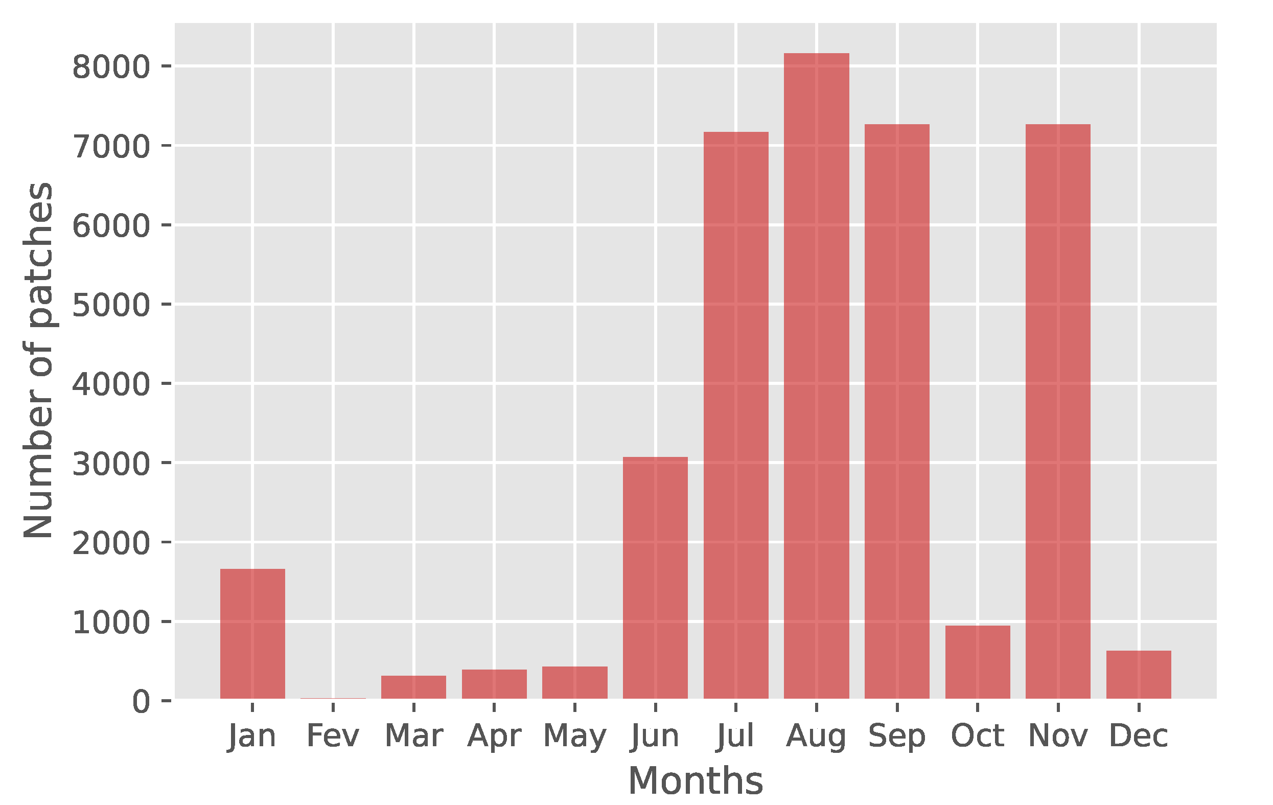
MultiSenGE [36] provides a set of functions to extract multiple Sentinel-1 and Sentinel-2 time series information for each patch. For example, it is possible to extract all patches that have at least one Sentinel-2 image associated for several months. Thus, we chose to explore the dataset to find the best compromise between temporal and spatial diversity. From Figure 2, we note that the dataset contains few images for winter and early spring.
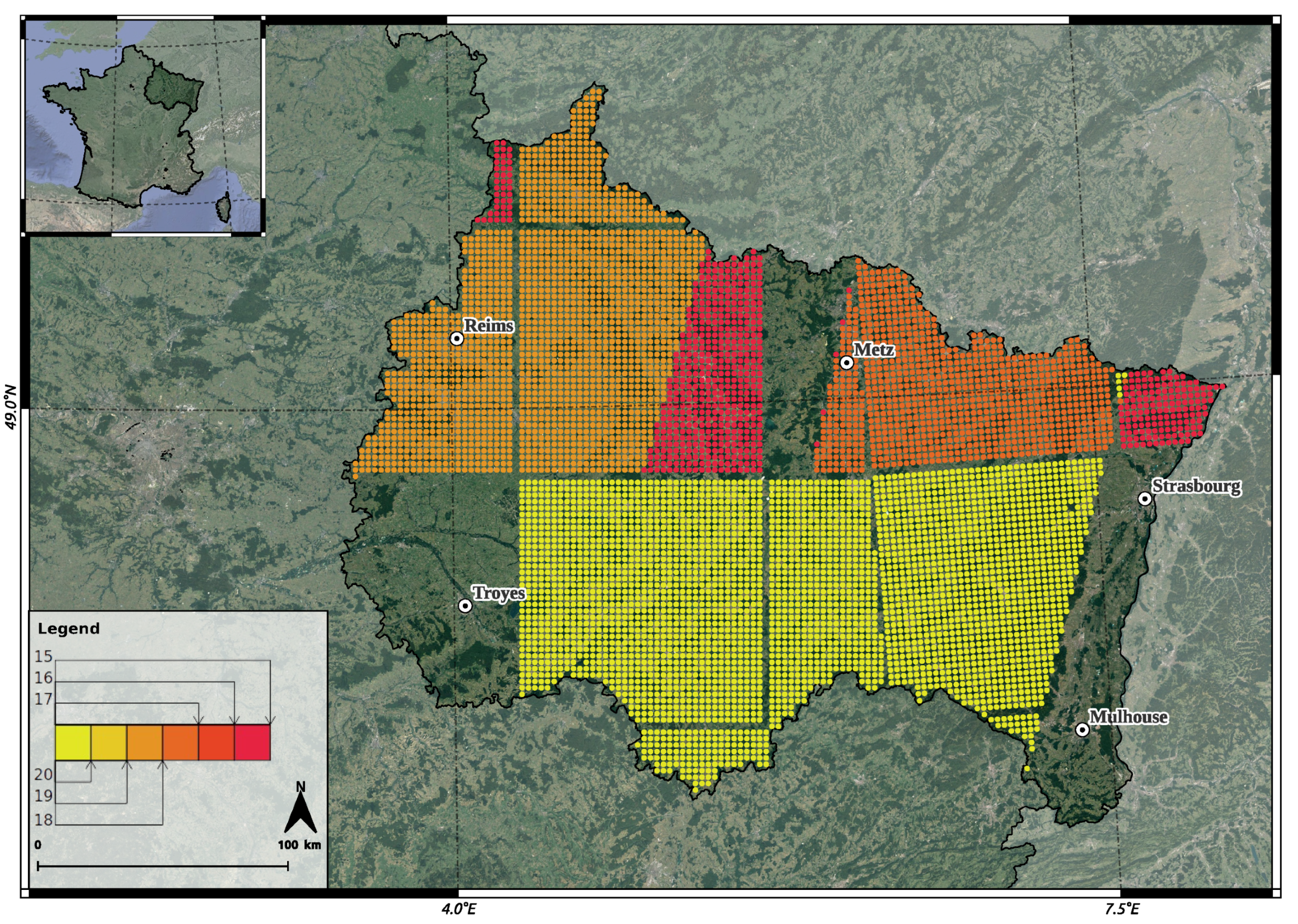
Therefore, we decided to select patches for July (07), August (08), September (09), and November (11) to have the highest number of patches (Figure 2). To obtain images with a regular time-lapse, a constraint on the number of days between two consecutive months is applied to select the patches. To help in the choice of the best configuration of number and spatial diversity on a large region, we propose a web-page (http://romainwenger.fr/visu-multisenge/index.html, accessed on 5 September 2022) allowing displaying it by mapping the center of the patch (Figure 3).
We decided to select 17 days between two consecutive months to maximize the number of patches available (Table 1) as recommended in [33]. In a previous work, some tests were made on the contribution of a larger number of Sentinel-2 dates. The first results showed that four dates without clouds are relevant to reduce uncertainties in a classification result compared to a larger number of dates which can increase them [37]. Moreover, the choice of this gap between two consecutive months is the best compromise between the number of patches and the spatial distribution of patches.
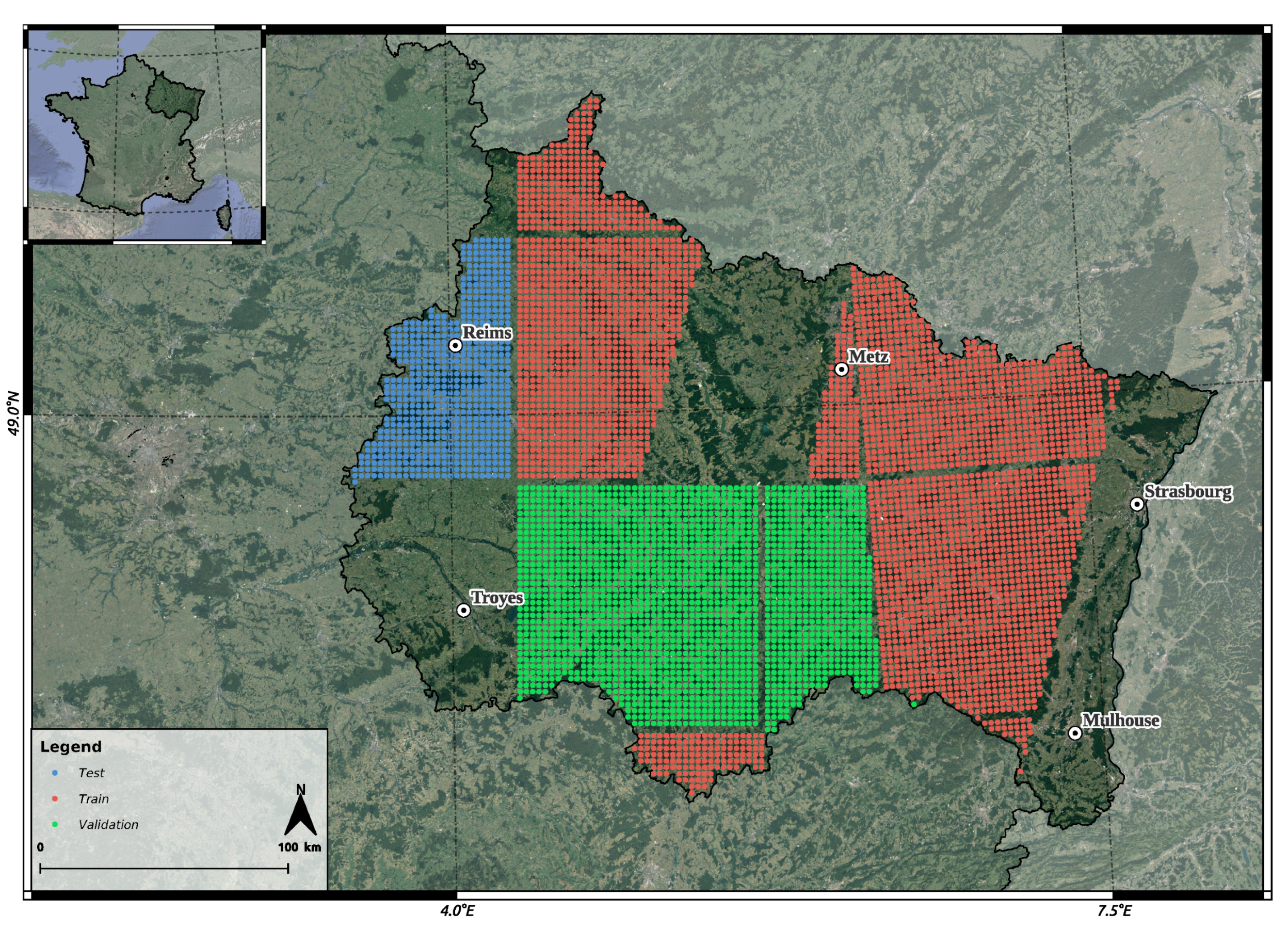
A sampling of the training, validation, and test sets is done according to a geographical stratification [38] following Sentinel-2 tiling (Figure 4). Patches from tiles T31UFP and T31UGP are chosen for the validation set, T31UEQ for the test set, and all other available tiles for the training set (T32UMV, T32ULU, T32TLT, T31UGQ, T31TFN, T31UFQ, T31UFR). In total, there are 3369 patches for training (before data augmentation), 1911 patches for validation, and 610 patches for the test set.
Particular attention is accorded to keep the proportion of classes in the training and validation datasets. The patches from the test set are centered on Reims, another large city in the west of the region, allowing us to assess the performance of your model for urban thematic classes.

2.3. Reference Data Typology

The reference land cover dataset of MultiSenGE is described in 14 semantic classes. Following the choice of the different sets by geographical stratification, some classes are not homogeneously distributed in all the sets; for instance Orchards (8), Groces and Hedges (10), Open Spaces, Mineral (12), and Wetlands (13) represent mostly under 1% for the total dataset surface (Table 2).
To reduce the unbalanced distribution of classes, we decided to merge some of them: (7) and (8) into a Vineyards and Orchards class, (10), (11) and (12) to create a class with Forests and semi-natural areas, and (13) and (14) for all the Water Surfaces (Table 2). Two different groupings are proposed on the baseline data, the first with 10 classes and the second with 6 classes to increase the number of thematic classes into several UFs (Table 3). The assumption is that with 10 land cover classes, the urban surfaces will be much better classified than with 6 land cover classes because the confusion between the natural classes will be reduced.
Even with these typologies in 6 or 10 classes, there are still some unbalanced classes (with less than 1% of the total land cover), especially for UFs classes (Dense Built-Up(1), Specialized but Vegetative Areas (4) and Large Scale Networks (5)). We have chosen not to merge these urban classes as they have already been used in several existing works [1,7,19,36]. Indeed, these UFs semantic classes are often useful for urban planning, and decision-makers and are generic enough to map western cities.

3. Models

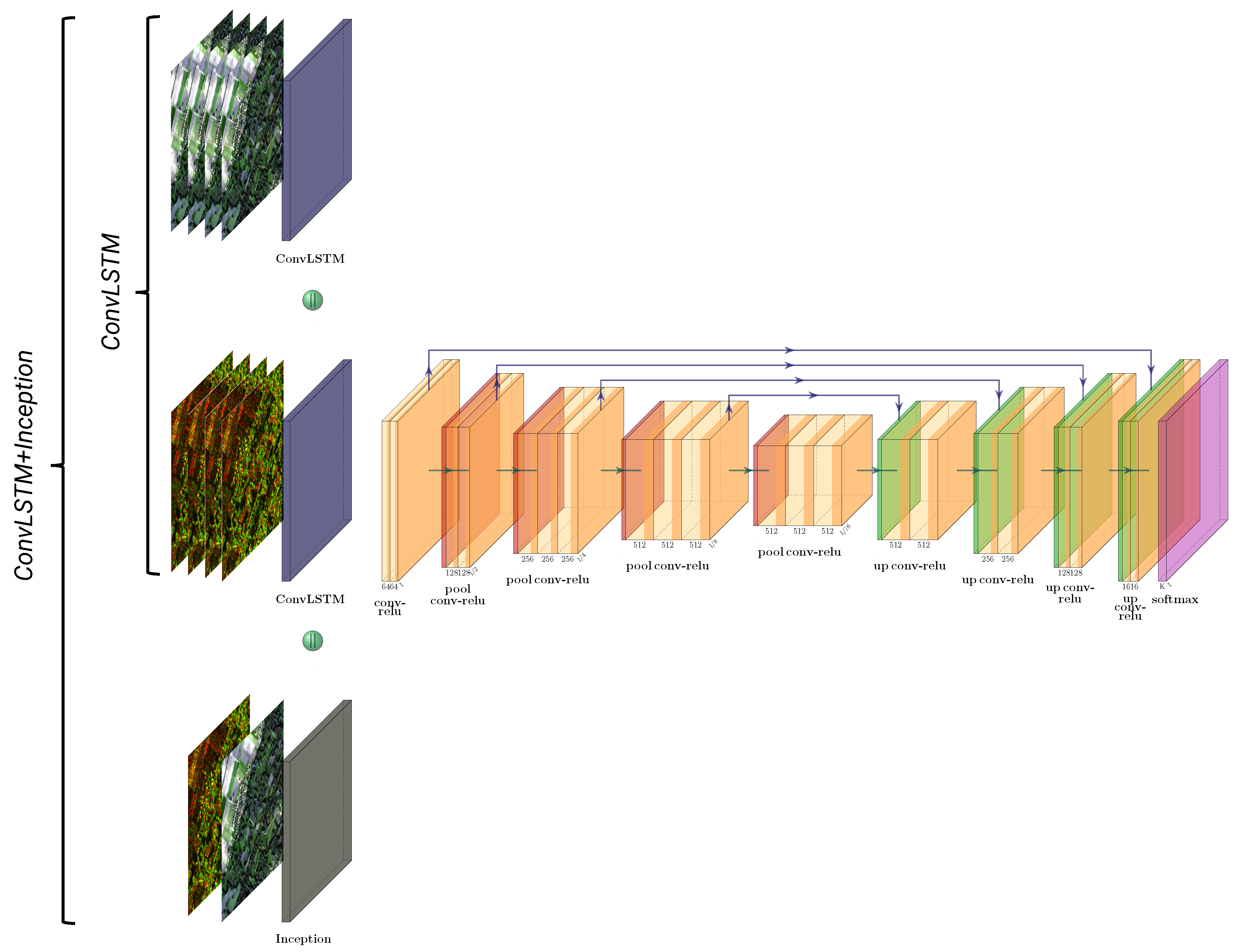
In this section, we explain the two architectures (Figure 5) used for the different experiments. The first method uses a ConvLSTM module allowing the extraction of spatio-temporal features and takes as input the Sentinel-1 and Sentinel-2 multitemporal series (Section 3.1). The second method is an extension of the first one with the addition of a naive inception module for the extraction of spatial features based on filters of three different sizes in Section 3.2. Features computed for the two models are then concatenated and added as an input to a U-Net to obtain a LULC classification. These two methods were compared by taking as input different parameters described below (Section 3.3). Furthermore, evaluation metrics used in this study are presented at the end of the section (Section 3.5).

3.1. Spatio-Temporal Feature Extractor: ConvLSTM-S1/S2

The first method, ConvLSTM (Figure 5), is implemented by taking as the primary layer a ConvLSTM to extract spatio-temporal features that will be taken as input to a U-Net network [17,39]. The ConvLSTM layer is an extension of the LSTM which only computed temporal features without taking into account the spatial information of the 2D data. It is then that the ConvLSTM layer was set up which takes in input 5D data of the following form:
X n × T × R × C × C
where X n represents the nth image, T the temporal dimension, R the number of rows, C the number of columns and C the number of channels.
We used 256 × 256 patches with a temporal depth of 4 and 10 spectral bands. Our input data will therefore be of the following form:
X n × 4 × 256 × 256 × 10
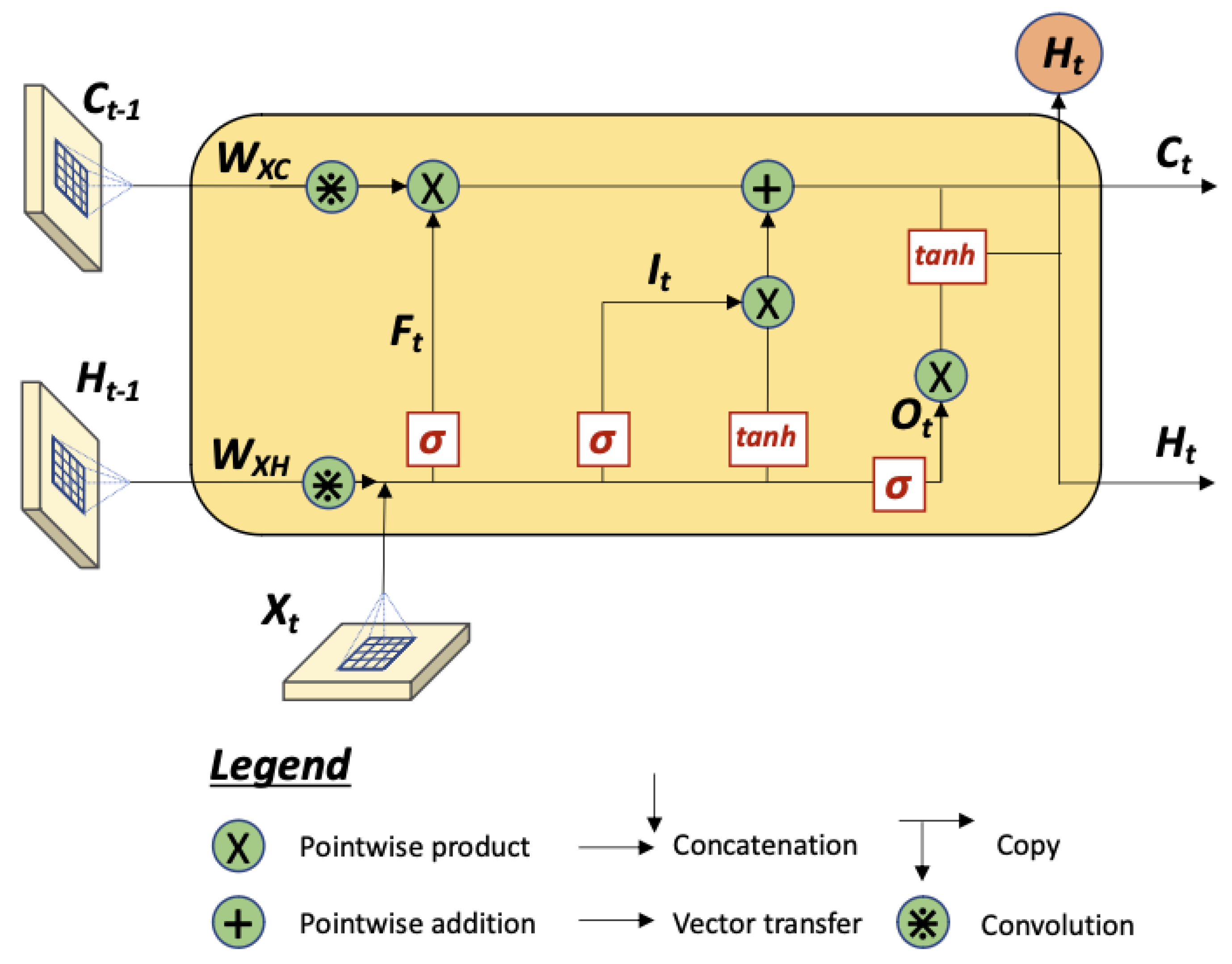
The general structure of ConvLSTM (Figure 6) consists of taking as input X 1 , , X t and returning as output spatio-temporal features which are 4D tensors. In Equation (3), which describes the ConvLSTM layer, ∗ denotes the convolutional operator and ⊙ the Hadamard product [31].
i t = σ W x i X t + W h i H t 1 + W c i C t 1 + b i f t = σ W x f X t + W h f H t 1 + W c f C t 1 + b f C t = f t C t 1 + i t tan h W x c X t + W h c H t 1 + b c o t = σ W x o X t + W h o H t 1 + W c o C t + b o H t = o t tan h C t
In our case, we used a kernel of 3 × 3 and a filter size of 32. This layer is used for the Sentinel-1 time series, the Sentinel-2 time series, and finally for the two SAR and optical series together with a concatenation of the spatio-temporal features from each of the branches before input to the U-Net [17] model.
We chose to use a U-Net which is widely used for semantic segmentation with or without changes in the basic architecture [40,41,42]. This network has the particularity to reduce the spatial information for the contracting part while increasing the features and combining the spatial and geographical information for the expensive part. The first part consists of a succession of convolutions followed by a ReLu (Rectified Linear Unit, f ( x ) = m a x ( 0 , x ) ) and a MaxPooling operation. The second part of the network is also composed of a series of convolutions, but this time it is followed by an UpSampling layer. At each pass through the network, the spatial resolution is initially reduced thanks to the downsampling layers, while the "spectral" information is increased. A second time, the "spectral" information is reduced to gain spatial information thanks to the UpSamplaing layer. VGG-16 has been chosen as a backbone because it is a good compromise between the complexity and the size of the network to limit overfitting. At the end of the network, a softmax function calculate the probability of each pixel. This network has been implemented thanks to [39].

3.2. Spatio-Spectral-Temporal Feature Extractor: ConvLSTM+Inception-S1S2

The second method, ConvLSTM+Inception (Figure 5), consists of adding, in addition to the ConvLSTM modules, a Naive Inception module (Figure 7) which allows performing three 2D convolutions with filters of 1 × 1 , 3 × 3 and 5 × 5 followed by a MaxPooling which allow limiting the overfitting and to save inputs in the model. Each 2D convolution of the model is followed by a ReLu (Rectified Linear Unit, f ( x ) = m a x ( 0 , x ) ) at the end of the 2D convolution operations, the features extracted from the module are concatenated as well as the spatio-temporal features extracted from the ConvLSTM Sentinel-1 and Sentinel-2 modules. This second method applies only to the Sentinel-1 and Sentinel-2 time series for each ConvLSTM module as well as the first date of the series, in this case, the first date of July for the optical and SAR modules, which are concatenated before being passed into the Naive Inception module to extract spatio-spectral features.
The U-Net used in the first part was also used in this one by taking as input the stack of features computed by the Inception module and the two ConvLSTM layers. This architecture was used for two experiments with, respectively, 6 and 10 classes as described in Section 2.3.

3.3. Experimentation Details

Four main experiments (Table 4) are developed to test the contribution of each sensor for spatio-temporal feature extraction and an additional one that adds the spatio-spectral feature extractor combined with the spatio-temporal extractor. These tests are run for both 6 classes and 10 classes to explore the influence of a more diverse dataset which would offer less confusion and a better classification of both UFs and natural classes.

3.4. Implementation Details

Due to the imbalance of the dataset (Table 2), we chose to implement a Weighted Categorical Cross Entropy allowing us to assign a higher weight to the less balanced classes. The weight of each class is defined as the inverse of the frequency of the class [19,27] and is commonly used in multiclass remote sensing classification [43,44]. As demonstrated by [45], Categorical Cross Entropy loss performs better than some other loss functions for semantic segmentation tasks. This method allows forcing the network to pay more attention to the less represented classes in the reference data (e.g., Built-Up (Class 1), Specialized However, Vegetative Areas (Class 4), or Large Scale Networks (5)). Furthermore, Adam is selected as an optimizer [46] as it performs better in remote sensing data than all others [47,48,49,50].
The Sentinel-1 and Sentinel-2 data are normalized to the multi-temporal information of each band using the following formula:
n = b b ¯ σ b
where n represents the normalized spectral band, b the reflectance values of each multitemporal spectral bands, b ¯ the mean of the multitemporal reflectance values, and σ b the standard deviation of the multitemporal reflectance values.
We chose to implement three different methods of data augmentation based on either 90, 180, or 270-degree rotation up/down flips and left/right flips. The training dataset is augmented to 75%. EarlyStopping, present in the Keras (https://www.tensorflow.org/api_docs/python/tf/keras accessed on 27 May 2022) library, is used with a patience of 20 epochs to avoid any overfitting. Adam optimizer is used with a LR of 10 3 and we reduce it by a factor of 0.1 after 5 epochs each time a plateau is reached thanks to the ReduceLROnPlateau method. Every Python code were run on a GPU cluster using 3 RTX6000 with 24 GB of VRAM each (72 GB in total). This allowed us to use a batch size of 16 for each run proposed in the paper.

3.5. Evaluation Metrics

Three evaluation metrics are used to assess the overall performance of the models and each class studied: F 1 S c o r e , Recall, Precision [51] and Cohen’s Kappa.
Precision score, also known as User’s Accuracy, allows extracting the number of correctly classified pixels in the classified image and is calculated as follows:
P r e c i s i o n = T P T P + F P
Recall score, also known as Producer’s Accuracy, allows extracting the percentage of well-predicted positives compared to all positives and is calculated as follows:
R e c a l l = T P T P + F N
F 1 S c o r e , also known as Dice, is the harmonic mean between the two previously explained metrics, Precision and Recall. It is calculated as follows:
F 1 S c o r e = 2 × P r e c i s i o n × R e c a l l P r e c i s i o n + R e c a l l
We also chose to compute each weighted metric for all classes to globally evaluate each model. They are calculated taking the mean of all class while considering each class’s support.
Cohen’s Kappa measure the level of agreement between two annotations.
κ = P o P e 1 P e .
where P o defined the empirical probability of agreement (also known as the observed agreement ratio) and P e the expected agreement.

4. Results

This section presents the results obtained for the two methods developed over the test dataset. The test data set is independent of the training set and the validation set and includes all available patches for the T31UEQ tile, as seen in Section 2.2. First, we present the results for six LULC classes in Section 4.1 then the results for 10 LULC classes in Section 4.2 and finally we compare UFs classification results between 6 and 10 LULC classification methods for UFs in Section 4.3.

4.1. 6 Classes Results

All the results for the six semantic classes are compiled in Table 5. For these first experiments, we study the influence of the addition of different sensors (Sentinel-1 and Sentinel-2), for one date per month for July, August, September, and November. We notice that with 6sixLULC classes, it is difficult for the tested methods to have a convergence of the scores for all the classes. We notice that the ConvLSTM-S1 method offers the best F 1 S c o r e with 0.1344 for the classification of the Specialized but Vegetative Areas (4).
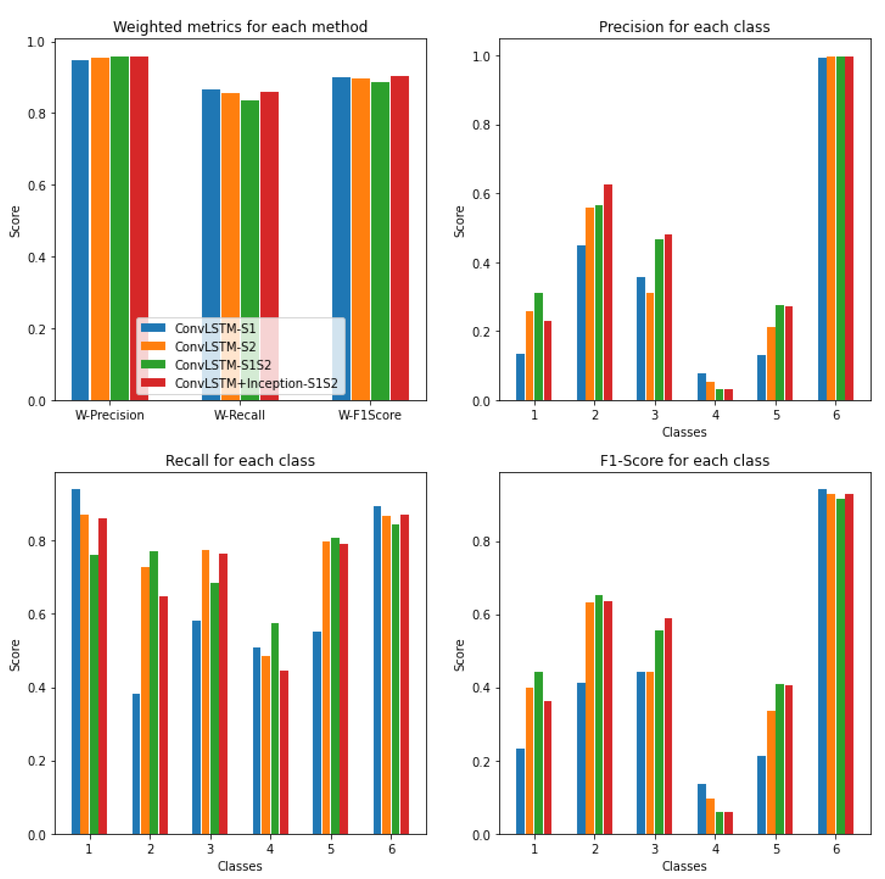
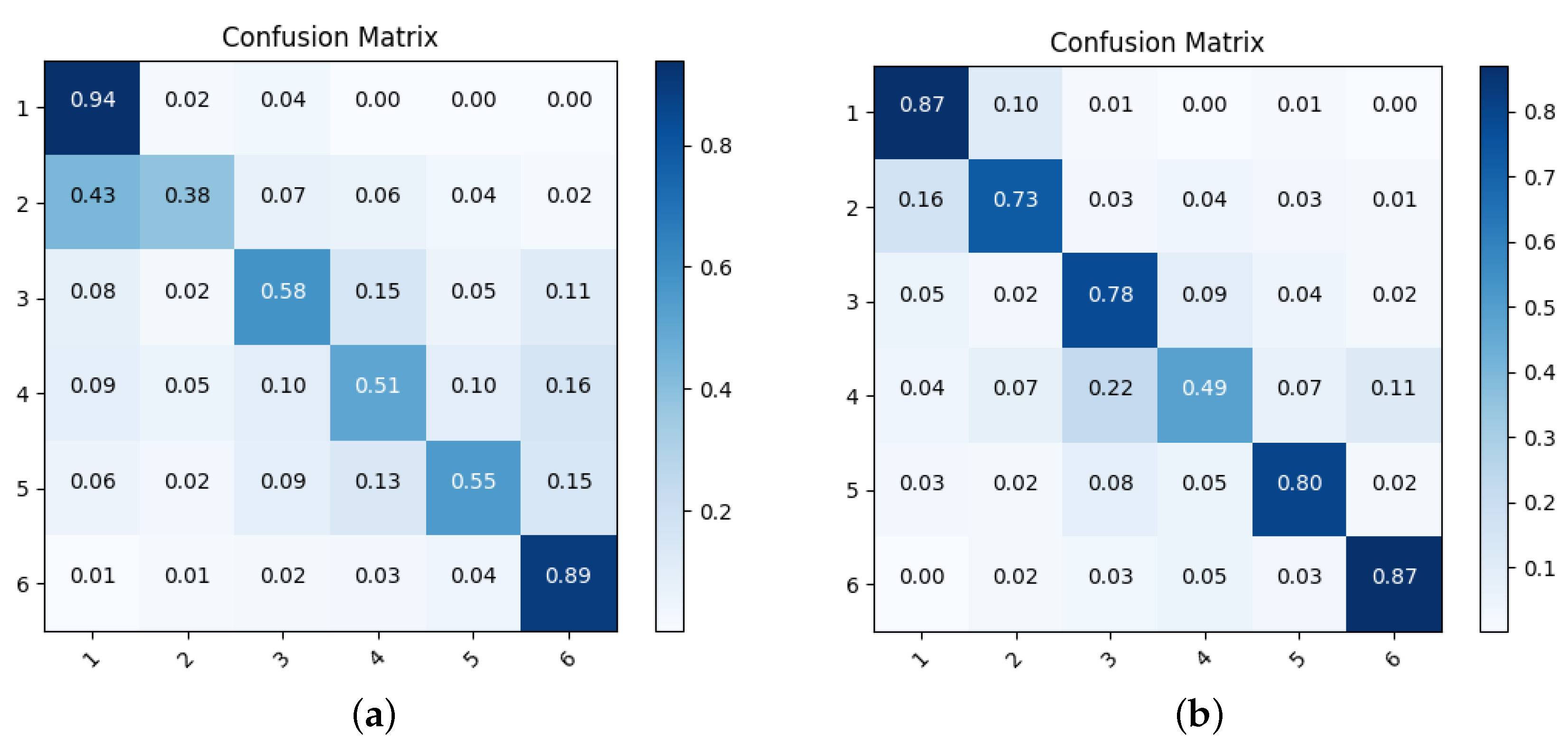
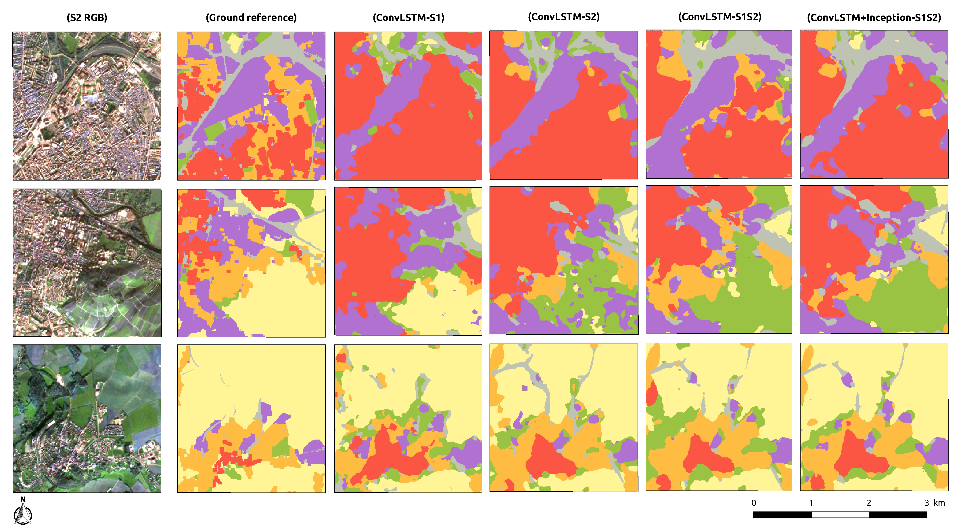
The addition of multitemporal and multimodal data for the extraction of spatio-temporal features (ConvLSTM-S1S2 method) allows obtaining a large part of the best Recall score and F 1 S c o r e , especially for Dense Built-Up (1), Sparse Built-Up (2) and Large Scale Networks (5). The addition of the Inception module for the extraction of spatio-spectral features (ConvLSTM+Inception-S1S2) does not allow a significant improvement of the classes, even if in terms of Weighted- F 1 S c o r e , it is very close to the ConvLSTM-S1S2 method with 0.8875 against 0.9018 for the latter (Table 5 and Figure A1). On the other hand, ConvLSTM+Inception-S1S2 obtains the best Weighted-Precision and Weighted- F 1 S c o r e with 0.9591 and 0.9018. The confusion matrix (Figure A2) informs us about a strong confusion between Specialized However, Vegetative Areas (4) and Non-urban areas (6), probably due to the imbalanced dataset because Non-urban areas (6) covers 92.46% of the dataset. Furthermore, it is complex to differentiate it from other natural classes as Non-urban areas (6) is the aggregation of all other natural areas. Moreover, we notice a strong confusion between Dense Built-Up (1) and Sparse Built-Up (2) which are complex classes to differentiate because their texture and spectral signature are very close at 10m. The only difference between these two UF classes is the portion of vegetation between buildings [7,19], which are close to none for Dense Built-Up (1) and are restricted to the personal garden for Sparse Built-Up (2). We can see that Recall values are systematically higher than the Precision Values whatever the method. However, the Precision value is also always higher (classes Sparse Built-Up (2) and Specialized Built-Up Areas (3)) or very similar (classes Dense Built-Up (1), Specialized However, Vegetative Areas (4) and Large Scale Networks (5)) with ConvLSTM+Inception-S1S2 than other methods. As seen in Table 6 with the Cohen’s Kappa metric, we can see that there is a very low agreement as seen with the scores between 0.3929 and 0.4223.
The visual analysis (Figure 8) is performed on three patches with different urban densities: 31UEQ_GR_7453_4112, 31UEQ_GR_6939_6682, 31UEQ_GR_3855_8481 (these patches can be viewed by downloading MultiSenGE [36]). These results confirm the statistical results where the best classifications are found for the ConvLSTM-S1S2 and ConvLSTM+Inception-S1S2 methods. We notice a better delimitation of the boundaries between UFs (class (1) to (5)) and Non-urban areas (6).

4.2. 10 Classes Results

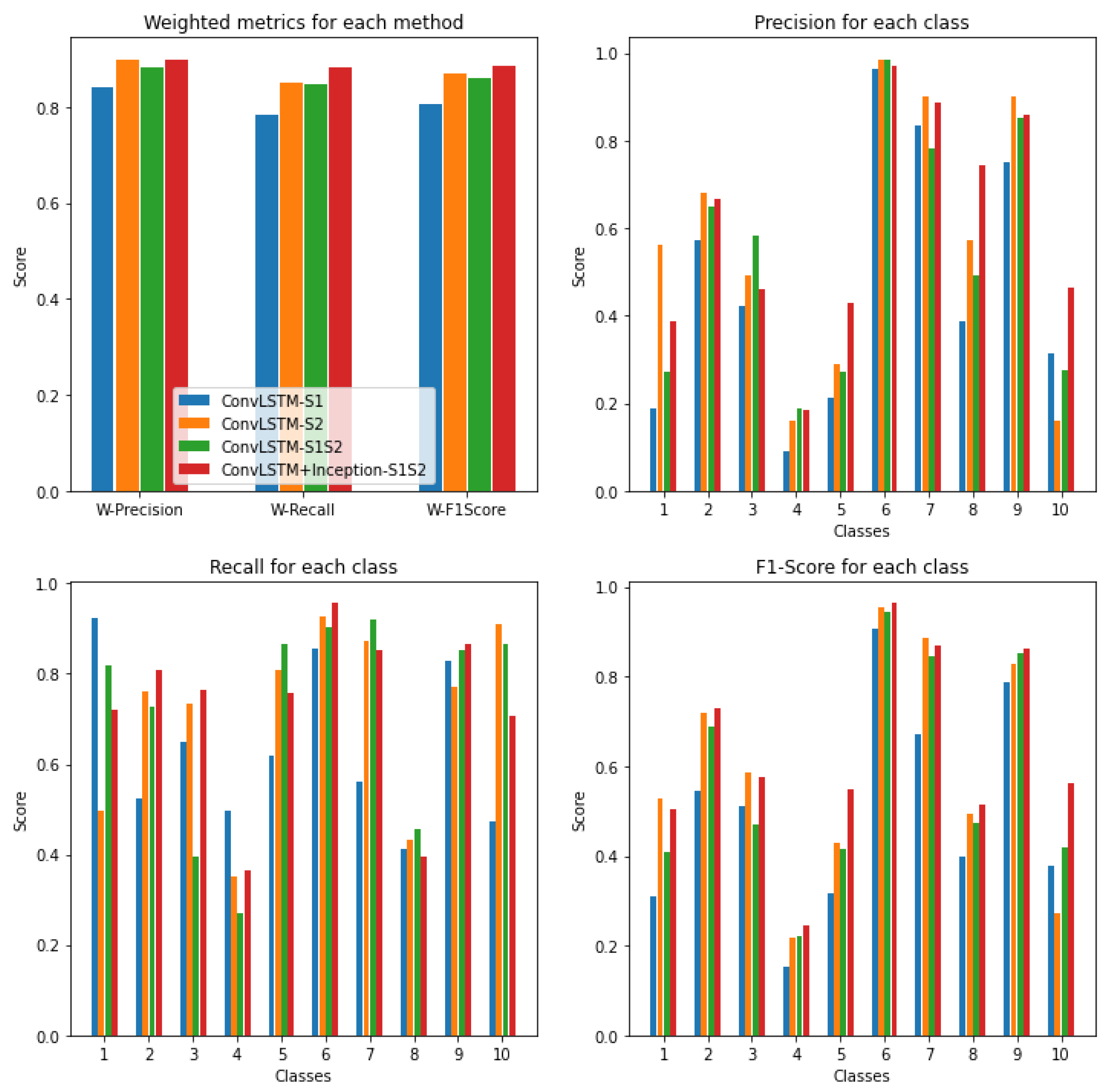
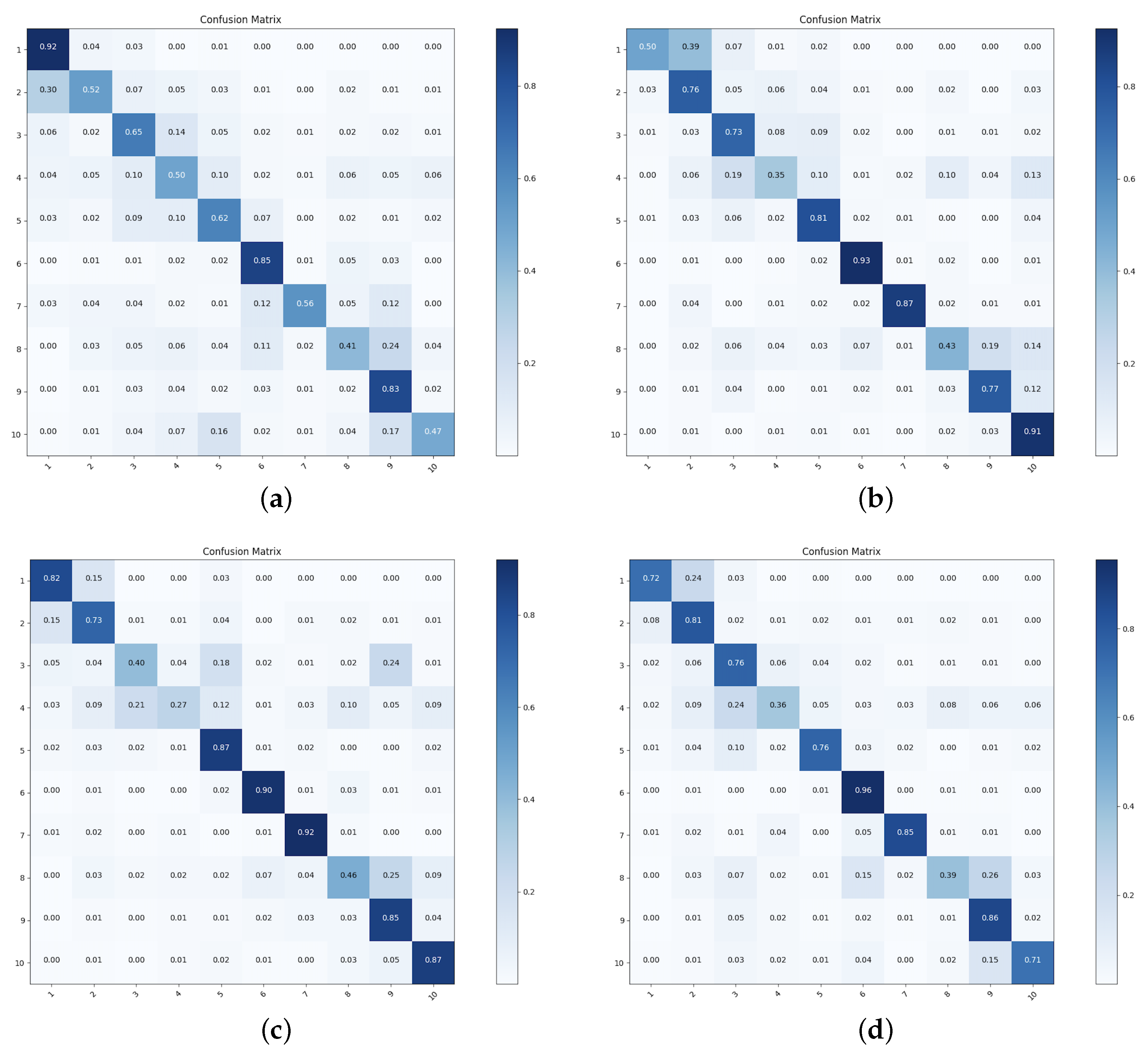
This section summarizes all quantitative and qualitative results for the 10 LULC classifications. Table 7 contains all the statistical results for the 10 classes of experiments. We notice that all the global evaluation metrics such as the accuracy, the Weighted- F 1 S c o r e and the Mean- F 1 S c o r e have the highest scores for the ConvLSTM+Inception-S1S2 method with 0.8831, 0.6373 and 0.8851, respectively. Moreover, the vast majority of the classes have a higher F 1 S c o r e for the latter. Only three classes have higher scores for another method (ConvLSTM-S2): Dense Built-Up (1), Sparse Built-Up (2) and Vineyards and Orchards (7). Moreover, this method allows better extraction of natural classes probably thanks to the spatio-spectral feature extractor (Figure A3). The analysis of the confusion matrixes (Figure A4) allows us to identify weaker confusions for the ConvLSTM+Inception-S1S2 method than for all the other methods tested. We can also notice that Recall values are always higher than Precision for almost every UF classes and method. This trend does not apply to natural classes.
As seen in Table 8, the best agreement between reference data and classification are for the ConvLSTM+Inception-S1S2 with 0.7945 for Cohen’s Kappa evaluation metric. This confirmed the best results for this method compared to others.
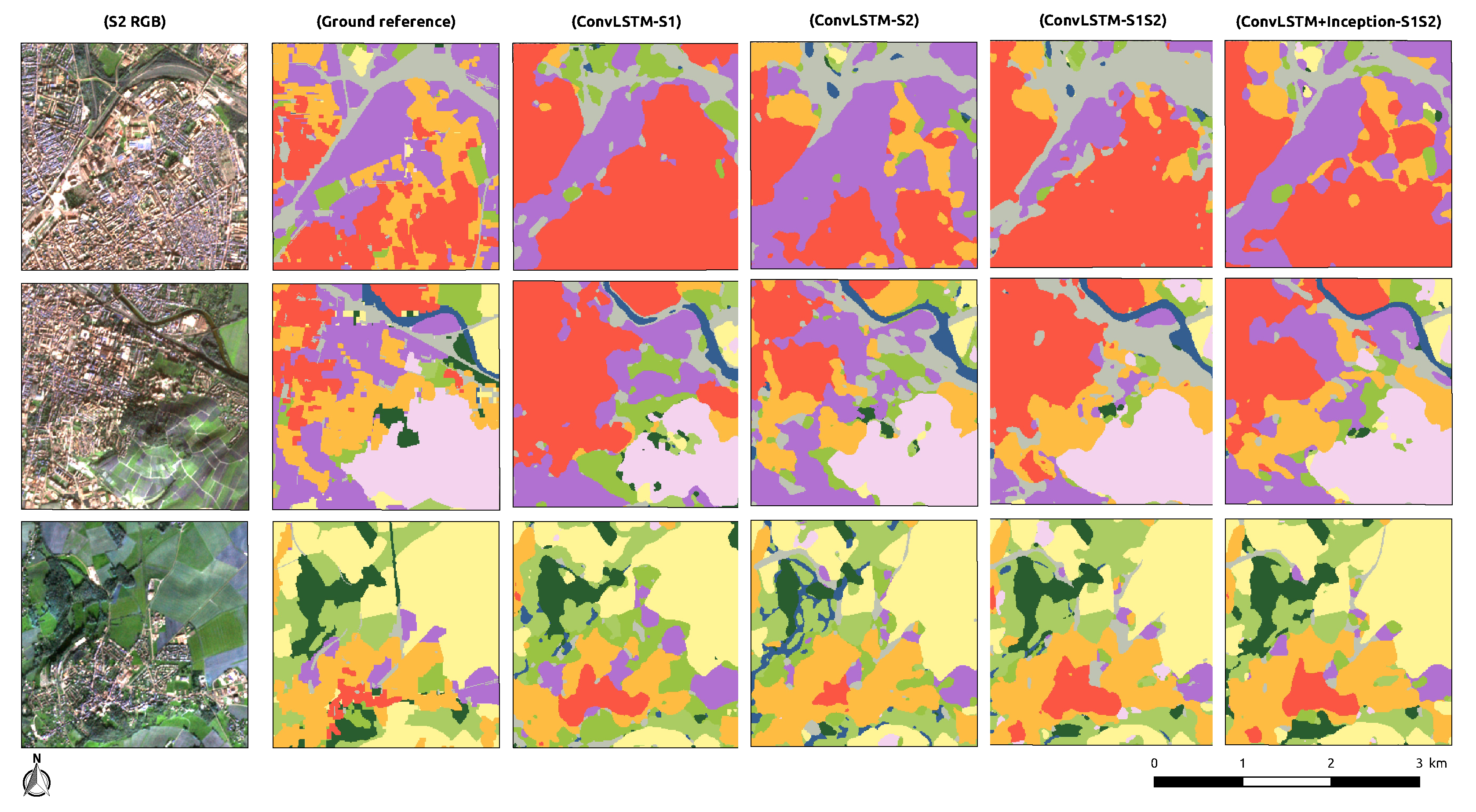
To perform the qualitative assessment for this section, we used the same patches as in Section 4.1 to compare the two approaches (31UEQ_GR_7453_4112, 31UEQ_GR_6939_6682, 31UEQ_GR_3855_8481).
The qualitative analysis allows us to observe that the Vineyard and Orchards (7) class initially strongly confused with the Specialized but vegetative Areas class (4) in the 6-class methods is correctly classified. The urban boundaries are correctly defined. We also notice that for the natural areas and more particularly the class Forest and semi-natural areas (9), the boundaries between the classes are more precise for the ConvLSTM+Inception-S1S2 method than for all the other methods. For the second best performing method (ConvLSTM-S2), a strong confusion is found between this class and the Water Surfaces (10) class. It is also interesting to note that the small roads, initially not present in the reference data, are detected for the ConvLSTM-S2 and ConvLSTM+Inception-S1S2 methods (Figure 9).

4.3. UFs Analysis

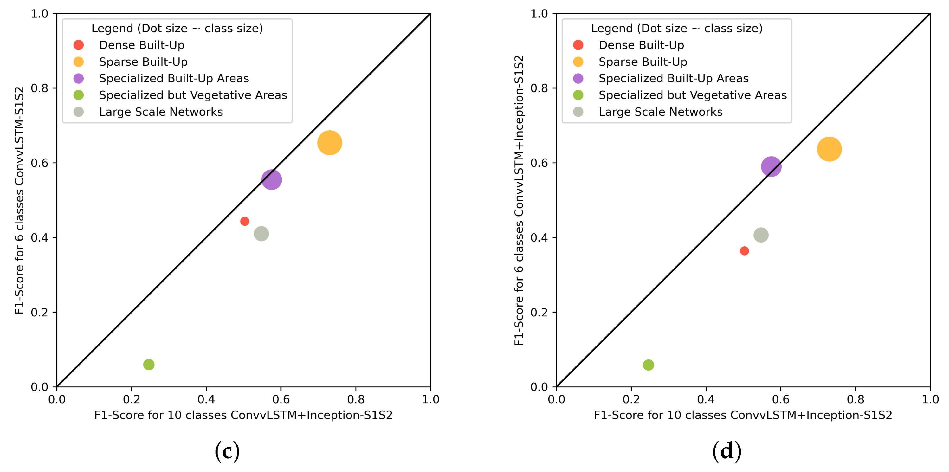
The evaluation metrics F 1 S c o r e for each class UFs are displayed on several graphs (Figure 10) for the best 10-class method and all 6-class methods. We notice that the ConvLSTM+Inception-S1S2 method for 10 class LULC classes provides better results for all five class UFs chosen for this study. Only the Specialized Built-Up Areas class (3) performs better for ConvLSTM+Inception-S1S2 at 6 classes than at 10 classes. On the other hand, all other classes are better classified for 10 classes because the confusion between them is strongly reduced. As seen in Figure 8 and Figure 9, the better performance with 10 LULC classes is particularly noticeable at the level of the urban periphery. ConvLSTM+Inception-S1S2 allows better separating the Dense Built-Up (1) and the Sparse Built-Up (2). Large Scale Networks (5) were better extracted using ConvLSTM+Inception-S1S2 and less confusion can be seen with Specialized Built-Up Areas (3) compared to other methods tested.

5. Discussion

In this paper, we developed a semantic segmentation method taking as input multitemporal and multimodal imagery from the MultiSenGE dataset. We propose a network consisting of two extractors, one for spatio-spectral features and the other for spatio-temporal features. The latter provides the best results compared to the other tested approaches. Moreover, discriminating an over-represented class improves the classification results for the studied object, in our case the UFs, reducing both intra and inter-classes confusion.

5.1. Application on UF Mapping

For UF mapping, results showed higher quantitative metrics at 10 classes using SAR and optical time series and an Inception module allowing the extraction of spatio-spectral features in addition to spatio-temporal features. This latter approach allows reducing the strong confusion between classes coming from imbalanced datasets during the 6 LULC classification. This was particularly true for Figure 8 and Figure 9 where Vineyards and Orchards (7) were strongly confused with Specialized but Vegetative Areas (4), a class that also includes scattered trees in urban parks or squares. Moreover, the results presented allowed us to see the contribution of Sentinel-1 SAR imagery thanks to the better detection of natural surfaces in the periphery of the UF. Without this acquisition mode, the confusion between the natural classes and Specialized but Vegetative Areas (4) would probably have been more important and would not have allowed a better detection of these areas.
Sentinel-2 satellite imagery provides a high spatial and high temporal coverage thanks to its temporal resolution (3 to 6 days). However, UF mapping remains challenging as these classes contains very small objects with various spectral diversity. Indeed, the distinction between UFs classes is mainly based on the amount of vegetation in each class (e.g., Dense Built-Up (1) and Sparse Built-Up (2)). On the other hand, temporal diversity provides essential information to refine the classifications as it offers the possibility to assess the evolution of the landscape and especially the vegetation through time. Results obtained in this study are superior to existing work mapping UF in several classes from Sentinel imagery [7,19].

5.2. Comparison with a State of the Art LULC Product

Compared to existing products such as OSO [1], our method is better to describe UF classes on most of the class. Indeed, using semantic segmentation instead of classical machine learning approaches (e.g., Random Forest) reduces the salt and pepper effect. Furthermore, we include a fifth class, Specialized but Vegetative Areas (4), which is almost never mapped in existing works using 10 m spatial resolution imagery (e.g., Sentinel). In fact, OSO only derives UFs in four classes, Dense Built-Up, Sparse Built-Up, Specialized Built-Up, and Large Scale Networks. For natural areas, OSO has 13 semantic classes, which is slightly higher than our approach. However, we are only experimenting with a specific region in France and a regional LULC semantic segmentation dataset, which reduce the possibilities to extend the number of classes. Due to the complex spectral diversity of the Specialized but Vegetative Areas (4) class because of the large number of objects (Trees, Grasslands, Minerals …, also included in other LULC classes), F 1 S c o r e cannot exceed 0.25. However, almost every vegetative areas inside urban areas remains to Specialized but Vegetative Areas (4) using our method. Confusions are mostly seen outside urban areas.

5.3. Network Performance

Semantic segmentation networks, and more specifically the encoder-decoder like structures, allow us to obtain a map with the spatial extent of each class (assigning to each pixel a label and taking into account the spatial context of the image). Thus, we can note a lack of precision in the border of the classes, in particular those of the UF. Moreover, the complexity and density of UF make the distinction between classes difficult, especially at 10 m spatial resolution. The geographical area, being anisotropic in nature, differences in the distribution and frequency of the classes over the territory also make the classification more complex and challenging. This could be assessed by doing pixel-wise classification and balancing each class in the dataset. Through this technique, salt and pepper noise, which was almost erased with semantic segmentation, could happen again. Weighting the loss is one of the methods that has been successful in the community to assess this challenge [19,27,43,44]. In the case of our study, it seems to be working because the least represented classes (less than 2% of all classes) reach F1-Scores above 0.5. However, this strategy seems to have difficulties for the least separable and most confused classes, such as Dense Built-Up (1) (often confused with Sparse Built-Up (2)), Specialized but Vegetative Areas (4) or Grasslands (8).
Through these experimentations, ConvLSTM+Inception-S1S2 for 10 LULC classes appears to be the best method to map UF using multitemporal and multimodal imagery. Detailing an over-represented class allowed the network to improve the results by reducing intra-class confusion. Moreover, the contribution of an Inception module and of spatio-spectral features could be one of the reasons for the improvement of the classification results. The spatial context of an image, in semantic segmentation problems, is an important aspect in classification results. The addition of this module, allowing the calculation of features according to several filter sizes, may have contributed to the results obtained. On the other hand, according to the classification results, the spatio-spectral feature extractor provides important information on the smallest objects of the territory thanks to multiple kernel filter sizes.

6. Conclusions

In this study, we demonstrated the contributions of multitemporal and multimodal imagery and the use of deep learning models allowing the extraction of spatio-spectral and spatio-temporal features for a better extraction and semantic segmentation of UF. Furthermore, the results, which demonstrate better F 1 S c o r e for the 10 classes ConvLSTM+Inception-S1S2 method, showed that it is better to segment and diversify an over-represented class composed of spectrally and texturally distinct objects. This method has also greater metrics scores thanks to the addition of a spatio-spectral feature extractor. The current scores for UF are encouraging and show that combining and extracting different types of features and balancing the initial dataset provides better results by reducing confusion between the classes studied (Figure 9, Figure 10 and Figure A3). The developed methods could be used in large-scale LULC classification to study their genericity under different scenarios at different spatial scales (e.g., over France and/or Europe). For example, for cities slightly different than western cities, transfer learning could be applied and compared to a network trained from scratch. To increase the accuracy of the classifications, one of the perspectives could be to add an image with a very high spatial resolution (e.g., Pléiades or Spot6/7) and to merge the features from the multi-temporal optical and SAR images and very high spatial resolution. Furthermore, we would like to explore spatial and temporal inference to cover large territories and produce a land cover map that may be included in climatic models to characterize Local Climate Zone (LCZ).

Author Contributions

Conceptualization, R.W., A.P., J.W. and G.F.; methodology, R.W., A.P., J.W. and G.F.; software, R.W.; validation, A.P., J.W. and G.F.; formal analysis, R.W., A.P., J.W. and G.F.; resources, A.P.; data curation, R.W.; writing—original draft preparation, R.W.; writing—review and editing, R.W., A.P., J.W., G.F. and L.I.; funding acquisition, A.P. All authors have read and agreed to the published version of the manuscript.

Funding

This research is part of the PhD Thesis supported by the French funded project ANR TIMES ‘High-performance processing techniques for mapping and monitoring environmental changes from massive, heterogeneous and high frequency data times series’ [ANR-17-CE23-0015] and by the French TOSCA project AIMCEE [CNES, 2019–2022].

Data Availability Statement

MultiSenGE dataset has been downloaded through Zenodo [52]. The code used to extract MultiSenGE temporal patches can be found on GitHub [https://github.com/r-wenger/MultiSenGE-Tools, accessed on 8 June 2022]. Models source code can be accessible on demand.

Acknowledgments

We would like to thank the computer center Mesocentre Unistra for providing the calculation resources. We also would like to thanks [53] for their awesome LaTex neural network design library.

Conflicts of Interest

The authors declare no conflict of interest.

Abbreviations

The following abbreviations are used in this manuscript:
CNNConvolutional Neural Network
GRDGround Range Detection
IGNInstitut Géofgraphique National
LRLearning Rate
LULCLand Use Land Cover
SLCSingle Look Complex
UFUrban Fabrics

Appendix A

Figure A1. Bar plot results of all methods for the test zone located in the west of the Grand-Est region for 6 semantic classes.
Remotesensing 15 00151 g0a1
Figure A2. Confusion matrix computed over the test dataset for every method for 6 semantic LULC classes. (a) Confusion matrix for ConvLSTM-S1. (b) Confusion matrix for ConvLSTM-S2. (c) Confusion matrix for ConvLSTM-S1S2. (d) Confusion matrix for ConvLSTM+Inception-S1S2.
Remotesensing 15 00151 g0a2aRemotesensing 15 00151 g0a2b
Figure A3. Bar plot results of all methods for the test zone located in the west of the Grand-Est region for 10 semantic classes.
Remotesensing 15 00151 g0a3
Figure A4. Confusion matrix computed over the test dataset for every method for 10 semantic LULC classes. (a) Confusion matrix for ConvLSTM-S1. (b) Confusion matrix for ConvLSTM-S2. (c) Confusion matrix for ConvLSTM-S1S2. (d) Confusion matrix for ConvLSTM+Inception-S1S2.
Remotesensing 15 00151 g0a4

References

  1. Inglada, J.; Vincent, A.; Arias, M.; Tardy, B.; Morin, D.; Rodes, I. Operational High Resolution Land Cover Map Production at the Country Scale Using Satellite Image Time Series. Remote Sens. 2017, 9, 95. [Google Scholar] [CrossRef] [Green Version]
  2. Zanaga, D.; Van De Kerchove, R.; De Keersmaecker, W.; Souverijns, N.; Brockmann, C.; Quast, R.; Wevers, J.; Grosu, A.; Paccini, A.; Vergnaud, S.; et al. ESA WorldCover 10 m 2020 v100. 2021. Available online: https://zenodo.org/record/5571936 (accessed on 10 June 2022).
  3. Brown, C.F.; Brumby, S.P.; Guzder-Williams, B.; Birch, T.; Hyde, S.B.; Mazzariello, J.; Czerwinski, W.; Pasquarella, V.J.; Haertel, R.; Ilyushchenko, S.; et al. Dynamic World, Near real-time global 10 m land use land cover mapping. Sci. Data 2022, 9, 1–17. [Google Scholar] [CrossRef]
  4. Karra, K.; Kontgis, C.; Statman-Weil, Z.; Mazzariello, J.C.; Mathis, M.; Brumby, S.P. Global land use/land cover with Sentinel 2 and deep learning. In Proceedings of the 2021 IEEE International Geoscience and Remote Sensing Symposium IGARSS, Brussels, Belgium, 11–16 July 2021; IEEE: New York, NY, USA, 2021; pp. 4704–4707. [Google Scholar]
  5. Guo, X.; Zhang, C.; Luo, W.; Yang, J.; Yang, M. Urban Impervious Surface Extraction Based on Multi-Features and Random Forest. IEEE Access 2020, 8, 226609–226623. [Google Scholar] [CrossRef]
  6. Yang, X.; Li, Y.; Luo, Z.; Chan, P.W. The urban cool island phenomenon in a high-rise high-density city and its mechanisms. Int. J. Climatol. 2017, 37, 890–904. [Google Scholar] [CrossRef] [Green Version]
  7. El Mendili, L.; Puissant, A.; Chougrad, M.; Sebari, I. Towards a Multi-Temporal Deep Learning Approach for Mapping Urban Fabric Using Sentinel 2 Images. Remote Sens. 2020, 12, 423. [Google Scholar] [CrossRef] [Green Version]
  8. Li, J.; Narayanan, R. A shape-based approach to change detection of lakes using time series remote sensing images. IEEE Trans. Geosci. Remote Sens. 2003, 41, 2466–2477. [Google Scholar] [CrossRef]
  9. Karasiak, N.; Sheeren, D.; Fauvel, M.; Willm, J.; Dejoux, J.F.; Monteil, C. Mapping tree species of forests in southwest France using Sentinel-2 image time series. In Proceedings of the 2017 9th International Workshop on the Analysis of Multitemporal Remote Sensing Images (MultiTemp), Brugge, Belgium, 27–29 June 2017; pp. 1–4. [Google Scholar] [CrossRef]
  10. Li, Q.; Wang, C.; Zhang, B.; Lu, L. Object-Based Crop Classification with Landsat-MODIS Enhanced Time-Series Data. Remote Sens. 2015, 7, 16091–16107. [Google Scholar] [CrossRef] [Green Version]
  11. Praticò, S.; Solano, F.; Di Fazio, S.; Modica, G. Machine Learning Classification of Mediterranean Forest Habitats in Google Earth Engine Based on Seasonal Sentinel-2 Time-Series and Input Image Composition Optimisation. Remote Sens. 2021, 13, 586. [Google Scholar] [CrossRef]
  12. Zhou, T.; Zhao, M.; Sun, C.; Pan, J. Exploring the Impact of Seasonality on Urban Land-Cover Mapping Using Multi-Season Sentinel-1A and GF-1 WFV Images in a Subtropical Monsoon-Climate Region. ISPRS Int. J. Geo-Inf. 2018, 7, 3. [Google Scholar] [CrossRef]
  13. Ma, L.; Liu, Y.; Zhang, X.; Ye, Y.; Yin, G.; Johnson, B.A. Deep learning in remote sensing applications: A meta-analysis and review. ISPRS J. Photogramm. Remote Sens. 2019, 152, 166–177. [Google Scholar] [CrossRef]
  14. Pelletier, C.; Webb, G.I.; Petitjean, F. Temporal convolutional neural network for the classification of satellite image time series. Remote Sens. 2019, 11, 523. [Google Scholar] [CrossRef] [Green Version]
  15. Zhang, P.; Ke, Y.; Zhang, Z.; Wang, M.; Li, P.; Zhang, S. Urban Land Use and Land Cover Classification Using Novel Deep Learning Models Based on High Spatial Resolution Satellite Imagery. Sensors 2018, 18, 3717. [Google Scholar] [CrossRef] [Green Version]
  16. Hafner, S.; Ban, Y.; Nascetti, A. Unsupervised domain adaptation for global urban extraction using sentinel-1 SAR and sentinel-2 MSI data. Remote Sens. Environ. 2022, 280, 113192. [Google Scholar] [CrossRef]
  17. Ronneberger, O.; Fischer, P.; Brox, T. U-Net: Convolutional Networks for Biomedical Image Segmentation. In Proceedings of the 2015 International Conference on Medical Image Computing and Computer-Assisted Intervention, Munich, Germany, 5–9 October 2015. [Google Scholar]
  18. Badrinarayanan, V.; Kendall, A.; Cipolla, R. SegNet: A Deep Convolutional Encoder-Decoder Architecture for Image Segmentation. IEEE Trans. Pattern Anal. Mach. Intell. 2017, 39, 2481–2495. [Google Scholar] [CrossRef]
  19. Wenger, R.; Puissant, A.; Weber, J.; Idoumghar, L.; Forestier, G. U-Net feature fusion for multi-class semantic segmentation of urban fabrics from Sentinel-2 imagery: An application on Grand Est Region, France. Int. J. Remote Sens. 2022, 43, 1983–2011. [Google Scholar] [CrossRef]
  20. Rußwurm, M.; Pelletier, C.; Zollner, M.; Lefèvre, S.; Körner, M. Breizhcrops: A time series dataset for crop type mapping. arXiv 2019, arXiv:1905.11893. [Google Scholar] [CrossRef]
  21. Ienco, D.; Interdonato, R.; Gaetano, R.; Ho Tong Minh, D. Combining Sentinel-1 and Sentinel-2 Satellite Image Time Series for land cover mapping via a multi-source deep learning architecture. ISPRS J. Photogramm. Remote Sens. 2019, 158, 11–22. [Google Scholar] [CrossRef]
  22. Ghassemian, H. A review of remote sensing image fusion methods. Inf. Fusion 2016, 32, 75–89. [Google Scholar] [CrossRef]
  23. Hedayati, P.; Bargiel, D. Fusion of Sentinel-1 and Sentinel-2 Images for Classification of Agricultural Areas Using a Novel Classification Approach. In Proceedings of the IGARSS 2018—2018 IEEE International Geoscience and Remote Sensing Symposium, Valencia, Spain, 22–27 July 2018; pp. 6643–6646. [Google Scholar] [CrossRef]
  24. Inglada, J.; Arias, M.; Tardy, B.; Morin, D.; Valero, S.; Hagolle, O.; Dedieu, G.; Sepulcre, G.; Bontemps, S.; Defourny, P. Benchmarking of algorithms for crop type land-cover maps using Sentinel-2 image time series. In Proceedings of the 2015 IEEE International Geoscience and Remote Sensing Symposium (IGARSS), Milan, Italy, 26–31 July 2015; pp. 3993–3996. [Google Scholar] [CrossRef]
  25. Smets, P. What is Dempster-Shafer’s model. In Advances in the Dempster-Shafer Theory of Evidence; John Wiley & Sons, Inc.: New York, NY, USA, 1994; Volume 34. [Google Scholar]
  26. Clerici, N.; Calderón, C.A.V.; Posada, J.M. Fusion of Sentinel-1A and Sentinel-2A data for land cover mapping: A case study in the lower Magdalena region, Colombia. J. Maps 2017, 13, 718–726. [Google Scholar] [CrossRef] [Green Version]
  27. Audebert, N.; Le Saux, B.; Lefèvre, S. Beyond RGB: Very high resolution urban remote sensing with multimodal deep networks. ISPRS J. Photogramm. Remote Sens. 2018, 140, 20–32. [Google Scholar] [CrossRef] [Green Version]
  28. Liu, J.; Gong, M.; Qin, K.; Zhang, P. A Deep Convolutional Coupling Network for Change Detection Based on Heterogeneous Optical and Radar Images. IEEE Trans. Neural Netw. Learn. Syst. 2018, 29, 545–559. [Google Scholar] [CrossRef] [PubMed]
  29. Kussul, N.; Lavreniuk, M.; Skakun, S.; Shelestov, A. Deep Learning Classification of Land Cover and Crop Types Using Remote Sensing Data. IEEE Geosci. Remote Sens. Lett. 2017, 14, 778–782. [Google Scholar] [CrossRef]
  30. Pfeuffer, A.; Schulz, K.; Dietmayer, K. Semantic segmentation of video sequences with convolutional lstms. In Proceedings of the 2019 IEEE Intelligent Vehicles Symposium (IV), Paris, France, 9–12 June 2019; IEEE: New York, NY, USA, 2019; pp. 1441–1447. [Google Scholar]
  31. Shi, X.; Chen, Z.; Wang, H.; Yeung, D.Y.; Wong, W.K.; Woo, W.C. Convolutional LSTM Network: A Machine Learning Approach for Precipitation Nowcasting, 2015. arXiv 2015, arXiv:1506.04214. [Google Scholar]
  32. Wang, D.; Yang, Y.; Ning, S. DeepSTCL: A deep spatio-temporal ConvLSTM for travel demand prediction. In Proceedings of the 2018 International Joint Conference on Neural Networks (IJCNN), Rio de Janeiro, Brazil, 8–13 July 2018; IEEE: New York, NY, USA, 2018; pp. 1–8. [Google Scholar]
  33. Jamaluddin, I.; Thaipisutikul, T.; Chen, Y.N.; Chuang, C.H.; Hu, C.L. MDPrePost-Net: A Spatial-Spectral-Temporal Fully Convolutional Network for Mapping of Mangrove Degradation Affected by Hurricane Irma 2017 Using Sentinel-2 Data. Remote Sens. 2021, 13, 5042. [Google Scholar] [CrossRef]
  34. Masolele, R.N.; De Sy, V.; Herold, M.; Marcos, D.; Verbesselt, J.; Gieseke, F.; Mullissa, A.G.; Martius, C. Spatial and temporal deep learning methods for deriving land-use following deforestation: A pan-tropical case study using Landsat time series. Remote Sens. Environ. 2021, 264, 112600. [Google Scholar] [CrossRef]
  35. Chang, Y.L.; Tan, T.H.; Chen, T.H.; Chuah, J.H.; Chang, L.; Wu, M.C.; Tatini, N.B.; Ma, S.C.; Alkhaleefah, M. Spatial-Temporal Neural Network for Rice Field Classification from SAR Images. Remote Sens. 2022, 14, 1929. [Google Scholar] [CrossRef]
  36. Wenger, R.; Puissant, A.; Weber, J.; Idoumghar, L.; Forestier, G. Multisenge: A Multimodal and Multitemporal Benchmark Dataset for Land Use/Land Cover Remote Sensing Applications. ISPRS Ann. Photogramm. Remote Sens. Spat. Inf. Sci. 2022, V-3-2022, 635–640. [Google Scholar] [CrossRef]
  37. Wenger, R.; Puissant, A.; Michéa, D. Towards an annual Urban Settlement map in France at 10m spatial resolution using a method for massive streams of Sentinel-2. LIVE CNRS UMR7362, Strasbourg, France, to be submitted.
  38. Maxwell, A.E.; Warner, T.A.; Guillén, L.A. Accuracy Assessment in Convolutional Neural Network-Based Deep Learning Remote Sensing Studies—Part 2: Recommendations and Best Practices. Remote Sens. 2021, 13, 2591. [Google Scholar] [CrossRef]
  39. Yakubovskiy, P. Segmentation Models. 2019. Available online: https://github.com/qubvel/segmentation_models (accessed on 8 November 2022).
  40. Zhang, P.; Ban, Y.; Nascetti, A. Learning U-Net without forgetting for near real-time wildfire monitoring by the fusion of SAR and optical time series. Remote Sens. Environ. 2021, 261, 112467. [Google Scholar] [CrossRef]
  41. Wei, P.; Chai, D.; Lin, T.; Tang, C.; Du, M.; Huang, J. Large-scale rice mapping under different years based on time-series Sentinel-1 images using deep semantic segmentation model. ISPRS J. Photogramm. Remote Sens. 2021, 174, 198–214. [Google Scholar] [CrossRef]
  42. Neves, A.K.; Körting, T.S.; Fonseca, L.M.G.; Girolamo Neto, C.D.; Wittich, D.; Costa, G.A.O.P.; Heipke, C. Semantic Segmentation of Brazilian Savanna Vegetation Using High Spatial Resolution Satellite Data and U-Net. ISPRS Ann. Photogramm. Remote Sens. Spat. Inf. Sci. 2020, V-3-2020, 505–511. [Google Scholar] [CrossRef]
  43. Ienco, D.; Gaetano, R.; Dupaquier, C.; Maurel, P. Land Cover Classification via Multitemporal Spatial Data by Deep Recurrent Neural Networks. IEEE Geosci. Remote Sens. Lett. 2017, 14, 1685–1689. [Google Scholar] [CrossRef] [Green Version]
  44. Zhu, X.X.; Tuia, D.; Mou, L.; Xia, G.S.; Zhang, L.; Xu, F.; Fraundorfer, F. Deep Learning in Remote Sensing: A Comprehensive Review and List of Resources. IEEE Geosci. Remote Sens. Mag. 2017, 5, 8–36. [Google Scholar] [CrossRef] [Green Version]
  45. Bai, H.; Cheng, J.; Su, Y.; Liu, S.; Liu, X. Calibrated Focal Loss for Semantic Labeling of High-Resolution Remote Sensing Images. IEEE J. Sel. Top. Appl. Earth Obs. Remote Sens. 2022, 15, 6531–6547. [Google Scholar] [CrossRef]
  46. Kingma, D.P.; Ba, J. Adam: A Method for Stochastic Optimization. arXiv 2014, arXiv:1412.6980. [Google Scholar]
  47. Bera, S.; Shrivastava, V.K. Analysis of various optimizers on deep convolutional neural network model in the application of hyperspectral remote sensing image classification. Int. J. Remote Sens. 2020, 41, 2664–2683. [Google Scholar] [CrossRef]
  48. Pires de Lima, R.; Marfurt, K. Convolutional neural network for remote-sensing scene classification: Transfer learning analysis. Remote Sens. 2019, 12, 86. [Google Scholar] [CrossRef] [Green Version]
  49. Abdollahi, A.; Pradhan, B.; Sharma, G.; Maulud, K.N.A.; Alamri, A. Improving road semantic segmentation using generative adversarial network. IEEE Access 2021, 9, 64381–64392. [Google Scholar] [CrossRef]
  50. Li, H.; Li, Y.; Zhang, G.; Liu, R.; Huang, H.; Zhu, Q.; Tao, C. Global and local contrastive self-supervised learning for semantic segmentation of HR remote sensing images. IEEE Trans. Geosci. Remote Sens. 2022, 60, 1–14. [Google Scholar] [CrossRef]
  51. Maxwell, A.E.; Warner, T.A.; Guillén, L.A. Accuracy Assessment in Convolutional Neural Network-Based Deep Learning Remote Sensing Studies—Part 1: Literature Review. Remote Sens. 2021, 13, 2450. [Google Scholar] [CrossRef]
  52. Wenger, R.; Puissant, A.; Weber, J.; Idoumghar, L.; Forestier, G. A New Remote Sensing Benchmark Dataset for Machine Learning Applications: MultiSenGE, 2022. ANR-17-CE23-0015. Available online: https://zenodo.org/record/6375466#.Y6q45UwRWUk (accessed on 8 June 2022).
  53. Iqbal, H. HarisIqbal88/PlotNeuralNet v1.0.0. 2018. Available online: https://zenodo.org/record/2526396#.Y6q5CEwRWUk (accessed on 8 June 2022).
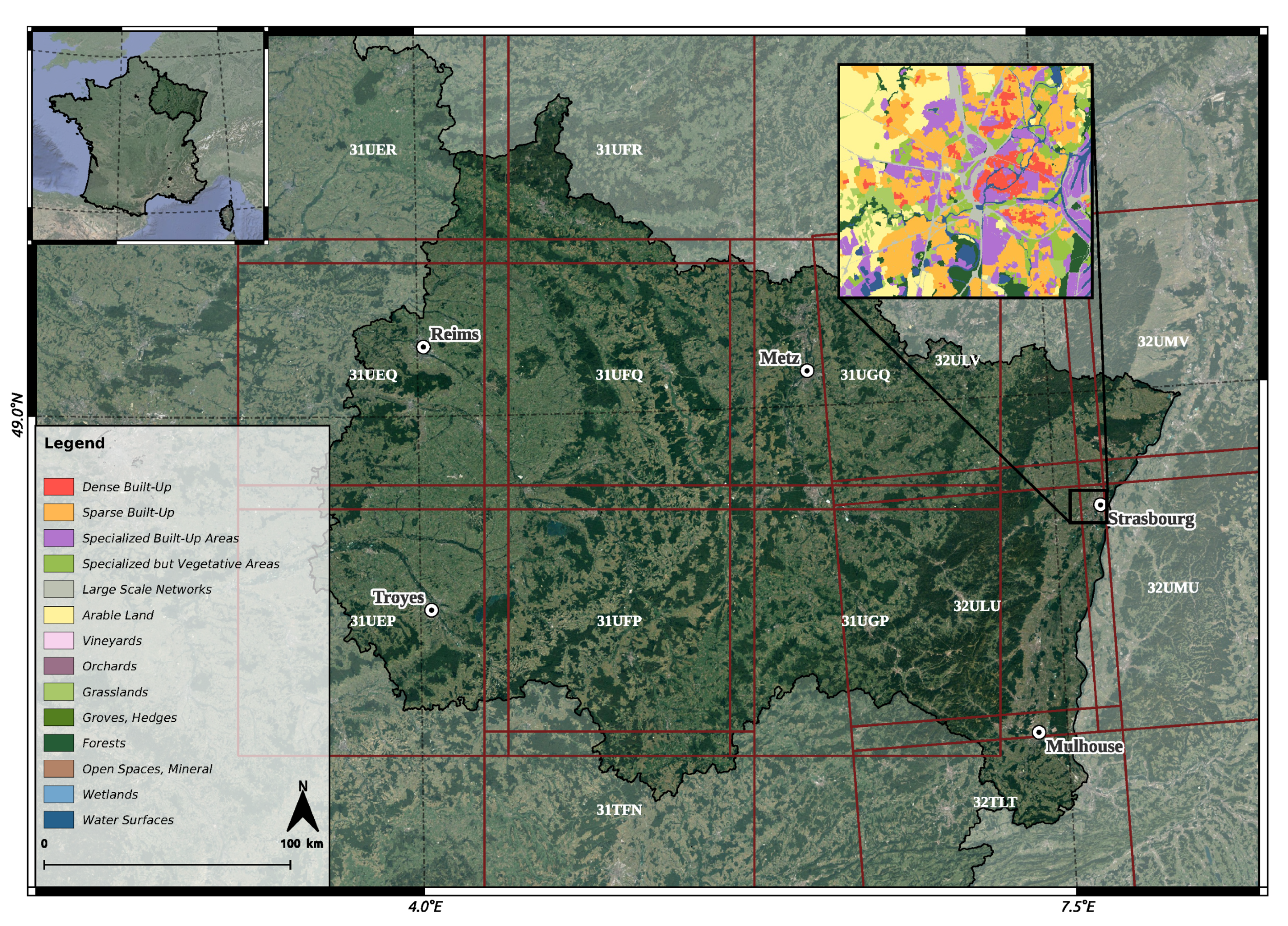
Figure 1. Grand-Est region with ground reference subset, Sentinel-2 tiling grid and major cities.
Remotesensing 15 00151 g001
Figure 2. Number of patches with at least one Sentinel-2 image associated per month.
Remotesensing 15 00151 g002
Figure 3. Distribution of patches over the study area according to the number of days between two consecutive dates for the months of July, August, September and November (2020).
Remotesensing 15 00151 g003
Figure 4. Train, validation and test sets for the selected multitemporal and multimodal patches.
Remotesensing 15 00151 g004
Figure 5. Sentinel-1 and Sentinel-2 ConvLSTM+Inception method ( | | sign means concatenate). Inception module has been added and the U-Net netwrok take as input the concatenation of the 2 ConvLSTM and the Inception module. This network is used for ConvLSTM and ConvLSTM+Inception methods.
Remotesensing 15 00151 g005
Figure 6. ConvLSTM structure.
Remotesensing 15 00151 g006
Figure 7. Naive Inception module.
Remotesensing 15 00151 g007
Figure 8. Results for each method for 6 semantic classes (Legend is available in Table 3).
Remotesensing 15 00151 g008
Figure 9. Results for each method for 6 semantic classes (Legend is available in Table 3).
Remotesensing 15 00151 g009
Figure 10. Scatter plot to compare UFs (classes 1 to 5 in Table 3) classifications of ConvLSTM+ Inception-S1S2 for 10 classes between every method implemented for 6 classes. (a) 10 classes ConvLSTM+Inception-S1S2 vs. 6 classes ConvLSTM-S1. (b) 10 classes ConvLSTM+Inception-S1S2 vs. 6 classes ConvLSTM-S2. (c) 10 classes ConvLSTM+Inception-S1S2 vs. 6 classes ConvLSTM-S1S2. (d) 10 classes ConvLSTM+Inception-S1S2 vs. 6 classes ConvLSTM+Inception-S1S2.
Remotesensing 15 00151 g010aRemotesensing 15 00151 g010b
Table 1. Number of patches depending on the days gap for two consecutive months.
Days Gap for Two Consecutive MonthsNumber of Patches
156560
165890
175890
184960
193178
203178
Table 2. Semantic classes distribution for MultiSenGE dataset.
MultiSenGE Semantic ClassesMultiSenGE Distribution
Dense Built-Up (1)0.37%
Sparse Built-Up (2)3.64%
Specialized Built-Up Areas (3)2.17%
Specialized but Vegetative Areas (4)0.44%
Large Scale Networks (5)0.91%
Arable Lands (6)38.73%
Vineyards (7)0.98%
Orchards (8)0.15%
Grasslands (9)18.87%
Groves, Hedges (10)0.01%
Forests (11)32.52%
Open Spaces, Mineral (12)0.01%
Wetlands (13)0.31%
Water Surfaces (14)0.89%
Table 3. Semantic classes for MultiSenGE dataset and our reclassification in 6 and 10 classes.
MultiSenGE Semantic Classes10 Classes6 Classes
Dense Built-Up (1)Dense Built-Up (1)Dense Built-Up (1)
Sparse Built-Up (2)Sparse Built-Up (2)Sparse Built-Up (2)
Specialized Built-Up Areas (3)Specialized Built-Up Areas (3)Specialized Built-Up Areas (3)
Specialized but Vegetative Areas (4)Specialized but Vegetative Areas (4)Specialized but Vegetative Areas (4)
Large Scale Networks (5)Large Scale Networks (5)Large Scale Networks (5)
Arable Lands (6)Arable Lands (6)Non-urban areas (6)
Vineyards (7)Vineyards and Orchards (7)
Orchards (8)
Grasslands (9)Grasslands (8)
Groces, Hedges (10)Forests and
semi-natural areas (9)
Forests (11)
Open Spaces, Mineral (12)
Wetlands (13)Water Surfaces (10)
Water Surfaces (14)
Table 4. List of experiments based on the methods presented.
NameSensorsMethodNumber of Classes
ConvLSTM-S1Sentinel-1ConvLSTM6 classes
ConvLSTM-S2Sentinel-2ConvLSTM6 classes
ConvLSTM-S1S2Sentinel-1 and Sentinel-2ConvLSTM6 classes
ConvLSTM-S1Sentinel-1ConvLSTM10 classes
ConvLSTM-S2Sentinel-2ConvLSTM10 classes
ConvLSTM-S1S2Sentinel-1 and Sentinel-2ConvLSTM10 classes
ConvLSTM+Inception-S1S2Sentinel-1 and Sentinel-2ConvLSTM and Inception6 classes
ConvLSTM+Inception-S1S2Sentinel-1 and Sentinel-2ConvLSTM and Inception10 classes
Table 5. Results of all methods for the test zone located in the north of Strasbourg, Grand-Est, France (In bold the higher value for each metric and for each method).
ConvLSTM-S1ConvLSTM-S2
PrecisionRecallF1PrecisionRecallF1
Class 10.13350.93970.23370.25790.87040.3980
Class 20.44760.38090.41160.55750.72680.6310
Class 30.35600.58130.44160.31000.77630.4431
Class 40.07750.50720.13440.05280.48580.0953
Class 50.13130.55160.21220.21370.79950.3372
Class 60.99370.89370.94100.99790.86630.9274
W-Avg0.94690.86610.90010.95440.85740.8958
ConvLSTM-S1S2ConvLSTM+Inception-S1S2
PrecisionRecallF1PrecisionRecallF1
Class 10.31220.76240.44300.23080.85990.3639
Class 20.56710.77060.65330.62600.64720.6364
Class 30.46540.68590.55450.47940.76470.5894
Class 40.03140.57390.05950.03120.44610.0584
Class 50.27450.80850.40990.27360.78980.4064
Class 60.99710.84460.91450.99650.87190.9301
W-Avg0.95780.83690.88750.95910.85960.9018
Table 6. Cohen’s Kappa for each method for 6 semantic classes (In bold the best method).
MethodCohen’s Kappa
ConvLSTM-S10.3929
ConvLSTM-S20.4223
ConvLSTM-S1S20.3852
ConvLSTM+Inception-S1S20.4186
Table 7. Results of all methods for the test zone located in the west of the Grand-Est region (In bold the higher value for each metric and for each method).
ConvLSTM-S1ConvLSTM-S2
PrecisionRecallF1PrecisionRecallF1
Class 10.18720.92470.31140.56290.49680.5278
Class 20.57180.52240.54600.68140.76250.7197
Class 30.42080.64800.51030.49090.73290.5880
Class 40.08920.49730.15120.15970.34990.2193
Class 50.21420.61830.31820.29140.80760.4283
Class 60.96490.85400.90600.98380.92630.9542
Class 70.83610.56250.67260.90030.87370.8868
Class 80.38900.41110.39970.57200.43360.4933
Class 90.75150.82800.78790.90020.76970.8299
Class 100.31430.47480.37820.16110.91060.2737
W-Avg0.84220.78360.80550.90000.85170.8696
ConvLSTM-S1S2ConvLSTM+Inception-S1S2
PrecisionRecallF1PrecisionRecallF1
Class 10.27360.81990.41030.38700.71900.5031
Class 20.64980.72870.68700.66720.80660.7303
Class 30.58400.39550.47160.46120.76320.5749
Class 40.18850.26920.22170.18630.36430.2465
Class 50.27390.86660.41630.42900.75600.5474
Class 60.98620.90330.94300.97180.95580.9637
Class 70.78220.92030.84570.88690.85120.8687
Class 80.49140.45550.47280.74220.39490.5155
Class 90.85160.85330.85240.85850.86430.8614
Class 100.27590.86600.41850.46540.70740.5614
W-Avg0.88250.84820.86000.89770.88310.8851
Table 8. Cohen’s Kappa for each method for 10 semantic classes (In bold the best method).
MethodCohen’s Kappa
ConvLSTM-S10.6422
ConvLSTM-S20.7445
ConvLSTM-S1S20.7482
ConvLSTM+Inception-S1S20.7945
Disclaimer/Publisher’s Note: The statements, opinions and data contained in all publications are solely those of the individual author(s) and contributor(s) and not of MDPI and/or the editor(s). MDPI and/or the editor(s) disclaim responsibility for any injury to people or property resulting from any ideas, methods, instructions or products referred to in the content.