Abstract
The Baltic Sea is one of the fastest-warming marginal seas globally, and its temperature rise has adversely affected its physical and biochemical characteristics. In this study, forty years (1982–2021) of sea surface temperature (SST) data from the advanced very high resolution radiometer (AVHRR) were used to investigate spatial and temporal SST variability of the Baltic Sea. To this end, annual maximum and minimum SST stacked series, i.e., time series of stacked layers of satellite data, were generated using high-quality observations acquired at night and were fed to an automatic algorithm to detect linear and non-linear trend patterns. The linear trend pattern was the dominant trend type in both stacked series, while more pixels with non-linear trend patterns were detected when using the annual minimum SST. However, both stacked series showed increases in SST across the Baltic Sea. Annual maximum SST increased by an average of 0.062 ± 0.041 °C per year between 1982 and 2021, while annual minimum SST increased by an average of 0.035 ± 0.017 °C per year over the same period. Averaging annual maximum and minimum trends produces a spatial average of 0.048 ± 0.022 °C rise in SST per year over the last four decades.
1. Introduction
Sea surface temperature (SST) has been recognized as an essential climate variable and one of the leading indicators of climate change [1]. SST is a necessary parameter for atmospheric models, atmosphere–ocean interaction studies, and ocean forecasting from regional to global scales [2,3]. Information about SST conditions at local to regional scales is required to understand marine ecosystem dynamics [4] and the direct and indirect effects of climate change on fish stocks [5]. These reasons justify the necessity of measuring high-quality SST through time, supporting the successful accomplishment of relevant studies, and monitoring SST dynamics. Satellite remote sensing observations offer a unique opportunity to measure SST in consistent spatial and temporal scales [6,7]. The extensive spatial coverage and long temporal record of satellite observations provide a synoptic view of SST and enable the monitoring of their dynamics. Accordingly, several global and regional SST datasets based on remote sensing satellites have been generated [2,8,9], which could be used to quantify the spatial and temporal dynamics of SST.
The Baltic Sea is one of the fastest-warming marginal seas [10], and its SST variability has attracted the interest of researchers. Several recent studies have been conducted based on either remote sensing SST observations or other sources (e.g., atmospheric forcing models) to quantify the magnitude of SST dynamics through time [2,10,11,12,13,14,15]. These studies are in general agreement that the Baltic SST trend has been increasing, though the reported magnitudes differ mainly due to different data sources or studied periods. For instance, Stramska and Bialogrodzka [15] examined the spatial and temporal SST variability of the Baltic Sea using 31 years (1982–2013) of the advanced very high resolution radiometer (AVHRR) observations and reported increasing trends ranging between 0.03 °C and 0.06 °C per year. Likewise, Høyer and Karagali [2] used AVHRR observations to determine linear temporal SST dynamics of the Baltic Sea between 1982 and 2012, which were reported to be 0.04 °C per year. More recently, Kniebusch et al. [13] investigated the Baltic Sea SST variations using reconstructed atmospheric forcing field data. Their results revealed increasing SST trends in the Baltic Sea between 1856 and 2005, with average magnitudes between 0.03 °C and 0.06 °C per decade in northeastern and southwestern regions, respectively. Furthermore, they found that an intensified increase in SST occurred in later decades, reaching 0.4 °C per decade between 1978 and 2007. Likewise, Dutheil et al. [10] used similar data to those of Kniebusch et al. [13] for the period 1850–2008 to analyze the spatial and temporal SST trends in the Baltic Sea. Their results indicated a mean SST increase of 0.047 °C per decade with a standard deviation (0.008 °C per decade).
Climate change increases SST and alters ocean circulation patterns [16], and the warming of the Baltic Sea has resulted in critical physical and biochemical effects that have direct effects on marine ecosystem functioning and ecosystem services. Likewise, the increase in the melting rate of sea ice due to SST rise is also reported to cause environmental issues [17]. These include catalyzing eutrophication, enriching cyanobacteria blooms, and increasing hypoxia [18,19], which negatively affect the ecosystem services provided by the Baltic Sea, such as fisheries and tourism. As the Baltic is likely to continue warming in the future [20], timely monitoring of its SST is necessary to support efficient marine ecosystem management. Although several studies were conducted to investigate the SST trend in the Baltic Sea, there has been a considerable paucity of studies that have included Baltic SST observations from the current decade (2011–2021), which is surprising since this decade is the warmest on record according to the Copernicus Climate Change Service [21]. More notably, previous studies based on satellite observations have only considered linear trend patterns, while SST could have non-linear dynamics due to the non-linear impact of climate change and climate feedback [10]. Therefore, the main objective of this paper is to detect both linear and non-linear trend patterns of SST in the Baltic Sea based on four decades (1982–2021) of AVHRR satellite observations using an automatic polynomial trend analysis framework, PolyTrend [22], and generate per-pixel slope magnitude, along with the t-test analysis for statistical significance evaluation, to better understand Baltic Sea SST dynamics. Finally, the slope magnitudes were separately computed for five subregions in the Baltic Sea.
2. Study Area
The study area is in northern Europe between 53°57′N and 65°46′N longitudes and between 8°34′E and 29°50′E latitudes (see Figure 1). It includes mainly the Baltic Sea (i.e., Gulf of Bothnia, Gulf of Finland, Gulf Riga, and Baltic Sea), Kattegat, and part of Skagerrak. The Baltic Sea is connected to the North Sea and the Atlantic Ocean through the narrow straits of Denmark. As the Baltic Sea is semi-closed and receives a considerable inflow of freshwater from surrounding rivers, its waters are brackish with salinity varying between 3 and 12 g/kg [23]. It has high bathymetric variability with a relatively low average depth of approximately 54 m [10]. The Baltic Sea has been recognized as one of the fastest-warming marginal seas in recent decades, which has had adverse effects on its biochemical and physical conditions [10]. Figure 1 presents the spatial patterns of maximum SST values over the study area in 2021 and 1982, which were 20.89 °C and 19.29 °C on average, respectively, possibly an indication of a warming condition. The per-pixel maximum SST values for 2021 and 1982 were obtained by computing the maximum SST value of each pixel using all available high-quality AVHRR SST observations within the corresponding year, acquired at night (see Section 3.1). Finally, spatial averages of all maximum SST values were computed to be reported as a single indicator.
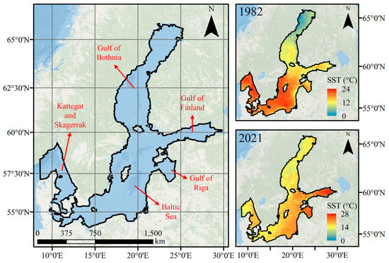
Figure 1.
The geographical location of the study area, along with maximum sea surface temperature (SST) in 1982 and 2021 computed using high-quality AVHRR remote sensing data acquired at night.
3. Materials and Methods
3.1. Sea Surface Temperature (SST) Dataset
The AVHRR Pathfinder Version 5.3 (PFV5.3) SST dataset was used for trend analysis in this study. PFV5.3 is the latest release of the Pathfinder SST program, providing a long-term global SST dataset for research, modeling, and trend analysis [24]. PFV5.3 is generated from a combination of AVHRR sensors onboard the National Oceanic and Atmospheric Administration (NOAA) satellite series. It contains day and night observations (i.e., twice daily) of global SST values at 4 km spatial resolution from August 1981 to the present. The SST values have been computed through a non-linear SST algorithm [25], in which the corresponding coefficients have been determined using co-located in situ and satellite measurements [26]. The PFV5.3 dataset provides SST values with reasonable accuracy with a root mean square error (RMSE) in the range of 0.31 °C to 0.37 °C [27].
The PFV5.3 SST dataset was downloaded and pre-processed using the Google Earth Engine (GEE) cloud computing platform [28,29], which is available through the GEE Snippet of ee.ImageCollection(“NOAA/CDR/SST_PATHFINDER/V53”). The AVHRR PFV5.3 provides day and night global SST observations. Here, only night SST observations (i.e., one per night) were used to ultimately generate two forty-year stacked series for trend analysis. This is rooted in the fact that day observations are subjected to the diurnal warming effect, which is reported to be significant in the Baltic Sea [30].
Night-time SST values were first separated for further processing. The quality flag data were then incorporated to exclude lower-quality SST values. Only SST values with quality flags equal to 4 (acceptable quality) and 5 (best quality) were used for further analysis. In the final step, annual maximum and minimum values for each year between 1982 and 2021 were computed using high-quality SST values acquired at night. This resulted in two spatial time series that included forty SST values, one for each year, covering the last forty years (1982–2021). Although maximum and minimum functions were used here to generate the two SST stacked series for trend analysis, in other studies [31,32], average SST values in each year were considered. However, it was not possible to use annual average SST values in this study because the number and temporal distribution (i.e., positions of observations in a year) of high-quality SST observations for all pixels were not identical over the Baltic Sea. Therefore, averaging could lead to an inconsistent dataset that would introduce further uncertainties into the trend analysis.
3.2. Trend Analysis Method
The PolyTrend algorithm [22] was implemented to examine SST trends of the study area over the last four decades. This algorithm was originally developed for automatic vegetation trend analysis [22] and was later applied to other disciplines, such as precipitation [32], tropospheric NO2 [33], and air temperature trend analyses [34]. The PolyTrend algorithm detects linear and non-linear trends and considers five different trend patterns, as shown in Figure 2. The algorithm begins by checking the existence of a cubic trend, and if the required criteria are not met, it will proceed with checking the existence of a quadratic trend. If the criteria of either cubic or quadratic trend patterns are met but the SST net change between the start and end year of the study period is negligible (i.e., statistically insignificant), then a concealed trend will be assigned. This is determined by checking the significance of the coefficient of a linear fit. In case of rejecting the existence of a non-linear trend pattern, a linear function is fitted to the input data, and the significance of the linear coefficient will lead to the assignment of the linear trend pattern. Finally, the no-trend pattern will be assigned to the corresponding input data when no statistically significant trend (linear or non-linear) is found. It is important to note that the algorithm can be employed with tunable confidence intervals based on the Student’s t-test, which in this study was set to 95%.
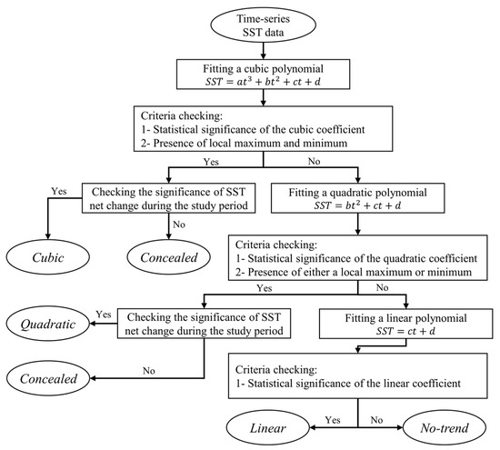
Figure 2.
Flowchart of the PolyTrend algorithm implemented to examine the sea surface temperature (SST) trend of the Baltic Sea (after Jamali et al. [22]).
Accordingly, the two forty-year SST stacked series were fed to the PolyTrend algorithm, and each pixel containing 40 SST values (either annual maximum or minimum) was subjected to trend analysis, according to Figure 2. Then, per-pixel trend patterns, SST variability, and slope magnitude maps were produced based on annual maximum and minimum SST. Finally, for each stacked series, SST variability and slope magnitude were averaged to generate representative maps that contain the results of both annual maximum and minimum SST.
4. Results
The per-pixel SST trend pattern between 1982 and 2021 for approximately 47,000 pixels that comprise the Baltic Sea is shown in Figure 3. The linear trend pattern was the dominant trend type detected by the PolyTrend algorithm when using annual maximum SST (Figure 3a). Areas with direct exchange with the North Sea, such as the western parts of the Baltic Sea and Skagerrak, were dominated by the no-trend patterns. Meanwhile, non-linear trend patterns (i.e., cubic, quadratic, and concealed) were only detected nearshore. The non-linearity of trends in nearshore areas could possibly be due to water–land interactions, water level effects on SST values in each year, and influence of land surface warming/cooling on adjacent water surfaces in remote sensing data. Annual maximum and annual minimum Baltic Sea SST exhibited markedly different behavior over the course of the study period. Annual maximum SST exhibited a linear trend pattern over 81.01% of the pixels comprising the Baltic Sea. The remainder exhibited no-trend, quadratic, concealed, and cubic trends representing 15.33%, 1.42%, 1.32%, and 0.93% of pixels, respectively (Figure 3a). On the other hand, annual minimum SST had a more heterogeneous pattern, with non-linear trend patterns being more frequent (Figure 3b). Although the two dominant trend patterns for annual minimum SST were linear (39.86%) and no-trend (28.65%), the portion of non-linear trends was higher than annual maximum SST. In particular, the pixels that were assigned to cubic, concealed, and quadratic trend patterns covered 19.71%, 8.86%, and 2.94% of the surface area, respectively. Despite the differences in trend pattern, both annual maximum and minimum stacked series showcase the rise in Baltic SST based on the detected trend directions. In fact, nearly 97% of pixels in both stacked series had a positive trend direction over the last forty years. Meanwhile, a low number of pixels were found to have negative trends, which were located nearshore. This discrepancy could be due to uncertainties associated with pixels near land, as mentioned earlier.
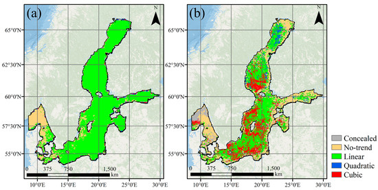
Figure 3.
Sea surface temperature (SST) trend maps of the Baltic Sea over the last four decades derived using (a) annual maximum and (b) annual minimum SST values of AVHRR Pathfinder data acquired at night.
The temporal variability of annual maximum and minimum SST across the Baltic Sea is shown by the standard deviation (SD) over the last forty years (Figure 4). The SD of annual maximum SST ranged between 1.4 °C and 7.3 °C (Figure 4a), and that of annual minimum SST was between 0.5 °C and 7.1 °C (Figure 4b). For annual maximum and annual minimum SST, 95% of pixels had SD values lower than 2.7 °C and 2.4 °C, respectively. For both stacked series, pixels with very high SD values were mainly located nearshore. Considering the spatial average of annual maximum and minimum SST (Figure 4c), the SD values had an average of 1.75 ± 0.44 °C over the last four decades, indicating relatively high variation across the Baltic.
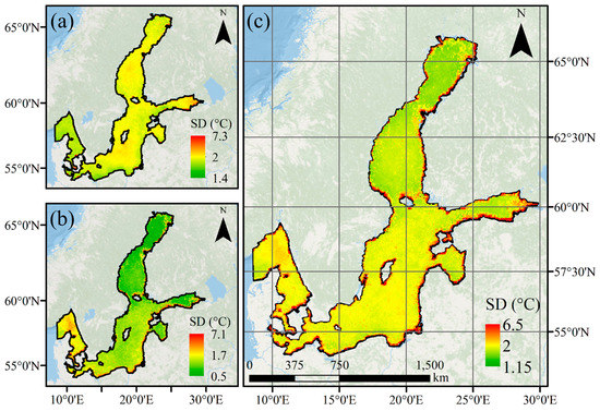
Figure 4.
Standard deviation (SD) of AVHRR Pathfinder sea surface temperature (SST) of the Baltic Sea over the last four decades based on (a) annual maximum SST, (b) annual minimum SST, and their spatial average (c) acquired at night.
Finally, the slope magnitudes of SST changes over the past forty years were calculated based on annual maximum and minimum stacked series (Figure 5). Figure 5a illustrates the spatial distribution of the slope of annual maximum SST ranging between −0.35 °C and 0.23 °C per year, with an average of 0.062 ± 0.041 °C per year. The western parts of the Baltic Sea and Skagerrak had relatively lower slope magnitudes, while the northern parts (latitudes > 60° N) had higher slope magnitudes than the southern ones. Likewise, Figure 4b shows the SST slope magnitudes calculated based on annual minimum SST, varying from −0.11 °C to 0.34 °C per year, with an average of 0.035 ± 0.017 °C per year. In contrast to annual maximum SST (Figure 5a), southern parts (latitudes < 60° N) of the Baltic Sea experienced a relatively higher rate of annual minimum SST rise (Figure 5b). The statistical analysis revealed that 16.65% and 37.51% of pixels had insignificant trends in annual maximum and minimum SST, respectively. Figure 5c,d show uncertainties of slope estimation for both SST. In general, larger uncertainties were observed in the southern parts of the study area, while more significant uncertainties were observed in the Kattegat and Skagerrak according to annual minimum SST. The average slope of annual maximum and minimum SST (Figure 5e) represents a relatively similar warming pattern across the Baltic Sea, except for the western parts with lower warming rates in the Skagerrak, which could be due to the direct water exchange with the North Sea and the Atlantic Ocean. The magnitude of the average annual maximum and minimum SST slopes varied from −0.18 °C to 0.19 °C per year, with a spatial average of 0.048 ± 0.022 °C per year across the Baltic (Figure 5e).
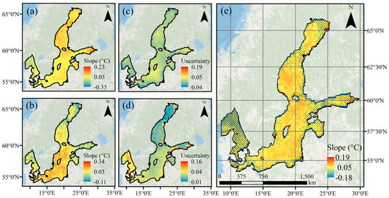
Figure 5.
AVHRR Pathfinder sea surface temperature (SST) change slope magnitudes and associated uncertainties across the Baltic Sea over the last four decades calculated using (a,c) annual maximum, (b,d) annual minimum, and (e) the average slope magnitudes of both SST stacked series. Insignificant trends based on annual maximum and minimum SST are hatched with black lines at 45 and 135 degrees, respectively.
The slope magnitudes were also computed for five different subregions of the study area that could be of interest to local researchers. According to the maximum/minimum stacked series, the average SST change slopes of the Gulf of Bothnia, Gulf of Finland, Gulf of Riga, Baltic Sea (only southern parts), and Kattegat and Skagerrak were 0.076/0.029 °C, 0.052/0.020 °C, 0.060/0.030 °C, 0.062/0.043 °C, and 0.038/0.029 °C, respectively. The average slope of annual maximum and minimum SST (Figure 5c) indicated 0.052 ± 0.018 °C, 0.036 ± 0.041 °C, 0.045 ± 0.031 °C, 0.052 ± 0.018 °C, and 0.033 ± 0.019 °C annual SST rise for the Gulf of Bothnia, Gulf of Finland, Gulf of Riga, Baltic Sea (only southern parts), and Kattegat and Skagerrak, on average, and the slope magnitudes were in ranges of −0.17 °C to 0.19 °C. This reveals that the Baltic Sea and Gulf of Bothnia experienced higher SST rise, while the Kattegat and Skagerrak had the lowest SST rise over the past four decades.
Less than 3.2% of spatially averaged pixels had negative or high positive slope magnitudes greater than 0.09 °C per year (Table 1), and these were mainly located nearshore. Furthermore, the highest portion of pixels for annual maximum SST (63%), annual minimum SST (61.4%), and their spatial average (75.9%) had SST slopes from 0.06 °C to 0.09 °C, 0.03 °C to 0.06 °C, and 0.03 °C to 0.06 °C per year, respectively, demonstrating considerable SST rise across the Baltic Sea.

Table 1.
The proportion (%) of different slope magnitude ranges of the Baltic Sea surface temperature (SST) based on annual maximum SST, annual minimum SST, and their average values over the last four decades.
5. Discussion
The trend analysis results demonstrated a spatially consistent SST rise across the Baltic Sea in recent decades, which is in agreement with previous studies [2,10,11,12,13,14,15]. Stramska and Białogrodzka [15] estimated the slope magnitudes to be in the range of 0.03 °C and 0.06 °C per year for their study period (1982–2013). In this study, 75.9% of pixels had the same range based on the averaged slope values of annual maximum and minimum SST (see Table 2). The spatially averaged slope value of this study was 0.048 °C per year, which is close to the value of 0.041 °C per year for the years 1982 to 2012 reported by Høyer and Karagali [2].
The PFV5.3 SST observations were collected by AVHRR sensors onboard the NOAA satellite series (e.g., NOAA-7, -7, 9, 11, 14, 16, 17, 18, and 19). These platforms do not have identical orbits, and thus, the local time of SST observations may differ between years depending on the platforms. This common issue in long-term datasets could affect the trend analysis results. However, the AVHRR PFV5.3 has been generated according to the Group for High Resolution SST (GHRSST) data specification and reported to be suitable for long-term trend analysis [24].
In this study, only high-quality SST observations collected at night were used for trend analysis to eliminate the effect of diurnal warming in daytime observations [2], which was reported to be significant in the Baltic Sea [30]. Since satellite local time overpasses are not identical (e.g., due to satellite drifts, different missions, and climatic conditions), the SST observations collected in the daytime are subjected to different diurnal warming effects, which can reach up to 7 °C under low wind and strong solar illumination [35]. This issue associated with diurnal warming will introduce spurious interannual trends and can reduce the robustness of annual trend analysis results [8].
It was anticipated that annual maximum SST would lead to a higher SST slope magnitude than annual minimum SST [36]. However, the results paint a complex picture of the SST trend in the Baltic over the past four decades. Annual maximum SST has been increasing faster (i.e., higher slope values) in the northern Baltic Sea, i.e., the Gulf of Bothnia and the Gulf of Finland, than in the southern parts (Figure 4a). This trend pattern was also found by Siegel, Gerth, and Tschersich [37] and Lehmann, Getzlaff, and Harlaß [38] but for shorter time periods (1990–2004 and 1990–2008, respectively). The likely cause for this faster trend is the result of increases in summer warming [38], and the fact that both the Gulfs of Bothnia and Finland are surrounded by land, which causes water temperatures in these parts of the Baltic Sea to be under the influence of the relatively faster warming land [2]. Future projections of temperature indicate a significant increase in the northern and northeastern portion of the Baltic Sea by the end of the 21st century, which is driven by disappearance of the sea ice [10].
A considerably high proportion (81.01%) of the trend in annual maximum SST was linear. This is expected because annual maximum SST coincides with the northern summer warming [15], which has been experiencing more frequent strong heatwaves [39,40,41]. However, this intense warming in recent years has had a different effect on annual minimum SST in the Baltic Sea, which coincides with northern winter cooling. Annual minimum SST has double the non-linear trends and half the linear trends. Approximately one-third (31.51%) of the trends in annual minimum SST are non-linear and are evenly distributed across the Baltic Sea. Annual minimum SST is affected by the extent of sea ice, but there are many associated feedback loops, such as surface winds, upwelling, and the isolation of the water from the atmosphere [10], which can potentially contribute to the non-linearity of the trend.
6. Conclusions
This study used forty years of AVHRR satellite observations across the Baltic Sea and found a consistent rise in SST during that period. Only high-quality SST observations acquired at night were considered to eliminate the diurnal warming effect. The results show that the trend patterns largely depended on whether annual maximum or annual minimum SST was considered. The trend pattern detection with annual minimum SST stacked series obtained more non-linear trend patterns (31.51%), while the non-linear trend patterns were scarcely detected when using annual maximum SST.
Furthermore, annual maximum SST led to a higher SST slope estimate (on average 0.062 ± 0.041 °C per year) than annual minimum SST (on average 0.035 ± 0.017 °C per year). Accordingly, to provide a moderate estimate of the SST rise, the generated slope maps were averaged, leading to an estimation of about 0.048 ± 0.022 °C per year, which is generally in agreement with previous studies.
Author Contributions
Conceptualization, S.J. and A.G.; methodology, S.J. and A.G.; software, S.J. and A.G.; validation, S.J. and A.G.; formal analysis, S.J. and A.G.; investigation, S.J., A.G. and A.M.A.; resources, S.J.; data curation, A.G.; writing—original draft preparation, S.J. and A.G.; writing—review and editing, S.J., A.G. and A.M.A.; visualization, A.G.; supervision, S.J.; project administration, S.J. All authors have read and agreed to the published version of the manuscript.
Funding
This research received no external funding.
Data Availability Statement
The sea surface temperature dataset supporting the reported results of this paper is publicly available in the Google Earth Engine data catalog.
Acknowledgments
During this study, Arsalan Ghorbanian was funded by Erasmus + ICM programme for a 5-month stay at Lund University, Sweden, and thanks the European Union.
Conflicts of Interest
The authors declare no conflict of interest.
References
- Bojinski, S.; Verstraete, M.; Peterson, T.C.; Richter, C.; Simmons, A.; Zemp, M. The Concept of Essential Climate Variables in Support of Climate Research, Applications, and Policy. Bull. Am. Meteorol. Soc. 2014, 95, 1431–1443. [Google Scholar] [CrossRef]
- Høyer, J.L.; Karagali, I. Sea Surface Temperature Climate Data Record for the North Sea and Baltic Sea. J. Clim. 2016, 29, 2529–2541. [Google Scholar] [CrossRef]
- Hollmann, R.; Merchant, C.J.; Saunders, R.; Downy, C.; Buchwitz, M.; Cazenave, A.; Chuvieco, E.; Defourny, P.; de Leeuw, G.; Forsberg, R.; et al. The ESA Climate Change Initiative: Satellite Data Records for Essential Climate Variables. Bull. Am. Meteorol. Soc. 2013, 94, 1541–1552. [Google Scholar] [CrossRef]
- Kim, G.-U.; Seo, K.-H.; Chen, D. Climate Change over the Mediterranean and Current Destruction of Marine Ecosystem. Sci. Rep. 2019, 9, 18813. [Google Scholar] [CrossRef] [PubMed]
- Gamito, R.; Teixeira, C.M.; Costa, M.J.; Cabral, H.N. Are Regional Fisheries’ Catches Changing with Climate? Fish. Res. 2015, 161, 207–216. [Google Scholar] [CrossRef]
- Sobrino, J.A.; García-Monteiro, S.; Julien, Y. Surface Temperature of the Planet Earth from Satellite Data over the Period 2003–2019. Remote Sens. 2020, 12, 2036. [Google Scholar] [CrossRef]
- Amani, M.; Ghorbanian, A.; Asgarimehr, M.; Yekkehkhany, B.; Moghimi, A.; Jin, S.; Naboureh, A.; Mohseni, F.; Mahdavi, S.; Layegh, N.F. Remote Sensing Systems for Ocean: A Review (Part 1: Passive Systems). IEEE J. Sel. Top. Appl. Earth Obs. Remote Sens. 2021, 15, 210–234. [Google Scholar] [CrossRef]
- Merchant, C.J.; Embury, O.; Bulgin, C.E.; Block, T.; Corlett, G.K.; Fiedler, E.; Good, S.A.; Mittaz, J.; Rayner, N.A.; Berry, D.; et al. Satellite-based time-series of sea-surface temperature since 1981 for climate applications. Sci. Data 2019, 6, 223. [Google Scholar] [CrossRef]
- O’Carroll, A.G.; Armstrong, E.M.; Beggs, H.M.; Bouali, M.; Casey, K.S.; Corlett, G.K.; Dash, P.; Donlon, C.J.; Gentemann, C.L.; Høyer, J.L.; et al. Observational Needs of Sea Surface Temperature. Front. Mar. Sci. 2019, 6, 420. [Google Scholar] [CrossRef]
- Dutheil, C.; Meier, H.E.M.; Gröger, M.; Börgel, F. Understanding Past and Future Sea Surface Temperature Trends in the Baltic Sea. Clim. Dyn. 2021, 58, 3021–3039. [Google Scholar] [CrossRef]
- Meier, H.E.; Dieterich, C.; Gröger, M.; Dutheil, C.; Börgel, F.; Safonova, K.; Christensen, O.B.; Kjellström, E. Oceanographic Regional Climate Projections for the Baltic Sea until 2100. Earth Syst. Dyn. 2022, 13, 159–199. [Google Scholar] [CrossRef]
- Bradtke, K. Landsat 8 Data as a Source of High Resolution Sea Surface Temperature Maps in the Baltic Sea. Remote Sens. 2021, 13, 4619. [Google Scholar] [CrossRef]
- Kniebusch, M.; Meier, H.E.M.; Neumann, T.; Börgel, F. Temperature variability of the baltic sea since 1850 and attribution to atmospheric forcing variables. J. Geophys. Res. Ocean. 2019, 124, 4168–4187. [Google Scholar] [CrossRef]
- Liu, Y.; Fu, W. Assimilating High-Resolution Sea Surface Temperature Data Improves the Ocean Forecast Potential in the Baltic Sea. Ocean Sci. 2018, 14, 525–541. [Google Scholar] [CrossRef]
- Stramska, M.; Białogrodzka, J. Spatial and Temporal Variability of Sea Surface Temperature in the Baltic Sea Based on 32-Years (1982–2013) of Satellite Data. Oceanologia 2015, 57, 223–235. [Google Scholar] [CrossRef]
- Winton, M.; Griffies, S.M.; Samuels, B.L.; Sarmiento, J.L.; Frölicher, T.L. Connecting Changing Ocean Circulation with Changing Climate. J. Clim. 2013, 26, 2268–2278. [Google Scholar] [CrossRef]
- Pärn, O.; Friedland, R.; Rjazin, J.; Stips, A. Regime Shift in Sea-Ice Characteristics and Impact on the Spring Bloom in the Baltic Sea. Oceanologia 2022, 64, 312–326. [Google Scholar] [CrossRef]
- Viitasalo, M.; Bonsdorff, E. Global Climate Change and the Baltic Sea Ecosystem: Direct and Indirect Effects on Species, Communities and Ecosystem Functioning. Earth Syst. Dyn. 2022, 13, 711–747. [Google Scholar] [CrossRef]
- Zillén, L.; Conley, D.J.; Andrén, T.; Andrén, E.; Björck, S. Past Occurrences of Hypoxia in the Baltic Sea and the Role of Climate Variability, Environmental Change and Human Impact. Earth-Sci. Rev. 2008, 91, 77–92. [Google Scholar] [CrossRef]
- Gröger, M.; Arneborg, L.; Dieterich, C.; Höglund, A.; Meier, H.E.M. Summer Hydrographic Changes in the Baltic Sea, Kattegat and Skagerrak Projected in an Ensemble of Climate Scenarios Downscaled with a Coupled Regional Ocean–Sea Ice–Atmosphere Model. Clim. Dyn. 2019, 53, 5945–5966. [Google Scholar] [CrossRef]
- Copernicus Climate Change Service 2020 Warmest Year on Record for Europe; Globally, 2020 Ties with 2016 for Warmest Year Recorded. Available online: https://climate.copernicus.eu/copernicus-2020-warmest-year-record-europe-globally-2020-ties-2016-warmest-year-recorded#:~:text=The%20Copernicus%20Climate%20Change%20Service%20(C3S)%20today%20reveals%20that%20globally,2020%20the%20warmest%20decade%20recorded (accessed on 20 December 2022).
- Jamali, S.; Seaquist, J.; Eklundh, L.; Ardö, J. Automated Mapping of Vegetation Trends with Polynomials Using NDVI Imagery over the Sahel. Remote Sens. Environ. 2014, 141, 79–89. [Google Scholar] [CrossRef]
- Fonselius, S.; Valderrama, J. One Hundred Years of Hydrographic Measurements in the Baltic Sea. J. Sea Res. 2003, 49, 229–241. [Google Scholar] [CrossRef]
- Casey, K.S.; Brandon, T.B.; Cornillon, P.; Evans, R. The Past, Present, and Future of the AVHRR Pathfinder SST Program. In Oceanography from Space: Revisited; Barale, V., Gower, J.F.R., Alberotanza, L., Eds.; Springer: Dordrecht, The Netherlands, 2010; pp. 273–287. ISBN 978-90-481-8681-5. [Google Scholar]
- Walton, C.C.; Pichel, W.G.; Sapper, J.F.; May, D.A. The Development and Operational Application of Nonlinear Algorithms for the Measurement of Sea Surface Temperatures with the NOAA Polar-Orbiting Environmental Satellites. J. Geophys. Res. Ocean. 1998, 103, 27999–28012. [Google Scholar] [CrossRef]
- Kilpatrick, K.A.; Podesta, G.P.; Evans, R. Overview of the NOAA/NASA Advanced Very High Resolution Radiometer Pathfinder Algorithm for Sea Surface Temperature and Associated Matchup Database. J. Geophys. Res. Ocean. 2001, 106, 9179–9197. [Google Scholar] [CrossRef]
- Saha, K.; Dash, P.; Zhao, X.; Zhang, H. Error Estimation of Pathfinder Version 5.3 Level-3C SST Using Extended Triple Collocation Analysis. Remote Sens. 2020, 12, 590. [Google Scholar] [CrossRef]
- Gorelick, N.; Hancher, M.; Dixon, M.; Ilyushchenko, S.; Thau, D.; Moore, R. Google Earth Engine: Planetary-Scale Geospatial Analysis for Everyone. Remote Sens. Environ. 2017, 202, 18–27. [Google Scholar] [CrossRef]
- Amani, M.; Ghorbanian, A.; Ahmadi, S.A.S.A.; Kakooei, M.; Moghimi, A.; Mirmazloumi, S.M.M.; Moghaddam, S.H.A.; Mahdavi, S.; Ghahremanloo, M.; Parsian, S.; et al. Google Earth Engine Cloud Computing Platform for Remote Sensing Big Data Applications: A Comprehensive Review. IEEE J. Sel. Top. Appl. Earth Obs. Remote Sens. 2020, 13, 5326–5350. [Google Scholar] [CrossRef]
- Karagali, I.; Høyer, J.L. Characterisation and Quantification of Regional Diurnal SST Cycles from SEVIRI. Ocean Sci. 2014, 10, 745–758. [Google Scholar] [CrossRef]
- García-Monteiro, S.; Sobrino, J.A.; Julien, Y.; Sòria, G.; Skokovic, D. Surface Temperature Trends in the Mediterranean Sea from MODIS Data during Years 2003–2019. Reg. Stud. Mar. Sci. 2022, 49, 102086. [Google Scholar] [CrossRef]
- Kazemzadeh, M.; Hashemi, H.; Jamali, S.; Uvo, C.B.; Berndtsson, R.; Huffman, G.J. Linear and Nonlinear Trend Analyzes in Global Satellite-Based Precipitation, 1998–2017. Earth’s Futur. 2021, 9, e2020EF001835. [Google Scholar] [CrossRef]
- Jamali, S.; Klingmyr, D.; Tagesson, T. Global-Scale Patterns and Trends in Tropospheric NO2 Concentrations, 2005–2018. Remote Sens. 2020, 12, 3526. [Google Scholar] [CrossRef]
- Kazemzadeh, M.; Noori, Z.; Jamali, S.; Abdi, A.M. Four Decades of Air Temperature Data over Iran Reveal Linear and Nonlinear Warming. J. Meteorol. Res. 2022, 36, 462–477. [Google Scholar] [CrossRef]
- Gentemann, C.L.; Minnett, P.J.; Le Borgne, P.; Merchant, C.J. Multi-Satellite Measurements of Large Diurnal Warming Events. Geophys. Res. Lett. 2008, 35, L22602. [Google Scholar] [CrossRef]
- Klok, E.J.; Tank, A.M.G.K. Updated and Extended European Dataset of Daily Climate Observations. Int. J. Climatol. A J. R. Meteorol. Soc. 2009, 29, 1182–1191. [Google Scholar] [CrossRef]
- Siegel, H.; Gerth, M.; Tschersich, G. Sea Surface Temperature Development of the Baltic Sea in the Period 1990–2004. Oceanologia 2006, 48, 119–131. [Google Scholar]
- Lehmann, A.; Getzlaff, K.; Harlaß, J. Detailed Assessment of Climate Variability in the Baltic Sea Area for the Period 1958 to 2009. Clim. Res. 2011, 46, 185–196. [Google Scholar] [CrossRef]
- Hobday, A.J.; Oliver, E.C.J.; Gupta, A.S.; Benthuysen, J.A.; Burrows, M.T.; Donat, M.G.; Holbrook, N.J.; Moore, P.J.; Thomsen, M.S.; Wernberg, T.; et al. Categorizing and Naming Marine Heatwaves. Oceanography 2018, 31, 162–173. [Google Scholar] [CrossRef]
- Oliver, E.C.J.; Burrows, M.T.; Donat, M.G.; Gupta, A.S.; Alexander, L.V.; Perkins-Kirkpatrick, S.E.; Benthuysen, J.A.; Hobday, A.J.; Holbrook, N.J.; Moore, P.J.; et al. Projected Marine Heatwaves in the 21st Century and the Potential for Ecological Impact. Front. Mar. Sci. 2019, 6, 734. [Google Scholar] [CrossRef]
- Liblik, T.; Lips, U. Stratification Has Strengthened in the Baltic Sea—An Analysis of 35 Years of Observational Data. Front. Earth Sci. 2019, 7, 174. [Google Scholar] [CrossRef]
Disclaimer/Publisher’s Note: The statements, opinions and data contained in all publications are solely those of the individual author(s) and contributor(s) and not of MDPI and/or the editor(s). MDPI and/or the editor(s) disclaim responsibility for any injury to people or property resulting from any ideas, methods, instructions or products referred to in the content. |
© 2022 by the authors. Licensee MDPI, Basel, Switzerland. This article is an open access article distributed under the terms and conditions of the Creative Commons Attribution (CC BY) license (https://creativecommons.org/licenses/by/4.0/).