A New Spatial–Temporal Depthwise Separable Convolutional Fusion Network for Generating Landsat 8-Day Surface Reflectance Time Series over Forest Regions

Abstract

Landsat has provided the longest fine resolution data archive of Earth’s environment since 1972; however, one of the challenges in using Landsat data for various applications is its frequent large data gaps and heavy cloud contaminations. One pressing research topic is to generate the regular time series by integrating coarse-resolution satellite data through data fusion techniques. This study presents a novel spatiotemporal fusion (STF) method based on a depthwise separable convolutional neural network (DSC), namely, STFDSC, to generate Landsat-surface reflectance time series at 8-day intervals by fusing Landsat 30 m with high-quality Moderate Resolution Imaging Spectroradiometer (MODIS) 500 m surface reflectance data. The STFDSC method consists of three main stages: feature extraction, feature fusion and prediction. Features were first extracted from Landsat and MODIS surface reflectance changes, and the extracted multilevel features were then stacked and fused. Both low-level and middle-level features that were generally ignored in convolutional neural network (CNN)-based fusion models were included in STFDSC to avoid key information loss and thus ensure high prediction accuracy. The prediction stage generated a Landsat residual image and is combined with original Landsat data to obtain predictions of Landsat imagery at the target date. The performance of STFDSC was evaluated in the Greater Khingan Mountains (GKM) in Northeast China and the Ziwuling (ZWL) forest region in Northwest China. A comparison of STFDSC with four published fusion methods, including two classic fusion methods (FSDAF, ESTARFM) and two machine learning methods (EDCSTFN and STFNET), was also carried out. The results showed that STFDSC made stable and more accurate predictions of Landsat surface reflectance than other methods in both the GKM and ZWL regions. The root-mean-square-errors (RMSEs) of TM bands 2, 3, 4, and 7 were 0.0046, 0.0038, 0.0143, and 0.0055 in GKM, respectively, and 0.0246, 0.0176, 0.0280, and 0.0141 in ZWL, respectively; it can be potentially used for generating the global surface reflectance and other high-level land products.

1. Introduction

The Landsat archive has become one of the most valuable remotely sensed datasets since its opening in 2008 [1]; it allows the capture of natural or anthropogenic impacts with unprecedented spatial detail and quality across large areas in spatial dimensions [2] and enables retrospective analyses and characterization of changes for nearly 50 years in the temporal dimension [3]. Landsat time-series data have been widely used in a wide range of applications, such as land surface phenology mapping [4], assessment of human-induced land cover changes [5,6], identification of mangrove forests [7], estimation of forest biomass and its dynamics [3,8], and monitoring forest disturbance and subsequent recovery [9,10]; however, Landsat time series data often contain gaps due to acquisition frequency, cloud contamination, data communication issues, or some sensor failure (e.g., with the scan line corrector off), which affects further application, particularly in retrieving land surface parameters such as forest biomass [3,11].

To generate gap-filled Landsat time series data, many pixel-based composite algorithms have been developed. A few algorithms used Landsat data alone without auxiliary datasets, such as the closest-spectral-fit data assimilation method, the alternative similar pixel method, and the temporal interpolation gap-filling approach [11,12], but most studies have focused on utilizing data from coarse spatial resolution instruments (e.g., Moderate Resolution Imaging Spectroradiometer (MODIS) data) through a spatial–temporal fusion (STF) algorithm, taking advantage of the temporal resolution information of coarse spatial resolution data. The spatial and temporal adaptive reflectance fusion model (STARFM) is a widely accepted STF algorithm that was developed by Gao et al. [13] to predict daily surface reflectance from Landsat and MODIS data and later applied in blending the normalized difference vegetation index (NDVI), land surface temperature, and evapotranspiration [14,15,16]. STARFM assumes that land cover types do not change over two dates, and the target Landsat reflectance can be mapped from MODIS reflectance change over two dates and Landsat data at the base time. The accuracy of STARFM-predicted reflectance was different among diverse land cover types and tended to decrease when applied to heterogeneous fine-grained landscapes [13,17]. Zhu et al. [18] developed an enhanced STARFM method (ESTARFM), which improved the STARFM for predicting fine-resolution reflectance in heterogeneous landscapes by introducing observed reflectance changes between two dates and spectral unmixing analysis through a conversion coefficient calculated for each endmember, which was later used to observe flooding in heterogeneous scenarios [19]. Based on the theory that the reflectance of a coarse image pixel is a linear combination of the reflectance of different endmembers, Wu et al. [20] developed the spatial and temporal data fusion approach (STDFA) with the assumption that the temporal variation properties of each endmember class were constant. Huang and Zhang [21] proposed the unmixing-based spatiotemporal reflectance fusion model (U-STFM) to predict reflectance change without reference to land cover change or phenological change.

In addition to weight function-based and unmixing-based fusion algorithms, some hybrid fusion algorithms have also been proposed. Gevaert and García-Haro [22] combined the characteristics of an unmixing-based fusion algorithm and STARFM and proposed the spatial and temporal reflectance unmixing model (STRUM). The results of this study suggested that the STRUM could generate reflectance with a higher correlation with reference to Landsat images, and in addition, when few high-resolution images were available, the STRUM was still suitable. Zhu et al. [23] proposed flexible spatiotemporal data fusion (FSDAF), combining the merits of spectral unmixing analysis and thin-plate spline interpolation. The FSDAF required minimum input data and was proven to be suitable for heterogeneous landscapes. Although these fusion methods are elaborately designed for specific applications, they suffer from a series of assumptions and associated issues, such as inaccurate estimation of endmember numbers, nonlinear spectral mixing, land cover changes or disturbed landscapes, and uneven quality of acquired data [24,25].

In recent years, learning-based fusion methods for generating time series images with high temporal and spatial resolution have gained much attention. These data-driven methods have been mainly based on sparse representation and deep learning techniques and learn the processes, spatial patterns, or texture features lying behind satellite images without strict constraints. Compared with the sparse representation [26,27], the deep convolutional neural network (CNN) model can extract more abundant information from massive remote sensing data and carry out STF more effectively. Song et al. [28] designed the spatiotemporal fusion using deep convolutional neural networks (STFDCNN) architecture that included a nonlinear mapping CNN between MODIS and low-spatial-resolution Landsat data, a super-resolution CNN between low-spatial-resolution Landsat data and original Landsat images, and image fusion. Liu et al. [29] proposed a two-stream CNN model (STFNET) that contained both temporal dependence and temporal consistency information. Temporal consistency was included as a constraint to prevent large discrepancies in predictions from two streams and ensure the accuracy of prediction results. The enhanced deep convolutional spatiotemporal fusion network (EDCSTFN) adopted the “encoder–merge–decoder” architecture, in which the first encoder was to extract Landsat features; the second encoder was the residual encoder designed for learning the feature differences between the reference and prediction, and the features from two encoders were then merged and input into the decoder [25]. Li et al. [30] added attention and multiscale mechanisms to CNNs and developed the AMNet model. In addition, some Generative Adversarial networks (GAN) were also used in the field. For example, Chen et al. [31] used SRresnet-based GAN for the feature-level fusion of Landsat and Sentinel data. Gao et al. [32] applied CNN and GAN models for cloud removal application by fusing synthetic aperture radar and optical data.

In this study, we proposed a novel STF method based on depthwise separable convolution (DSC), namely, STFDSC, for reconstructing Landsat reflectance fast and accurately. Unlike existing fusion models in which network computation was relatively large, we used the DSC in the STFDSC. The DSC extracted the features of each channel separately without changing the number of output feature layers and then applied a pointwise convolution on different layers to format the output, which significantly reduced the model parameters. Therefore, the proposed STFDSC is a lightweight CNN model. Compared with CNNs that use standard convolution, DSC had better performance when using similar amounts of model parameters [33]; moreover, multilevel features extraction structure is established in the proposed STFDSC algorithm, which are like feature pyramids [34] to avoid the loss of detail information and ensure that high accuracy could be achieved, whereas, in previous CNN-based fusion models, the low-level and middle features were generally ignored, possibly resulting in lower accuracy or unstable fusion results. The use of batch normalization and residual structure can speed up STFDSC training and avoid exploding/vanishing gradient problems that often occur in CNN models [35,36]. The performance in reconstructing Landsat surface reflectance was examined in two forest regions of China. Intercomparisons with two classical fusion methods (FSDAF and ESTARFM) and two deep learning algorithms, EDCSTFN and STFNET, were also carried out.

2. Methodology

2.1. Study Area

The Greater Khingan Mountains (GKM) of Northeast China and the Ziwuling (ZWL) forest area were selected as the study areas (Figure 1).

The GKM is located in a climatic and topographic transition zone from a cold-temperate coniferous forest biome to a mid-temperate grassland biome with decreasing latitude [37]. The mean annual temperature ranges from −4 to −2 °C, and precipitation is 350–500 mm. Dominant tree species include Dahurian larch, Scotch pine, Korean spruce, Japanese white birch, two species of aspen, and Mongolian oak [38].

The ZWL has the largest secondary forests on the Loess Plateau in Northwest China and plays an important role in climatic regulation [39]. The mean annual temperature is 6–10 °C, and the mean annual precipitation is 600–700 mm, of which 60% falls from June to September [40]. The dominant tree species are Betula platyphylla and Quercus wutaishanica, accounting for 49.62% and 36.18%, respectively [39].

2.2. Landsat 5 TM data

Landsat 5 TM surface reflectance data were obtained from the United States Geological Survey archives (https://earthexplorer.usgs.gov, accessed on 23 December 2020). They were processed to the L1TP level, which has the highest geometric and radiometric quality and is suitable for pixel-level time series analysis [42]. We collected all path 120/Row 24 and path 127/Row 35 TM scenes acquired in 2004 and clipped them to an extent of 1500 × 1500 pixels, corresponding to a 45 km × 45 km region of interest (ROI) in size, as shown in Figure 1. Only clear (<5% cloud cover) Landsat data covering the ROIs in the GKM and ZWL were used. Landsat surface reflectance at TM band 2, band 3, band 4, and band 7 were included to train and test the STF methods.

The normalized difference vegetation index (NDVI) and normalized burn ratio (NBR) were also calculated from TM surface reflectance due to their sensitivities to forest disturbances and recovery [9,43], and the performance of five STF methods in reconstructing both vegetation indices was also evaluated.

2.3. MODIS Data

The MCD43A4 nadir bidirectional reflectance distribution function (BRDF)-adjusted reflectance (NBAR) data were used to provide ancillary information for reconstructing Landsat imagery because they could produce more accurate synthetic results than MODIS daily reflectance data and 8-day composite reflectance data [44,45]. We downloaded the MODIS NBAR data for 2004 from the Land Processes Distributed Active Archive Center (https://lpdaac.usgs.gov/products/mcd43a4v006/, accessed on 28 January 2021) in tiles h25v03 and h26v05 to correspond with Landsat scenes path 120/Row 24 and path 127/Row 35, respectively. MCD43A4 data were reprojected to the Universal Transverse Mercator (UTM) projection, spatially subset to the ROIs, and resampled to a 30-m spatial resolution using the nearest neighbor resampling method. Consistent with Landsat data, NBAR data with at least 95% good quality (full BRDF inversions) pixels were selected. For the ROI in the GKM, Landsat and NBAR data acquired on 15 June, 17 July, 2 August, 18 August, and 3 September were of good quality. For ZWL, data on 25 February, 12 March, 29 April, 15 May, and 6 October could be used (

Table 1. Landsat and MODIS data were used in this study for 2004.

Study Area	Landsat Path/Row	MODIS Tile	Acquisition Dates of Good Quality Landsat and MODIS Data
			T1	T2	T3	T4	T5
ZWL	127/035	h26v05	25 February	12 March	29 April	15 May	6 October
GKM	120/024	h25v03	15 June	17 July	2 August	18 August	3 September

). The Landsat data acquired on 2 August from the GKM and 29 April from the ZWL were test images applied to evaluate the STF methods, whereas the other data served as training data.

2.4. STFDSC Fusion Method

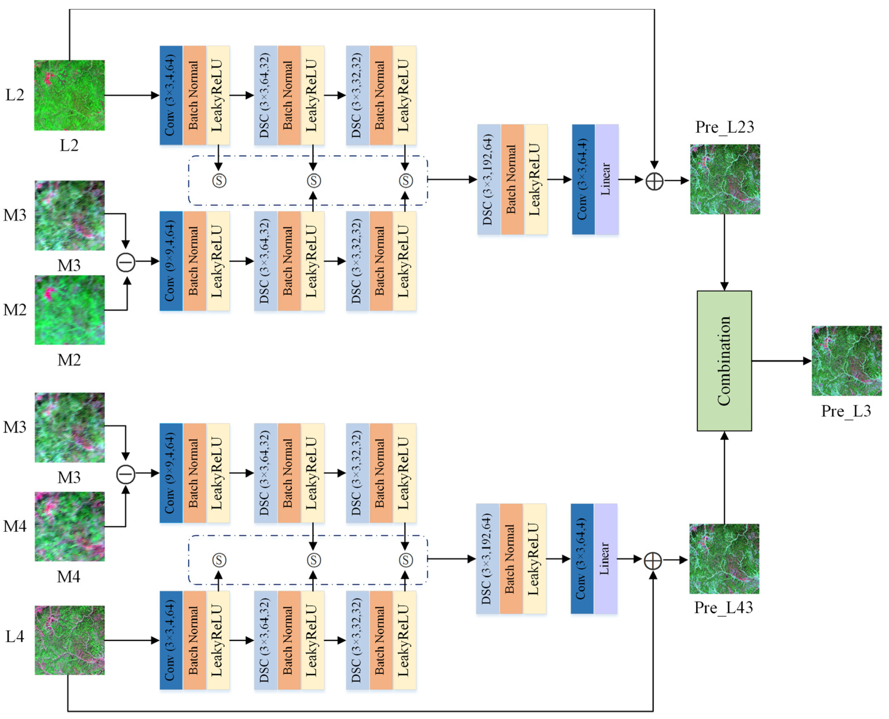
2.4.1. Architecture of STFDSC

Figure 2 illustrates the flowchart of STFDSC for reconstructing Landsat surface reflectance on T3 in Table 1. STFDSC is a two-stream model, with one stream predicting Landsat on T3 from Landsat on T2, as well as MODIS data on T2 and T3 (submodel 23) and the other stream predicting Landsat on T3 from Landsat on T4 and MODIS data on both T3 and T4 (submodel 43). The final predicted Landsat TM surface reflectance on T3 was obtained by combining both stream predictions.

For each submodel, the input data were Landsat at the base time and MODIS reflectance changes from the base time to the prediction time. The submodel consisted of three stages: (1) feature extraction of fine and coarse images; (2) feature fusion, and (3) prediction of surface reflectance at TM bands 2, 3, 4 and 7.

The feature extraction stage mainly extracted important features from Landsat data as well as from MODIS reflectance change over two dates using one standard convolution and two following DSCs. Coarse image features were extracted based on MODIS reflectance change instead of original MODIS reflectance in this study, which could provide direct temporal variations of reflectance in forest regions, and more importantly, reduce the number of model parameters and avoid network degradation [46].

DSC could significantly reduce the number of model parameters and had better performance when using similar amounts of model parameters with standard convolution [33]. To develop a lightweight CNN model, DSC was applied in both feature extraction and feature fusion. All convolution operations were followed by batch normalization in DSC, which could reduce internal covariate shift and allow us to use larger learning rates and thus speed up the optimization of hyperparameters [35]; moreover, previous studies suggested that saturated activation functions in CNN models, such as tanh and sigmoid, could suffer from exploding/vanishing gradient problems; we thus selected the non-saturated activation function LeakyReLU in the STFDSC [36].

In the feature fusion stage, the multilevel features generated in the feature extraction part were stacked. All produced features except the lowest-level features of MODIS reflectance change were incorporated in the STFDSC. The lowest-level features of MODIS reflectance change were not considered because coarse MODIS data contained less spatial information at this level. The DSC operation was performed on all stacked features. The prediction part included the prediction of fine-resolution residual images and their combination with Landsat data to finish one-stream surface reflectance reconstruction.

The final predicted result (Pre_L₃) was a weighted combination of two-stream predictions [47]. For each band, the weight was calculated according to the difference between each of the submodel predictions and the corresponding surface reflectance. A smaller difference corresponded to a higher weight.

$$Pre\_L_3=w_{23}\times Pre\_L_3^{2\to 3}+w_{43}\times Pre\_L_3^{4\to 3}$$

(1)

$$w_{23}=\frac{\left|\frac{1}{Pre\_L_3^{2\to 3}-M_3}\right|}{\left|\frac{1}{Pre\_L_3^{2\to 3}-M_3}\right|+\left|\frac{1}{Pre\_L_3^{4\to 3}-M_3}\right|}$$

(2)

$$w_{43}=\frac{\left|\frac{1}{Pre\_L_3^{4\to 3}-M_3}\right|}{\left|\frac{1}{Pre\_L_3^{2\to 3}-M_3}\right|+\left|\frac{1}{Pre\_L_3^{4\to 3}-M_3}\right|}$$

(3)

In this study, the STFDSC model was implemented in PyTorch deep learning framework.

2.4.2. Training

Two submodels in Figure 2 were trained separately. The parameters in feature extraction, feature fusion and prediction were jointly optimized using Adam. Submodel 24 was taken as an example. Input data for the training process included Landsat on T2, which was expressed as L₂, and MODIS residual image on T2 and T4 labeled by M₂₄ was computed as $M_{24}=M_4-M_2$, and the target image was Landsat on T4 (L₄). The loss function used in the optimization is expressed as:

$$loss={\displaystyle \sum _{i=1}^4\left(weigh{t}_i\times MAE\left(L_{4,i}-Pre\_L_{4,i}^{2\to 4}\right)\right)}+\frac{\lambda }{2}\times \parallel W{\parallel }^2$$

(4)

$$weigh{t}_i=\frac{{\left(mean{L}_{4,i}\right)}^{-1}}{{\displaystyle \sum _{j=1}^4{\left(mean{L}_{4,j}\right)}^{-1}}}$$

(5)

where $weigh{t}_i$ is the weight assigned for the i-th band, $MAE$ represents the mean absolute error, $L_{4,i}$ is the i-th band of L₄, $mean{L}_{4,j}$ is the average reflectance of the i-th band of L₄, and $Pre\_L_{4,i}^{2\to 4}$ is the predicted $L_{4,i}$ based on L₂, which is also the output of submodel 24 in the training process.

L2 regularization was included in the loss function to prevent overfitting. We assigned more weight to the band with smaller mean reflectance to reduce the problem that predictions at bands with smaller reflectance values were not accurate.

After the above steps, a trained submodel 24 was obtained. The trained model was then used to predict $Pre\_L_3^{2\to 3}$, as shown in Figure 2. Similarly, submodel 42 was trained and used to generate predictions $Pre\_L_3^{4\to 3}$.

2.5. Comparison of Experiments

To evaluate the impacts of the time intervals of the two nearest good-quality Landsat datasets on the prediction accuracy, we carried out the following three experiments in the ZWL and GKM (

Table 2. Comparison experiments carried out in the ZWL and GKM with different time intervals.

Study Area	Experiment	Time Intervals (Days) between the Left/Right Reference Image and Target Image
ZWL	T2/T3/T4	48/16
	T1/T3/T4	64/16
	T2/T3/T5	48/160
GKM	T2/T3/T4	16/16
	T1/T3/T4	48/16
	T2/T3/T5	16/32

). Comparisons of STFDSC with FSDAF, ESTARFM, EDCSTFN, and STFNET under these scenarios were also performed. Among these methods, the STFDSC, ESTARFM, EDCSTFN, and STFNET methods required two reference images as input. One reference image acquired before T3 and one reference image acquired after T3 were used to reconstruct Landsat imagery on T3 in all experiments. FSDAF required one reference image, and we used the Landsat reference data close to T3 in each experiment.

2.6. Generating Landsat Surface Reflectance Time Series

The STFDSC was then used to generate Landsat time series at 8-day intervals between two reference Landsat, which included Landsat from 15 June to 3 September for GKM, and from 25 February to 15 May for ZWL.

Due to cloud and residual atmospheric effects, gaps existed in the MODIS reflectance time series [48]. The linear interpolation method was used to generate spatially and temporally complete MODIS data time series before reconstructing Landsat data time series.

2.7. Accuracy Assessment

Evaluation indices included the root mean square error ($RMSE$), correlation coefficient ($CC$), and spectral angle mapper ($SAM$) index. The $SAM$ M index calculates the spectral angle between the reconstructed image and the observed Landsat reference image. Lower $SAM$, lower $RMSE$, and higher $CC$ values were associated with the higher quality of a reconstructed image. In this study, the average $RMSE$, $CC$, and $SAM$ values of the predicted reflectance compared with the observed reflectance on 2 August and 29 April were calculated for the GKM and ZWL, respectively.

$$RMS{E}_j=\sqrt{\frac{{\displaystyle {\sum }_{i=1}^n{(y_i-{\widehat{y}}_i)}^2}}{n}}$$

(6)

$$C{C}_j=\frac{{\displaystyle {\sum }_{i=1}^n(y_i-{\mu }_y)({\widehat{y}}_i-{\mu }_{\widehat{y}})}}{\sqrt{{\displaystyle {\sum }_{i=1}^n{(y_i-{\mu }_y)}^2}}\sqrt{{\displaystyle {\sum }_{i=1}^n{({\widehat{y}}_i-{\mu }_{\widehat{y}})}^2}}}$$

(7)

$$SAM=\frac{1}{n}{\displaystyle \sum _{i=1}^n\arccos \frac{{\displaystyle {\sum }_{j=1}^m\left(y_i^j{\widehat{y}}_i^j\right)}}{\sqrt{{\displaystyle {\sum }_{j=1}^m{\left(y_i^j\right)}^2}{\displaystyle {\sum }_{j=1}^m{\left({\widehat{y}}_i^j\right)}^2}}}}$$

(8)

where n is the number of pixels in an image, y is the observed reflectance, $\widehat{y}$ is the predicted reflectance, ${\mu }_y$ is the mean reflectance of the image, ${\mu }_{\widehat{y}}$ is the mean predicted reflectance of the image, j is the j-th band, and m is the number of bands.

In addition, pixels with NDVI values larger than 0.30 were extracted, and density scatter plots were then drawn based on 20,000 randomly selected pixels to further examine the differences between the observed reflectance and STF-predicted SR in forest pixels. Mean $MAE$ and bias were computed as follows.

$$MAE=\frac{1}{n}{\displaystyle \sum _{i=1}^n\left|\left(y_i-{\widehat{y}}_i\right)\right|}$$

(9)

$$bias=\frac{1}{n}{\displaystyle \sum _{i=1}^n\left({\widehat{y}}_i-y_i\right)}$$

(10)

3. Results

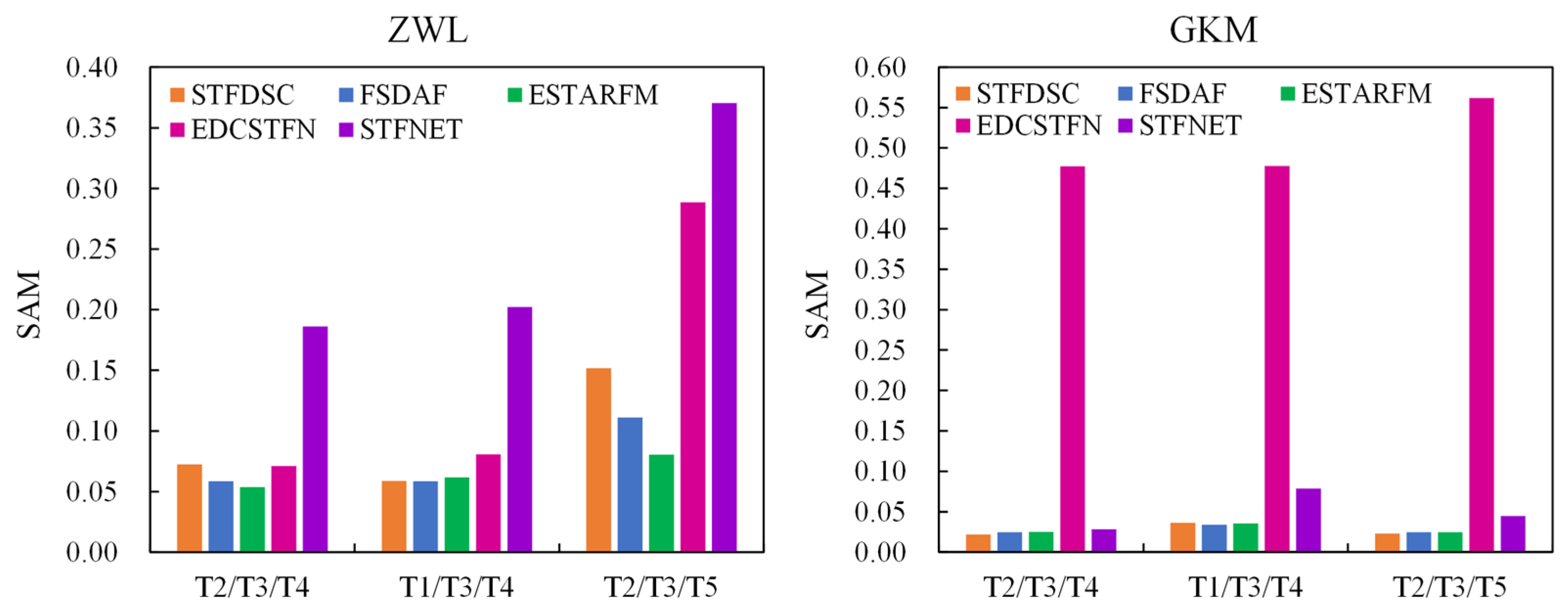
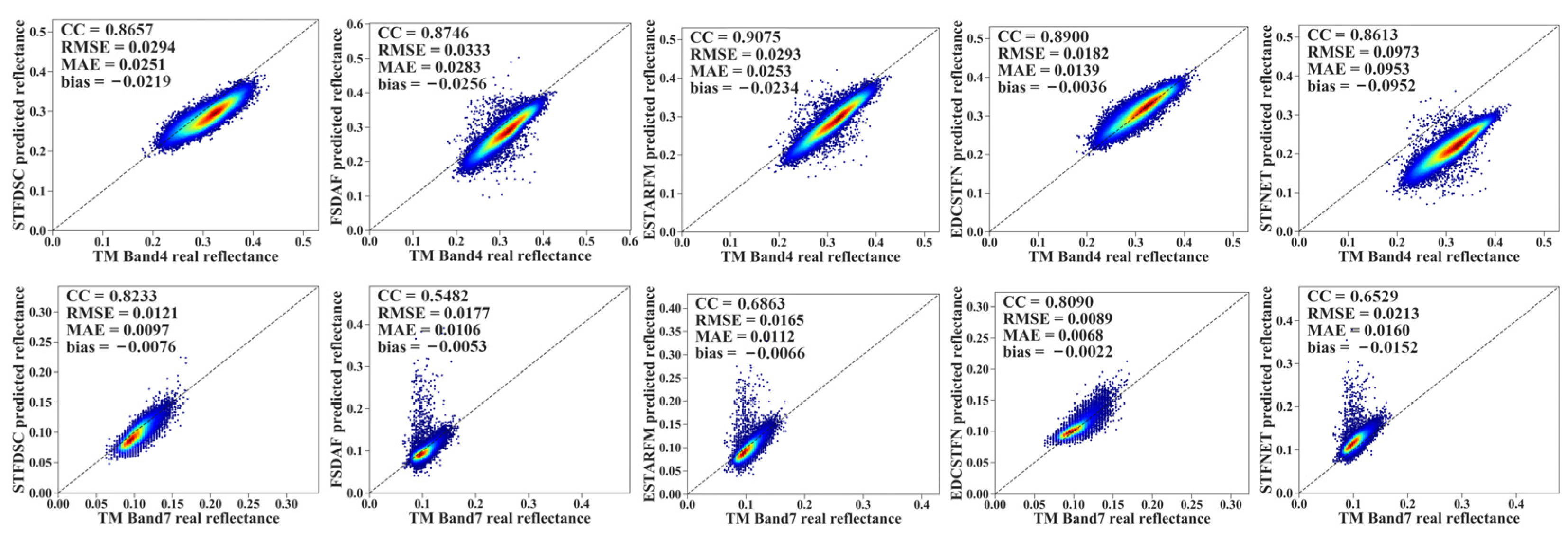
3.1. Performance of STF Methods in the Three Experiments

The evaluation indices calculated for the ZWL and GKM are shown in Figure 3 and Figure 4, respectively. In the ZWL, EDCSTFN generally had better performance in predicting Landsat surface reflectance, followed by STFDSC. The results of Experiment T2/T3/T4 indicated that STFDSC performed slightly better in predicting surface reflectance at TM band 3 than EDCSTFN, with an RMSE of 0.0176 and CC of 0.8747. In Experiment T1/T3/T4, STFDSC provided an overall more accurate fusion result in terms of RMSE, and ESTARFM provided comparable results. In Experiment T2/T3/T5, T2 and T5 had a time interval of 208 days, and T2 and T3 were at an interval of 48 days. Under this condition, two traditional methods, ESTARFM and FSDAF, had better prediction accuracy than the other three CNN-based fusion methods (Figure 3). FSDAF had the best performance because it required only one pair of data for prediction, and Landsat at T2 and MODIS at T2 and T3 served as inputs. When only a set of Landsat-MODIS data was available, FSDAF could be a suitable choice. STFDSC outperformed two other CNN methods and had CC values close to those of the traditional fusion methods. Using the SAM index, STFDSC even outperformed the two traditional methods and had the best performance.

Figure 3 shows that the RMSE of the STFNET prediction at TM band 4 was significantly larger than that of the other methods, which may have been caused by the large variation in reflectance. The mean reflectance was 0.1383 at T2 and 0.3172 at T4 in the ROI in the ZWL region. Significant variation in reflectance was not found in the GKM region, where STFNET had good performances (Figure 4).

Among the three experiments in the GKM, input data of Experiment T2/T3/T4 were Landsat data at T2 and T4 and MODIS data from T2-T4 acquired the closest to T3. The STFDSC results were much closer to the Landsat reference data than ESTARFM, FSDAF, EDCSTFN, and STFNET. For all four TM bands, the surface reflectance predicted by STFDSC had the lowest RMSE and highest CC values. In addition, STFDSC also corresponded to the lowest SAM index, 0.0219, suggesting the optimal accuracy achieved (Figure 4 and Figure 5). In Experiment T1/T3/T4, STFDSC still produced the most accurate synthetic image with an average RMSE of 0.0132 and CC of 0.8266. The surface reflectance generated by EDCSTFN was observed to be abnormal at TM band 3, partly due to its sensitivity to data preprocessing. We tried bilinear interpolation instead of the nearest neighbor method to preprocess the MODIS data and found that it performed normally in the GKM. The main reason for the observed abnormal phenomena was probably that the mean reflectance at TM band 3 was 0.0304, substantially lower than 0.3036 at TM band 4 and 0.0615 at band 7, and fluctuations existed in predicting lower reflectance by EDCSTFN. In this study, the loss function adopted the weighted average method, in which bands with smaller mean reflectance were assigned a larger weight to avoid substantial prediction error at TM band 3; therefore, compared with EDCSTFN and STFNET, STFDSC produced a more stable and accurate results, which also suggested its better performance in generating Landsat surface reflectance. In Experiment T2/T3/T5, STFDSC still achieved the best prediction accuracy, with an average RMSE of 0.0081, CC of 0.9314, and SAM of 0.0228 (Figure 4 and Figure 5).

3.2. Performance of STF Methods in Deriving the NDVI and NBR

We calculated the NDVI and NBR from fused Landsat surface reflectance. As shown in

Table 3. Performances of five STF methods in reconstructing the NDVI and NBR.

Method	ZWL				GKM
	NDVI RMSE	NDVI CC	NBR RMSE	NBR CC	NDVI RMSE	NDVI CC	NBR RMSE	NBR CC
STFDSC	0.0677	0.8825	0.0526	0.9268	0.0226	0.9114	0.0281	0.8891
FSDAF	0.0726	0.8455	0.0543	0.9361	0.0288	0.8509	0.0339	0.8433
ESTARFM	0.0696	0.8669	0.0482	0.9444	0.0262	0.8685	0.0354	0.8338
EDCSTFN	0.0800	0.9005	0.0457	0.9467	4.6585	−0.0406	0.0353	0.8202
STFNET	0.1386	0.8656	0.2198	0.9287	0.0345	0.8682	0.0342	0.8649

, STFDSC provided the most accurate NDVI in the ZWL and GKM, with RMSEs of 0.0677 and 0.0226, respectively. In addition, STFDSC obtained the closest result to the reference NBR derived from Landsat data in the GKM, with an RMSE of 0.0281 and CC of 0.8891. In the ZWL, EDCSTFN produced slightly better NBR results than STFDSC, with RMSEs of 0.0457 and 0.9467. These results suggested that surface reflectance generated by STFDSC could be used to derive vegetation indices accurately.

Moreover, we extracted the pixels with NDVI values larger than 0.30 and then randomly selected 20,000 pixels and drew the density plot of selected pixel TM band 4 and band 7 under the T2/T3/T4 experiment. The results are shown in Figure 6. All fusion methods, except EDCSTFN, underestimated the near-infrared reflectance in the ZWL. The underestimation of STFNET prediction was particularly serious, with a negative bias of 0.0935. The problem could be explained by the algorithm principle. Both STFDSC and STFNET contained two submodels that combined MODIS reflectance change and Landsat data to compute the weight, and predictions were the weighted average of results from the two submodels. ESTARFM and FSDAF also predicted the target Landsat data based on the differences in MODIS reflectance. In the ZWL, the mean MODIS reflectance change was 0.1485 from T2 to T3 and 0.0413 from T3 to T4, corresponding to Landsat reflectance changes of 0.1627 and 0.0162, respectively. MODIS reflectance change was less than Landsat reflectance change from T2 to T3, while from T3 to T4, MODIS reflectance change was larger than Landsat reflectance change, which made the predictions to be far from the reference. EDCSTFN used the MODIS and Landsat reflectance data without incorporating their changes over time and thus avoided the underestimation caused by the observed violation. In TM band 7, EDCSTFN achieved the best accuracy in terms of CC, RMSE, and MAE, followed by STFDSC. The results in the GKM are shown in Figure 7. STFDSC had the best prediction accuracy, followed by STFNET. EDCSTFN generally overestimated Landsat reflectance at both band 4 and band 7.

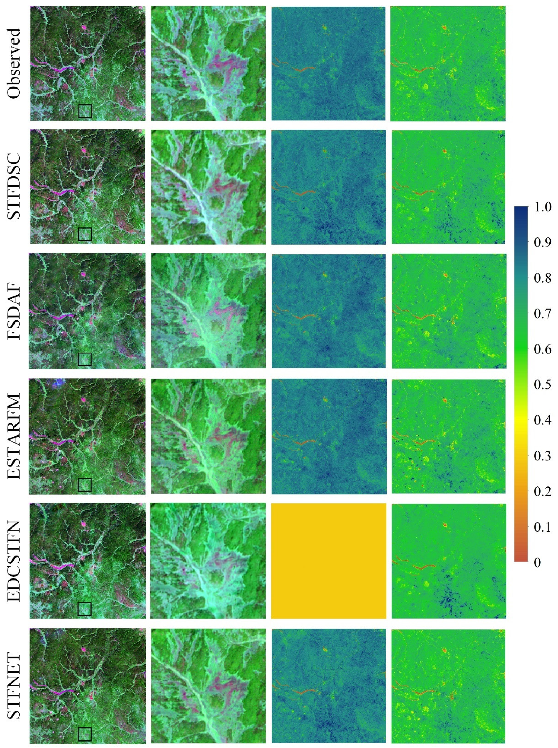
3.3. Visual Assessment of the Five STF Fusion Methods

Figure 8 shows the prediction results of the five fusion algorithms in the ZWL under Experiment T2/T3/T4. Due to cloud contamination of Landsat data on T4, the fusion results of FSDAF, ESTARFM and STFNET were severely affected, where clouds and cloud shadows were clearly observed. In contrast, no obvious cloud or shadow existed in the STFDSC and EDCSTFN reconstructed images, suggesting the robustness of the STFDSC and EDCSTFN fusion methods; however, EDCSTFN likely failed to capture spatial details, and the corresponding prediction results were more obscured than those from other STF methods. NDVI and NBR data calculated from fused reflectance by STFDSC were also close to the real data in the first row (Figure 8). These results demonstrated the optimal performance of STFDSC in generating Landsat surface reflectance.

Figure 9 shows the performance of the five STF methods in the GKM based on Experiment T2/T3/T4. The predicted results of STFDSC were shown to be very similar to those of the Landsat reference image in color, especially in the middle and lower right of the image in the first column. The spatial distribution of the NDVI and NBR in Figure 9 also suggested the better performance of the STFDSC method; however, in forests with a higher density such as in the lower right corner, significant differences between observations and STFDSC predictions were found. Due to the large errors in surface reflectance prediction at TM band 3, abnormal EDCSTFN NDVI values were observed.

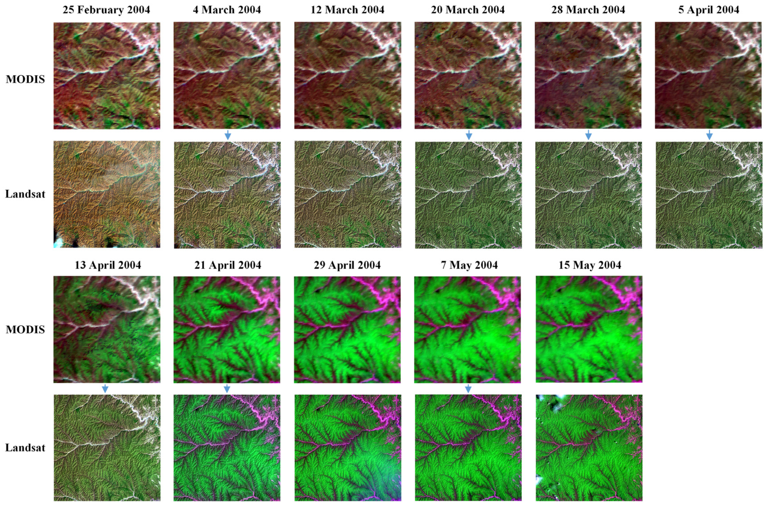
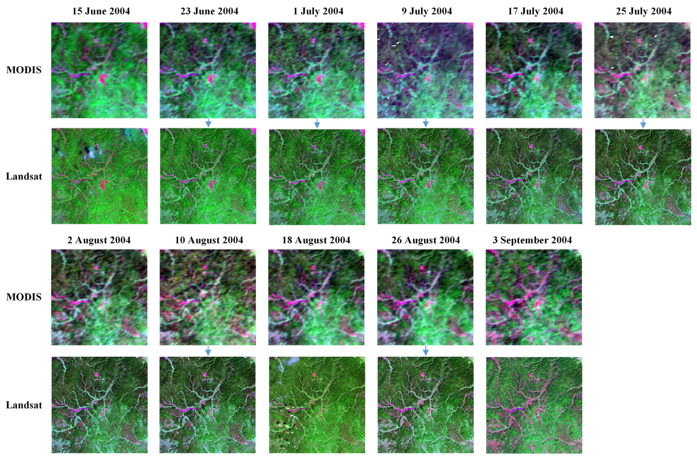
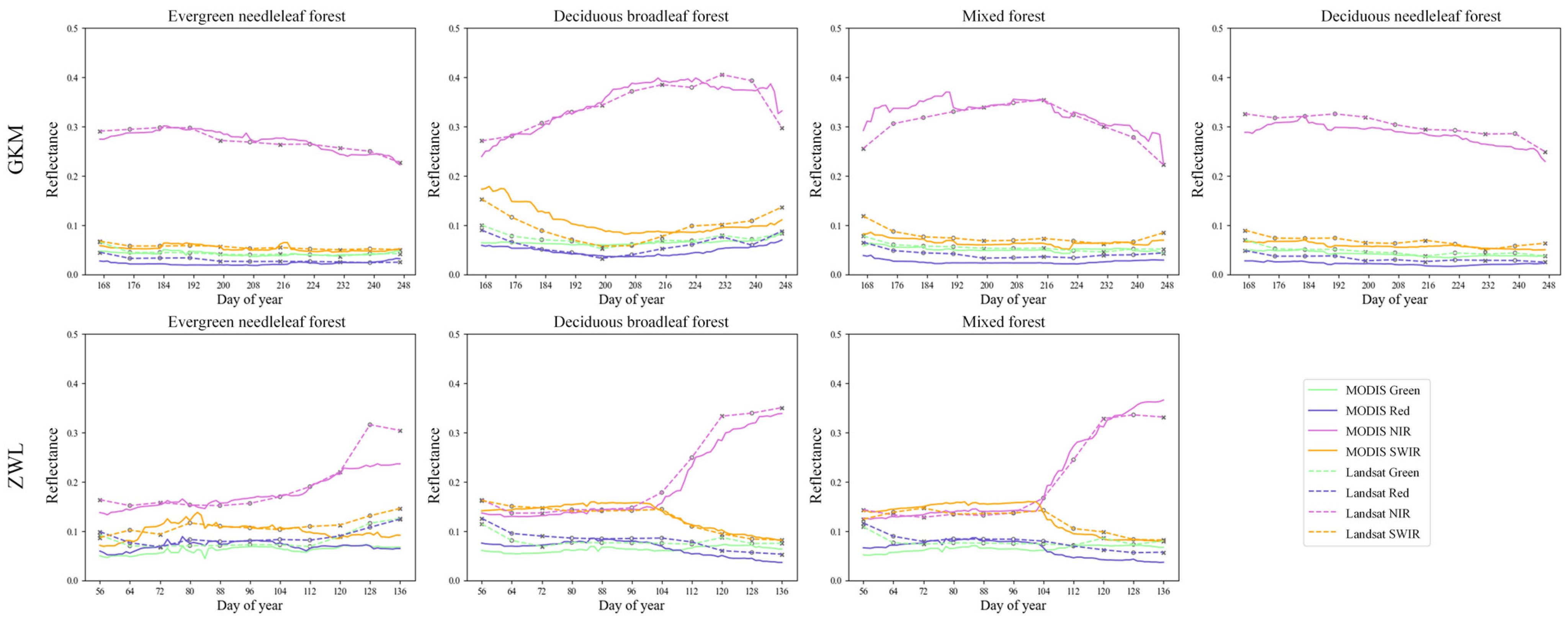
3.4. Landsat Surface Reflectance Time Series Generated Using STFDSC

Landsat data time series from 25 February to 15 May 2004 at 8-day intervals in the ZWL region were shown in Figure 10. We did not predict the Landsat data from 15 May to 6 October, because the two reference data had an interval of 144-day in acquisition time, and STFDSC was not quite suitable for prediction with longer time series without any observation, as shown in Figure 3.

According to the MODIS data time series, significant greening occurred between 5 April and 21 April, which was well captured by reconstructed Landsat data. For Landsat data at reference time periods, such as 25 February, 29 April, and 15 May 2004, some pixels were contaminated by cloud; however, the phenomenon was not observed from Landsat data at prediction times, which indicated that the introduction of MODIS data could improve Landsat predictions to some degree. These results were also established for Landsat data time series from 15 June to 3 September 2004 in the GKM region, suggesting the rationality of STFDSC to generate Landsat data time series (Figure 11). The gaps in MODIS data (e.g., on 9 July and 25 July) did not greatly affect the accuracy of reconstructed Landsat due to the preprocess of MODIS data gaps before prediction. We extracted MODIS and Landsat reference at the green, red, near-infrared, and shortwave infrared bands of different forest types in GKM and ZWL, and results showed that Landsat reflectance data were similar to or even better than MODIS data in temporal trajectories (Figure 12).

4. Discussion

We proposed the STFDSC method to predict Landsat data time series, which contains low-level and middle-level features that have been widely ignored in most STF-related CNN models [29,49]. The usage of multilevel feature information could be the major reason for its better performance demonstrated in this study.

To build an efficient CNN, we used the DSC in the architecture of STFDSC, which was especially suitable for mobile and embedded vision applications [50]. The combined use of DSC and some efficiency tricks (e.g., residual structure, BatchNorm) can prevent the overfitting and speed up network convergence. Compared with EDCSTFN, the number of trainable parameters in STFDSC was less. For the prediction of the target image with a size of 4 × 150 × 150, the forward propagation floating-point computation required by the two methods as shown in

Table 4. The number of trainable parameters and forward propagated floating-point operations of the three CNN-based STF methods.

Method	Trainable Parameters	Million FLOPs
STFNET	70,376	1583.5
STFDSC	97,288	2220.7
EDCSTFN	281,764	10,600.7

. STFNET was the lightest model, but at the cost of sacrificing prediction accuracy.

Since surface reflectance at four TM bands varied in a wide range (e.g., from 0.0305 at TM band 3 to 0.3036 at TM band 4 in the GKM), the band with higher reflectance tended to contribute more to the loss function when the weight factor was not included. Therefore, we adopted the weighted loss function in STFDSC, assigning the weight for each band according to the mean surface reflectance value; this could ensure the stability of STFDSC in predicting surface reflectance at the band with small reflectance values to some degree. We also obtained the final predicted reflectance using the weighted average of the two-stream prediction results, which also reduced the variation in the forecast results.

It should be noted that, similar to other STF methods, high-quality reference data were required in STFDSC; however, this requirement could not be met in practical applications, or the two nearest reference data points on the acquisition date may have a long-time interval, which could possibly cause a large bias in the predictions. In some cases, only Landsat images with heavy cloud cover are available, particularly in tropical forests; it would be necessary to consider how to fuse with auxiliary data sources such as SAR data [51].

The proposed STFDSC could be a unified framework for fusing datasets from different sensors, including but not limited to Landsat and MODIS data. Future research could be conducted on the generation of higher spatial or temporal satellite images, such as through the fusion of WorldView-2 or Sentinel-2 images using the STFDSC algorithm [52,53], and higher-level processed satellite data products, such as the leaf area index and land surface temperature [47,54,55].

5. Conclusions

We proposed an STFDSC method for reconstructing Landsat surface reflectance from Landsat and MODIS data. The performance was evaluated in the GKM and ZWL forest regions of China, and comparisons with four published fusion methods, FSDAF, ESTARFM, EDCSTFN and STFNET, were also carried out. The results suggest that the STFDSC based results were much closer to Landsat reference data in the GKM than ESTARFM, FSDAF, EDCSTFN, and STFNET. EDCSTFN performed slightly better than STFDSC in ZWL, but produced abnormal predictions at TM band 3 in the GKM; moreover, the NDVI and NBR calculated from Landsat surface reflectance generated by STFDSC were very close to those obtained from Landsat reference data. The results indicated that the STFDSC proposed in this study had stable and accurate predictions in both the GKM and ZWL. Based on STFDSC, Landsat reflectance time series at 8-day temporal resolution were also reconstructed in two regions. Although STFDSC was designed to generate reflectance time series in this study, it could be used to integrate higher-level processed satellite data products such as the leaf area index and land surface temperature, which needs to be investigated in future studies.

References

1. Woodcock, C.E.; Allen, R.; Anderson, M.; Belward, A.; Bindschadler, R.; Cohen, W.; Gao, F.; Goward, S.N.; Helder, D.; Helmer, E.; et al. Free Access to Landsat Imagery. Science 2008, 320, 11011. [Google Scholar] [CrossRef] [PubMed]
2. Wulder, M.A.; Loveland, T.R.; Roy, D.P.; Crawford, C.J.; Masek, J.G.; Woodcock, C.E.; Allen, R.G.; Anderson, M.C.; Belward, A.S.; Cohen, W.B.; et al. Current status of Landsat program, science, and applications. Remote Sens. Environ. 2019, 225, 127–147. [Google Scholar] [CrossRef]
3. Nguyen, T.H.; Jones, S.; Soto-Berelov, M.; Haywood, A.; Hislop, S. Landsat Time-Series for Estimating Forest Aboveground Biomass and Its Dynamics across Space and Time: A Review. Remote Sens. 2020, 12, 98. [Google Scholar] [CrossRef] [Green Version]
4. Bolton, D.K.; Gray, J.M.; Melaas, E.K.; Moon, M.; Eklundh, L.; Friedl, M.A. Continental-scale land surface phenology from harmonized Landsat 8 and Sentinel-2 imagery. Remote Sens. Environ. 2020, 240, 111685. [Google Scholar] [CrossRef]
5. Huang, H.; Chen, Y.; Clinton, N.; Wang, J.; Wang, X.; Liu, C.; Gong, P.; Yang, J.; Bai, Y.; Zheng, Y.; et al. Mapping major land cover dynamics in Beijing using all Landsat images in Google Earth Engine. Remote Sens. Environ. 2017, 202, 166–176. [Google Scholar] [CrossRef]
6. Zhu, Z.; Woodcock, C.E. Continuous change detection and classification of land cover using all available Landsat data. Remote Sens. Environ. 2014, 144, 152–171. [Google Scholar] [CrossRef] [Green Version]
7. Chen, B.; Xiao, X.; Li, X.; Pan, L.; Doughty, R.; Ma, J.; Dong, J.; Qin, Y.; Zhao, B.; Wu, Z.; et al. A mangrove forest map of China in 2015: Analysis of time series Landsat 7/8 and Sentinel-1A imagery in Google Earth Engine cloud computing platform. ISPRS J. Photogramm. Remote Sens. 2017, 131, 104–120. [Google Scholar] [CrossRef]
8. Powell, S.L.; Cohen, W.B.; Healey, S.P.; Kennedy, R.E.; Moisen, G.G.; Pierce, K.B.; Ohmann, J.L. Quantification of live aboveground forest biomass dynamics with Landsat time-series and field inventory data: A comparison of empirical modeling approaches. Remote Sens. Environ. 2010, 114, 1053–1068. [Google Scholar] [CrossRef]
9. White, J.C.; Wulder, M.A.; Hermosilla, T.; Coops, N.C.; Hobart, G.W. A nationwide annual characterization of 25 years of forest disturbance and recovery for Canada using Landsat time series. Remote Sens. Environ. 2017, 194, 303–321. [Google Scholar] [CrossRef]
10. Griffiths, P.; Kuemmerle, T.; Baumann, M.; Radeloff, V.C.; Abrudan, I.V.; Lieskovsky, J.; Munteanu, C.; Ostapowicz, K.; Hostert, P. Forest disturbances, forest recovery, and changes in forest types across the Carpathian ecoregion from 1985 to 2010 based on Landsat image composites. Remote Sens. Environ. 2014, 151, 72–88. [Google Scholar] [CrossRef]
11. Yan, L.; Roy, D.P. Large-Area Gap Filling of Landsat Reflectance Time Series by Spectral-Angle-Mapper Based Spatio-Temporal Similarity (SAMSTS). Remote Sens. 2018, 10, 609. [Google Scholar] [CrossRef] [Green Version]
12. Meng, Q.; Cooke, W.H.; Rodgers, J. Derivation of 16-day time-series NDVI data for environmental studies using a data assimilation approach. GIScience Remote Sens. 2013, 50, 500–514. [Google Scholar] [CrossRef]
13. Gao, F.; Masek, J.; Schwaller, M.; Hall, F. On the blending of the Landsat and MODIS surface reflectance: Predicting daily Landsat surface reflectance. IEEE Trans. Geosci. Remote Sens. 2006, 44, 2207–2218. [Google Scholar] [CrossRef]
14. Zhou, J.; Chen, J.; Chen, X.; Zhu, X.; Qiu, Y.; Song, H.; Rao, Y.; Zhang, C.; Cao, X.; Cui, X. Sensitivity of six typical spatiotemporal fusion methods to different influential factors: A comparative study for a normalized difference vegetation index time series reconstruction. Remote Sens. Environ. 2021, 252, 112130. [Google Scholar] [CrossRef]
15. Weng, Q.; Fu, P.; Gao, F. Generating daily land surface temperature at Landsat resolution by fusing Landsat and MODIS data. Remote Sens. Environ. 2014, 145, 55–67. [Google Scholar] [CrossRef]
16. Cammalleri, C.; Anderson, M.C.; Gao, F.; Hain, C.R.; Kustas, W.P. Mapping daily evapotranspiration at field scales over rainfed and irrigated agricultural areas using remote sensing data fusion. Agric. For. Meteorol. 2014, 186, 1–11. [Google Scholar] [CrossRef] [Green Version]
17. Hilker, T.; Wulder, M.A.; Coops, N.C.; Seitz, N.; White, J.C.; Gao, F.; Masek, J.G.; Stenhouse, G. Generation of dense time series synthetic Landsat data through data blending with MODIS using a spatial and temporal adaptive reflectance fusion model. Remote Sens. Environ. 2009, 113, 1988–1999. [Google Scholar] [CrossRef]
18. Zhu, X.; Chen, J.; Gao, F.; Chen, X.; Masek, J.G. An enhanced spatial and temporal adaptive reflectance fusion model for complex heterogeneous regions. Remote Sens. Environ. 2010, 114, 2610–2623. [Google Scholar] [CrossRef]
19. Dao, P.D.; Mong, N.T.; Chan, H.-P. Landsat-MODIS image fusion and object-based image analysis for observing flood inundation in a heterogeneous vegetated scene. GISci. Remote Sens. 2019, 56, 1148–1169. [Google Scholar] [CrossRef]
20. Wu, M.; Niu, Z.; Wang, C.; Wu, C.; Wang, L. Use of MODIS and Landsat time series data to generate high-resolution temporal synthetic Landsat data using a spatial and temporal reflectance fusion model. J. Appl. Remote Sens. 2012, 6, 063507. [Google Scholar]
21. Huang, B.; Zhang, H. Spatio-temporal reflectance fusion via unmixing: Accounting for both phenological and land-cover changes. Int. J. Remote Sens. 2014, 35, 6213–6233. [Google Scholar] [CrossRef]
22. Gevaert, C.M.; García-Haro, F.J. A comparison of STARFM and an unmixing-based algorithm for Landsat and MODIS data fusion. Remote Sens. Environ. 2015, 156, 34–44. [Google Scholar] [CrossRef]
23. Zhu, X.; Helmer, E.H.; Gao, F.; Liu, D.; Chen, J.; Lefsky, M.A. A flexible spatiotemporal method for fusing satellite images with different resolutions. Remote Sens. Environ. 2016, 172, 165–177. [Google Scholar] [CrossRef]
24. Hong, D.; Yokoya, N.; Chanussot, J.; Zhu, X.X. An Augmented Linear Mixing Model to Address Spectral Variability for Hyperspectral Unmixing. IEEE Trans. Image Processing 2019, 28, 1923–1938. [Google Scholar] [CrossRef] [Green Version]
25. Tan, Z.; Di, L.; Zhang, M.; Guo, L.; Gao, M. An Enhanced Deep Convolutional Model for Spatiotemporal Image Fusion. Remote Sens. 2019, 11, 2898. [Google Scholar] [CrossRef] [Green Version]
26. Huang, B.; Song, H. Spatiotemporal Reflectance Fusion via Sparse Representation. IEEE Trans. Geosci. Remote Sens. 2012, 50, 3707–3716. [Google Scholar] [CrossRef]
27. Song, H.; Huang, B. Spatiotemporal Satellite Image Fusion Through One-Pair Image Learning. IEEE Trans. Geosci. Remote Sens. 2013, 51, 1883–1896. [Google Scholar] [CrossRef]
28. Song, H.; Liu, Q.; Wang, G.; Hang, R.; Huang, B. Spatiotemporal Satellite Image Fusion Using Deep Convolutional Neural Networks. IEEE J. Sel. Top. Appl. Earth Obs. Remote Sens. 2018, 11, 821–829. [Google Scholar] [CrossRef]
29. Liu, X.; Deng, C.; Chanussot, J.; Hong, D.; Zhao, B. StfNet: A Two-Stream Convolutional Neural Network for Spatiotemporal Image Fusion. IEEE Trans. Geosci. Remote Sens. 2019, 57, 6552–6564. [Google Scholar] [CrossRef]
30. Li, W.; Zhang, X.; Peng, Y.; Dong, M. Spatiotemporal Fusion of Remote Sensing Images using a Convolutional Neural Network with Attention and Multiscale Mechanisms. Int. J. Remote Sens. 2021, 42, 1973–1993. [Google Scholar] [CrossRef]
31. Chen, B.; Li, J.; Jin, Y.F. Deep Learning for Feature-Level Data Fusion: Higher Resolution Reconstruction of Historical Landsat Archive. Remote Sens. 2021, 13, 167. [Google Scholar] [CrossRef]
32. Gao, J.; Yuan, Q.; Li, J.; Zhang, H.; Su, X. Cloud Removal with Fusion of High Resolution Optical and SAR Images Using Generative Adversarial Networks. Remote Sens. 2020, 12, 191. [Google Scholar] [CrossRef] [Green Version]
33. Chollet, F. Xception: Deep Learning with Depthwise Separable Convolutions. In Proceedings of the 2017 IEEE Conference on Computer Vision and Pattern Recognition (CVPR), Honolulu, HI, USA, 21–26 July 2017; pp. 1800–1807. [Google Scholar]
34. Lin, T.Y.; Dollar, P.; Girshick, R.; He, K.; Hariharan, B.; Belongie, S. Feature Pyramid Networks for Object Detection. In Proceedings of the 2017 IEEE Conference on Computer Vision and Pattern Recognition (CVPR), Honolulu, HI, USA, 21–26 July 2017. [Google Scholar]
35. Ioffe, S.; Szegedy, C. Batch normalization: Accelerating deep network training by reducing internal covariate shift. In Proceedings of the 32nd International Conference on International Conference on Machine Learning, Lille, France, 6–11 July 2015; Volume 37, pp. 448–456. [Google Scholar]
36. Xu, B.; Wang, N.; Chen, T.; Li, M. Empirical Evaluation of Rectified Activations in Convolutional Network. arXiv 2015, arXiv:1505.00853. [Google Scholar]
37. Fu, Y.; He, H.S.; Zhao, J.; Larsen, D.R.; Zhang, H.; Sunde, M.G.; Duan, S. Climate and Spring Phenology Effects on Autumn Phenology in the Greater Khingan Mountains, Northeastern China. Remote Sens. 2018, 10, 449. [Google Scholar] [CrossRef] [Green Version]
38. Guo, X.-y.; Zhang, H.-y.; Wang, Y.-q.; Zhao, J.-j.; Zhang, Z.-x. The driving factors and their interactions of fire occurrence in Greater Khingan Mountains, China. J. Mt. Sci. 2020, 17, 2674–2690. [Google Scholar] [CrossRef]
39. Kang, D.; Guo, Y.; Ren, C.; Zhao, F.; Feng, Y.; Han, X.; Yang, G. Population Structure and Spatial Pattern of Main Tree Species in Secondary Betula platyphylla Forest in Ziwuling Mountains, China. Sci. Rep. 2014, 4, 6873. [Google Scholar] [CrossRef] [Green Version]
40. Zheng, F.; He, X.; Gao, X.; Zhang, C.-e.; Tang, K. Effects of erosion patterns on nutrient loss following deforestation on the Loess Plateau of China. Agric. Ecosyst. Environ. 2005, 108, 85–97. [Google Scholar] [CrossRef]
41. Li, C.; Wang, J.; Hu, L.; Yu, L.; Clinton, N.; Huang, H.; Yang, J.; Gong, P. A Circa 2010 Thirty Meter Resolution Forest Map for China. Remote Sens. 2014, 6, 5325–5343. [Google Scholar] [CrossRef] [Green Version]
42. USGS. Landsat Collection 1 Level 1 Product Definition; United State Geological Survey: Reston, VA, USA, 2019.
43. Hislop, S.; Jones, S.; Soto-Berelov, M.; Skidmore, A.; Haywood, A.; Nguyen, T.H. Using Landsat Spectral Indices in Time-Series to Assess Wildfire Disturbance and Recovery. Remote Sens. 2018, 10, 460. [Google Scholar] [CrossRef] [Green Version]
44. Walker, J.J.; de Beurs, K.M.; Wynne, R.H.; Gao, F. Evaluation of Landsat and MODIS data fusion products for analysis of dryland forest phenology. Remote Sens. Environ. 2012, 117, 381–393. [Google Scholar] [CrossRef]
45. Walker, J.J.; de Beurs, K.M.; Wynne, R.H. Dryland vegetation phenology across an elevation gradient in Arizona, USA, investigated with fused MODIS and Landsat data. Remote Sens. Environ. 2014, 144, 85–97. [Google Scholar] [CrossRef]
46. He, K.; Zhang, X.; Ren, S.; Sun, J. Deep Residual Learning for Image Recognition. In Proceedings of the 2016 IEEE Conference on Computer Vision and Pattern Recognition (CVPR), Las Vegas, NV, USA, 27–30 June 2016; pp. 770–778. [Google Scholar]
47. Yin, Z.X.; Wu, P.H.; Foody, G.M.; Wu, Y.L.; Liu, Z.H.; Du, Y.; Ling, F. Spatiotemporal Fusion of Land Surface Temperature Based on a Convolutional Neural Network. IEEE Trans. Geosci. Remote Sens. 2021, 59, 1808–1822. [Google Scholar] [CrossRef]
48. Ju, J.; Roy, D.P.; Shuai, Y.; Schaaf, C. Development of an approach for generation of temporally complete daily nadir MODIS reflectance time series. Remote Sens. Environ. 2010, 114, 1–20. [Google Scholar] [CrossRef]
49. Li, Y.; Li, J.; He, L.; Chen, J.; Plaza, A. A new sensor bias-driven spatio-temporal fusion model based on convolutional neural networks. Sci. China Inf. Sci. 2020, 63, 140302. [Google Scholar] [CrossRef] [Green Version]
50. Howard, A.G.; Zhu, M.; Chen, B.; Kalenichenko, D.; Wang, W.; Weyand, T.; Andreetto, M.; Adam, H. MobileNets: Efficient Convolutional Neural Networks for Mobile Vision Applications. arXiv 2017, arXiv:1704.04861. [Google Scholar]
51. Hirschmugl, M.; Deutscher, J.; Sobe, C.; Bouvet, A.; Mermoz, S.; Schardt, M. Use of SAR and Optical Time Series for Tropical Forest Disturbance Mapping. Remote Sens. 2020, 12, 727. [Google Scholar] [CrossRef] [Green Version]
52. Nikolakopoulos, K.; Oikonomidis, D. Quality assessment of ten fusion techniques applied on Worldview-2. Eur. J. Remote Sens. 2015, 48, 141–167. [Google Scholar] [CrossRef]
53. Ao, Z.; Sun, Y.; Xin, Q. Constructing 10-m NDVI Time Series From Landsat 8 and Sentinel 2 Images Using Convolutional Neural Networks. IEEE Geosci. Remote Sens. Lett. 2021, 18, 1461–1465. [Google Scholar] [CrossRef]
54. Sadeh, Y.; Zhu, X.; Dunkerley, D.; Walker, J.P.; Zhang, Y.; Rozenstein, O.; Manivasagam, V.S.; Chenu, K. Fusion of Sentinel-2 and PlanetScope time-series data into daily 3 m surface reflectance and wheat LAI monitoring. Int. J. Appl. Earth Obs. Geoinf. 2021, 96, 102260. [Google Scholar] [CrossRef]
55. Hernández, C.; Nunes, L.; Lopes, D.; Graña, M. Data fusion for high spatial resolution LAI estimation. Inf. Fusion 2014, 16, 59–67. [Google Scholar] [CrossRef]
Figure 1. Location of the study area, region of interest (purple regions in Box 1 and Box 2), and coverages of Landsat 5 scenes labeled by Worldwide Reference System 2 (WRS-2) path/row for the study area in the Greater Khingan Mountains (GKM, Box 1) and Ziwuling Mountains (ZWL, Box 2). The background data showed different forest types from Li et al. [41] with mapped colors described in the legend.
Remotesensing 14 02199 g001
Figure 2. Architecture of the STFDSC model. Inputs of the STFDSC model were Landsat and MODIS data at base times (L2, L4, M2, and M4), and MODIS data at the prediction time (M3). Pre_L23 and Pre_L43 were predicted Landsat data using two sub-models, and Pre_L3 was the final Landsat prediction and obtained by weighted average of Pre_L23 and Pre_L43.
Remotesensing 14 02199 g002
Figure 3. Performance of five STF methods in reconstructing Landsat surface reflectance in the ZWL.
Remotesensing 14 02199 g003
Figure 4. Performance of five STF methods in reconstructing Landsat surface reflectance in the GKM.
Remotesensing 14 02199 g004
Figure 5. Performance of five STF methods in terms of the SAM index in the ZWL and GKM.
Remotesensing 14 02199 g005
Figure 6. Density scatter plot of the observed reflectance and predicted reflectance at TM bands 4 and 7 in the ZWL.
Remotesensing 14 02199 g006
Figure 7. Scatter density plot of the observed reflectance and predicted reflectance at TM band 4 and band 7 in the GKM.
Remotesensing 14 02199 g007
Figure 8. Fusion results on 29 April in the ZWL region. The first column shows the TM band 7-4-2 composite images of the reference image and five STF methods; the second column shows the zoomed-in details of the black rectangle in the first column; the third column shows the calculated NDVI, and the last column shows the calculated NBR.
Remotesensing 14 02199 g008
Figure 9. Fusion results on 2 August in the GKM region. The first column shows the TM band 7-4-2 composite images of the reference image and five STF methods; the second column shows the zoomed-in details of the black rectangle in the first column; the third column shows the calculated NDVI, and the last column shows the calculated NBR.
Remotesensing 14 02199 g009
Figure 10. MODIS and Landsat data time series from 25 February to 15 May 2004 in the ZWL region. TM images were shown using the 7-4-2 band combination, and MODIS images were shown using the 7-2-4 band combination. The blue arrow between MODIS and Landsat represented that the corresponding Landsat data were reconstructed, rather than the observed reference image.
Remotesensing 14 02199 g010
Figure 11. MODIS and Landsat data time series from 15 June to 3 September 2004 in the GKM region. TM images were shown using the 7-4-2 band combination, and MODIS images were shown using the 7-2-4 band combination. The blue arrow between MODIS and Landsat represented that the corresponding Landsat data were reconstructed, rather than the observed reference image.
Remotesensing 14 02199 g011
Figure 12. MODIS and Landsat reflectance time series of different forest types in GKM and ZWL regions. The top row represented the temporal trajectories of reflectance in GKM, and the bottom row corresponded to temporal trajectories of reflectance in ZWL.
Remotesensing 14 02199 g012