
Urban Sprawl and COVID-19 Impact Analysis by Integrating Deep Learning with Google Earth Engine


Abstract
:1. Introduction
2. Tools
2.1. Google Earth Engine
2.2. TensorFlow
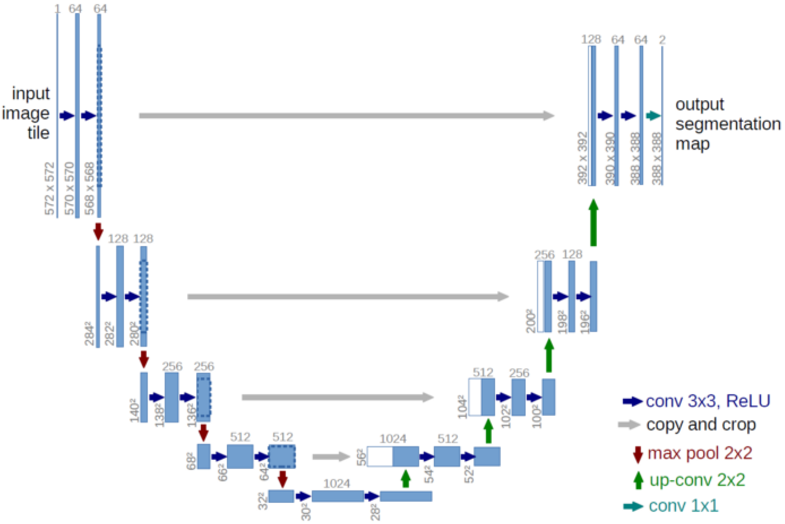
2.3. Neural Network
3. Framework for Urban Sprawl Analysis
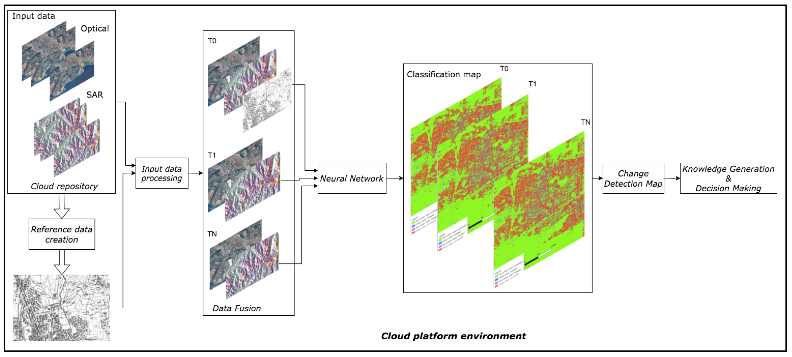
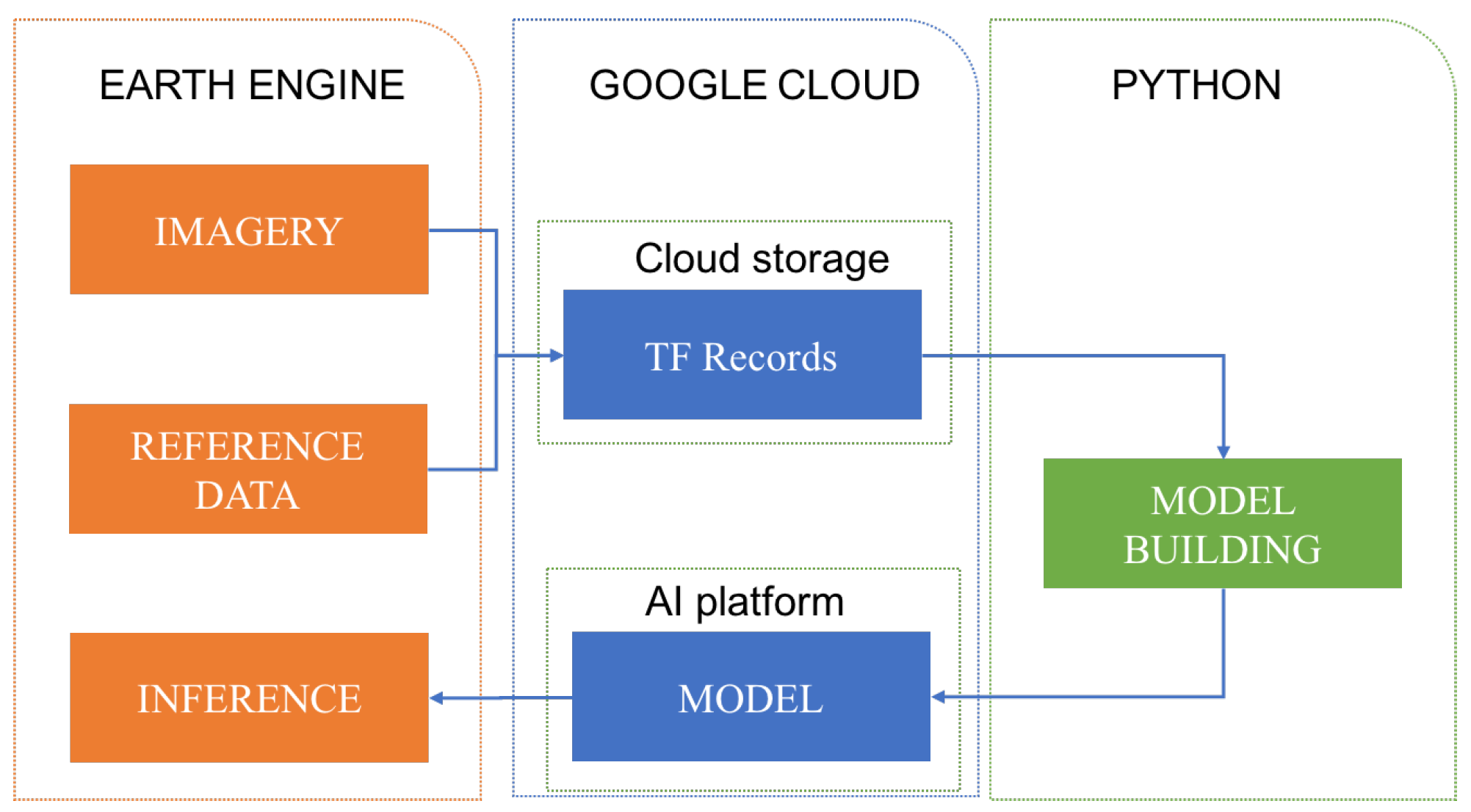
3.1. Modular System
3.2. Proposed System Workflow
3.3. Neural Network Setup
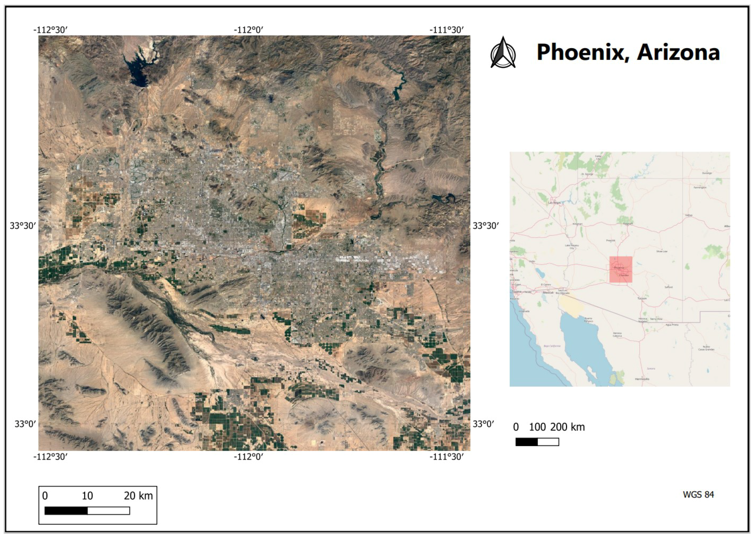
4. Case Study
4.1. Sentinel-2 Data Description
4.2. Sentinel-1 Data Description
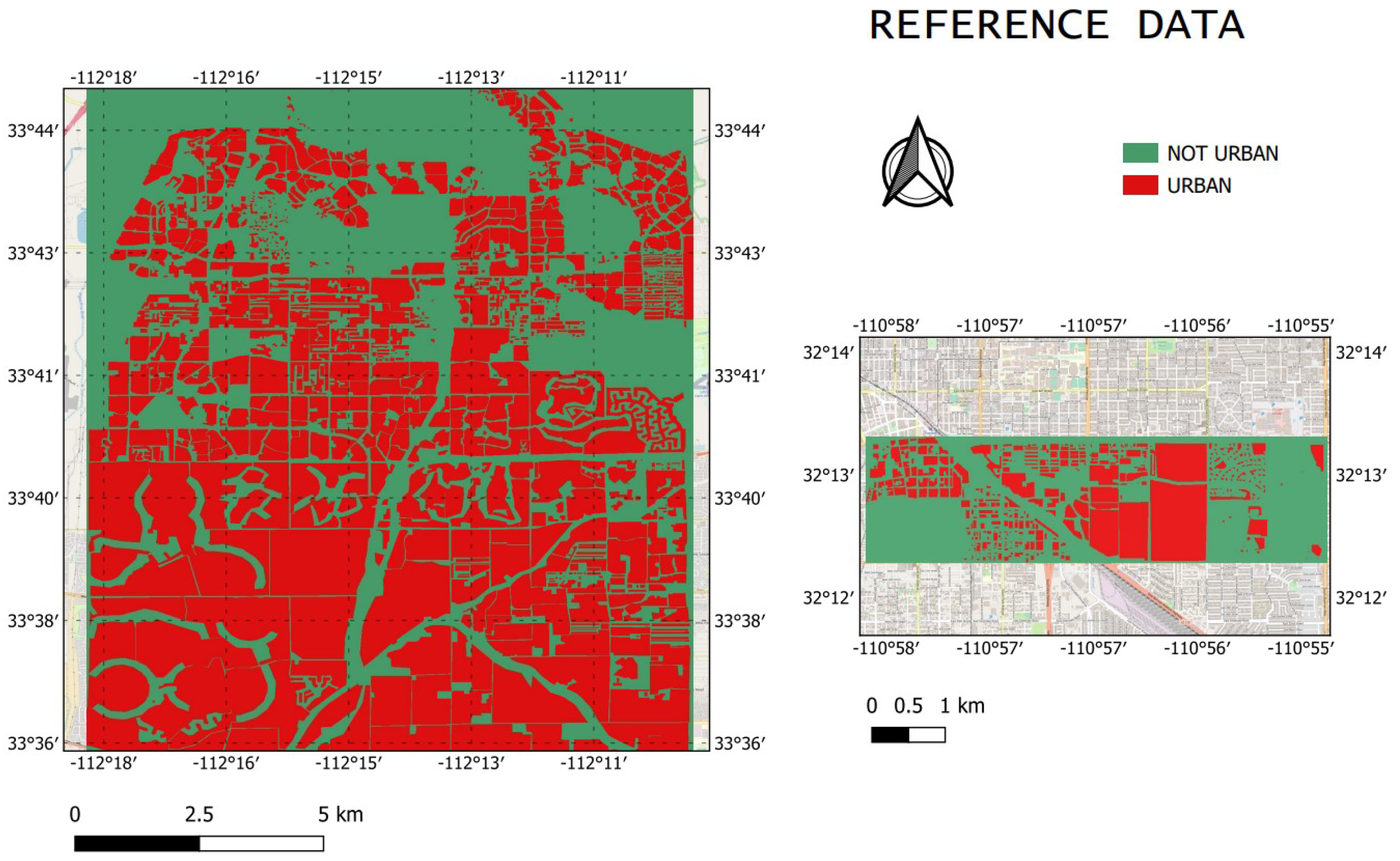
4.3. Preparation of Reference Data
5. Results and Discussion
5.1. Classification Results and Accuracy
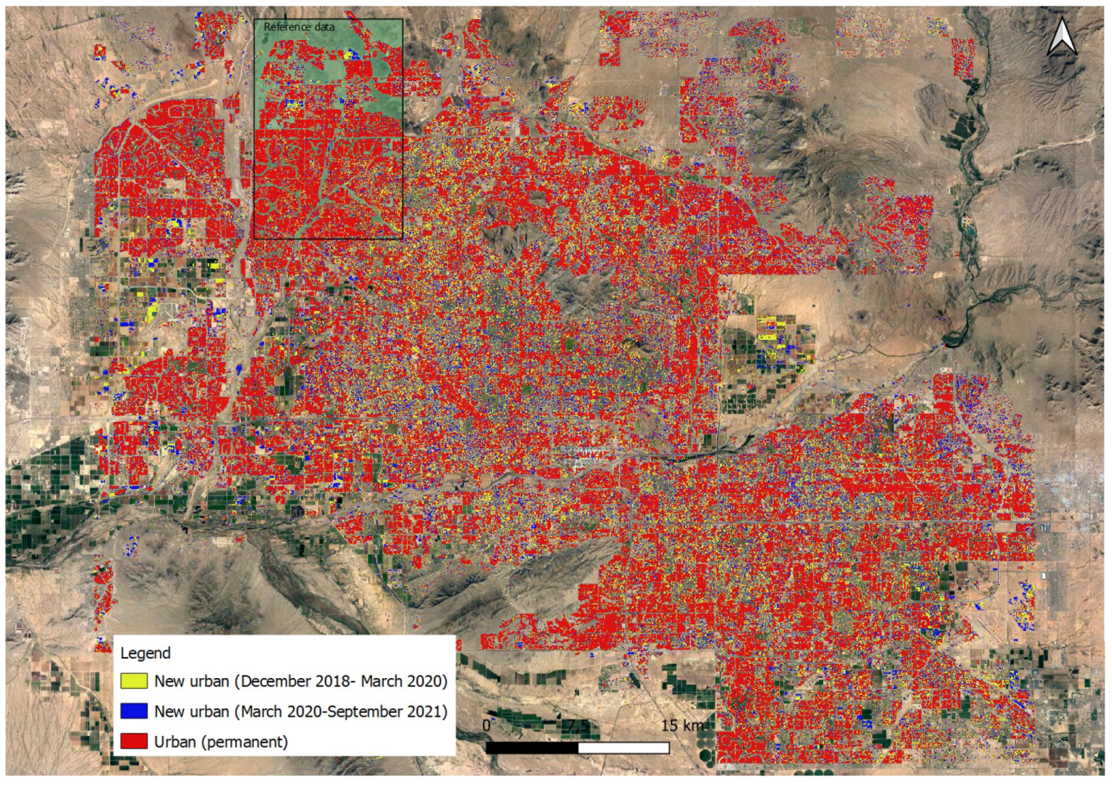
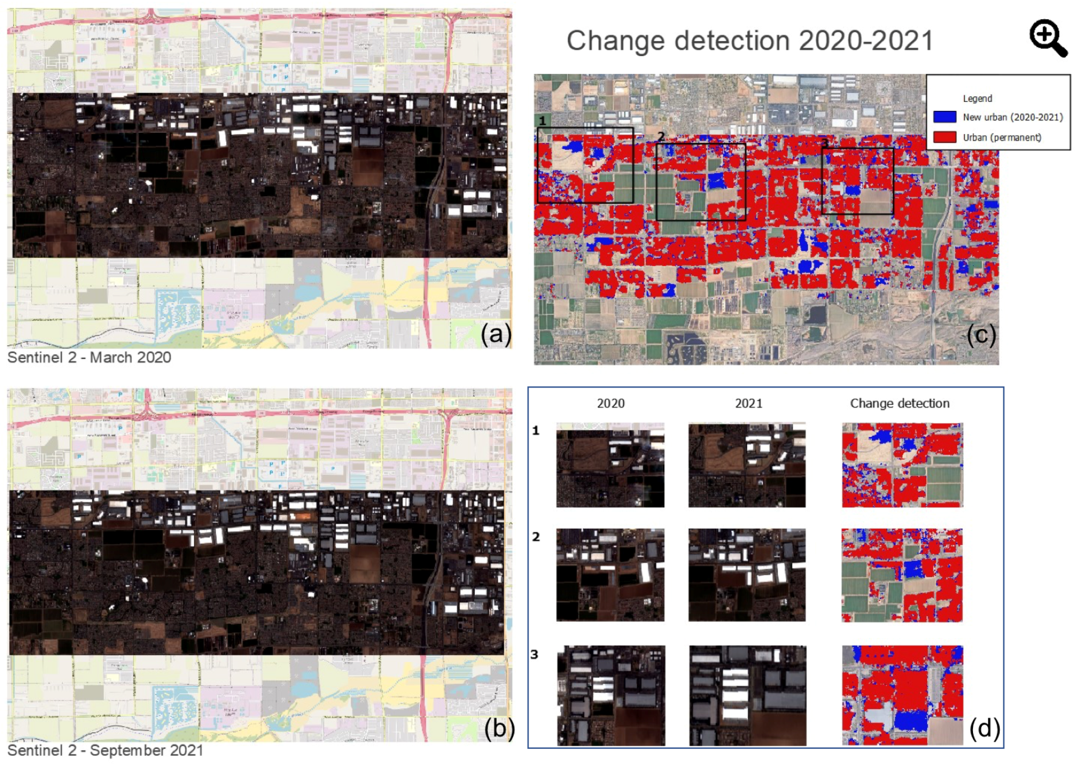
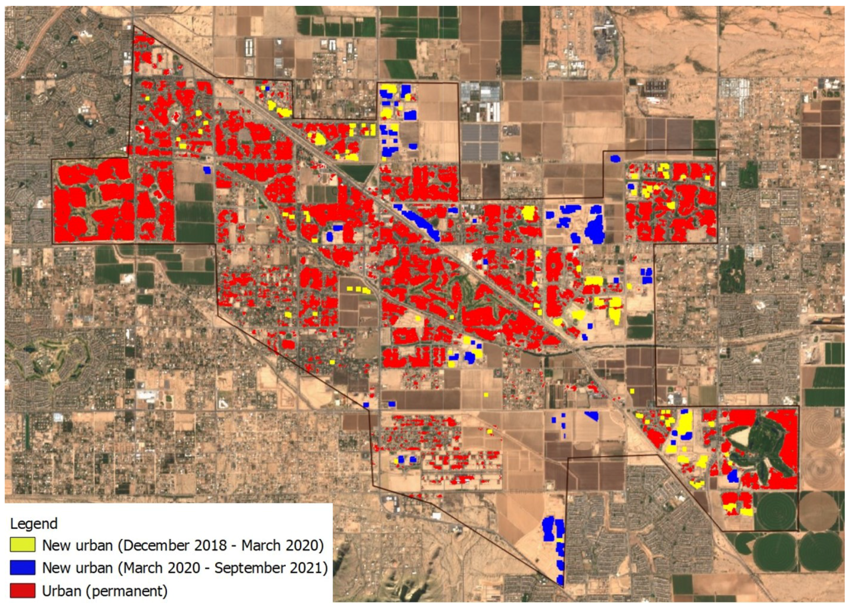
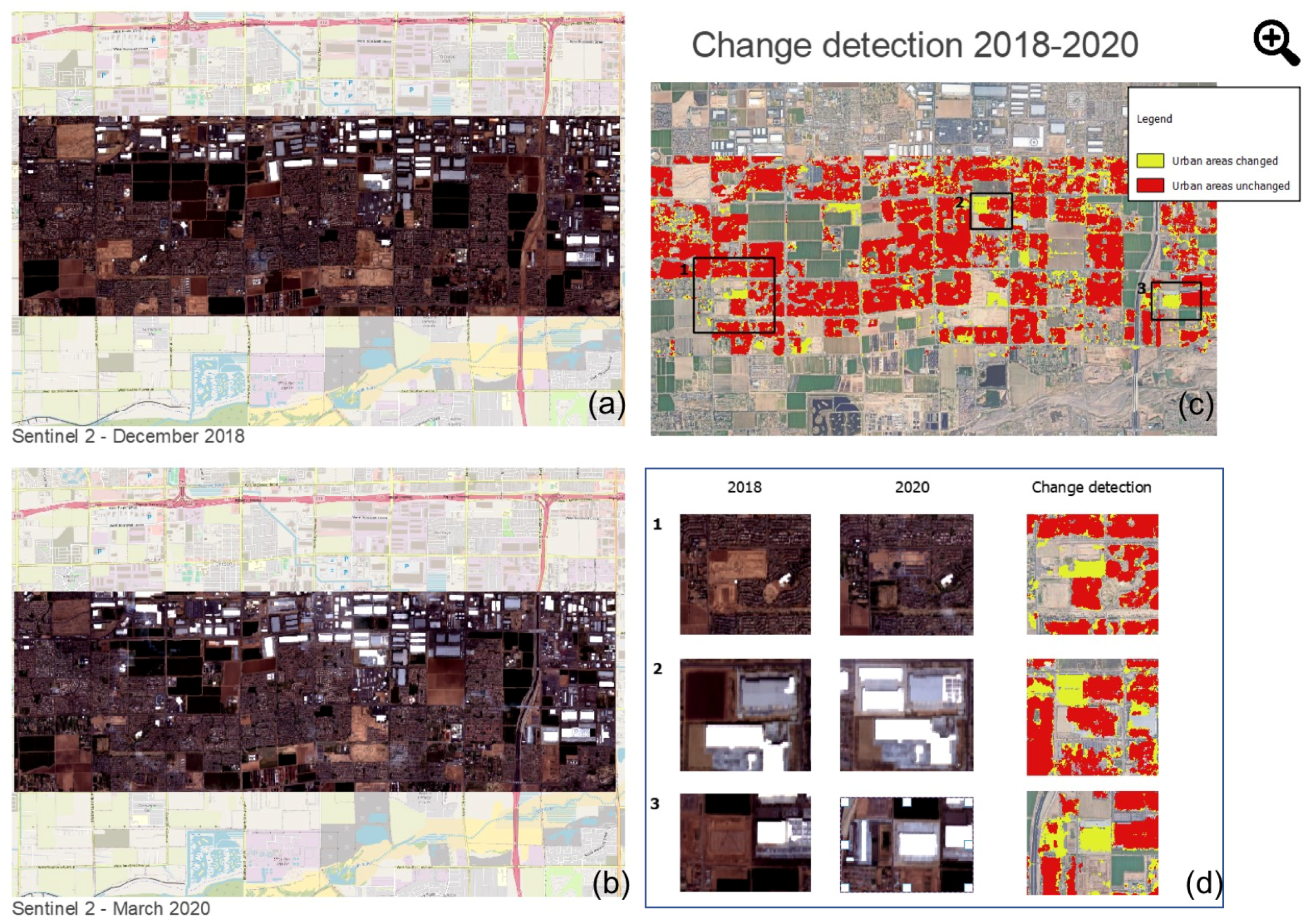
5.2. Urban Sprawl Analysis
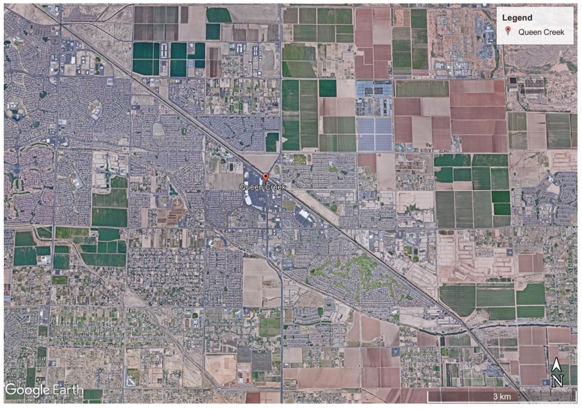
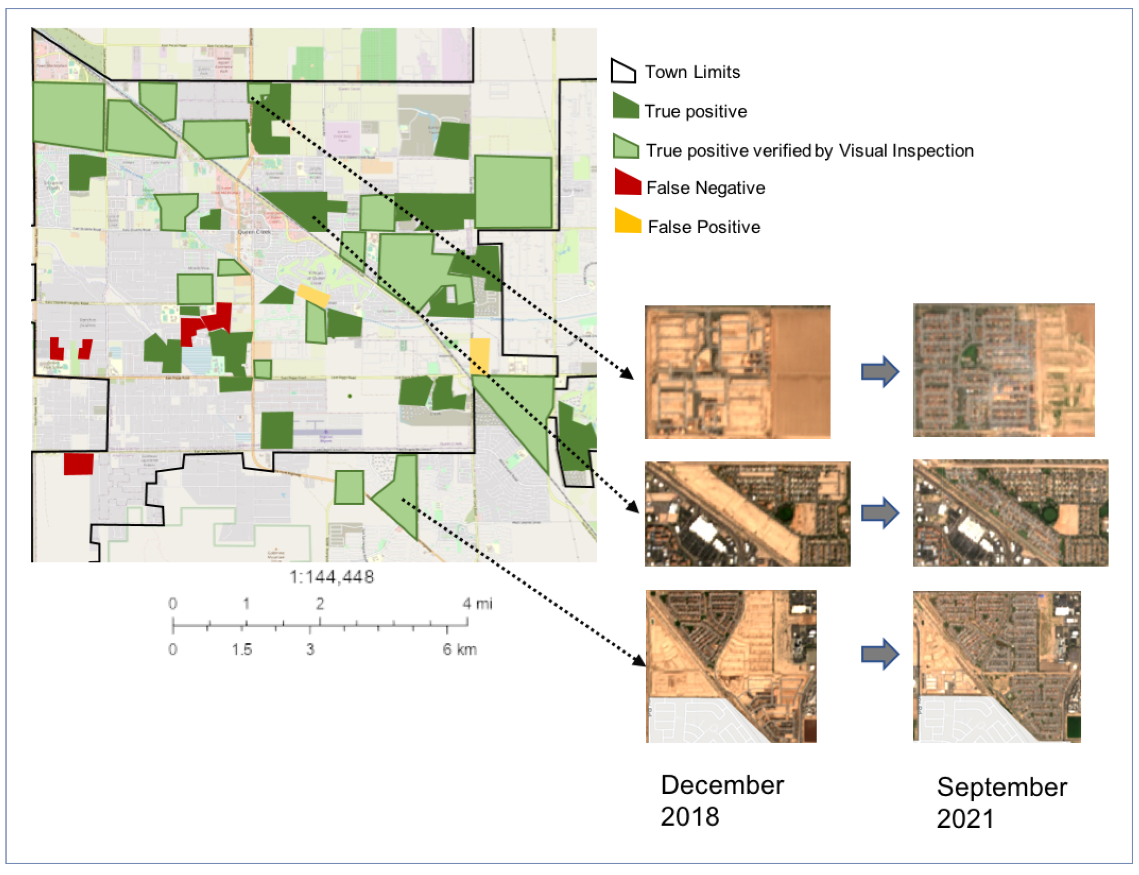
5.3. Validation on Queen Creek
5.4. Consideration of COVID-19 Impact on Urban Growth Rate
6. Conclusions
Author Contributions
Funding
Conflicts of Interest
References
- Nations, U. United Nations Committee of Experts on Global Geospatial Information Management. Available online: https://ggim.un.org/ (accessed on 1 January 2022).
- Kersten, G.E.; Mikolajuk, Z.; Gar-On Yeh, A. Decision Support Systems for Sustainable Development: A Resource Book of Methods and Applications; Springer Science & Business Media: Berlin/Heidelberg, Germany, 2000; pp. 13–27. [Google Scholar] [CrossRef]
- Changnon, S.A. The Great Flood of 1993: Causes, Impacts, and Responses, 1st ed.; Routledge: Abingdon, UK; Taylor and Francis Group: Abingdon, UK, 1996. [Google Scholar] [CrossRef]
- Traver, R. Flood Risk Management: Call for a National Strategy; ASCE Library: Reston, VA, USA, 2014. [Google Scholar] [CrossRef] [Green Version]
- Konrad, C.P. U.S. Geological Survey Fact Sheet 076-03. Available online: https://pubs.usgs.gov/fs/fs07603/ (accessed on 29 November 2016).
- Rees, W.E. Ecological footprints and appropriated carrying capacity: What urban economics leaves out. Environ. Urban. 1992, 4, 121–130. [Google Scholar] [CrossRef]
- Jordan, Y.C.; Ghulam, A.; Chu, M.L. Assessing the Impacts of Future Urban Development Patterns and Climate Changes on Total Suspended Sediment Loading in Surface Waters Using Geoinformatics. J. Environ. Inform. 2014, 24, 65–79. [Google Scholar] [CrossRef] [Green Version]
- Pinto, F. Urban Planning and Climate Change: Adaptation and Mitigation Strategies. TeMA J. Land Use Mobil. Environ. 2014. [CrossRef]
- Cherlet, M.; Hutchinson, C.; Reynolds, J.; Hill, J.S.S.; von Maltitz, G. World Atlas of Desertification; Publication Office of the European Union: Luxembourg, 2018. [Google Scholar]
- Johnson, M.P. Environmental Impacts of Urban Sprawl: A Survey of the Literature and Proposed Research Agenda. Environ. Plan. A Econ. Space 2001, 33, 717–735. [Google Scholar] [CrossRef] [Green Version]
- Alaoui, A.; Ibara, B.O.; Ettaki, B.; Zerouaoui, J. Survey of Process of Data Discovery and Environmental Decision Support Systems. Int. J. Innov. Technol. Explor. Eng. (IJITEE) 2021, 10, 46–50. [Google Scholar] [CrossRef]
- Walling, E.; Vaneeckhaute, C. Developing successful environmental decision support systems: Challenges and best practices. J. Environ. Manag. 2020, 264, 110513. [Google Scholar] [CrossRef]
- Nicola, M.; Alsafi, Z.; Sohrabi, C.; Kerwan, A.; Al-Jabir, A.; Iosifidis, C.; Agha, M.; Agha, R. The socio-economic implications of the coronavirus pandemic (COVID-19): A review. Int. J. Surg. 2020, 78, 185–193. [Google Scholar] [CrossRef]
- Loeffler-Wirth, H.; Schmidt, M.; Binder, H. Covid-19 Transmission Trajectories–Monitoring the Pandemic in the Worldwide Context. Viruses 2020, 12, 777. [Google Scholar] [CrossRef]
- Giordano, G.; Blanchini, F.; Bruno, R.; Colaneri, P.; Di Filippo, A.; Di Matteo, A.; Colaneri, M. Modelling the COVID-19 epidemic and implementation of population-wide interventions in Italy. Nat. Med. 2020, 26, 855–860. [Google Scholar] [CrossRef]
- Sebastianelli, A.; Mauro, F.; Di Cosmo, G.; Passarini, F.; Carminati, M.; Ullo, S.L. AIRSENSE-TO-ACT: A Concept Paper for COVID-19 Countermeasures Based on Artificial Intelligence Algorithms and Multi-Source Data Processing. ISPRS Int. J. Geo-Inf. 2021, 10, 34. [Google Scholar] [CrossRef]
- Ullo, S.L.; Zarro, C.; Wojtowicz, K.; Meoli, G.; Focareta, M. LiDAR-Based System and Optical VHR Data for Building Detection and Mapping. Sensors 2020, 20, 1285. [Google Scholar] [CrossRef] [PubMed] [Green Version]
- Rajendran, G.B.; Kumarasamy, U.M.; Zarro, C.; Divakarachari, P.B.; Ullo, S.L. Land-Use and Land-Cover Classification Using a Human Group-Based Particle Swarm Optimization Algorithm with an LSTM Classifier on Hybrid Pre-Processing Remote-Sensing Images. Remote Sens. 2020, 12, 4135. [Google Scholar] [CrossRef]
- Xu, Y.; Du, B.; Zhang, L.; Cerra, D.; Pato, M.; Carmona, E.; Prasad, S.; Yokoya, N.; Hänsch, R.; Le Saux, B. Advanced Multi-Sensor Optical Remote Sensing for Urban Land Use and Land Cover Classification: Outcome of the 2018 IEEE GRSS Data Fusion Contest. IEEE J. Sel. Top. Appl. Earth Obs. Remote Sens. 2019, 12, 1709–1724. [Google Scholar] [CrossRef]
- Weng, Q.E. Global Urban Monitoring and Assessment through Earth Observation, 1st ed.; CRC Press: Boca Raton, FL, USA, 2014. [Google Scholar] [CrossRef]
- Chien, S.; Tanpipat, V. Remote Sensingremote sensingof Natural Disastersremote sensingof natural disasters. In Encyclopedia of Sustainability Science and Technology; Meyers, R.A., Ed.; Springer: New York, NY, USA, 2012; pp. 8939–8952. [Google Scholar] [CrossRef]
- Pepe, M.; Costantino, D.; Alfio, V.S.; Vozza, G.; Cartellino, E. A Novel Method Based on Deep Learning, GIS and Geomatics Software for Building a 3D City Model from VHR Satellite Stereo Imagery. ISPRS Int. J. Geo-Inf. 2021, 10, 697. [Google Scholar] [CrossRef]
- Temitope Yekeen, S.; Balogun, A.; Wan Yusof, K.B. A novel deep learning instance segmentation model for automated marine oil spill detection. ISPRS J. Photogramm. Remote Sens. 2020, 167, 190–200. [Google Scholar] [CrossRef]
- Li, Q.; Shi, Y.; Auer, S.; Roschlaub, R.; Möst, K.; Schmitt, M.; Glock, C.; Zhu, X. Detection of Undocumented Building Constructions from Official Geodata Using a Convolutional Neural Network. Remote Sens. 2020, 12, 3537. [Google Scholar] [CrossRef]
- Orsomando, F.; Lombardo, P.; Zavagli, M.; Costantini, M. SAR and Optical Data Fusion for Change Detection. In Proceedings of the 2007 Urban Remote Sensing Joint Event, Paris, France, 11–13 April 2007; pp. 1–9. [Google Scholar] [CrossRef]
- Adriano, B.; Yokoya, N.; Xia, J.; Baier, G. Big Earth Observation Data Processing for Disaster Damage Mapping. In Handbook of Big Geospatial Data; Werner, M., Chiang, Y.Y., Eds.; Springer International Publishing: Cham, Switzerland, 2021; pp. 99–118. [Google Scholar] [CrossRef]
- Yang, X.; Lo, C. Using a time series of satellite imagery to detect land use and land cover changes in the Atlanta, Georgia metropolitan area. Int. J. Remote Sens. 2002, 23, 1775–1798. [Google Scholar] [CrossRef]
- Charbonneau, L.; Morin, D.; Royer, A. Analysis of different methods for monitoring the urbanization process. Geocarto Int. 1993, 8, 17–25. [Google Scholar] [CrossRef]
- Yang, X. Urban Remote Sensing: Monitoring, Synthesis and Modeling in the Urban Environment; 2nd ed.; Wiley-Blackwell: Hoboken, NJ, USA, 2021. [Google Scholar] [CrossRef]
- Beneke, C.; Schneider, A.; Sulla-Menashe, D.; Tatem, A.; Tan, B. Detecting change in urban areas at continental scales with MODIS data. Remote Sens. 2015, 158, 331–347. [Google Scholar] [CrossRef]
- Tamiminia, H.; Salehi, B.; Mahdianpari, M.; Quackenbush, L.; Adeli, S.; Brisco, B. Google Earth Engine for geo-big data applications: A meta-analysis and systematic review. ISPRS J. Photogramm. Remote Sens. 2020, 164, 152–170. [Google Scholar] [CrossRef]
- Schmitt, M.; Zhu, X. Data Fusion and Remote Sensing—An Ever-Growing Relationship. IEEE Geosci. Remote Sens. Mag. 2016, 4, 6–23. [Google Scholar] [CrossRef]
- Fatone, L.; Maponi, P.; Zirilli, F. Fusion of SAR/optical images to detect urban areas. In Proceedings of the IEEE/ISPRS Joint Workshop on Remote Sensing and Data Fusion over Urban Areas (Cat. No.01EX482), Rome, Italy, 8–9 November 2001; pp. 217–221. [Google Scholar] [CrossRef]
- Sha, M.; Tian, G. An analysis of spatiotemporal changes of urban landscape pattern in Phoenix metropolitan region. International Conference on Ecological Informatics and Ecosystem Conservation (ISEIS 2010). Procedia Environ. Sci. 2010, 2, 600–604. [Google Scholar] [CrossRef] [Green Version]
- Galletti, C.S.; Myint, S.W. Land-Use Mapping in a Mixed Urban-Agricultural Arid Landscape Using Object-Based Image Analysis: A Case Study from Maricopa, Arizona. Remote Sens. 2014, 6, 6089–6110. [Google Scholar] [CrossRef] [Green Version]
- Li, X.; Myint, S.; Zhang, Y.; Galletti, C.; Zhang, X.; II, B. Object-based land-cover classification for metropolitan Phoenix, Arizona, using aerial photography. Int. J. Appl. Earth Obs. Geoinf. 2014, 33, 321–330. [Google Scholar] [CrossRef]
- Yang, L.; Siddiqi, A.; de Weck, O.L. Urban Roads Network Detection from High Resolution Remote Sensing. In Proceedings of the IGARSS 2019—2019 IEEE International Geoscience and Remote Sensing Symposium, Yokohama, Japan, 28 July–2 August 2019; pp. 7431–7434. [Google Scholar] [CrossRef]
- National Agriculture Imagery Programu. Available online: https://developers.google.com/earth-engine/datasets/catalog/USDA_NAIP_DOQQ (accessed on 1 January 2022).
- Earth Engine Data Catalog. Available online: https://developers.google.com/earth-engine/datasets/catalog (accessed on 1 January 2022).
- Fattore, C.; Abate, N.; Faridani, F.; Masini, N.; Lasaponara, R. Google Earth Engine as Multi-Sensor Open-Source Tool for Supporting the Preservation of Archaeological Areas: The Case Study of Flood and Fire Mapping in Metaponto, Italy. Sensors 2021, 21, 1791. [Google Scholar] [CrossRef]
- Mayer, T.; Poortinga, A.; Bhandari, B.; Nicolau, A.P.; Markert, K.; Thwal, N.S.; Markert, A.; Haag, A.; Kilbride, J.; Chishtie, F.; et al. Deep learning approach for Sentinel-1 surface water mapping leveraging Google Earth Engine. ISPRS Open J. Photogramm. Remote Sens. 2021, 2, 100005. [Google Scholar] [CrossRef]
- Bar, S.; Parida, B.R.; Pandey, A.C. Landsat-8 and Sentinel-2 based Forest fire burn area mapping using machine learning algorithms on GEE cloud platform over Uttarakhand, Western Himalaya. Remote Sens. Appl. Soc. Environ. 2020, 18, 100324. [Google Scholar] [CrossRef]
- Amani, M.; Ghorbanian, A.; Ahmadi, S.A.; Kakooei, M.; Moghimi, A.; Mirmazloumi, S.M.; Moghaddam, S.H.A.; Mahdavi, S.; Ghahremanloo, M.; Parsian, S.; et al. Google Earth Engine Cloud Computing Platform for Remote Sensing Big Data Applications: A Comprehensive Review. IEEE J. Sel. Top. Appl. Earth Obs. Remote Sens. 2020, 13, 5326–5350. [Google Scholar] [CrossRef]
- Poortinga, A.; Thwal, N.S.; Khanal, N.; Mayer, T.; Bhandari, B.; Markert, K.; Nicolau, A.P.; Dilger, J.; Tenneson, K.; Clinton, N.; et al. Mapping sugarcane in Thailand using transfer learning, a lightweight convolutional neural network, NICFI high resolution satellite imagery and Google Earth Engine. ISPRS Open J. Photogramm. Remote Sens. 2021, 1, 100003. [Google Scholar] [CrossRef]
- Google. Tensorflow. Available online: https://www.tensorflow.org/ (accessed on 1 January 2022).
- Ertam, F.; Aydın, G. Data classification with deep learning using Tensorflow. In Proceedings of the 2017 International Conference on Computer Science and Engineering (UBMK), Antalya, Turkey, 5–8 October 2017; pp. 755–758. [Google Scholar] [CrossRef]
- Demirović, D.; Skejić, E.; Šerifović–Trbalić, A. Performance of Some Image Processing Algorithms in Tensorflow. In Proceedings of the 2018 25th International Conference on Systems, Signals and Image Processing (IWSSIP), Maribor, Slovenia, 20–22 June 2018; pp. 1–4. [Google Scholar] [CrossRef]
- Google Earth Engine and Tensorflow. Available online: https://developers.google.com/earth-engine/guides/tensorflow (accessed on 1 January 2022).
- Google Eart Engine and Tensorflow examples. Available online: https://developers.google.com/earth-engine/guides/tf_examples (accessed on 1 January 2022).
- Colaboratory. Available online: https://colab.research.google.com/ (accessed on 1 January 2022).
- Ullo, S.; Del Rosso, M.P.; Sebastianelli, A.; Puglisi, E.; Bernardi, M.; Cimitile, M. How to Develop Your Network with Python and Keras; IET Publishing: London, UK, 2021; pp. 131–158. [Google Scholar] [CrossRef]
- Singhla, R.; Singh, P.; Madaan, R.; Panda, S. Image Classification Using Tensor Flow. In Proceedings of the 2021 International Conference on Artificial Intelligence and Smart Systems (ICAIS), Coimbatore, India, 25–27 March 2021; pp. 398–401. [Google Scholar] [CrossRef]
- Csaybar Website. Available online: https://csaybar.github.io/blog/2019/06/21/eetf2/ (accessed on 1 January 2022).
- Adrian, J.; Sagan, V.; Maimaitijiang, M. Sentinel SAR-optical fusion for crop type mapping using deep learning and Google Earth Engine. ISPRS J. Photogramm. Remote Sens. 2021, 175, 215–235. [Google Scholar] [CrossRef]
- Asma, S.B.; Abdelhamid, D.; Youyou, L. U-Net Based Classification For Urban Areas In Algeria. In Proceedings of the 2020 Mediterranean and Middle-East Geoscience and Remote Sensing Symposium (M2GARSS), Tunis, Tunisia, 9–11 March 2020; pp. 101–104. [Google Scholar] [CrossRef]
- Zhang, W.; Tang, P.; Zhao, L.; Huang, Q. A Comparative Study of U-Nets with Various Convolution Components for Building Extraction. In Proceedings of the 2019 Joint Urban Remote Sensing Event (JURSE), Vannes, France, 22–24 May 2019; pp. 1–4. [Google Scholar] [CrossRef]
- Duan, Y.; Sun, L. Buildings Extraction from Remote Sensing Data Using Deep Learning Method Based on Improved U-Net Network. In Proceedings of the IGARSS 2019—2019 IEEE International Geoscience and Remote Sensing Symposium, Yokohama, Japan, 28 July–2 August 2019; pp. 3959–3961. [Google Scholar] [CrossRef]
- McGlinchy, J.; Johnson, B.; Muller, B.; Joseph, M.; Diaz, J. Application of UNet Fully Convolutional Neural Network to Impervious Surface Segmentation in Urban Environment from High Resolution Satellite Imagery. In Proceedings of the IGARSS 2019—2019 IEEE International Geoscience and Remote Sensing Symposium, Yokohama, Japan, 28 July–2 August 2019; pp. 3915–3918. [Google Scholar] [CrossRef]
- Siddique, N.; Paheding, S.; Elkin, C.P.; Devabhaktuni, V. U-Net and Its Variants for Medical Image Segmentation: A Review of Theory and Applications. IEEE Access 2021, 9, 82031–82057. [Google Scholar] [CrossRef]
- Ronneberger, O.; Fischer, P.; Brox, T. U-Net: Convolutional Networks for Biomedical Image Segmentation. In Proceedings of the International Conference on Medical image computing and computer-assisted intervention (MICCAI), Munich, Germany, 5–9 October 2015. [Google Scholar]
- Sudmanns, M.; Tiede, D.; Lang, S.; Bergstedt, H.; Trost, G.; Augustin, H.; Baraldi, A.; Blaschke, T. Big Earth data: Disruptive changes in Earth observation data management and analysis? Int. J. Digit. Earth 2020, 13, 832–850. [Google Scholar] [CrossRef] [PubMed]
- Sutskever, I.; Martens, J.; Dahl, G.; Hinton, G. On the importance of initialization and momentum in deep learning. In Proceedings of the 30th International Conference on Machine Learning, ICML 2013, Atlanta, GA, USA, 16 June–21 June 2013; pp. 1139–1147. [Google Scholar]
- Government Services. City of Phoenix. Available online: https://www.phoenix.gov/ (accessed on 1 January 2022).
- Phoenix, Arizona. Available online: https://en.wikipedia.org/wiki/Phoenix,_Arizona (accessed on 1 January 2022).
- Taking a Look at Census 2010. City and Town Population Totals: 2010–2019. Available online: https://www.census.gov/data/tables/time-series/demo/popest/2010s-total-cities-and-towns.html (accessed on 1 January 2022).
- Healy, J.; No Large City Grew Faster than Phoenix. The New York Times: Census Updates. Available online: https://www.nytimes.com/2021/08/12/us/phoenix-census-fastest-growing-city.html (accessed on 1 January 2022).
- Martinez, N. Urban Sprawl in Arizona, Commercial Growth and the Effects of It. Available online: https://storymaps.arcgis.com/stories/c51f38e57cc04c35b898e9b30a9dd0d5 (accessed on 12 February 2021).
- Kolankiewicz, L.; Roy Beck, E.A. Population Growth and the Diminishing Natural State of Arizona; NumbersUSA: Arlington County, VA, USA, 2020. [Google Scholar]
- Benedetti, A.; Picchiani, M.; Del Frate, F. Sentinel-1 and Sentinel-2 Data Fusion for Urban Change Detection. In Proceedings of the IGARSS 2018—2018 IEEE International Geoscience and Remote Sensing Symposium, Valencia, Spain, 22–27 July 2018; pp. 1962–1965. [Google Scholar] [CrossRef]
- Hafner, S.; Ban, Y.; Nascetti, A. Exploring the Fusion of Sentinel-1 SAR and Sentinel-2 MSI Data for Built-Up Area Mapping Using Deep Learning. In Proceedings of the 2021 IEEE International Geoscience and Remote Sensing Symposium IGARSS, Brussels, Belgium, 11–16 July 2021; pp. 4720–4723. [Google Scholar] [CrossRef]
- Notarnicola, C.; Asam, S.; Jacob, A.; Marin, C.; Rossi, M.; Stendardi, L. Mountain crop monitoring with multitemporal Sentinel-1 and Sentinel-2 imagery. In Proceedings of the 2017 9th International Workshop on the Analysis of Multitemporal Remote Sensing Images (MultiTemp), Brugge, Belgium, 27–29 June 2017; pp. 1–4. [Google Scholar] [CrossRef]
- Yang, Q.; Wang, L.; Huang, J.; Lu, L.; Li, Y.; Du, Y.; Ling, F. Mapping Plant Diversity Based on Combined SENTINEL-1/2 Data—Opportunities for Subtropical Mountainous Forests. Remote Sens. 2022, 14, 492. [Google Scholar] [CrossRef]
- Gómez, C.; White, J.C.; Wulder, M.A. Optical remotely sensed time series data for land cover classification: A review. ISPRS J. Photogramm. Remote Sens. 2016, 116, 55–72. [Google Scholar] [CrossRef] [Green Version]
- Sentinel 2 Datasets. Available online: https://developers.google.com/earth-engine/datasets/catalog/COPERNICUS_S2_SR (accessed on 1 January 2022).
- Sentinel 1 DATASETS. Available online: https://developers.google.com/earth-engine/datasets/catalog/COPERNICUS_S1_GRD (accessed on 1 January 2022).
- Addabbo, P.; Focareta, M.; Marcuccio, S.; Votto, C.; Ullo, S. Land cover classification and monitoring through multisensor image and data combination. In Proceedings of the 2016 IEEE International Geoscience and Remote Sensing Symposium (IGARSS), Beijing, China, 10–15 July 2016; pp. 902–905. [Google Scholar] [CrossRef]
- Addabbo, P.; Focareta, M.; Marcuccio, S.; Votto, C.; Ullo, S.L. Contribution of Sentinel-2 data for applications in vegetation monitoring. Acta Imeko 2016, 5, 44. [Google Scholar] [CrossRef]
- Mullissa, A.; Vollrath, A.; Odongo-Braun, C.; Slagter, B.; Balling, J.; Gou, Y.; Gorelick, N.; Reiche, J. Sentinel-1 SAR Backscatter Analysis Ready Data Preparation in Google Earth Engine. Remote Sens. 2021, 13, 1954. [Google Scholar] [CrossRef]
- Ghorbanian, A.; Zaghian, S.; Asiyabi, R.M.; Amani, M.; Mohammadzadeh, A.; Jamali, S. Mangrove Ecosystem Mapping Using Sentinel-1 and Sentinel-2 Satellite Images and Random Forest Algorithm in Google Earth Engine. Remote Sens. 2021, 13, 2565. [Google Scholar] [CrossRef]
- Google Earth Engine and Sentinel pre-processing. Available online: https://developers.google.com/earth-engine/guides/sentinel1#sentinel-1-preprocessing (accessed on 1 January 2022).
- Zarro, C. Ground Truth of Phoenix. Available online: https://code.earthengine.google.com/?asset=users/chiarazarro/GroundTruthPHOENIX (accessed on 1 January 2022).
- Zarro, C. Ground Truth of Tucson. Available online: https://code.earthengine.google.com/?asset=users/chiarazarro/GroundTruthTUCSON (accessed on 1 January 2022).
- Administration, Q.C. Queen Creek Development Map. Available online: https://qcgis.maps.arcgis.com/apps/View/index.html?appid=69f33e00224d4ad78c462be9f412d628 (accessed on 29 November 2016.).
- National Association of Home Builders. Building Permits by State and Metro Area. Available online: https://www.nahb.org/news-and-economics/housing-economics/state-and-local-data/building-permits-by-state-and-metro-area (accessed on 17 February 2022).
- Bureau, U.S.C. Pandemic Population Change across Metro America: Accelerated Migration, Less Immigration, Fewer Births and More Deaths. Available online: https://www.brookings.edu/research/pandemic-population-change-across-metro-america-accelerated-migration-less-immigration-fewer-births-and-more-deaths/ (accessed on 20 May 2021).


| S2 | S2 and S1 | S2 and S1_ARD | |
|---|---|---|---|
| Precision | 0.703 | 0.746 | 0.705 |
| Recall | 0.811 | 0.806 | 0.823 |
| F1 score | 0.754 | 0.775 | 0.759 |
Publisher’s Note: MDPI stays neutral with regard to jurisdictional claims in published maps and institutional affiliations. |
© 2022 by the authors. Licensee MDPI, Basel, Switzerland. This article is an open access article distributed under the terms and conditions of the Creative Commons Attribution (CC BY) license (https://creativecommons.org/licenses/by/4.0/).
Share and Cite
Zarro, C.; Cerra, D.; Auer, S.; Ullo, S.L.; Reinartz, P. Urban Sprawl and COVID-19 Impact Analysis by Integrating Deep Learning with Google Earth Engine. Remote Sens. 2022, 14, 2038. https://doi.org/10.3390/rs14092038
Zarro C, Cerra D, Auer S, Ullo SL, Reinartz P. Urban Sprawl and COVID-19 Impact Analysis by Integrating Deep Learning with Google Earth Engine. Remote Sensing. 2022; 14(9):2038. https://doi.org/10.3390/rs14092038
Chicago/Turabian StyleZarro, Chiara, Daniele Cerra, Stefan Auer, Silvia Liberata Ullo, and Peter Reinartz. 2022. "Urban Sprawl and COVID-19 Impact Analysis by Integrating Deep Learning with Google Earth Engine" Remote Sensing 14, no. 9: 2038. https://doi.org/10.3390/rs14092038
APA StyleZarro, C., Cerra, D., Auer, S., Ullo, S. L., & Reinartz, P. (2022). Urban Sprawl and COVID-19 Impact Analysis by Integrating Deep Learning with Google Earth Engine. Remote Sensing, 14(9), 2038. https://doi.org/10.3390/rs14092038