Fusion of a Static and Dynamic Convolutional Neural Network for Multiview 3D Point Cloud Classification

Abstract

Three-dimensional (3D) point cloud classification methods based on deep learning have good classification performance; however, they adapt poorly to diverse datasets and their classification accuracy must be improved. Therefore, FSDCNet, a neural network model based on the fusion of static and dynamic convolution, is proposed and applied for multiview 3D point cloud classification in this paper. FSDCNet devises a view selection method with fixed and random viewpoints, which effectively avoids the overfitting caused by the traditional fixed viewpoint. A local feature extraction operator of dynamic and static convolution adaptive weight fusion was designed to improve the model’s adaptability to different types of datasets. To address the problems of large parameters and high computational complexity associated with the current methods of dynamic convolution, a lightweight and adaptive dynamic convolution operator was developed. In addition, FSDCNet builds a global attention pooling, integrating the most crucial information on different view features to the greatest extent. Due to these characteristics, FSDCNet is more adaptable, can extract more fine-grained detailed information, and can improve the classification accuracy of point cloud data. The proposed method was applied to the ModelNet40 and Sydney Urban Objects datasets. In these experiments, FSDCNet outperformed its counterparts, achieving state-of-the-art point cloud classification accuracy. For the ModelNet40 dataset, the overall accuracy (OA) and average accuracy (AA) of FSDCNet in a single view reached 93.8% and 91.2%, respectively, which were superior to those values for many other methods using 6 and 12 views. FSDCNet obtained the best results for 6 and 12 views, achieving 94.6%, 93.3%, 95.3%, and 93.6% in OA and AA metrics, respectively. For the Sydney Urban Objects dataset, FSDCNet achieved an OA and F1 score of 81.2% and 80.1% in a single view, respectively, which were higher than most of the compared methods. In 6 and 12 views, FSDCNet reached an OA of 85.3% and 83.6% and an F1 score of 85.5% and 83.7%, respectively.

1. Introduction

With the rapid development of artificial intelligence and deep learning technology, breakthroughs have been made in 3D perception and understanding; one such breakthrough, the point cloud, contains abundant geometric, shape, and structure information. The 3D point cloud is mainly collected by light detection and ranging (LiDAR) scanner, red, green, blue, and depth (RGB-D) camera, and other sensor equipment or obtained by model conversion using computer software, as shown in Figure 1. It is widely used in several fields, such as urban environment monitoring [1], urban form analysis [2], autonomous driving [3,4], computer vision [5,6], robotics [7], and reverse engineering modeling [8]. Research fields related to the 3D point cloud include registration, denoising, classification, target detection, and segmentation. Among these fields, the classification-based 3D point cloud is one of the most basic and significant. Hence, most research focuses on improving the accuracy and efficiency of classification-based point clouds [9,10,11,12,13,14,15].

Classification methods based on the 3D point cloud include voxel, direct point cloud, and multiview methods, which are the subject of much research.

1.1. Voxel-Based

Voxels, i.e., volume pixels, represent a 3D region with a constant scalar or vector [16]. Because voxels can represent complex objects with simplified and discrete units, such as particles, they have powerful capabilities in simulating the behavior of complex objects in the real world, while their structural representation is relatively simple. Plaza et al. [17] proposed a voxel-based 3D point cloud data classification method for natural environments that uses a multilayer perceptron (MLP) to conduct a statistical geometric analysis on the spatial distribution of internal points and voxel classification. The local spatial distribution characteristics around points are defined by the principal components of the point position covariance matrix. The combination of voxels and neural networks realizes faster computing speeds than other strategies; however, it does not remedy the essential shortcomings of voxels themselves, including intensive computation and time consumption. Liu et al. [18] presented a convolutional neural network (CNN) model, point-voxel, that captures the overall structure and details of an object with two modules, integrating the advantages of a point cloud and a grid. It has less data overhead, better data regularity, and a lower memory consumption than other voxel models, as well as better classification accuracy than many voxel-based models; however, it still has the low efficiency and intrinsic stereotype of voxel convolution and the combination of voxels and a point cloud. Plaza et al. [19] proposed a general framework based on a voxel neighborhood, which was compared to different supervised learning classifiers. The framework uses simple features in the support region that are defined based on the voxel itself, and it assigns each non-overlapping voxel point in the regular grid to the same class, which improves the effectiveness of 3D space shape feature classification. Therefore, it is easier to reduce processing time and parallelize. Preliminary experiments have been conducted, and further analysis is required using diverse performance indicators, environments, and sensors. Liu et al. [20] proposed a generalized learning network based on voxels—VB-Net—and used it to classify 3D objects. By transforming the original point cloud to voxels, VB-Net can be used to extract features for the target classification of a generalized learning system. The technique significantly reduces the time required for system training, although the classification accuracy must be improved. In particular, with an increase in 3D object resolution, the classification accuracy decreases sharply. Hamada et al. [21] considered the change in voxel density along the depth direction and presented a 3D scene classification measure based on three-projection voxel expansion, which normalizes the scene according to the position and size and projects it onto three vertical planes. The algorithm applies deep learning to predict the category of each scene, combining three images, and greatly improves classification accuracy. However, three-projection voxel expansion must be standardized to make each 3D scene suitable for voxels. Apparently, if the 3D scene is large enough, then tri-projection voxel splatting (TVS) may not recognize small objects. Wang et al. [22] proposed a voxel-based CNN, NormalNet, that employs a reflection convolution concatenation (RCC) series module as a convolution layer to extract distinguishable features via a relatively good reflection number for 3D visual tasks, which significantly reduces the number of parameters and enhances network performance. Nevertheless, the model could still be further optimized since the best reflection number was not found in the key module RCC. Hui et al. [23] explored the unsuitability of binary voxels for 3D convolution representation. By assigning distance values to voxels, they improved the accuracy by about 30% and designed a fast, full connection and convolution hybrid cascade network for the classification of 3D objects. Its average reasoning time is faster than that of methods based on a point cloud and voxels, and its accuracy is also higher; however, the recognition rate of some hard samples (some sample data that take a high price to train and learn, yet usually obtain a large loss value and worse performance) in the deep network is lower than that of its shallow counterpart. Voxel-based classification has the disadvantage of a high storage overhead, and processing a large, complicated 3D image represented by direct voxels in 3D convolution requires significant graphics processing unit (GPU) resources and considerable computing time. This problem can be solved by reducing the resolution of the 3D image; however, this will decrease the accuracy of the final trained model.

1.2. Point Cloud-Based

A point cloud is a collection of data points defined by a coordinate system. Each point contains abundant information, including 3D coordinates (x, y, z), color, classification value, intensity, and time. This representation form has the characteristics of disorder, sparsity, rotation, and translation invariance. Compared with voxel methods, point cloud-based processing discards additional model transformations and directly considers the original point cloud as the processing object, which can reduce storage. Qi et al. [10] designed PointNet, a neural network that directly trains point clouds using a learned T-Net transformation matrix to ensure invariance in the specific spatial transformation and extract the features of point cloud data through an MLP. The final global features are obtained by maximum pooling for features in each dimension and sent to the MLP for the classification of 3D objects. Since the point cloud operates directly without complex preprocessing, the network architecture is efficient, and it resists disturbance. Yet, the network does not learn the connection among local points; hence, the model cannot capture information on local features. Zhao et al. [24] proposed a deep neural network that combines multiscale features with PointNet, adopting multiscale approaches to extract the neighborhood features of points and combining them with global features extracted by PointNet to classify LiDAR point clouds. The network has a good classification effect; however, it extracts local features with poor efficiency. Li et al. [25] proposed an optimization method based on PointNet to improve the accuracy of 3D classification models. The model can obtain more abstract features by increasing the number of hidden layers and can generate discriminant features by combining the Softmax and central loss functions. The improved model has better performance than the original PointNet. Nevertheless, it has not been studied in detail whether a more lightweight deep convolution network can be used to further optimize the model. Aiming to solve the occlusion problem of environment classification using a 1D signal and two-dimensional (2D) image, Zhang et al. [26] proposed directional PointNet to directly classify a 3D point cloud. The model utilizes the direction information of a point cloud to classify terrain in order to help wearable robot objects walk in complex environments. It provides a robust and efficient classification of the environment; however, its high classification accuracy is limited to specific application fields, and the generalization effect warrants further exploration. Because a PointNet network is unable to capture the local structure generated by metric space points, its capability to identify fine-grained patterns and generalize complex scenes is limited. The PointNet++ hierarchical network model [11] was proposed to improve PointNet. The PointNet++ architecture adaptively combines multiscale features through a learning layer and combines the local point set density to effectively learn the point set features at a deep level for more accurate classification. The time consumption is greatly increased compared to PointNet, especially in preprocessing. Rivlin et al. [27] used 3D coordinates as class identifiers by comparing the attributes of shape moments and added a polynomial function of coordinates to accommodate higher-order shape moments. Their experiments demonstrated its improved memory usage and computational complexity; it was also able to classify rigid objects. However, this method has not been applied for use in other fields involving geometric analysis. Yang et al. [28] replaced the expensive multi-head attention mechanism with parameter-efficient group shuffle attention (GSA) to develop a converter of point attention that can process input data of different sizes and exhibits equivalence of transformation. Gumble subset sampling (GSS) was proposed for end-to-end learning and task-agnostic sampling. By selecting subsets in the representative hierarchy, the network can obtain a stronger representation of the input set at a lower computational cost. Experiments revealed the effectiveness and efficiency of the method in 3D image classification; however, GSS was not applied to general datasets, and its effectiveness and interpretability in hierarchical multi-instance learning were not explored. Zhao et al. [29] presented PointWeb to extract context features from a local neighborhood in the point cloud; PointWeb closely connects each point and uses an adaptive feature adjustment module to find the interaction among points. This framework can better learn the point representation for point cloud processing; however, its application to the understanding of 3D scenes needs further verification. Xie et al. [30] proposed a generation model of a disordered point cloud, where an energy function learns the coordinate coding of each point and then aggregates all individual point features into the energy of the whole point cloud. The model is trained by maximum likelihood learning based on Markov chain Monte Carlo (MCMC) and its variants, without an auxiliary network, and does not rely on the manual drawing of distance measurements to generate the point cloud. Thus, it is an efficient method for point cloud classification. However, the disturbance rejection of the model and the processing of point clouds with many outliers are unsatisfactory in practical applications. Yan et al. [31] proposed an end-to-end network called point adaptive sampling and local and nonlocal module (PointASNL) for robust point cloud processing in the presence of outliers and noise in the original point cloud. The network includes an adaptive sampling module and a local and nonlocal module. The first module adopts farthest point sampling (FPS) to sample the initial point cloud and reweights the neighborhood value, while the second captures neighborhood points and long-range dependencies. PointASNL has achieved a high level of robustness in point cloud classification; however, the fine-tuning strategy in the adaptive sampling module requires constant exploration. In the task of point cloud classification and segmentation, it is difficult to use geometric information to extract local features and correctly select important features. Accordingly, Jin et al. [32] proposed a graph-based neural network with an attention pooling strategy, named AGNet, which can effectively extract the spatial information of different distances and select the most crucial features, achieving a good classification and segmentation effect. Because of the influence of sensors, scenes, and other factors, the sparsity of collected point clouds in real environments is much different, which affects the accuracy of the final classification. Hence, complex preprocessing on point clouds is inevitable. Moreover, disturbances and outliers will inevitably appear in a real point cloud, i.e., a point may appear in a radius near its sampled area or anywhere in space and rotating the point cloud will represent the same 3D object with a different shape. Therefore, point cloud outliers and disturbances, as well as rigid transformation processing, make point cloud-based 3D object classification more intricate.

1.3. Multiview-Based

Multiview-based 3D point cloud classification involves the collection of 2D images of a 3D point cloud object from different viewpoints, which are sent to a CNN model for classification to produce the final representation. Chen et al. [4] studied 3D high-precision target detection in autonomous driving scenes and proposed a multiview 3D network consisting of sub-networks for 3D object representation and multiview feature fusion. Its deep fusion scheme combines regional features from multiple views, enabling the middle layers of different paths to interact. This improves the accuracy of the classification and reduces the amount of calculation. However, because the model utilizes a region-based fusion network, it is deficient in the extraction of feature information of objects from a global point of view. Using a large-scale ground truth dataset and a baseline view-based recognition method, Papadakis et al. [33] benchmarked multiple multiview hypothesis fusion schemes under various environmental assumptions and observation capabilities. Their experimental results highlighted significant aspects that should be considered in the design of a multiview-based recognition pipeline, while the analysis was only reflected in the 3D shape without considering texture characteristics. Cheng et al. [34] proposed a feature selection method that embeds low-rank constraints, sparse representation, and global and local structure learning in a unified framework; constructs a Laplace matrix based on the regularization term of a hypergraph; and applies a novel optimization algorithm to solve the objective function. The method achieves good classification performance on multiview datasets but does not extend to unsupervised and clustering learning. Inspired by the singular multiview convolution network structure, Pramerdorfer et al. [35] proposed a 3D bounding box approach that combines jointly classified objects and regression models in a depth map. This method has excellent robustness to occlusion. It can process the views of encoded object geometry and occlusion information to output class scores and bounding box coordinates in world coordinates without post-processing. The model has excellent classification accuracy and a low regression error rate. It is worth researching whether its performance can be improved with different front-end architectures, such as ResNet, or by integrating the model into a deployed detection system based on Kinect to evaluate its performance. Feng et al. [12] presented a group view convolution neural network (GVCNN) for discriminative 3D shape description and hierarchical correlation modeling to better utilize the inherent hierarchical correlation and resolution between multiple views. This method introduces a hierarchical shape description framework, including views, groups, and shape level descriptors; considers the correlation among the views of each shape; and uses the group information for shape representation. It has realized performance improvements in 3D shape classification and retrieval tasks; however, it is not perfect with more complete views. Liu et al. [36] proposed a multiview hierarchical fusion network (MVHFN) that includes visual feature learning and multiview hierarchical fusion modules. In the first module, a 2D CNN extracts the visual features of multiple views drawn around a 3D object, while multiple view features are integrated as a compact descriptor in the second module. The model can find discriminant content by learning the cluster-level feature information, making full use of multiview and improving the classification accuracy. However, the number of views captured is low and the order of views is fixed, which cannot simulate ground object recognition in real 3D scenes well. Li et al. [37] proposed a probabilistic hierarchical model for multiview classification that learns a potential variable to fuse multiple features obtained from the same view, sensor, and morphology; applies the mapping matrix of a view to project the potential variable from the shared space to multiple observations; and employs expectation maximization (EM) to estimate parameters and potential variables. The network model can integrate multiview and feature data in multilevel, and the calculation of relevant parameters is repeatable and in line with common sense; however, the complexity of the model is high and its calculations are inefficient. He et al. [38] presented an online Bayesian multiview learning algorithm that learns the prediction subspace based on the principle of maximum margin, defines the potential marginal loss, and minimizes the learning problems associated with various Bayesian frameworks by using the theory of pseudo-likelihood and data enhancement. It obtains an approximate a posteriori change according to past samples. The model can attain higher classification performance than some advanced methods and can automatically infer weights and penalty parameters; however, the calculation is complex when the dataset is large. Li et al. [39] designed a Gaussian process latent variable model (GPVLM), which represents multiple views in a common subspace. It learns another projection from observed data to shared variables through view sharing and view-specific kernel parameters under a Gaussian process structure. Potential variables are changed to label information by Gaussian transformation, which reveals the correlation between views, and the model performs relatively well. Nevertheless, the radial basis function (RBF) cannot adapt to distributed and complex data, and multi-core learning is not considered. Yu et al. [40] proposed latent multiview CNN (LMVCNN), which utilizes predefined or random multiview images to identify 3D shapes and consists of three sub-convolution neural networks. The three CNN modules generate a multi-category probability distribution, build a potential vector to help the first CNN select the appropriate distribution, and output the category probability distribution of one view from another. LMVCNN has good discriminative ability for predefined and random views and can show excellent performance when the number of views is small; however, it does not solve the problem of 3D shape recognition without background interference. Hence, it is difficult to recognize objects in real 3D environments. Considering similarity measurements between image blocks, Yu et al. [13] proposed a multiview harmonized bilinear network (MHBN) for 3D object recognition. The model applies bilinear pooling to local convolution to obtain a compact global representation and produces a more discriminant representation by coordinating the singular values of set features. Its effectiveness in 3D object recognition was verified by experiments, where a high classification accuracy was achieved. Traditional methods invariably have certain disadvantages, such as multiview selection from a fixed viewpoint and static convolution for feature extraction. Therefore, if these disadvantages are overcome, the classification accuracy can be further improved. Multiview-based methods occupy less storage space than voxel and direct point cloud processing because they only require several 2D views. Converted 2D views can be adequately utilized by the current 2D CNN model; thus, training time is significantly reduced and the accuracy of model classification is the highest among the three different methods described above, namely voxel, point cloud, and multiview-based techniques.

However, most multiview-based methods [9,12,13] use traditional fixed-view projection when converting a 3D point cloud to 2D views, which can cause high similarity among view data. Therefore, the discriminative ability of the model decreases with multiple views on a test set, thus reducing the generalization ability of the model. Moreover, these methods often use a pretrained CNN backbone model to improve the efficiency of feature extraction; however, most backbone models adopt traditional static convolution, which is not adaptive to different data. Additionally, the use of only maximum and average pooling in feature fusion causes a considerable loss of detail and makes fusion inefficient. In order to solve these problems, we propose FSDCNet, a fusion of static and dynamic convolution networks for 3D point cloud classification with high accuracy, high efficiency, and a strong generalization ability. The model has five advantages over the abovementioned deep learning-based methods:

(1)

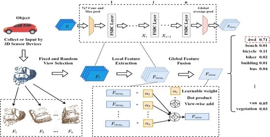
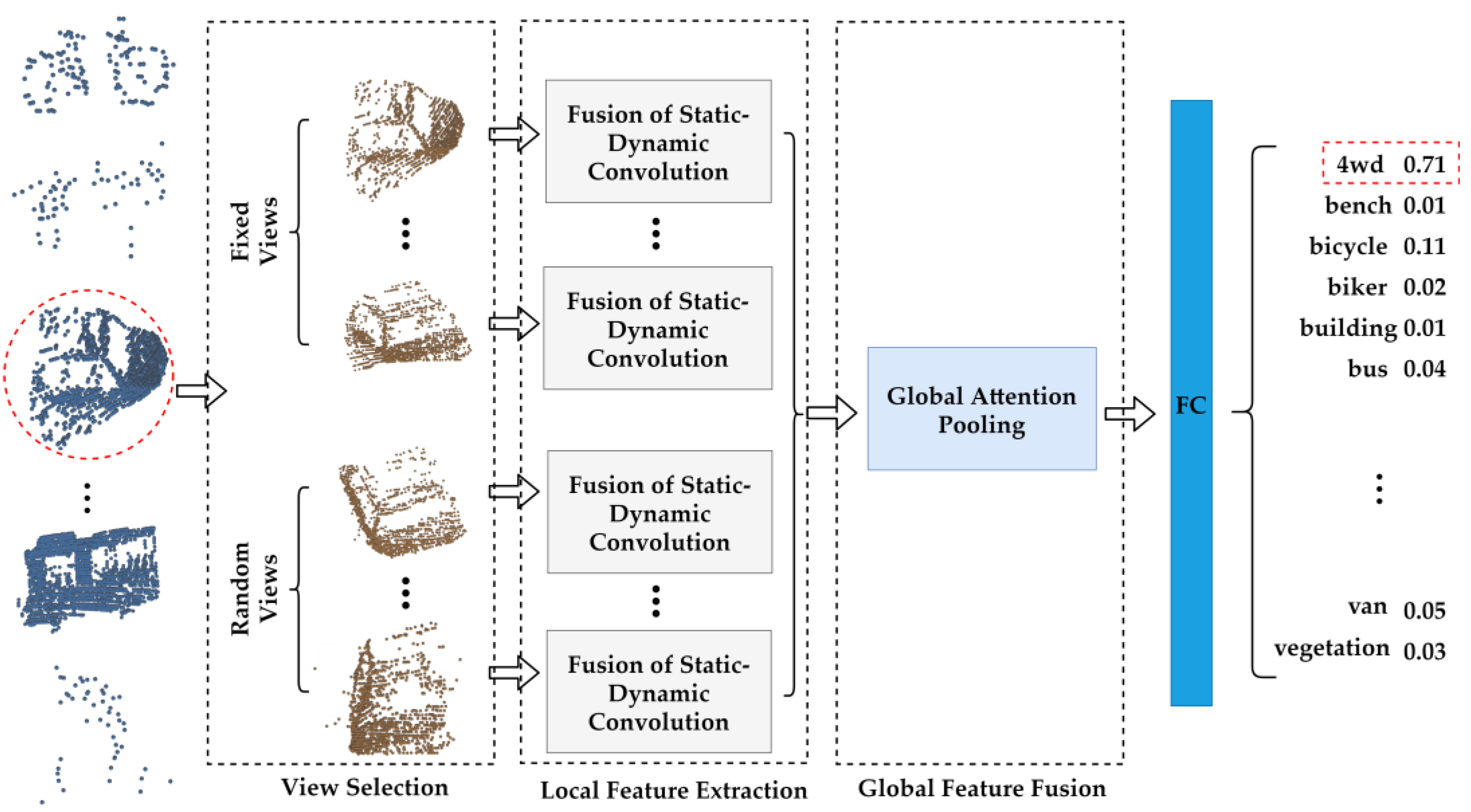
FSDCNet, a fusion static and dynamic convolution neural network, is proposed and applied to the classification of a 3D point cloud. The network adopts fixed and random viewpoint selection method for multiview generation. Meanwhile, it carries out local feature extraction by combining lightweight dynamic convolution with traditional static convolution in parallel. In addition, adaptive global attention pooling is used for global feature fusion. The network model is applicable not only to dense point clouds (ModelNet40), but also to sparse point clouds (Sydney Urban Objects). Our experiments demonstrate that it can achieve state-of-the-art classification accuracy on two datasets. Our algorithm framework, FSDCNet, is evidently different from other advanced algorithm frameworks.

(2)

FSDCNet devises a view selection method of fixed and random viewpoints in the process of converting a point cloud into a multiview representation. The combination of random viewpoints avoids the problem of high similarity among views obtained by the traditional fixed viewpoint and improves the generalization of the model.

(3)

FSDCNet constructs a lightweight dynamic convolution operator. The operator solves the problems of large parameters and expensive computational complexity in dynamic convolution, while maintaining the advantages of dynamic convolution; the complexity is only equivalent to that of traditional static convolution. Meanwhile, it can obtain abundant feature information in different receptive fields.

(4)

FSDCNet proposes an adaptive fusion method of static and dynamic convolution. It can solve the problem of weak adaptability associated with traditional static convolution and extract more fine-grained feature information, which significantly improves the performance of the network model.

(5)

FSDCNet designs adaptive global attention pooling to avert the low efficiency of global feature fusion with maximum and average pooling. It can integrate the most crucial details on multiple local views and improve the fusion efficiency of multiview features.

The remainder of this paper is organized as follows. The FSDCNet network framework is introduced in Section 2. Section 3 describes the datasets and the experimental environment, compares FSDCNet with other point cloud classification algorithm models using multiple metrics, and presents the experimental results and analysis. Section 4 summarizes the paper and proposes future work.

2. Methods

The point clouds obtained in various approaches were used as the input of our FSDCNet model to obtain the final 3D point cloud classification results. Our FSDCNet framework is shown in Figure 2. It has three parts: (a) preprocess the original point cloud, convert it into 2D views through fixed and random viewpoints, and combine them in a specific proportion (Section 2.1); (b) for these preprocessed 2D views, a lightweight dynamic convolution and traditional static convolution work in parallel to form a local operator for point cloud feature extraction, thereby improving the model’s efficiency (Section 2.2); and (c) for higher classification accuracy, apply influence weights to view features in the process of fusion to global features using attention pooling (Section 2.3).

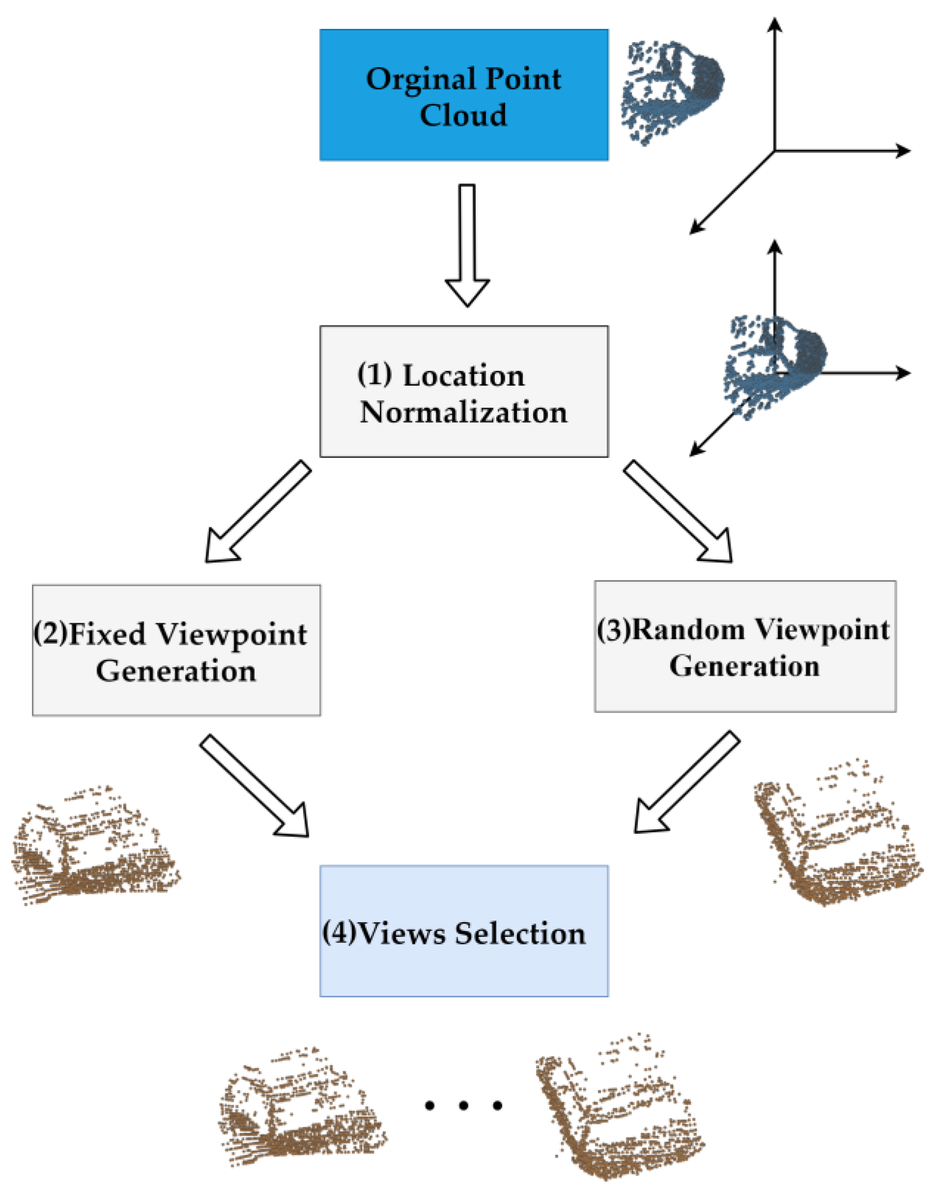
2.1. Multiview Selection of Fixed and Random Viewpoints

Here, we introduce the multiview point cloud classification algorithm, which first transforms a 3D point cloud to 2D views via projection. Both orthogonal and perspective 3D point cloud projection methods exist. Since the original point cloud is a 3D object composed of 3D coordinate points, it cannot be processed directly through a 2D CNN. Hence, it must be projected; we employed orthogonal projection because it guarantees that the scale of each point does not change due to its distance from the virtual camera. The conversion from point cloud to multiview is accomplished by fixing an angle and then rotating the point cloud 360° around that angle, as proposed in multiview CNN (MVCNN) and other point cloud classification methods [9,12,13]. If we intend to obtain the projection of multiple views, then we must project 2D views every $\frac{{360}^{°}}{n}$, where $n$ is the number of views.

A fixed viewpoint is not conducive to model generalization and may cause overfitting. This is because the CNN learns the features of objects from preprocessed 2D views with a fixed viewpoint, and the discriminative power will decline for views extremely different from those. In other words, fixed-viewpoint preprocessing causes the CNN model to perform well in multiviews from some angles and poorly from others. Therefore, we propose multiview preprocessing to generate point clouds from fixed and random viewpoints. The method has four steps, as shown in Figure 3.

(1)

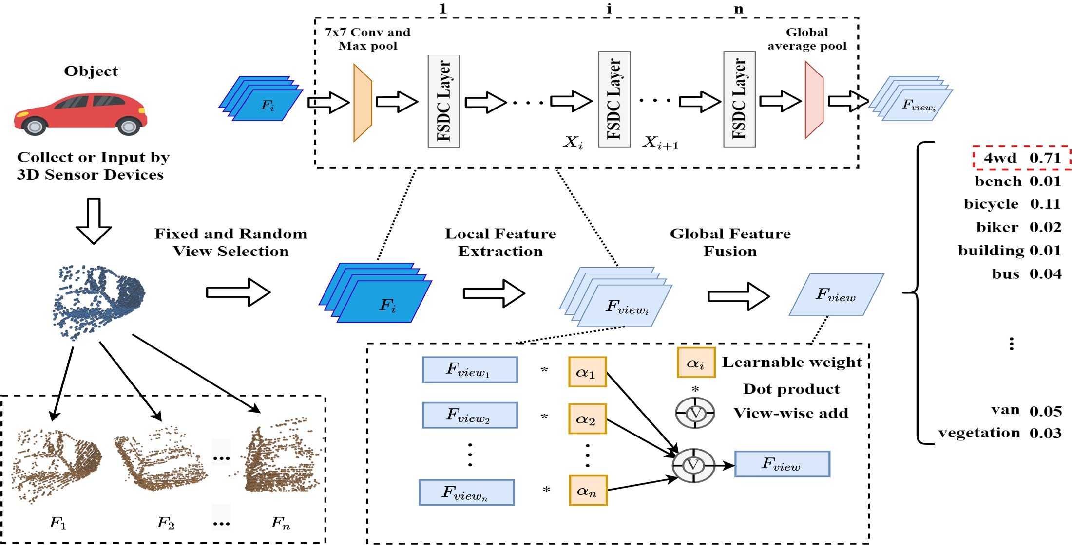
Normalization of point cloud spatial location: Because the location distribution of the original point cloud group may be inconsistent, the virtual camera must move the viewpoint to the center of different objects. Therefore, we normalize the position information of each point of all the point clouds to build its position distribution around the origin of the 3D coordinate system. Normalization is represented by Equation (1) as follows:

$$p_{i,j,k}=\frac{p_{i,j,k}-min(P_{X,Y,Z})}{max(P_{X,Y,Z})-min(P_{X,Y,Z})}$$

(1)

where $p_{i,j,k}$ is any point in the point cloud, and $min(P_{X,Y,Z})$ and $max(P_{X,Y,Z})$ represent the points obtained by taking the minimum and maximum values, respectively, of the X, Y, and Z coordinate axes in the point cloud.

(2)

Fixed viewpoint generation: Next, viewpoint selection is required. Since it is more complex to fix the original point cloud and then move the virtual camera frequently in space, we use an equivalent method, which is to rotate the object around a stationary virtual camera. We define a set of rotation angles, $\Theta =\left\{\right({\theta }_x,{\theta }_y,{\theta }_z\left)\right|{\theta }_x,{\theta }_y,{\theta }_z\in [0,{360}^{\circ }\left)\right\}$, where ${\theta }_x,{\theta }_y,{\theta }_z$ represent the rotation angles of the original point cloud in $X$, $Y$, and $Z$ coordinates, respectively. We rotate the object at equal intervals on the remaining coordinate axis, use the virtual camera for 2D projection, and choose the required view on the fixed viewpoint. Then, we place the virtual camera in a fixed position, keep the positions of two coordinate axes unchanged, rotate at equal intervals on the third coordinate axis, employ the virtual camera for 2D projection, and select the required view on the fixed viewpoint.

(3)

Random viewpoint generation: Then, we randomly generate $({\theta }_x,{\theta }_y,{\theta }_z)$ on the rotation angle set of the original point cloud and rotate the center point of the object to this angle. The virtual camera is used for projection to obtain the required view on the random viewpoint.

(4)

Multiview selection of fixed and random views: After many views are selected from fixed and random viewpoints, they must be combined in a certain proportion to generate the ultimate multiview representation in the initial stage. It is assumed that the fixed view set $fixed(\Theta )$ and the random view set $rand(\Theta )$ have been obtained by the fixed and random projection methods, respectively. $n$ represents the number of views and $t$ is the number of random views. Defining $F_i$ as the i-th view, $P$ indicates the final multiview combination, as shown in Equation (2):

$$P=(F_1,F_2,\dots ,F_i,\dots ,F_n)={\displaystyle \sum _{i=1}^{n-t}fixed(\Theta )}+{\displaystyle \sum _{j=1}^{t}rand(\Theta )}$$

(2)

In practice, when $n<6$, we take the view obtained from the fixed viewpoint; thus, $t=0$. Otherwise, we add one random view for every five fixed views, i.e., $t=\lfloor \frac{s}{6}\rfloor$. The original multiview combination in different conditions is represented by Equation (3) as follows:

$$P=(F_1,F_2,\dots ,F_i,\dots ,F_n)=\{\begin{array}{cc}{\displaystyle \sum _{i=1}^{s}fixed(\Theta )}& if n<6\\ {\displaystyle \sum _{i=1}^{n-t}fixed(\Theta )+{\displaystyle \sum _{j=1}^{t}rand(\Theta ), t=\lfloor \frac{s}{6}\rfloor }}& if n \ge 6\end{array}$$

(3)

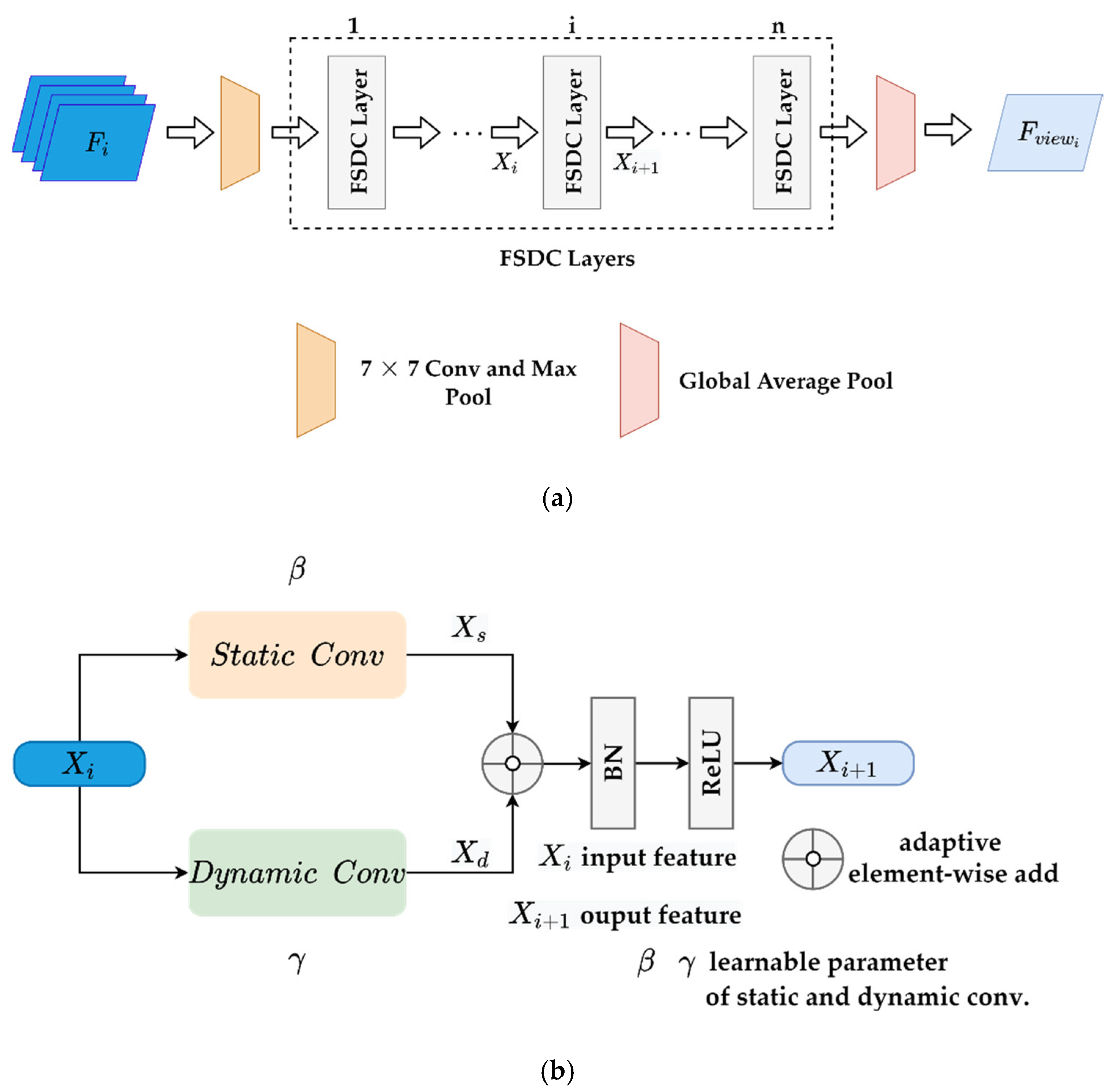
2.2. FSDC Local Feature Processing Operator

FSDC local feature extraction is shown in Figure 4, which has two subfigures. Figure 4a involves the conversion of the i-th view in the multiview representation $P$ of the 3D point cloud obtained by the fixed and random viewport selection into the local view representation $F_{vie{w}_i}$. After $7\times 7$ convolution and maximum pooling, it serially passes through n FSDC layers to obtain $F_{vie{w}_i}$ through global average pooling. The details of the i-th FSDC layer in Figure 3a are shown in Figure 4b. The layer extracts fine-grained features by applying static convolution ($3\times 3$ convolution of a ResNet50, ResNext50, and SENet50 network) and our proposed lightweight dynamic convolution generation operator to the input feature $X_i$ in parallel, adaptively fuses the features of the two branches via weight parameters $\beta$ and $\gamma$, and thereby obtains the output feature $X_{i+1}$ through the BN and ReLU layers.

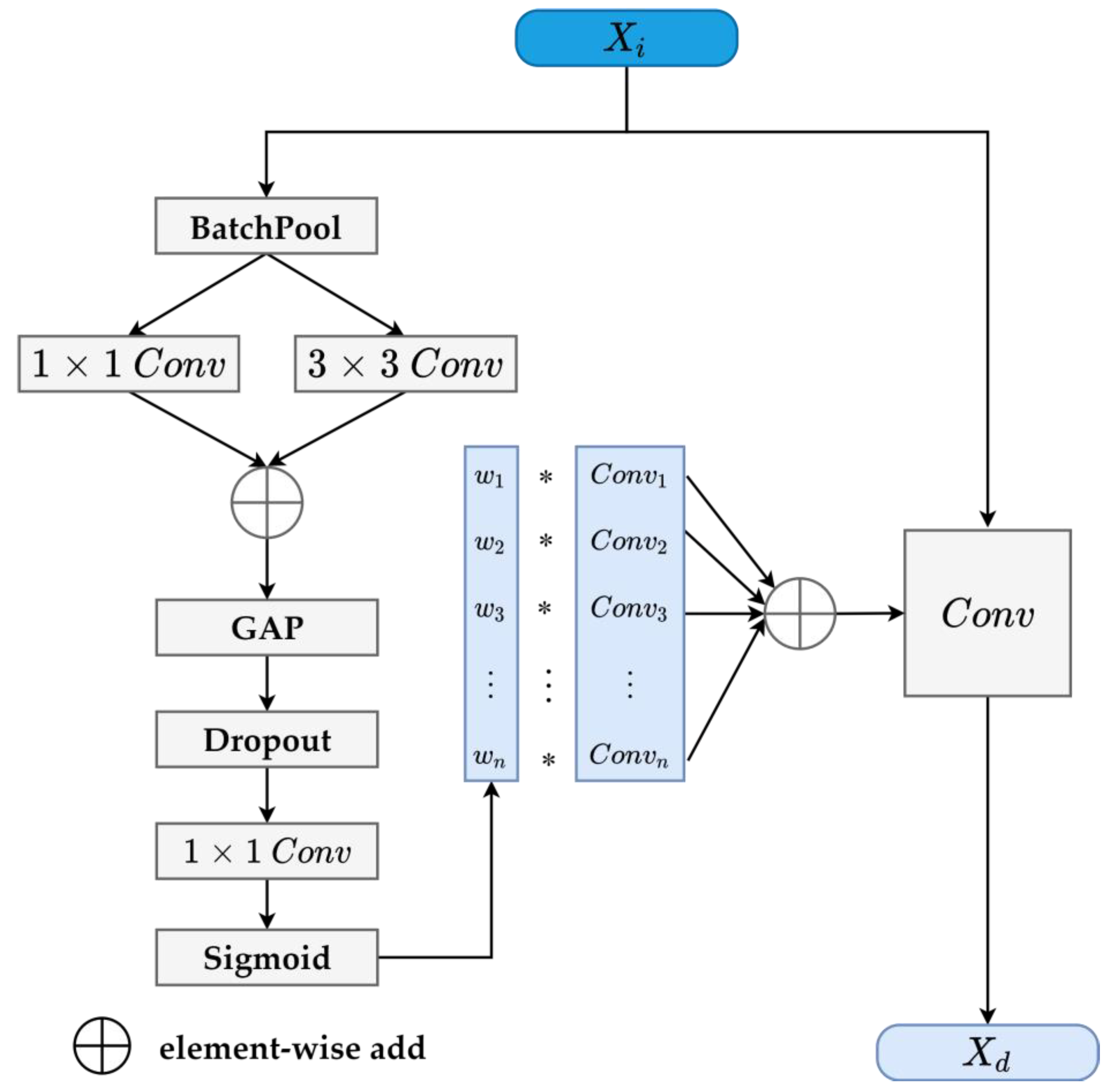
2.2.1. Lightweight Dynamic Convolution Generator

A series of convolution and pooling operations in the CNN extract features from images. The convolution kernel is weight-shared and suitable for processing high-dimensional data; however, there are drawbacks, e.g., the parameters of the whole network will be stationary after training, the adaptability is poor, and the flexibility is insufficient. Dynamic convolution [41,42] can avoid the problems of static convolution, but it is computationally complex and has a high memory overhead. Hence, we propose a more lightweight dynamic convolution operator, as shown in Figure 5. It has 6 steps.

① Architecture

(1)

Pooling of batch size dimension: First, we define a batch pool function, which fuses the original input feature map $X_i$ in the batch dimension to achieve a lightweight effect and ensure that the most critical feature information is obtained; the function is defined in Equation (4) as follows:

$$Z_1=BatchPool(X_i)=\frac{1}{b}{\displaystyle \sum _{j=1}^b{X}_i(j,c,h,w)}$$

(4)

where $X_i,Z_1$ indicate the input and output features of $BatchPool$, respectively; $X_i(j,c,h,w)$ represents an input image; $b$ is the number of batch sizes; and $c$, $h$, and $w$ are the channel, height, and width of the input features, respectively. The dimensions of the original $X_i$ are $b\times c\times h\times w$ and the dimensions of $Z_1$ as processed by the batch pool function are $1\times c\times h\times w$.

(2)

Convolution operation on different receptive fields: The original input features are convoluted from different receptive fields using 1 × 1 and 3 × 3 convolution, shown in Equations (5) and (6) as follows:

$$Z_2=W_1(Z_1)$$

(5)

$$Z_3=W_2(Z_1)$$

(6)

where $W_1$ and $W_2$ are the $1\times 1$ and $3\times 3$ convolution matrices, respectively, and $Z_2$ and $Z_3$ are the corresponding output features. The receptive field of the $1\times 1$ convolution is relatively small and is used to integrate the information of each pixel in the spatial dimension, while the receptive field of the 3 × 3 convolution is relatively large and can obtain more neighborhood information around pixels.

(3)

Fusion of information from different receptive fields: We add the output features $Z_2$ and $Z_3$ element by element and shrink them to $Z_4$, whose dimensions are $1\times c\times 1\times 1$, using spatial average pooling, as shown in Equation (7):

$$Z_4=\frac{1}{h\times w}{\displaystyle \sum _{i=1}^h{\displaystyle \sum _{j=1}^w(Z_2}}(1,c,i,j)+Z_3(1,c,i,j))$$

(7)

(4)

Dropout to avoiding overfitting: The dropout layer causes the neurons to randomly inactivate in a certain proportion, which can avoid overfitting while dynamically generating convolution, as shown in Equation (8) below:

$$Z_5=f_{dropout}(Z_4,p)$$

(8)

where p is the proportion of inactivation and $0<p<1$.

(5)

Generation of dynamic weight: Here, we change the original dynamic weight to the appropriate number of channels through the $1\times 1$ convolution of W₃ and employ sigmoid activation to obtain a probability between 0 and 1 as the dynamic weight to generate the final convolution layer, as shown in Equation (9) below:

$$\Omega =({\omega }_1,\dots ,{\omega }_i,\dots ,{\omega }_n,)={\sigma }_{sigmoid}{W}_3(Z_5)$$

(9)

where $\Omega =({\omega }_1,{\omega }_2,\cdots ,{\omega }_n)$ is a $1\times n$ vector of the generated dynamic convolution weights.

(6)

Generation of dynamic convolution kernel: Next, we multiply the original $n$ groups of convolution kernels $K$ by the dynamically generated weights $\Omega$ to generate the final dynamic convolution kernels, as shown in Equation (10):

$$Con{v}_{dynamic}=\Omega \times K={\displaystyle \sum _{i=1}^n{\omega }_{i}Con{v}_i}$$

(10)

② Performance Analysis

(1)

Parameters

It is assumed that the number of convolution input and output channels is $c_{in}$ and $c_{out}$, respectively, which are equal to $c$. The size of the output feature map is $n=h_{out}\times w_{out}$, where $h_{out}$ and $w_{out}$ are the height and width, respectively, of the output feature map. The convolution kernels are represented by $k\times k$, and the batch size by $b$. FSDC dynamic convolution employs the pooling of the batch size dimension, which reduces the parameter $b{c}^2{k}^2$ of the original dynamic convolution to $c^2{k}^2$, while the parameter of the traditional static convolution is also $c^2{k}^2$; hence, the final parameter is $2c^2{k}^2$.

(2)

FLOPs

As is shown in Equation (11), the floating-point operations (FLOPs) of traditional static convolution are about $2n{c}^2{k}^2$, i.e.,

$$\begin{array}{l}{c}_{out}(c_{in}\times k\times k+c_{in}(k\times k-1)+c_{in}-1)\times h_{out}\times w_{out}\\ =c_{out}(k^2{c}_{in}+k^2{c}_{in}-1)\times h_{out}\times w_{out}\\ =(2k^2{c}_{in}-1)c_{out}{h}_{out}{w}_{out}\\ =(2k^{2}c-1)cn\\ \approx 2n{c}^2{k}^2\end{array}$$

(11)

and the main FLOPs of FSDC dynamic convolution are reflected when the final generated dynamic convolution kernel participates in convolution. Consequently, we can refer to traditional static convolution, whose FLOPs are approximately $2n{c}^2{k}^2$; thus, the total computation is $4n{c}^2{k}^2$.

Table 1. Comparison of static convolution, dynamic convolution, and FSDC in terms of parameters and computation.

Conv. Type	Static Conv.	Dynamic Conv.	FSDC
Parameters	$c^2{k}^2$	$b{c}^2{k}^2$	$2c^2{k}^2$
FLOPs	$2n{c}^2{k}^2$	$bn{c}^2{k}^2$	$4n{c}^2{k}^2$

shows that the general dynamic convolution computation is $bn{c}^2{k}^2$. The numbers of parameters and computations of FSDC convolution are only twice those of traditional static convolution; however, they are generally far less than those for the previous method of dynamic convolution, because a larger $b$ means a higher computational cost of dynamic convolution. It has been shown [43,44] that to obtain better performance, $b$ should often be large, i.e., $b>>4$. Hence, our method can combine the advantages of traditional static convolution and dynamic convolution, with a greatly reduced number of parameters and computations.

2.2.2. Adaptive Process Combining Static and Dynamic Convolution

Next, we combine static and dynamic convolution to make the most of their advantages. Specifically, two convolution branches are applied to the input feature $X_i$ to obtain the output features $X_s$ and $X_d$, which represent the output characteristics obtained by static and dynamic convolution, respectively. The learnable parameters $\beta$ and $\gamma$ are introduced as the corresponding weights of $X_s$ and $X_d$, respectively, and the final value can be written as shown in Equation (12):

$$X_{i+1}=\beta \times X_s+\gamma \times X_d$$

(12)

If $\beta =1$ and $\gamma =0$, the output feature $X_{i+1}$ will degenerate to $X_s$ as extracted by traditional static convolution; if $\beta =0$ and $\gamma =1$, it will be transformed to $X_d$ as extracted by the proposed lightweight dynamic convolution. Thus, different weights can be obtained through the continuous optimization of $\beta$ and $\gamma$ according to the input data, i.e., the features learned by static and dynamic convolution can be emphasized to more or less achieve the desired feature extraction effect.

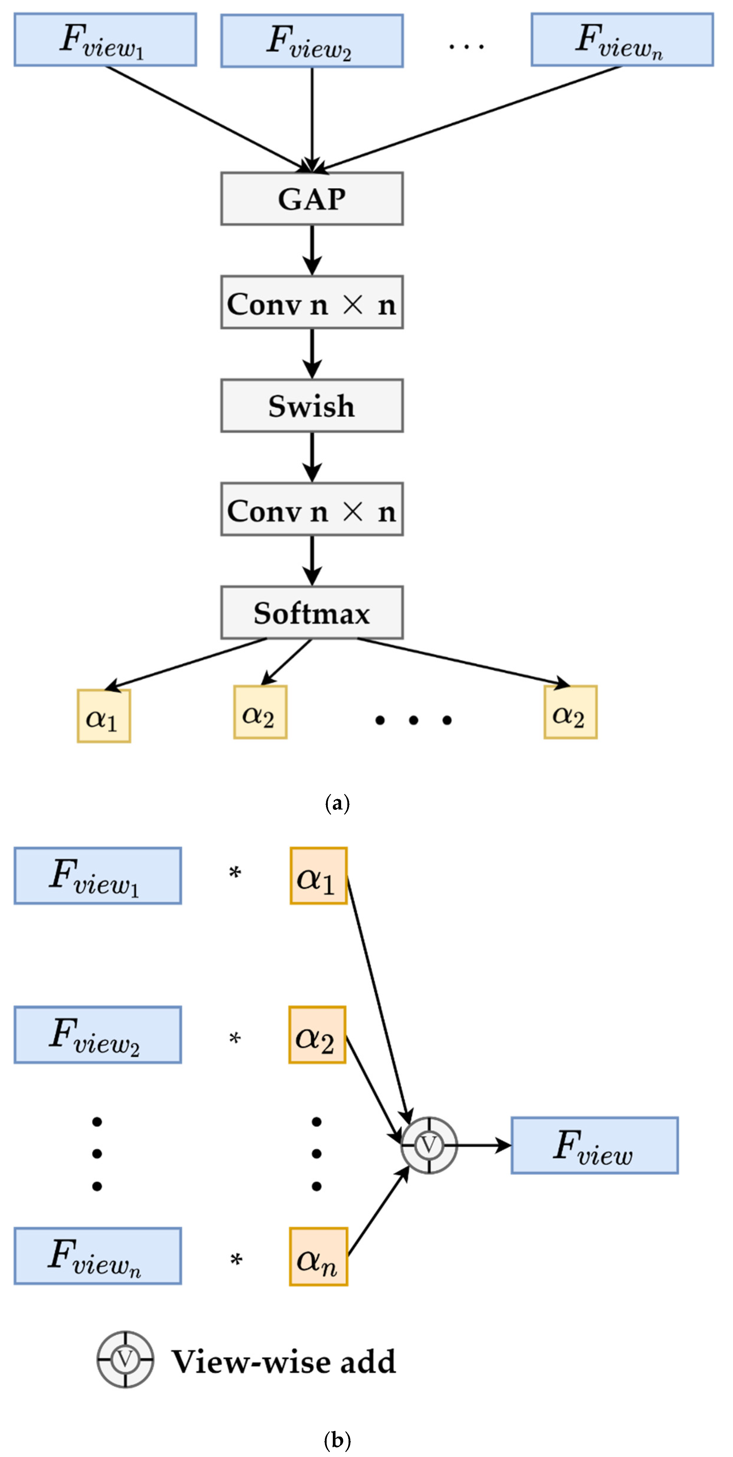
2.3. Adaptive Global Attention Pooling

An adaptive global attention pooling architecture, see Figure 6, is designed to fuse multiple local view features into an ultimate global view representation according to their importance for classification tasks. Figure 6a shows that different local views feature $F_{vie{w}_i}$ are operated by pooling, convolution, and Swish [45] activation functions, so as to learn their corresponding weight ${\alpha }_i$. Figure 6b shows that each local view feature $F_{vie{w}_i}$ is fused view-wise with the learned weight ${\alpha }_i$ to obtain the global view representation $F_{view}$. The proposed method considers the influence of different views to make the global representation more typical and representative in three steps.

(1)

Global average pooling (GAP) of local features: Global average pooling is applied to $n$ local features $F_{vie{w}_1},F_{vie{w}_2},\dots ,F_{vie{w}_n}$, and an n-dimensional vector is obtained as the initial value set of all dynamic weights, as shown in Equation (13) below:

$$A_1=\frac{1}{h\times w}{\displaystyle \sum _{i=1,j=1}^{h\times w}{f}_{i,j}}$$

(13)

where $A_1\in R^n$, and $h$ and $w$ are the height and width, respectively, of the local features. In general, either $H$ or $W$ is 1, and $f_{i,j}$ is the value of a feature at the subscript position.

(2)

Dynamic weight generation of local features: Next, we apply two $1\times 1$ convolutions to the n-dimensional vector and add a nonlinear activation function, Swish [45], between them. This is similar to the attention mechanism of SENet [46]; however, we do not squeeze and excite the channel, and the activation function is Swish. Then, the feature weight of each view can be acquired through the softmax activation function. The generation process is shown in Figure 5a. The dynamically generated weight is shown in Equation (14) below:

$$A_2={\sigma }_{soft\max }(Con{v}_{1\times 1}({\sigma }_{swish}(Con{v}_{1\times 1}(A_1))))$$

(14)

where ${\sigma }_{soft\max }$ and ${\sigma }_{swish}$ are the softmax and Swish activation functions, respectively, and Conv_1×1 is a $1\times 1$ convolution with $n$ input and output channels.

(3)

Global feature fusion: Finally, we multiply each view by its learned weight and add them in the view dimension. The ultimate global representation contains the feature information of all local views. The global representation fusion process is shown in Figure 5b and Equation (15):

$$F={\alpha }_1\times F_{vie{w}_1}+\dots +{\alpha }_i\times F_{vie{w}_i}+\dots +{\alpha }_n\times F_{vie{w}_n}$$

(15)

It should be noted that ${\alpha }_1,\dots ,{\alpha }_i,\dots ,{\alpha }_n$ are the components of weight $A_2$, and $F$ and $F_{vie{w}_i}$ are the final global representation and the i-th local feature, respectively.

3. Experiment

3.1. Dataset

We used the ModelNet40 [47] and Sydney Urban Objects [48] datasets for training and testing in our experiment. ModelNet40 is a dense point cloud dataset, completely synthesized by a computer, which simulates point cloud data under idealized conditions. It was chosen to reflect the accuracy of our proposed algorithm in point cloud classification due to its noise-free data. Sydney Urban Objects is a sparse point cloud dataset obtained via LiDAR scanning of outdoor scene objects in Sydney, Australia. The datasets contain a considerable amount of noise, local deformity, and uneven point density, which could be used to test the robustness and accuracy of FSDCNet in a real sparse point cloud classification task.

ModelNet40 is a widely used dataset for multiview 3D point cloud classification. It was published by Princeton University and contains 662 object categories and 127,915 CAD models. ModelNet40 selects 40 categories of objects, including aircraft, bathtub, bed, and bench, with a total of 12,314 CAD models. It contains 26 object categories, including common urban road objects, such as vehicles, pedestrians, buildings, and trees, with a total of 631 point clouds. Figure 7 and Figure 8 show several models from the two datasets.

3.2. Implementation

The hardware used for all experiments included a Nvidia Titan XP dual graphics card, 64 GB random access memory (RAM), and a 256 GB solid-state disk. The operating system used was Ubuntu 20.04, and the software included Blender 2.92.0 to preprocess the point cloud, PyTorch 1.7.1, and compute unified device architecture (CUDA) 10.1. The initial learning rate was set to 0.0001. An Adam optimizer was used for the gradient update. Several strategies were used to prevent model overfitting, including L2 regularization and a weight decay coefficient of 0.0001. The batch size was set to 128 for a single view, 16 for 6 views, and eight for 12 views. We constructed a point cloud dataset corresponding to the original ModelNet40 dataset by sampling 9999 points for each mesh. No preprocessing was required for the Sydney Urban Objects dataset, which was in scanned point cloud format. All multiviews were generated from the original point clouds of the two datasets according to the fixed and random perspective method. For ModelNet40, 108,732 views and 29,616 views were generated in the training set and testing set, respectively; for Sydney Urban Objects, 6954 views and 3156 views were generated in the training set and testing set, respectively. The training and testing periods were all set to 30 epochs.

3.3. Metrics

For the ModelNet40 dataset, the performance of the algorithm was evaluated by the overall accuracy (OA) and average accuracy (AA). In the training set, $\Delta$ is the total number of samples, ${\Delta }_{true}$ is the number of samples correctly classified by FSDCNet, ${\delta }_i$ is the number of samples in class i, ${\delta }_{i(true)}$ is the number of samples correctly classified by FSDCNet in ${\delta }_i$, $c_i$ is the accuracy of the i-th class, and $n$ is the total number of classes. OA and AA were calculated according to Equations (16) and (17) as follows [9]:

$$OA=\frac{{\Delta }_{true}}{\Delta }$$

(16)

$$AA=\frac{c_1+c_2+\dots +c_n}{n},c_i=\frac{{\delta }_{i(true)}}{{\delta }_i}$$

(17)

The number of objects in each class of the Sydney Urban Objects dataset varies greatly. For instance, there are 88 car samples, and just one scooter sample. The correct judgment of a small sample class involves less computational cost and inference time than a large sample class; however, the influence of their weight on the final AA is indeed the same, which is clearly unjustified. This is because AA will be affected by a small sample class, resulting in sharp fluctuations. Replacing AA with the F1 score can effectively reduce the impact of such problems on the final evaluation. Hence, the measurement criteria used for the Sydney Urban Objects dataset were the OA and F1, which was calculated according to Equation (18) as follows [49]:

$$F1=\frac{2\times P\times R}{P+R}$$

(18)

where $P$ and $R$ are the average precision and recall, respectively, of all classes.

3.4. Experimental Results and Analysis

3.4.1. Comparison with State-of-the-Art Methods

We compared FSDCNet with the most advanced point cloud classification models, including VoxelNet, VRN, Orion, and LightNet, which are voxel-based; PointNet, PointNet++, PointGrid, PointASNL, SimpleView, and ECC, which are based on a direct point cloud; and MVCNN, GVCNN, MVTN, and MHBN, which are view-based. It can be seen from Table 2a that on the ModelNet40 dataset, the OA and AA of FSDCNet in 6 views were 94.6% and 93.3%, respectively, compared to 94.1% and 92.2%, respectively, for the best comparison method, MHBN. For 12 views, the OA and AA of FSDCNet reached 95.3% and 93.6%, respectively, which were the highest values among all the models. From Table 2b, on the Sydney Urban Objects dataset, FSDCNet had an OA of 85.3% and an F1 score of 83.6% on 6 views. LightNet had the best classification accuracy among the point cloud-based models, and its F1 score was 79.8%. In 12 views, the OA of FSDCNet was 85.5% and the F1 score was 83.7%. Compared with other point cloud classification algorithm models, the evaluation metrics in the Sydney Urban Objects dataset were also superior. We also obtained the OA and F1 metrics for 6 views of MVCNN and GVCNN on the Sydney Urban Objects dataset. It can be seen that the two indicators of our FSDCNet in a single view were approximately equivalent to the 6 views of MVCNN. FSDCNet in 6 views was also much better than GVCNN’s, where the OA and F1 metrics of our model were 1.4% and 1.1% higher than those of the counterpart, respectively. This demonstrates that FSDCNet has broad applicability and can achieve state-of-the-art classification effects on both dense and sparse point clouds. On the one hand, the multiple views selected by the traditional fixed viewpoint are not conducive to the generalization of the model, i.e., accuracy will be greatly reduced in a viewpoint that has not been seen, or there will be large differences between the training set and the test set. In contrast, our model applies fixed and random viewpoint selection, which can increase its generalization performance, i.e., it can improve the accuracy of the classification of unknown viewpoints and is flexible. On the other hand, with the fusion of dynamic and static convolution, as found in our local feature extraction operator, we can combine their advantages in an adaptive approach to achieve a better feature extraction effect. Most models adopt traditional static convolution; thus, abundant and fine-grained information cannot be extracted. In addition, the proposed model assigns different weights to views according to their importance through adaptive global attention pooling, such that the final fusion-generated global view is more representative. Other point cloud pooling methods, e.g., average pooling and maximum pooling, cannot achieve this level of performance.

Table 2. Performance comparison of classification algorithms based on the ModelNet40 and Sydney Urban Objects datasets.

(a) ModelNet40
Method	Views	Modality	OA	AA
VoxelNet [50]	-	Voxel	-	83.0
VRN [51]	-	Voxel	-	91.3
3D Capsule [52]	-	Point	89.3	-
PointNet [10]	-	Point	89.2	86.2
PointNet++ [11]	-	Point	91.9	-
PointGrid [53]	-	Point	92.0	88.9
PointASNL [31]	-	Point	93.2	-
SimpleView [54]	-	Point	93.9	91.8
MVCNN [9]	12	Views	92.1	89.9
GVCNN [12]	12	Views	92.6	-
MVTN [55]	12	Views	93.8	92.0
MHBN [13]	6	Views	94.1	92.2
FSDCNet (ours)	1	Views	93.8	91.2
FSDCNet (ours)	6	Views	94.6	93.3
FSDCNet (ours)	12	Views	95.3	93.6
(b) Sydney Urban Objects
Method	Views	Modality	OA	F1
VoxelNet [50]	-	Voxel	-	73.0
ORION [56]	--	Voxel	-	77.8
ECC [57]	-	Point	-	78.4
LightNet [58]	-	Voxel	-	79.8
MVCNN [9]	6	Views	81.4	80.2
GVCNN [12]	6	Views	83.9	82.5
FSDCNet (ours)	1	Views	81.2	80.1
FSDCNet (ours)	6	Views	85.3	83.6
FSDCNet (ours)	12	Views	85.5	83.7

Table 2. Performance comparison of classification algorithms based on the ModelNet40 and Sydney Urban Objects datasets.

(a) ModelNet40
Method	Views	Modality	OA	AA
VoxelNet [50]	-	Voxel	-	83.0
VRN [51]	-	Voxel	-	91.3
3D Capsule [52]	-	Point	89.3	-
PointNet [10]	-	Point	89.2	86.2
PointNet++ [11]	-	Point	91.9	-
PointGrid [53]	-	Point	92.0	88.9
PointASNL [31]	-	Point	93.2	-
SimpleView [54]	-	Point	93.9	91.8
MVCNN [9]	12	Views	92.1	89.9
GVCNN [12]	12	Views	92.6	-
MVTN [55]	12	Views	93.8	92.0
MHBN [13]	6	Views	94.1	92.2
FSDCNet (ours)	1	Views	93.8	91.2
FSDCNet (ours)	6	Views	94.6	93.3
FSDCNet (ours)	12	Views	95.3	93.6
(b) Sydney Urban Objects
Method	Views	Modality	OA	F1
VoxelNet [50]	-	Voxel	-	73.0
ORION [56]	--	Voxel	-	77.8
ECC [57]	-	Point	-	78.4
LightNet [58]	-	Voxel	-	79.8
MVCNN [9]	6	Views	81.4	80.2
GVCNN [12]	6	Views	83.9	82.5
FSDCNet (ours)	1	Views	81.2	80.1
FSDCNet (ours)	6	Views	85.3	83.6
FSDCNet (ours)	12	Views	85.5	83.7

3.4.2. Influence of the Multi-Perspective Selection Method

Fixed and random viewpoint selection methods were adopted. The AA metrics of the two methods were compared on 6 and 12 views. According to Formula 3, in the fixed and random viewpoint selection methods, 6 views consisted of five fixed views and one random view, and 12 views consisted of 10 fixed views and two random views. As can be seen from

Table 3. Comparison of the classification performance of different viewpoint selection methods.

(a) ModelNet40
Preprocessing	Views	OA
Fixed	6	94.1
Fixed and random	6	94.6
Fixed	12	94.7
Fixed and random	12	95.3
(b) Sydney Urban Objects
Preprocessing	Views	OA
Fixed	6	84.1
Fixed and random	6	85.3
Fixed	12	84.9
Fixed and random	12	85.5

, the AA metrics of the ModelNet40 and Sydney Urban Objects datasets in 6 and 12 views were improved by a certain proportion after the fixed and random viewpoint selection method. From Table 3a, for the ModelNet40 dataset, if fixed and random viewpoints were employed, the OA of 6 and 12 views reached 94.6% and 95.3%, respectively. In contrast, the OA of 6 and 12 views reached 94.1% and 94.7%, respectively, if only a fixed viewpoint was employed. From Table 3b, for the Sydney Urban Objects dataset, if fixed and random viewpoints were employed in 6 and 12 views, their OAs were 85.3% and 85.5%, respectively, while the OAs were 84.1% and 84.9%, respectively, if using only fixed viewpoints. Therefore, it can be concluded that for views selected from the traditional fixed viewpoint, combining some views obtained from the random viewpoint can increase the accuracy and even the robustness of model classification, such that the model can learn some features that cannot be learned from the fixed viewpoint. However, the number of views selected from random viewpoints cannot be too large, as the accuracy of the model will decline sharply. This is because the different views generated by these random viewpoints will have considerable differences, which will reduce the data correlation of the training and test sets or even cause them to be completely different, affecting the accuracy of classification.

3.4.3. Influence of the Number of Views

In the evaluation of the classification performance of FSDCNet on different views, we sought a tradeoff between classification performance and computational storage cost. In the experiment, the number of views was set to 1, 6, and 12, so as to compare the OA, AA, and F1 metrics of FSDCNet and other advanced multiview classification models using the ModelNet40 and Sydney Urban Objects datasets. From

Table 4. Influence of the number of views on classification performance.

(a) ModelNet40
Method	Views	OA	AA
MVCNN [9]	6	92.0	-
MVCNN [9]	12	91.5	-
GVCNN [12]	12	92.6	-
MVTN [55]	12	93.8	92.0
MHBN [13]	6	94.1	92.2
MHBN [13]	12	93.4	-
FSDCNet (ours)	1	93.8	91.2
FSDCNet (ours)	6	94.6	93.3
FSDCNet (ours)	12	95.3	93.6
(b) Sydney Urban Objects
Method	Views	OA	F1
VoxelNet [50]	-	-	73.0
ORION [56]	-	-	77.8
ECC [57]	-	-	78.4
LightNet [58]	-	-	79.8
MVCNN [9]	6	81.4	80.2
GVCNN [12]	6	83.9	82.5
FSDCNet	1	81.2	80.1
FSDCNet	6	85.3	83.6
FSDCNet	12	85.5	83.7

a, it can be seen that the OA and AA of FSDCNet in a single view were 93.8% and 91.2%, respectively, on ModelNet40, which were higher than those of MVCNN in 6 and 12 views and of GVCNN in 12 views. The OA and AA of FSDCNet in 6 views were 94.6% and 93.2%, respectively, and the corresponding metrics of MHBN were 94.1% and 92.2%, respectively. The OA and AA of FSDCNet reached 95.3% and 93.6%, respectively, in 12 views, which were much higher than those of the most advanced multiview classification models. From Table 4b, it can be seen that the OA and F1 score of FSDCNet on the Sydney Urban Objects dataset were 81.2% and 80.1%, respectively, in a single view; 85.3% and 83.6%, respectively, in 6 views; and 85.5% and 83.7%, respectively, in 12 views. The F1 score of LightNet, which showed excellent performance among these models (Table 4b), was only 79.8%, while that of FSDCNet was 0.3%, 3.8%, and 3.9% higher in 1, 6, and 12 views, respectively. It is worth noting that the classification performance of FSDCNet in a single view was better than that of most of the compared point cloud classification models on both the ModelNet40 and Sydney Urban Objects datasets.

Overall, with an increase in the number of views, the OA, AA, and F1 metrics of FSDCNet also increased. In contrast, the classification performance of MHBN in 12 views was poorer than that in 6 views, which shows that our algorithm is more robust than MHBN and our model is not prone to jitter. The ModelNet40 dataset showed significantly better performance than the Sydney Urban Objects dataset. We believe that this is because Sydney Urban Objects is a sparse point cloud dataset taken from the real world with a small number of samples; hence, it lacks sufficient learning data. In addition, since its data were scanned by LiDAR in a real scene, it contains a considerable amount of noise. Since the noise increases with the number of views, the model learns more noisy data, which will eventually affect its classification performance.

3.4.4. Influence of Static Convolution and Dynamic Convolution

In the local feature extraction module of FSDCNet, dynamic and static convolution work together to obtain the local feature information of the view, which is the basis of the subsequent global feature fusion. For the static convolution part, the convolution of any existing 2D CNN model can be applied. Here, we employed the three most commonly used models—ResNet50, ResNext50, and SENet50—and compared the OA, AA, and F1 metrics of the models with and without our proposed lightweight dynamic convolution. All comparisons were made in 6 views in order to balance storage overhead and accuracy improvement. As can be seen from Table 5, the classification accuracy of the two datasets improved after combining lightweight dynamic convolution and the proposed adaptive weight parameter fusion. The OA and AA of the ResNet50 network model on the ModelNet40 dataset were 93.0% and 92.0%, respectively. Combined with lightweight dynamic convolution, the OA and AA were 93.8% and 92.6%, respectively. On the Sydney Urban Objects dataset, the OA and F1 score of the original ResNet50 were 83.1% and 81.7%, respectively. Combined with lightweight dynamic convolution, they were 84.5% and 82.3%, respectively. Similarly, it can be seen in Table 5 that for ResNext50, the OA and AA on ModelNet40 increased by 1.2% and 0.5%, respectively, while the OA and the F1 score on Sydney Urban Objects increased by 1.0% and 0.8%, respectively. For SENet50, the OA and AA on ModelNet40 increased by 1.1% and 1.0%, respectively, and by 1.3% and 1.4%, respectively, on Sydney Urban Objects. Through the above comparisons, we can conclude that, after using static convolution and our proposed lightweight dynamic convolution branch in parallel, these metrics were enhanced to some degree.

Table 5. Comparison of classification performance between static and dynamic convolution.

CNN Model	ModelNet40		Sydney Urban Objects
	OA	AA	OA	F1
ResNet50 [59]	93.0	92.0	83.1	81.7
FSDCNet-ResNet50	93.8	92.6	84.5	82.3
ResNext50 [60]	92.9	92.2	83.8	81.7
FSDCNet-ResNext50	94.1	92.7	84.8	82.5
SENet50 [46]	93.5	92.3	84.0	82.2
FSDCNet-SENet50	94.6	93.3	85.3	83.6

Table 5. Comparison of classification performance between static and dynamic convolution.

CNN Model	ModelNet40		Sydney Urban Objects
	OA	AA	OA	F1
ResNet50 [59]	93.0	92.0	83.1	81.7
FSDCNet-ResNet50	93.8	92.6	84.5	82.3
ResNext50 [60]	92.9	92.2	83.8	81.7
FSDCNet-ResNext50	94.1	92.7	84.8	82.5
SENet50 [46]	93.5	92.3	84.0	82.2
FSDCNet-SENet50	94.6	93.3	85.3	83.6

When investigating the reason for this, we found that lightweight dynamic convolution can extract some fine-grained feature information that cannot be obtained by traditional static convolution, and this is more conducive to the final model classification. Moreover, lightweight dynamic convolution and static convolution are combined adaptively, which can better integrate the features of different dimensions.

3.4.5. Influence of Fusion Strategy

The fusion strategy of dynamic and static convolution is mainly completed through the learnable parameters $\beta$ and $\gamma$, as shown in Equation (12). If we analyze the fusion strategy in detail, it largely depends on the impact of using or not using the learnable parameters $\beta$ and $\gamma$ on the classification performance. It should be noted that when the learnable parameters $\beta$ and $\gamma$ are used, their initial values are set to 1.0, and the values of $\beta$ and $\gamma$ will be dynamically updated with the back propagation of the network. When the learnable parameters $\beta$ and $\gamma$ are not used, the feature information extracted from the dynamic and static convolution branches is directly added element by element. Here, we presented some experimental results of the OA, AA, and F1 metrics in 6 and 12 views on two datasets, as shown in

Table 6. Comparison of classification performance with or without the learnable parameters $\beta$ and $\gamma$.

(a) ModelNet40
Learnable Parameters	6 views		12 views
	OA	AA	OA	AA
With $\beta$ and $\gamma$	94.6	93.3	95.3	93.6
Without $\beta$ and $\gamma$	94.2	92.0	94.9	93.1
(b) Sydney Urban Objects
Learnable Parameters	6 views		12 views
	OA	F1	OA	F1
With $\beta$ and $\gamma$	85.3	83.6	85.5	83.7
Without $\beta$ and $\gamma$	84.5	82.5	84.9	82.9

. As can be seen from Table 6a, for ModelNet40, the OA and AA indicators in 6 and 12 views increased by 0.4%, 1.3%, 0.4%, and 0.5%, respectively, after using learnable parameters. Similarly, Table 6b shows that, for the Sydney Urban Objects dataset, the OA and F1 indicators in 6 and 12 views increased by 0.8%, 1.1%, 0.6%, and 0.8%, respectively, after using the learnable parameters. The performance on the ModelNet40 and Sydney Urban Objects datasets were improved after using the learnable parameters $\beta$ and $\gamma$; however, the latter was better than the former. This shows that extracting local feature information via adaptive fusion outperforms the element-wise addition of the extracted features directly.

3.4.6. Influence of Pooling

Considering the tradeoff between storage overhead and accuracy improvement, we still used 6 views for evaluation. The most commonly used pooling methods, including maximum pooling, average pooling, maximum and average pooling, and soft pooling, were compared with the adaptive attention pooling method of FSDCNet. As shown in Table 7, the OA and AA of FSDCNet on the ModelNet40 dataset were 94.6% and 93.3%, respectively, compared to 94.2% and 92.5%, respectively, for maximum pooling. The OA and F1 score of FSDCNet were 85.3% and 83.6%, respectively, on the Sydney Urban Objects dataset, compared to 84.9% and 83.1%, respectively, for maximum pooling. These experiments demonstrate that our adaptive global attention pooling achieves the most desirable performance. It can learn a weight for each local view feature according to its importance and integrate different view features with learned weights into the final global view representation, so as to strengthen important features, weaken non-essential features, and integrate the most crucial information in multiple local views, contributing to the final classification and judgment of the 3D point cloud.

Table 7. Comparison of classification performance with different global pooling.

Method	ModelNet40		Sydney Urban Object
	OA	AA	OA	F1
MaxPooling	94.2	92.5	84.9	83.1
MeanPooling	93.7	92.1	84.1	82.3
Max+Mean	94.2	92.8	85.2	83.1
SoftPool [61]	93.7	91.9	84.5	83.0
FSDCNet (ours)	94.6	93.3	85.3	83.6

Table 7. Comparison of classification performance with different global pooling.

Method	ModelNet40		Sydney Urban Object
	OA	AA	OA	F1
MaxPooling	94.2	92.5	84.9	83.1
MeanPooling	93.7	92.1	84.1	82.3
Max+Mean	94.2	92.8	85.2	83.1
SoftPool [61]	93.7	91.9	84.5	83.0
FSDCNet (ours)	94.6	93.3	85.3	83.6

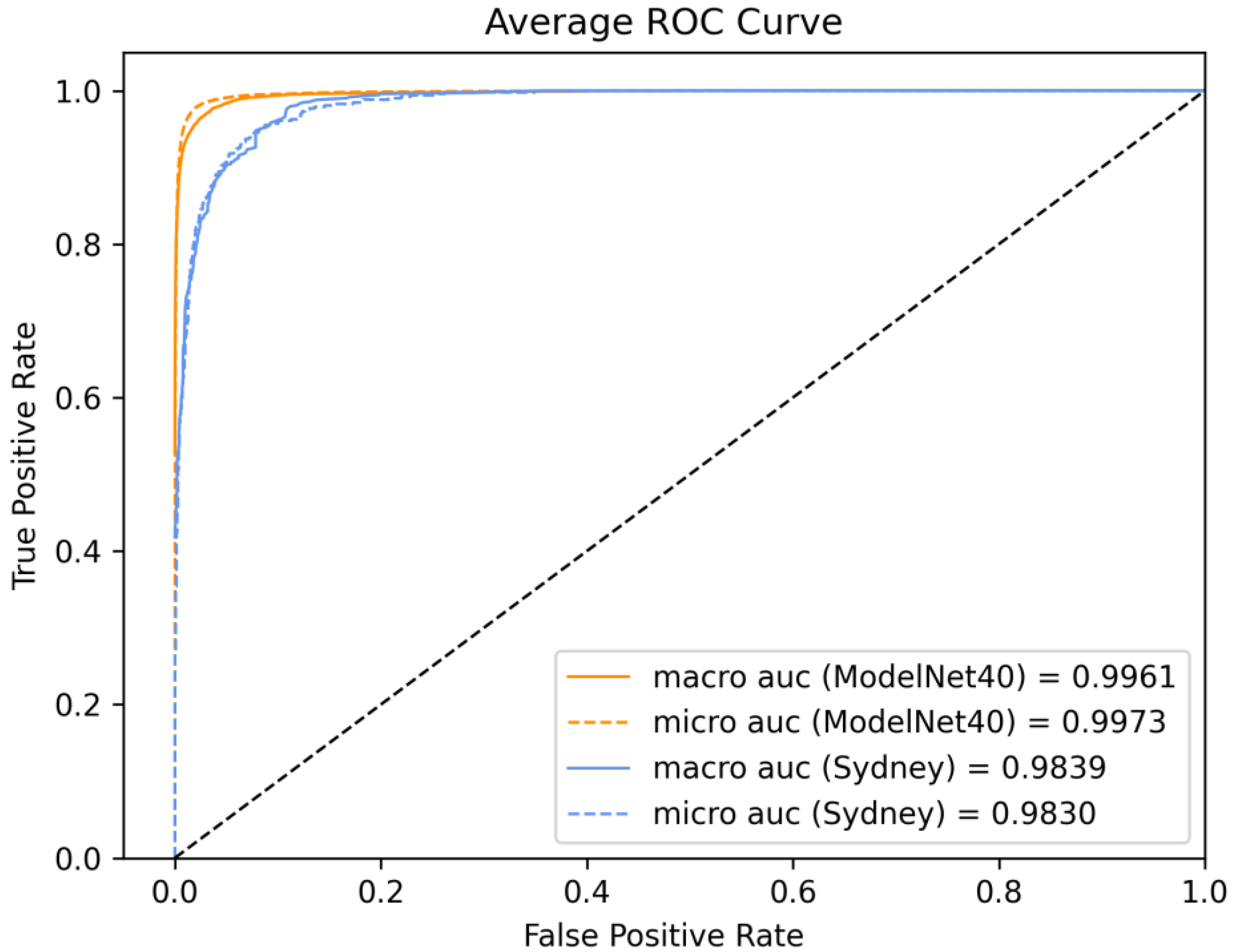
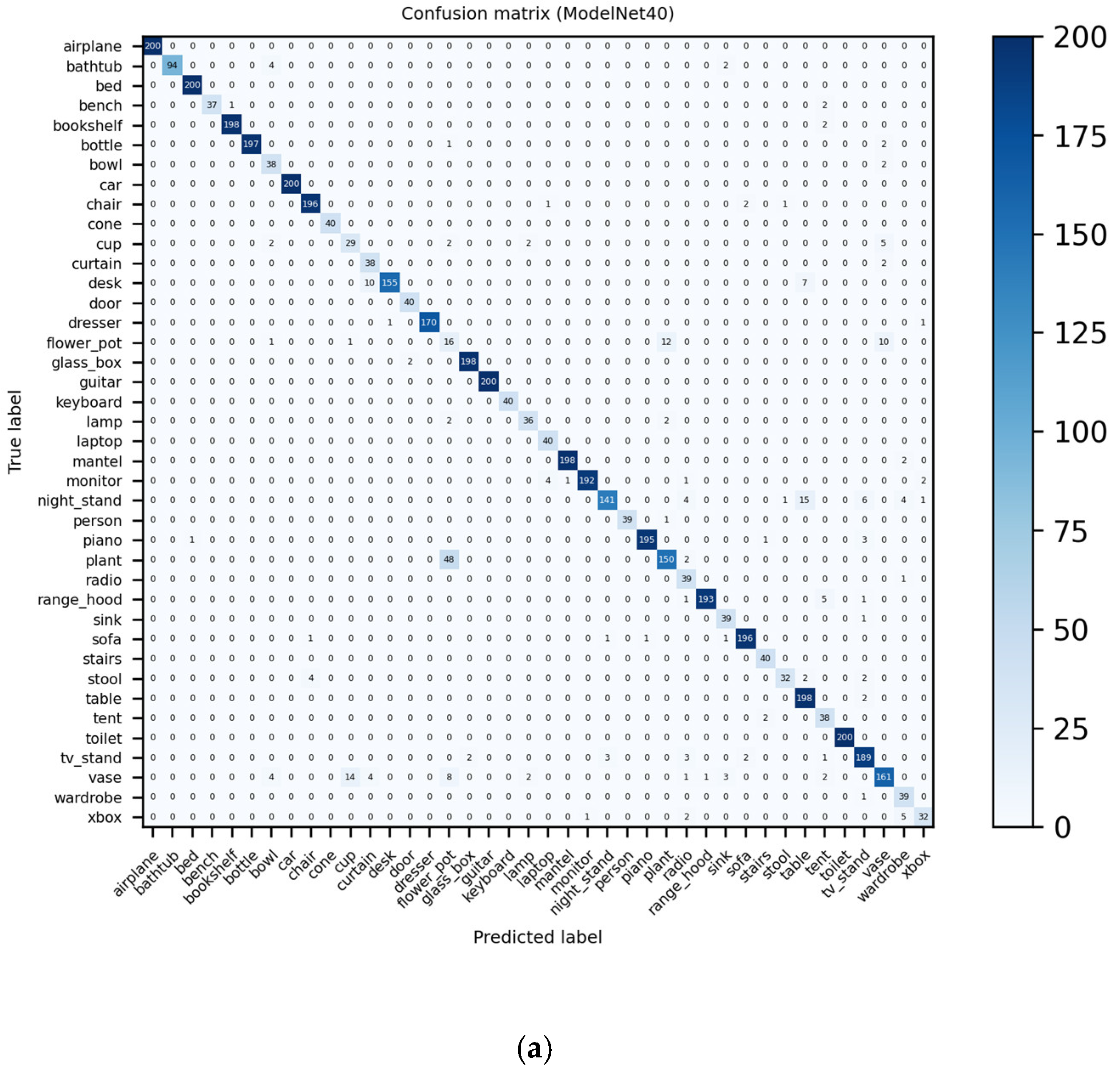
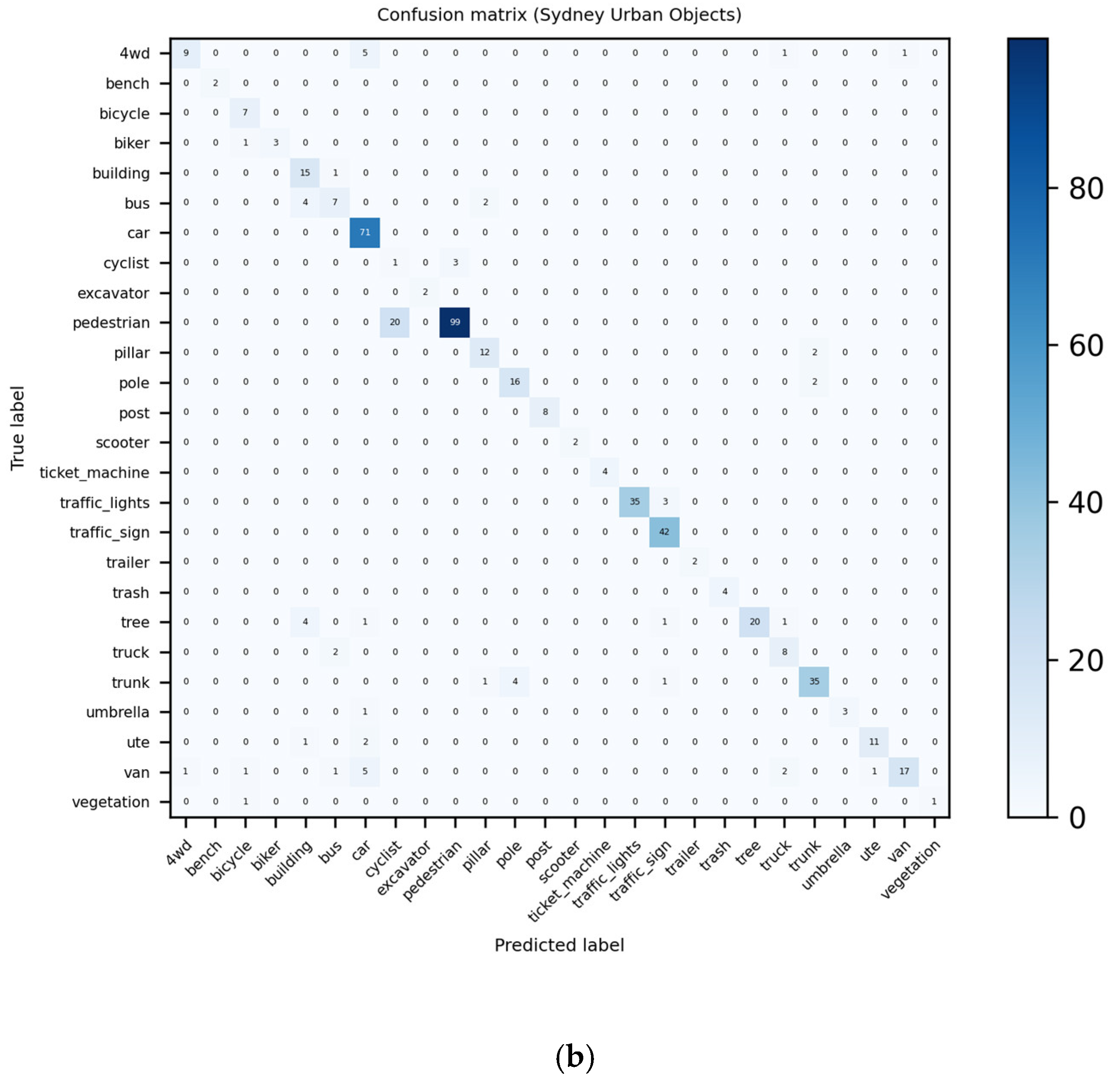
3.4.7. Visualization and Analysis of Confusion Matrices and ROC Curves

① Confusion matrices

A confusion matrix is usually used to more intuitively exhibit the classification performance of a model in various categories. It can clearly reveal which categories are easy to distinguish and which are difficult to determine. Figure 9 shows the confusion matrices of our FSDCNet on two datasets. Here, the most representative 6 views were selected to evaluate the classification performance of our model on each class. As can be seen from Figure 9a, for the ModelNet40 dataset, the classification accuracy of FSDCNet on some classes, e.g., aircraft, bathtub, bed, car, and cone, reached 100%. There were a few incorrect judgments about the classification of other classes, e.g., bench, bowl, and curtain. It is worth noting that FSDCNet had a high proportion of errors when judging plant objects. Among the 198 plant samples, 48 samples were misjudged as a flowerpot, accounting for about 24.2% of the plant samples. When investigating the reason for this, we found that there were several similar instances in the two classes. A certain proportion of plant samples contained both flowers (plants class) and flowerpots, leading to incorrect classification by the model. In contrast, the majority of classes in the ModelNet40 dataset had a high classification accuracy. As can be seen from Figure 9b, for the Sydney Urban Objects dataset, our FSDCNet also achieved 100% classification accuracy on some classes, e.g., bench, bicycle, car, and excavator, although some of these classes merely had a small number of instances. There were a few misjudged samples in several classes, e.g., building, traffic lights, and traffic signs. However, it is worth nothing that FSDCNet demonstrated a high proportion of errors when discriminating “pedestrian” objects. Among the 119 “pedestrian” samples, 20 samples were incorrectly judged as “cyclist”, accounting for about 16.8% of the “pedestrian” samples. We believe that the model learned human characteristics from “cyclist” and “pedestrian”, causing misjudgment in the actual classification. Overall, our FSDCNet model achieved excellent classification performance through the visual confusion matrix on the two datasets. Meanwhile, our experiments also show that FSDCNet has widespread applicability, not only to dense point clouds (ModelNet40), but also to sparse point clouds (Sydney Urban Objects).

② ROC curves

An receiver operating characteristic (ROC) curve reveals the relationship between the false positive rate (FPR) and true positive rate (TPR) under different thresholds, intuitively reflecting the impact of any threshold on the generalization performance of the model. We visualized the average ROC curves of all classes of FSDCNet on the two datasets and calculated the corresponding area under curve (AUC), as shown in Figure 10. Overall, FSDCNet achieved outstanding performance on the ModelNet40 and Sydney Urban Objects datasets; however, the indicator of the former was better than that of the latter. For the ModelNet40 dataset, when FPR was 0, its TPR reached about 0.95. For the Sydney Urban Objects dataset, when FPR was close to 0.1, its TPR reached about 0.95. The average macro- and micro-AUC of all classes were 0.9961 and 0.9973, respectively, on the ModelNet40 dataset. Similarly, the average macro- and micro-AUC were 0.9839 and 0.9830, respectively on the Sydney Urban Objects dataset. There was a slight discrepancy between the results from the two datasets. We believe this was due to the differences between the ModelNet40 and the Sydney Urban Objects datasets themselves. On the one hand, ModelNet40, as the representative of a dense point cloud dataset, simulates point cloud classification in the ideal environment. On the other hand, Sydney Urban Objects, which represents a sparse point cloud dataset, characterizes noisy point cloud classification in the real world. Therefore, the generalization performance of the former is better than that of the latter for the same classifier. However, the overall generalization performance of both is very high. This again shows that our FSDCNet model can not only achieve very high accuracy, but also has wide applicability.

4. Conclusions

Here, we proposed FSDCNet, a multiview 3D point cloud classification method based on a dynamic and static convolution fusion neural network. With the aim of resolving the problem of overfitting in the preprocessing stage of the traditional fixed view selection method, our FSDC model applies fixed and random viewpoint selection to improve the generalization performance of the model on different views. An adaptive weight fusion operator of static and dynamic convolution is used for local feature extraction in order to extract more fine-grained feature information. In addition, adaptive global attention pooling can more effectively integrate local features on different views and obtain the most critical detail in the global representation of the point cloud. Compared with some advanced 3D point cloud classification models, FSDCNet achieved state-of-the-art classification as measured by the OA, AA, and F1 score. Experiments on the ModelNet40 and Sydney Urban Objects datasets demonstrated that FSDCNet is not only suitable for the classification of dense point cloud data but can also achieve the best results for sparse point clouds with noise and local block defects, which shows its wide applicability. However, FSDCNet, similar to other convolutional neural networks, still needs a large number of sample datasets to support training and testing. Hence, in future work, we intend to introduce one-shot, zero-shot, vision transformer, and other technologies, such that FSDCNet can also achieve superior performance on small sample datasets.

References

1. Zhang, J.X.; Lin, X.G. Advances in fusion of optical imagery and LiDAR point cloud applied to photogrammetry and remote sensing. Int. J. Image Data Fusion 2017, 8, 1–31. [Google Scholar] [CrossRef]
2. Wentz, E.A.; York, A.M.; Alberti, M.; Conrow, L.; Fischer, H.; Inostroza, L.; Jantz, C.; Pickett, S.T.A.; Seto, K.C.; Taubenbock, H. Six fundamental aspects for conceptualizing multidimensional urban form: A spatial mapping perspective. Landsc. Urban Plan. 2018, 179, 55–62. [Google Scholar] [CrossRef]
3. Yue, X.Y.; Wu, B.C.; Seshia, S.A.; Keutzer, K.; Sangiovanni-Vincentelli, A.L.; Assoc Comp, M. A LiDAR Point Cloud Generator: From a Virtual World to Autonomous Driving. In Proceedings of the 8th ACM International Conference on Multimedia Retrieval (ACM ICMR), Yokohama, Japan, 11–14 June 2018; pp. 458–464. [Google Scholar]
4. Chen, X.Z.; Ma, H.M.; Wan, J.; Li, B.; Xia, T. Multi-View 3D Object Detection Network for Autonomous Driving. In Proceedings of the 30th IEEE/CVF Conference on Computer Vision and Pattern Recognition (CVPR), Honolulu, HI, USA, 21–26 July 2017; pp. 6526–6534. [Google Scholar]
5. Braun, A.; Tuttas, S.; Borrmann, A.; Stilla, U. Improving progress monitoring by fusing point clouds, semantic data and computer vision. Autom. Constr. 2020, 116, 103210. [Google Scholar] [CrossRef]
6. Jaritz, M.; Gu, J.Y.; Su, H. Multi-view PointNet for 3D Scene Understanding. In Proceedings of the IEEE/CVF International Conference on Computer Vision (ICCV), Seoul, Korea, 27 October–2 November 2019; pp. 3995–4003. [Google Scholar]
7. Duan, H.; Wang, P.; Huang, Y.; Xu, G.; Wei, W.; Shen, X. Robotics Dexterous Grasping: The Methods Based on Point Cloud and Deep Learning. Front. Neurorobot. 2021, 15, 1–27. [Google Scholar] [CrossRef] [PubMed]
8. Yang, Y.; Fang, H.R.; Fang, Y.F.; Shi, S.J. Three-dimensional point cloud data subtle feature extraction algorithm for laser scanning measurement of large-scale irregular surface in reverse engineering. Measurement 2020, 151, 107220. [Google Scholar] [CrossRef]
9. Su, H.; Maji, S.; Kalogerakis, E.; Learned-Miller, E. Multi-view Convolutional Neural Networks for 3D Shape Recognition. In Proceedings of the IEEE International Conference on Computer Vision, Santiago, Chile, 11–18 December 2015; pp. 945–953. [Google Scholar]
10. Qi, C.R.; Su, H.; Mo, K.C.; Guibas, L.J. PointNet: Deep Learning on Point Sets for 3D Classification and Segmentation. In Proceedings of the 30th IEEE/CVF Conference on Computer Vision and Pattern Recognition (CVPR), Honolulu, HI, USA, 21–26 July 2017; pp. 77–85. [Google Scholar]
11. Qi, C.R.; Yi, L.; Su, H.; Guibas, L.J. PointNet plus plus: Deep Hierarchical Feature Learning on Point Sets in a Metric Space. In Proceedings of the 31st Annual Conference on Neural Information Processing Systems (NIPS), Long Beach, CA, USA, 4–9 December 2017; pp. 4–9. [Google Scholar]
12. Feng, Y.F.; Zhang, Z.Z.; Zhao, X.B.; Ji, R.R.; Gao, Y. GVCNN: Group-View Convolutional Neural Networks for 3D Shape Recognition. In Proceedings of the 31st IEEE/CVF Conference on Computer Vision and Pattern Recognition (CVPR), Salt Lake City, UT, USA, 18–23 June 2018; pp. 264–272. [Google Scholar]
13. Yu, T.; Meng, J.J.; Yuan, J.S. Multi-view Harmonized Bilinear Network for 3D Object Recognition. In Proceedings of the 31st IEEE/CVF Conference on Computer Vision and Pattern Recognition (CVPR), Salt Lake City, UT, USA, 18–23 June 2018; pp. 186–194. [Google Scholar]
14. Wei, X.; Yu, R.X.; Sun, J. View-GCN: View-based Graph Convolutional Network for 3D Shape Analysis. In Proceedings of the IEEE/CVF Conference on Computer Vision and Pattern Recognition (CVPR), Seattle, WA, USA, 14–19 June 2020; pp. 1847–1856. [Google Scholar]
15. Li, L.; Zhu, S.Y.; Fu, H.B.; Tan, P.; Tai, C.L. End-to-End Learning Local Multi-View Descriptors for 3D Point Clouds. In Proceedings of the IEEE/CVF Conference on Computer Vision and Pattern Recognition (CVPR), Seattle, WA, USA, 14–19 June 2020; pp. 1916–1925. [Google Scholar]
16. Xiong, B.A.; Jiang, W.Z.; Li, D.K.; Qi, M. Voxel Grid-Based Fast Registration of Terrestrial Point Cloud. Remote Sens. 2021, 13, 1905. [Google Scholar] [CrossRef]
17. Plaza, V.; Gomez-Ruiz, J.A.; Mandow, A.; Garcia-Cerezo, A.J. Multi-layer Perceptrons for Voxel-Based Classification of Point Clouds from Natural Environments. In Proceedings of the 13th International Work-Conference on Artificial Neural Networks (IWANN), Palma de Mallorca, Spain, 10–12 June 2015; pp. 250–261. [Google Scholar]
18. Liu, Z.J.; Tang, H.T.; Lin, Y.J.; Han, S. Point-Voxel CNN for Efficient 3D Deep Learning. In Proceedings of the 33rd Conference on Neural Information Processing Systems (NeurIPS), Vancouver, BC, Canada, 8–14 December 2019; pp. 965–975. [Google Scholar]
19. Plaza-Leiva, V.; Gomez-Ruiz, J.A.; Mandow, A.; Garcia-Cerezo, A. Voxel-Based Neighborhood for Spatial Shape Pattern Classification of Lidar Point Clouds with Supervised Learning. Sensors 2017, 17, 594. [Google Scholar] [CrossRef] [Green Version]
20. Liu, Z.S.; Song, W.; Tian, Y.F.; Ji, S.M.; Sung, Y.S.; Wen, L.; Zhang, T.; Song, L.L.; Gozho, A. VB-Net: Voxel-Based Broad Learning Network for 3D Object Classification. Appl. Sci. 2020, 10, 6735. [Google Scholar] [CrossRef]
21. Hamada, K.; Aono, M. 3D Indoor Scene Classification using Tri-projection Voxel Splatting. In Proceedings of the 10th Asia-Pacific-Signal-and-Information-Processing-Association Annual Summit and Conference (APSIPA ASC), Honolulu, HI, USA, 12–15 November 2018; pp. 317–323. [Google Scholar]
22. Wang, C.; Cheng, M.; Sohel, F.; Bennamoun, M.; Li, J. NormalNet: A voxel-based CNN for 3D object classification and retrieval. Neurocomputing 2019, 323, 139–147. [Google Scholar] [CrossRef]
23. Hui, C.; Jie, W.; Yuqi, L.; Siyu, Z.; Shen, C. Fast Hybrid Cascade for Voxel-based 3D Object Classification. arXiv 2020, arXiv:2011.04522. [Google Scholar]
24. Zhao, Z.; Cheng, Y.; Shi, X.; Qin, X.; Sun, L. Classification of LiDAR Point Cloud based on Multiscale Features and PointNet. In Proceedings of the Eighth International Conference on Image Processing Theory, Tools and Applications (IPTA), Xi’an, China, 7–10 November 2018; p. 7. [Google Scholar] [CrossRef]
25. Li, Z.Z.; Li, W.M.; Liu, H.Y.; Wang, Y.; Gui, G. Optimized PointNet for 3D Object Classification. In Proceedings of the 3rd European-Alliance-for-Innovation (EAI) International Conference on Advanced Hybrid Information Processing (ADHIP), Nanjing, China, 21–22 September 2019; pp. 271–278. [Google Scholar]
26. Kuangen, Z.; Jing, W.; Chenglong, F. Directional PointNet: 3D Environmental Classification for Wearable Robotics. arXiv 2019, arXiv:1903.06846. [Google Scholar]
27. Joseph-Rivlin, M.; Zvirin, A.; Kimmel, R. Momenet: Flavor the Moments in Learning to Classify Shapes. In Proceedings of the IEEE/CVF International Conference on Computer Vision (ICCV), Seoul, Korea, 27 October–2 November 2019; pp. 4085–4094. [Google Scholar]
28. Yang, J.C.; Zhang, Q.; Ni, B.B.; Li, L.G.; Liu, J.X.; Zhou, M.D.; Tian, Q.; Soc, I.C. Modeling Point Clouds with Self-Attention and Gumbel Subset Sampling. In Proceedings of the 32nd IEEE/CVF Conference on Computer Vision and Pattern Recognition (CVPR), Long Beach, CA, USA, 16–20 June 2019; pp. 3318–3327. [Google Scholar]
29. Hengshuang, Z.; Li, J.; Chi-Wing, F.; Jiaya, J. PointWeb: Enhancing Local Neighborhood Features for Point Cloud Processing. In Proceedings of the IEEE/CVF Conference on Computer Vision and Pattern Recognition (CVPR), Long Beach, CA, USA, 15–20 June 2019; pp. 5560–5568. [Google Scholar] [CrossRef]
30. Xie, J.; Xu, Y.; Zheng, Z.; Zhu, S.-C.; Wu, Y.N. Generative PointNet: Deep Energy-Based Learning on Unordered Point Sets for 3D Generation, Reconstruction and Classification. In Proceedings of the IEEE/CVF Conference on Computer Vision and Pattern Recognition, Nashville, TN, USA, 20–25 June 2021; pp. 14976–14985. [Google Scholar]
31. Yan, X.; Zheng, C.D.; Li, Z.; Wang, S.; Cui, S.G. PointASNL: Robust Point Clouds Processing using Nonlocal Neural Networks with Adaptive Sampling. In Proceedings of the IEEE/CVF Conference on Computer Vision and Pattern Recognition (CVPR), Seattle, WA, USA, 14–19 June 2020; pp. 5588–5597. [Google Scholar]
32. Jing, W.; Zhang, W.; Li, L.; Di, D.; Chen, G.; Wang, J. AGNet: An Attention-Based Graph Network for Point Cloud Classification and Segmentation. Remote Sens. 2022, 14, 1036. [Google Scholar] [CrossRef]
33. Papadakis, P. A Use-Case Study on Multi-View Hypothesis Fusion for 3D Object Classification. In Proceedings of the 16th IEEE International Conference on Computer Vision (ICCV), Venice, Italy, 22–29 October 2017; pp. 2446–2452. [Google Scholar]
34. Cheng, X.H.; Zhu, Y.H.; Song, J.K.; Wen, G.Q.; He, W. A novel low-rank hypergraph feature selection for multi-view classification. Neurocomputing 2017, 253, 115–121. [Google Scholar] [CrossRef]
35. Pramerdorfer, C.; Kampel, M.; Van Loock, M. Multi-View Classification and 3D Bounding Box Regression Networks. In Proceedings of the 24th International Conference on Pattern Recognition (ICPR), Beijing, China, 20–24 August 2018; pp. 734–739. [Google Scholar]
36. Liu, A.A.; Hu, N.; Song, D.; Guo, F.B.; Zhou, H.Y.; Hao, T. Multi-View Hierarchical Fusion Network for 3D Object Retrieval and Classification. IEEE Access 2019, 7, 153021–153030. [Google Scholar] [CrossRef]
37. Li, J.X.; Yong, H.W.; Zhang, B.; Li, M.; Zhang, L.; Zhang, D. A Probabilistic Hierarchical Model for Multi-View and Multi-Feature Classification. In Proceedings of the 32nd AAAI Conference on Artificial Intelligence/30th Innovative Applications of Artificial Intelligence Conference/8th AAAI Symposium on Educational Advances in Artificial Intelligence, New Orleans, LA, USA, 2–7 February 2018; pp. 3498–3505. [Google Scholar]
38. He, J.; Du, C.Y.; Zhuang, F.Z.; Yin, X.; He, Q.; Long, G.P. Online Bayesian max-margin subspace learning for multi-view classification and regression. Mach. Learn. 2020, 109, 219–249. [Google Scholar] [CrossRef]
39. Li, J.X.; Li, Z.Q.; Lu, G.M.; Xu, Y.; Zhang, B.; Zhang, D. Asymmetric Gaussian Process multi-view learning for visual classification. Inf. Fusion 2021, 65, 108–118. [Google Scholar] [CrossRef]
40. Yu, Q.; Yang, C.Z.; Fan, H.H.; Wei, H. Latent-MVCNN: 3D Shape Recognition Using Multiple Views from Pre-defined or Random Viewpoints. Neural Processing Lett. 2020, 52, 581–602. [Google Scholar] [CrossRef]
41. Yang, B.; Bender, G.; Le, Q.V.; Ngiam, J. CondConv: Conditionally Parameterized Convolutions for Efficient Inference. In Proceedings of the 33rd Conference on Neural Information Processing Systems (NeurIPS), Vancouver, BC, Canada, 8–14 December 2019. [Google Scholar]
42. Zhou, J.; Jampani, V.; Pi, Z.; Liu, Q.; Yang, M.-H. Decoupled Dynamic Filter Networks. In Proceedings of the IEEE/CVF Conference on Computer Vision and Pattern Recognition, Nashville, TN, USA, 20–25 June 2021; pp. 6647–6656. [Google Scholar]
43. He, F.X.; Liu, T.L.; Tao, D.C. Control Batch Size and Learning Rate to Generalize Well: Theoretical and Empirical Evidence. In Proceedings of the 33rd Conference on Neural Information Processing Systems (NeurIPS), Vancouver, BC, Canada, 8–14 December 2019; pp. 1143–1152. [Google Scholar]
44. Kandel, I.; Castelli, M. The effect of batch size on the generalizability of the convolutional neural networks on a histopathology dataset. ICT Express 2020, 6, 312–315. [Google Scholar] [CrossRef]
45. Ramachandran, P.; Zoph, B.; Le, Q.V. Searching for activation functions. arXiv 2017, arXiv:1710.05941. preprint. [Google Scholar]
46. Hu, J.; Shen, L.; Sun, G. Squeeze-and-Excitation Networks. In Proceedings of the 31st IEEE/CVF Conference on Computer Vision and Pattern Recognition (CVPR), Salt Lake City, UT, USA, 18–23 June 2018; pp. 7132–7141. [Google Scholar]
47. Wu, Z.R.; Song, S.R.; Khosla, A.; Yu, F.; Zhang, L.G.; Tang, X.O.; Xiao, J.X. 3D ShapeNets: A Deep Representation for Volumetric Shapes. In Proceedings of the IEEE Conference on Computer Vision and Pattern Recognition (CVPR), Boston, MA, USA, 7–12 June 2015; pp. 1912–1920. [Google Scholar]
48. De Deuge, M.; Quadros, A.; Hung, C.; Douillard, B. Unsupervised Feature Learning for Classification of Outdoor 3D Scans. In Proceedings of the Australasian Conference on Robitics and Automation, Sydney, Australia, 2–4 December 2013; p. 1. [Google Scholar]
49. Powers, D.M. Evaluation: From precision, recall and F-measure to ROC, informedness, markedness and correlation. arXiv 2020, arXiv:2010.16061. [Google Scholar]
50. Zhou, Y.; Tuzel, O. VoxelNet: End-to-End Learning for Point Cloud Based 3D Object Detection. In Proceedings of the 31st IEEE/CVF Conference on Computer Vision and Pattern Recognition (CVPR), Salt Lake City, UT, USA, 18–23 June 2018; pp. 4490–4499. [Google Scholar]
51. Brock, A.; Lim, T.; Ritchie, J.M.; Weston, N. Generative and Discriminative Voxel Modeling with Convolutional Neural Networks. arXiv 2016, arXiv:1608.04236. [Google Scholar]
52. Zhao, Y.H.; Birdal, T.; Deng, H.W.; Tombari, F.; Soc, I.C. 3D Point Capsule Networks. In Proceedings of the 32nd IEEE/CVF Conference on Computer Vision and Pattern Recognition (CVPR), Long Beach, CA, USA, 16–20 June 2019; pp. 1009–1018. [Google Scholar]
53. Le, T.; Duan, Y. PointGrid: A Deep Network for 3D Shape Understanding. In Proceedings of the 31st IEEE/CVF Conference on Computer Vision and Pattern Recognition (CVPR), Salt Lake City, UT, USA, 18–23 June 2018; pp. 9204–9214. [Google Scholar]
54. Goyal, A.; Law, H.; Liu, B.W.; Newel, A.; Deng, J. Revisiting Point Cloud Shape Classification with a Simple and Effective Baseline. In Proceedings of the International Conference on Machine Learning (ICML), Online, 18–24 July 2021. [Google Scholar]
55. Hamdi, A.; Giancola, S.; Ghanem, B. MVTN: Multi-view transformation network for 3D shape recognition. In Proceedings of the IEEE/CVF International Conference on Computer Vision, Seoul, Korea, 27 October–2 November 2021; pp. 1–11. [Google Scholar]
56. Sedaghat, N.; Zolfaghari, M.; Brox, T. Orientation-boosted Voxel Nets for 3D Object Recognition. arXiv 2016, arXiv:1604.03351v2. [Google Scholar]
57. Simonovsky, M.; Komodakis, N. Dynamic Edge-Conditioned Filters in Convolutional Neural Networks on Graphs. In Proceedings of the 30th IEEE/CVF Conference on Computer Vision and Pattern Recognition (CVPR), Honolulu, HI, USA, 21–26 July 2017; pp. 29–38. [Google Scholar]
58. Zhi, S.F.; Liu, Y.X.; Li, X.; Guo, Y.L. Toward real-time 3D object recognition: A lightweight volumetric CNN framework using multitask learning. Comput. Graph. 2018, 71, 199–207. [Google Scholar] [CrossRef]
59. He, K.M.; Zhang, X.Y.; Ren, S.Q.; Sun, J. Deep Residual Learning for Image Recognition. In Proceedings of the 2016 IEEE Conference on Computer Vision and Pattern Recognition (CVPR), Seattle, WA, USA, 27–30 June 2016; pp. 770–778. [Google Scholar]
60. Xie, S.N.; Girshick, R.; Dollar, P.; Tu, Z.W.; He, K.M. IEEE Aggregated Residual Transformations for Deep Neural Networks. In Proceedings of the 30th IEEE/CVF Conference on Computer Vision and Pattern Recognition (CVPR), Honolulu, HI, USA, 21–26 July 2017; pp. 5987–5995. [Google Scholar]
61. Stergiou, A.; Poppe, R.; Kalliatakis, G. Refining activation downsampling with SoftPool. In Proceedings of the IEEE/CVF International Conference on Computer Vision (ICCV), Montreal, QC, Canada, 11–17 October 2021; pp. 10357–10366. [Google Scholar]
Figure 1. A series of examples of 3D point cloud acquisition.
Remotesensing 14 01996 g001
Figure 2. The framework of our FSDCNet model used to classify a 3D point cloud.
Remotesensing 14 01996 g002
Figure 3. Multiview selection with a fixed random viewpoint.
Remotesensing 14 01996 g003
Figure 4. FSDC local feature extraction. (a) The architecture of local feature extraction. (b) The structure of the i-th FSDC layer.
Remotesensing 14 01996 g004
Figure 5. Lightweight dynamic convolution. “ ” means dot product.
Remotesensing 14 01996 g005
Figure 6. Adaptive attention pooling. (a) Dynamic weight generation.(b) Global views fusion.
Remotesensing 14 01996 g006
Figure 7. ModelNet40 dataset.
Remotesensing 14 01996 g007
Figure 8. Sydney Urban Objects dataset.
Remotesensing 14 01996 g008
Figure 9. Confusion matrices for all categories of the two datasets. (a) ModelNet40. (b) Sydney Urban Objects.
Remotesensing 14 01996 g009aRemotesensing 14 01996 g009b
Figure 10. Average ROC curve for all classes on two datasets.
Remotesensing 14 01996 g010