Evaluation of a One-Dimensional Convolution Neural Network for Chlorophyll Content Estimation Using a Compact Spectrometer

Abstract

Leaf chlorophyll content is used as a major indicator of plant stress and growth, and hyperspectral remote sensing is frequently used to monitor the chlorophyll content. Hyperspectral reflectance has been used to evaluate vegetation properties such as pigment content, plant structure and physiological features using portable spectroradiometers. However, the prices of these devices have not yet decreased to consumer-affordable levels, which prevents widespread use. In this study, a system based on a cost-effective fingertip-sized spectrometer (Colorcompass-LF, a total price for the proposed solution was approximately 1600 USD) was evaluated for its ability to estimate the chlorophyll contents of radish and wasabi leaves and was compared with the Analytical Spectral Devices FieldSpec4. The chlorophyll contents per leaf area (cm²) of radish were generally higher than those of wasabi and ranged from 42.20 to 94.39 μg/cm² and 11.39 to 40.40 μg/cm² for radish and wasabi, respectively. The chlorophyll content was estimated using regression models based on a one-dimensional convolutional neural network (1D-CNN) that was generated after the original reflectance from the spectrometer measurements was de-noised. The results from an independent validation dataset confirmed the good performance of the Colorcompass-LF after spectral correction using a second-degree polynomial, and very similar estimation accuracies were obtained for the measurements from the FieldSpec4. The coefficients of determination of the regression models based on 1D-CNN were almost same (with R² = 0.94) and the ratios of performance to deviation based on reflectance after spectral correction using a second-degree polynomial for the Colorcompass-LF and the FieldSpec4 were 4.31 and 4.33, respectively.

1. Introduction

Chlorophyll is one of the primary pigments involved in photosynthesis, which takes place in chloroplasts containing the chlorophyll. Therefore, chlorophyll content is related to photosynthetic capacity [1]. Chlorophyll content has also been used to evaluate crop status, such as plant physiological activity, to ensure high yield [2,3] and other aspects of crop management. Portable chlorophyll content meters, such as the SPAD-02 Leaf Chlorophyll Meter (Konica Minolta Inc.), have been used to measure in-situ leaf chlorophyll content. However, the leaf dry weight and thickness often make the results of such meters ambiguous [4,5], and the use of these devices is restricted. Alternative techniques based on hyperspectral remote reflectance using portable spectroradiometers, such as the Ocean Optics hyperspectral visible and near-infrared (Vis–NIR) spectroradiometer [6,7] and the Analytical Spectral Devices (ASD) FieldSpec series [8,9,10], have been proposed. Reflectance in the blue (420–470 nm) and red (640–680 nm) wavelength ranges depends on the leaf pigment, especially that due to chlorophyll, and a peak in the green region (520–580 nm) indicates a high chlorophyll content [11]. Based on these features, vegetation indices, i.e., the normalised difference [12,13,14,15,16], modified normalised difference [17], simple difference [18,19], simple ratio [12,13,20,21,22,23,24,25,26,27,28,29,30,31,32,33,34] or an integration of such measures have been widely used to characterise vegetation [35], and a number of vegetation indices have been developed to evaluate the chlorophyll content. In addition, the numerical inversion of radiative transfer models has been proposed to estimate the chlorophyll content from hyperspectral reflectance data acquired by FieldSpec spectrometers [36,37]. However, the prices of spectrometers have not yet decreased to consumer-affordable levels, and this is the chief obstacle to their practical use. Consequently, the development of a low-cost hyperspectral remote sensing system would prove useful [38]. Recently, highly sensitive, cheap, and fingertip-sized spectrometers, such as the C12880MA-10 (Hamamatsu Photonics), have been released, and their potential for estimating chlorophyll content should be evaluated. In this study, reflectance measurements were obtained from two spectrometers, the Colorcompass-LF, which is based on the C12880MA-10, and the FieldSpec4. Chlorophyll estimates were obtained based on the reflectance measurements, and then the results from these spectrometers were compared.

Various factors, such as the signal-to-noise ratio of sensors, obscure reflectance data and therefore reduce the measurement accuracy [39]. Furthermore, vegetation indices based on measurements from spectrometers whose full width at half maximum (FWHM) is very precise are not always applicable to data from spectrometers with low FWHM values. The pre-processing of original reflectance data is effective for noise removal and for correcting the slope or base shift of the spectra, thereby producing accurate reflectance data for the evaluation of vegetation properties such as chlorophyll content. Pre-processing techniques have been widely applied as an essential step to remove noise in original reflectance data [40,41]. For example, de-trending (DT) is an effective pre-processing technique used to eliminate the effect of the additive interference of scattered light from particles [42]. Earlier studies have identified DT as the best pre-processing technique to estimate various properties of wasabi and tea leaves from reflectance data obtained using a Fieldspec4 spectroradiometer and leaf clippings [43,44,45]. Standard normal variate (SNV) transformation is effective for reducing the noise or baseline shift in raw reflectance data caused by light scattering [46]. SNV transformation was the most common pre-processing technique applied in earlier studies [47,48]. DT and SNV have also been compared with respect to their ability to estimate chlorophyll content.

In addition to the de-noising of original spectra, algorithm choice is one of the important processes required to improve the estimation accuracy of reflectance data. In recent years, deep learning-based algorithms have been successful in effectively expressing complex relationships, and their strong performance in the evaluation of vegetation properties has been reported [49]. Furthermore, deep learning has become increasingly prevalent following the rapid development of big data and computing power in the past few years [50,51]. One-dimensional convolutional neural network (1D-CNN) is one of the most effective architectures based on deep learning and has been used to evaluate soil properties using Vis–NIR reflectance [49,52]. Deep belief nets (DBNs) also have a probabilistic generative architecture composed of multiple layers of stochastic latent variables [53] and have performed well in hyperspectral remote sensing [54,55]. In general, high-specification computers are required to generate regression models based on deep learning algorithms. Google Colaboratory is a free online cloud-based Jupyter notebook environment that allows the generation of regression models based on graphics processing units. This server was used to generate regression models based on 1D-CNN for our proposed method of low-cost field-scale monitoring.

The specific sub-objectives of this research are (1) to compare the chlorophyll estimation accuracies based on reflectance from the Colorcompass-LF and Fieldspec4, (2) to determine the best pre-processing techniques for original reflectance data and (3) to compare regression models based on 1D-CNN with those based on a DBN.

2. Materials and Methods

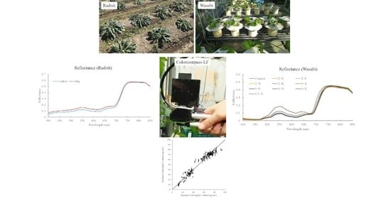
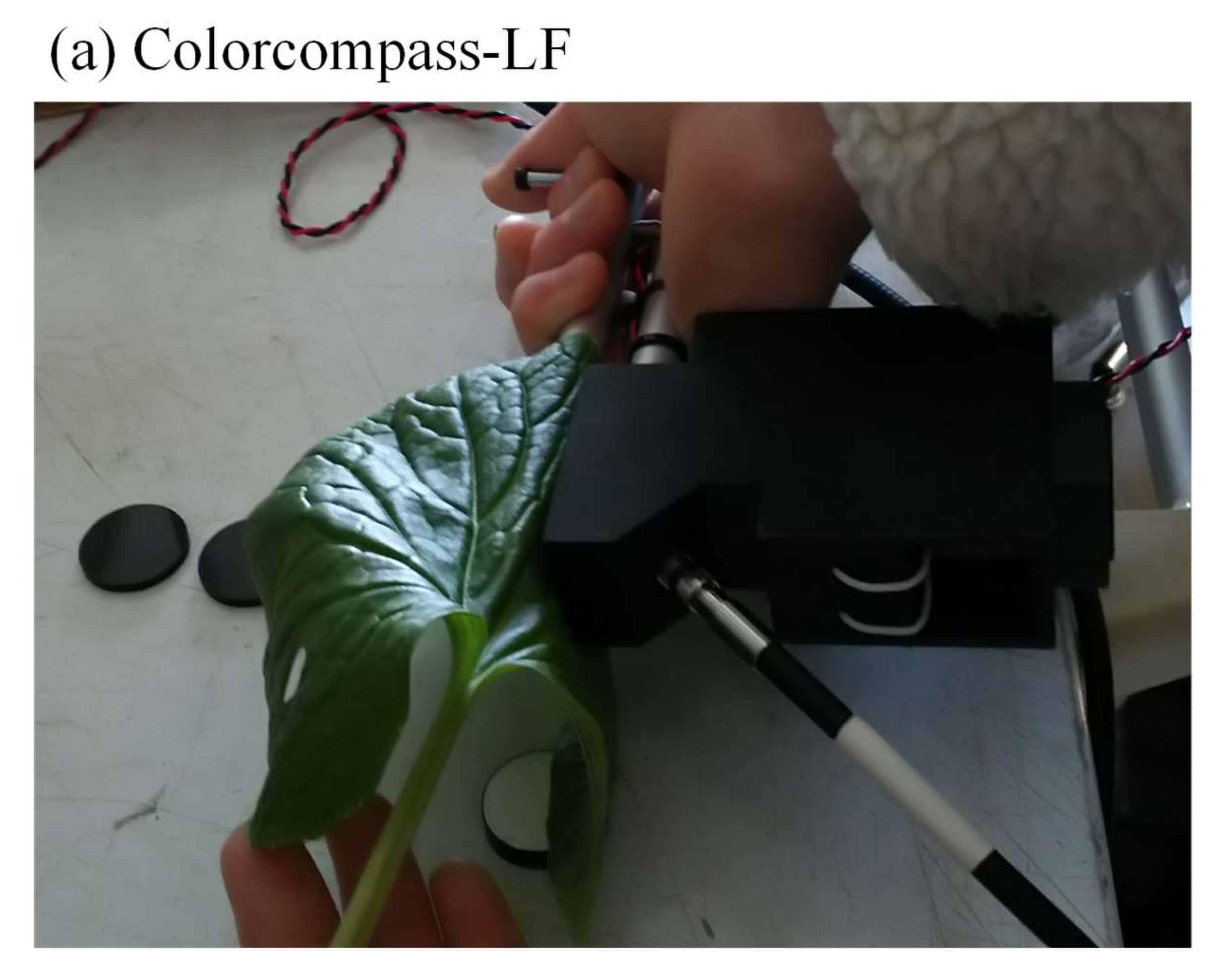
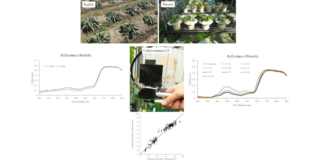
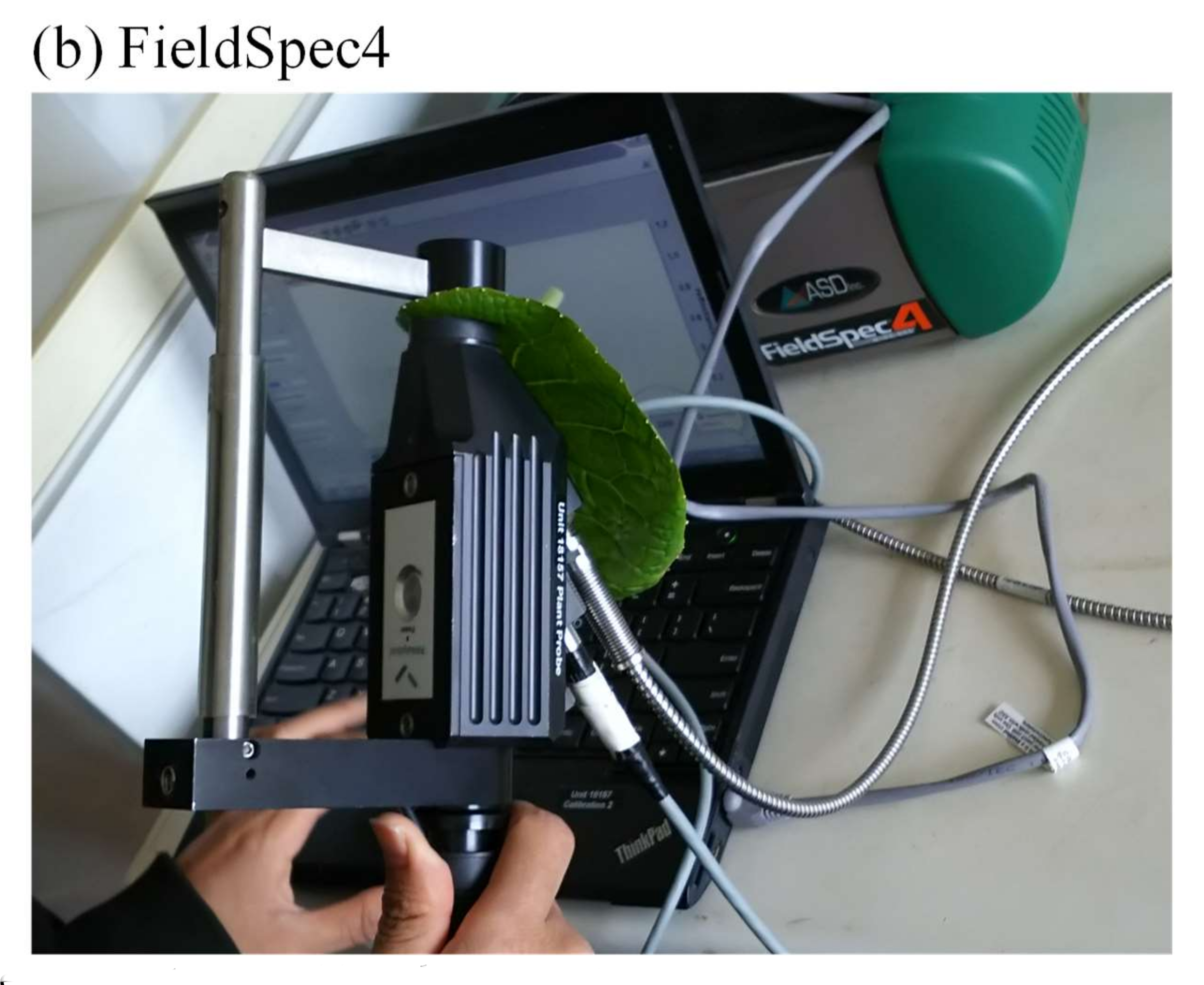
2.1. Measurements and Datasets

Two Brassicaceae species were examined in this study: radish (Raphanus sativus), which is normally cultivated in agricultural fields and has a high chlorophyll content, and wasabi (Eutrema japonicum), which is normally grown in hydroponic culture and has a relatively low chlorophyll content.

The radish plants were cultivated at a within-row distance of 60 cm and an inter-row spacing of 90 cm in a field at Shizuoka University, Japan. Basal fertiliser (6 kg of N, P and K) was applied per 10 a, in addition to 120 kg of silicate fertiliser (The Sangyo Shinko Co. Ltd., Tokyo, Japan) and 3.6 g of boric acid. The experiment included a control test without slag (control) and with slag fertilizer treatment (slag) that contained SK calcium silicate (NJ Eco Service, Kitakyushu, Japan), of which the soluble silicic acid content was 32%. Seeding was conducted on 23 October 2020, and two additional supplementary fertiliser applications were performed, consisting of 4.8 kg of N, P and K per 10 a, on 7 and 25 November. A total of 144 leaves (72 leaves per treatment) were measured for reflectance and chlorophyll content determination on 2 and 3 March 2021.

One-year-old wasabi mericlone seedlings were cultivated individually in Wagner pots (1/5000 a) containing 3 L of tap water (adjusted to a pH of 6.0 using HCl and NaOH) and were continuously aerated from 28 January 2021. After one week, slightly modified solutions of 0.1 × Hoagland solution [56] were applied stepwise for one week at a strength of 1/100 and 1/10 to adapt the plants to the hydroponic system under standard nutrient solution conditions. Hoagland solution is one of the most widely used solutions for growing plants, containing 0.25 mM KNO₃, 0.25 mM Ca (NO₃)₂4H₂O, 0.375 mM (NH₄)₂SO₄, 0.2 mM MgSO₄7H₂O, 0.2 mM NaH₂PO₄2H₂O, 0.25 mM KCl, 0.25 mM CaCl₂2H₂O, 5 μM EDTA–Fe (III), 2.5 μM H₃BO₃, 0.2 μM MnSO₄5H₂O, 0.2 μM ZnSO₄7H₂O, 0.05 μM CuSO₄5H₂O, and 0.05 μM Na₂MoO₄2H₂O. Sulphur has been reported to be important in improving the allyl isothiocyanate concentration and yield, which determine plant pungency, and sulphur is frequently added to nitrogen fertiliser [57]. Thus, sulphur was added at four concentrations: the standard concentration (control, 0.58 mM SO₄²⁻), zero sulphur (0 × S), half the standard concentration (0.5 × S), and twice the standard sulphur concentration (2 × S). Different levels of nitrogen (0 × N and 2 × N), potassium (0 × K and 2 × K), and phosphorus (0 × P and 2 × P) were added except for the control sample. A total of 100 expanding wasabi leaves (10 leaves per treatment) were sampled from the top of the plants on 16 March 2021.

For quantifying chlorophyll contents, detached leaves were used. However, the reflectance was measured immediately after detaching. Reflectance data were measured using two spectrometers with a plant probe consisting of a halogen light source and a leaf clip (Figure 1). The first spectrometer was the Colorcompass-LF, which is composed of a complementary metal–oxide semiconductor (CMOS) sensor (C12880MA-10, Hamamatsu Photonics, Hamamatsu, Japan) and a shape memory alloy (SMA) fibre patch cable (M25L05, Thorlabs, NJ, USA) with a 0.22 numerical aperture. The spectral resolution was resampled in 5 nm bands across the entire wavelength domain from 400 to 850 nm. The second spectrometer was the FieldSpec4 (Malvern Panalytical, Almelo, The Netherlands), which is composed of three detectors (visible and near-infrared [VNIR] and shortwave infrared [SWIR 1 and SWIR 2]), and the spectral drift was measured at two wavelengths (1000 nm and 1800 nm) due to inherent variations in detector sensitivities. To minimize this inconsistency, the splice correction function of ViewSpec Pro Software (Malvern Panalytical, Almelo, The Netherlands) was applied [58]. It is well known that the leaf chlorophyll content mainly affects reflectance in the 400–780 nm region [59], and the entire wavelength domain of the Colorcompass-LF spans the region from 340 nm to 850 nm. To avoid redundant analyses, reflectance values of wavelengths longer than 850 nm were removed before analysis.

Leaf discs were collected after the reflectance measurements were completed, and the absorbance of dimethyl–formamide extracts was measured using a dual-beam scanning ultraviolet–visible spectrophotometer (UV–1900, Shimadzu, Kyoto, Japan). Wellburn’s method [60] was applied to quantify the chlorophyll content based on absorption. N-N Dimethylformamide was used to prepare extracts from which chlorophyll–a (Chl–a) and b (Chl–b) contents (in μg mL⁻¹) were calculated according to the following Equations (1 to 3) with the chlorophyll unit converted to μg/cm² using the leaf disc area.

Chl–a (μg mL⁻¹) = 12.00 × (A_663.8 − A₇₅₀) − 3.11 × (A_646.8 − A₇₅₀),

(1)

Chl–b (μg mL⁻¹) = 20.78 × (A_646.8 − A₇₅₀) − 4.88 × (A_663.8 − A₇₅₀),

(2)

Chla + b (μg mL⁻¹) = Chl–a + Chl–b,

(3)

where A is the absorbance and the subscripts are the wavelengths (in nm).

A stratified random sampling approach, which is a method of sampling that involves the division of all measurements into smaller sub-groups (strata), was applied. The strata were based on treatments. The measurements were divided into two groups: a training dataset (75%) and test dataset (25%) following a previous study [49], and this approach was repeated one hundred times to ensure robust results.

2.2. Pre-Processing of the Raw Reflectance Data

Pre-processing is an essential step to remove noise from original reflectance data and to improve regression models. In this study, spectra after de-trending (DT) and standard normal variate (SNV) correction were evaluated in addition to the original reflectance (OR). DT and SNV were implemented using the “prospectr” package [61] in R version 4.0.2 [62].

2.2.1. De-Trending (DT)

In DT, the baseline is assumed to be a second-degree polynomial function of the wavelength and is subtracted from the spectrum. This technique has also been used to account for the variation in baseline shifts and curvilinearity by fitting a second-degree polynomial through each spectrum [42].

2.2.2. Standard Normal Variate (SNV)

SNV is effective in reducing multiplicative effects of scattering and particle size and is able to correct multiple scattering noise caused by the surface structure of leaves. This is mathematically expressed as follows:

$$x_{i,j}^{SNV}=\frac{x_{i,j}-\overline{x_i}}{\sqrt{\frac{{{\displaystyle \sum }}_{j=1}^p{\left(x_{i,j}-\overline{x_i}\right)}^2}{p-1}}}$$

(4)

where $x_{i,j}^{SNV}$ is the reflectance value after SNV, $x_{i,j}$ is the corresponding original reflectance value of variable j at wavelength i, $\overline{x_i}$ is the mean of spectrum i, and p is the number of variables or wavelengths in the spectrum [63].

2.3. Model Development

2.3.1. One-Dimensional Convolutional Neural Network (1D-CNN)

CNN has been applied to automatically detect features of interest from the given data, and 1D-CNN can provide accurate results for 1D data [52]; 1D-CNN has an input layer, hidden layers (convolutional, pooling, fully connected and normalization) and an output layer. Convolution was applied to the reflectance data to extract a feature map using a convolution filter, and then each unit in the convolutional layer was connected to local features in the feature map. After the convolution operation, a pooling layer was used for the dimensional reduction of the feature map, which effectively reduces the computational cost and minimises the overfitting of the network while preserving important information. In this study, the max-pooling technique and ReLU were applied. It was reported that 1D-CNN was effective to estimate the concentrations of the major and minor pigments from the reflectance and absorption coefficient spectral inputs [64]. In this study, the low and high of the chlorophyll-content samples were included and then this feature was effective for generating robust regression models. The architecture was composed of 10 hidden layers that included four convolutional layers, four max-pooling layers, and two fully connected layers; two dropout rates, 0.4 and 0.2, were used following previous studies [47,52]. The regression models based on 1D-CNN were generated using Google Colaboratory.

2.3.2. Deep Belief Nets (DBNs)

DBNs consist of multi-layer unsupervised restricted Boltzmann machines and produce an optimum model in comparison to a model based on random weights for the weight initialisation of a deep neural network [65]. DBNs can be effectively used to perform layer-by-layer pre-training intended to initialise the training of a backpropagation algorithm [66]. DBNs have been applied to extract vegetation properties, such as quality (chlorophyll-a content) and stress (chlorophyll-a: b), from hyperspectral data for improved tea tree management, and some pre-processing could be reduced [54,67]. The initial configurations were the learning rate (0.1), the maximum iteration number of the pre-training dataset (100), the learning rate of the pre-training dataset (0.01), the maximum iteration number of the training dataset (100), and the batch data size (10) following previous studies [67,68]. DBN regression was implemented using the “darch” package in R version 4.0.6 [69].

2.4. Statistical Criteria

The model performance was evaluated using the ratio of performance to deviation (RPD, Equation (5) [70]), as RPD is a widely applied indicator with a clear definition (e.g., category A [RPD > 2.0], category B [1.4 ≤ RPD ≤ 2.0], and category C [RPD < 1.4]). RPD directly compares the index performance of different datasets and is used especially to examine robustness across different datasets. In addition to RPD, the root mean square error (RMSE, Equation (6)) and coefficient of determination (R², Equation (7)) were calculated using:

$$\mathrm{RPD}=\frac{\mathrm{SD}}{\mathrm{SEP}},$$

(5)

$$\mathrm{RMSE}=\sqrt{\frac{1}{n}{\displaystyle \sum }_{i=0}^n{\left(\widehat{y_i}-y_i\right)}^2},$$

(6)

$$R^2=1-\left(\frac{{{\displaystyle \sum }}_{i=1}^n{\left(y_i-\widehat{y_i}\right)}^2}{{{\displaystyle \sum }}_{i=1}^n{\left(y_i-\overline{y}\right)}^2}\right),$$

(7)

where SD is the standard deviation of the measurements, SEP is the standard error prediction, n is the number of samples, $y_i$ is the real value, $\widehat{y_i}$ is the estimated value, and $\overline{y}$ is the mean of the measurements. Chang et al. [71] claimed that Category B can be improved by using different calibration strategies, but properties in Category C may not be reliably predicted.

The sensitivity of spectral wavelengths was evaluated using the variance principle [52,72]. For wavelength i (nm), the sensitivity S_i was calculated as follows:

$$S_i=\frac{\mathrm{Var}(f\left(X_{400},\dots ,X_i,\dots ,X_{850}\right)-f\left(\overline{X}\right)}{\mathrm{Var}\left(Y\right)},$$

(8)

where Var is the variation, f() is the prediction of spectra due to the variation in wavelength i (nm) with other wavelengths held constant at their mean values, f($\overline{X}$) is the estimated value based on the mean reflectance, and Y represents the measured chlorophyll content. Following the calculation of S_i, the scores were converted to percentages.

3. Results

3.1. Chlorophyll Contents in Each Treatment

The chlorophyll contents per leaf area (cm²) of radish were generally higher than those of wasabi and ranged from 42.20 to 94.39 μg/cm² and 11.39 to 40.40 μg/cm² for radish and wasabi, respectively (

Table 1. Chlorophyll content (μg/cm²) in each treatment.

(a) Radish
Treatment	Control	Slag	All
Number of samples	72	72	144
Minimum (μg/cm²)	43.94	42.20	42.20
Median (μg/cm²)	69.12	71.21	70.23
Mean (μg/cm²)	68.46	70.55	69.51
Maximun (μg/cm²)	94.39	92.74	94.39
Standard deviation (μg/cm²)	10.55	7.94	9.36
(b) Wasabi
Treatment	Control	0 × N	2 × N	0 × P	2 × P	0 × K	2 × K	0 × S	0.5 × S	2 × S	All
Number of samples	10	10	10	10	10	10	10	10	10	10	100
Minimum (μg/cm²)	30.89	11.39	24.02	24.60	30.55	17.96	23.99	21.17	30.12	33.08	11.39
Median (μg/cm²)	33.67	12.63	31.76	29.68	32.57	22.07	32.22	25.05	35.98	37.34	31.29
Mean (μg/cm²)	33.91	13.00	31.85	29.43	32.97	22.33	31.78	25.15	35.21	36.41	29.20
Maximun (μg/cm²)	38.82	16.11	36.87	33.37	36.56	28.94	39.18	28.97	40.40	38.93	40.40
Standard deviation (μg/cm²)	2.12	1.40	3.63	2.69	2.11	3.14	5.36	2.76	3.22	2.00	7.43

). No significant difference was observed between the two treatments for radish (p > 0.1, Tukey–Kramer test), and slag fertilizer had no effect on the chlorophyll content of the radish leaves. Except the different phosphorus fertilizer levels, the increase in the fertilizer concentrations effectively increased the chlorophyll contents.

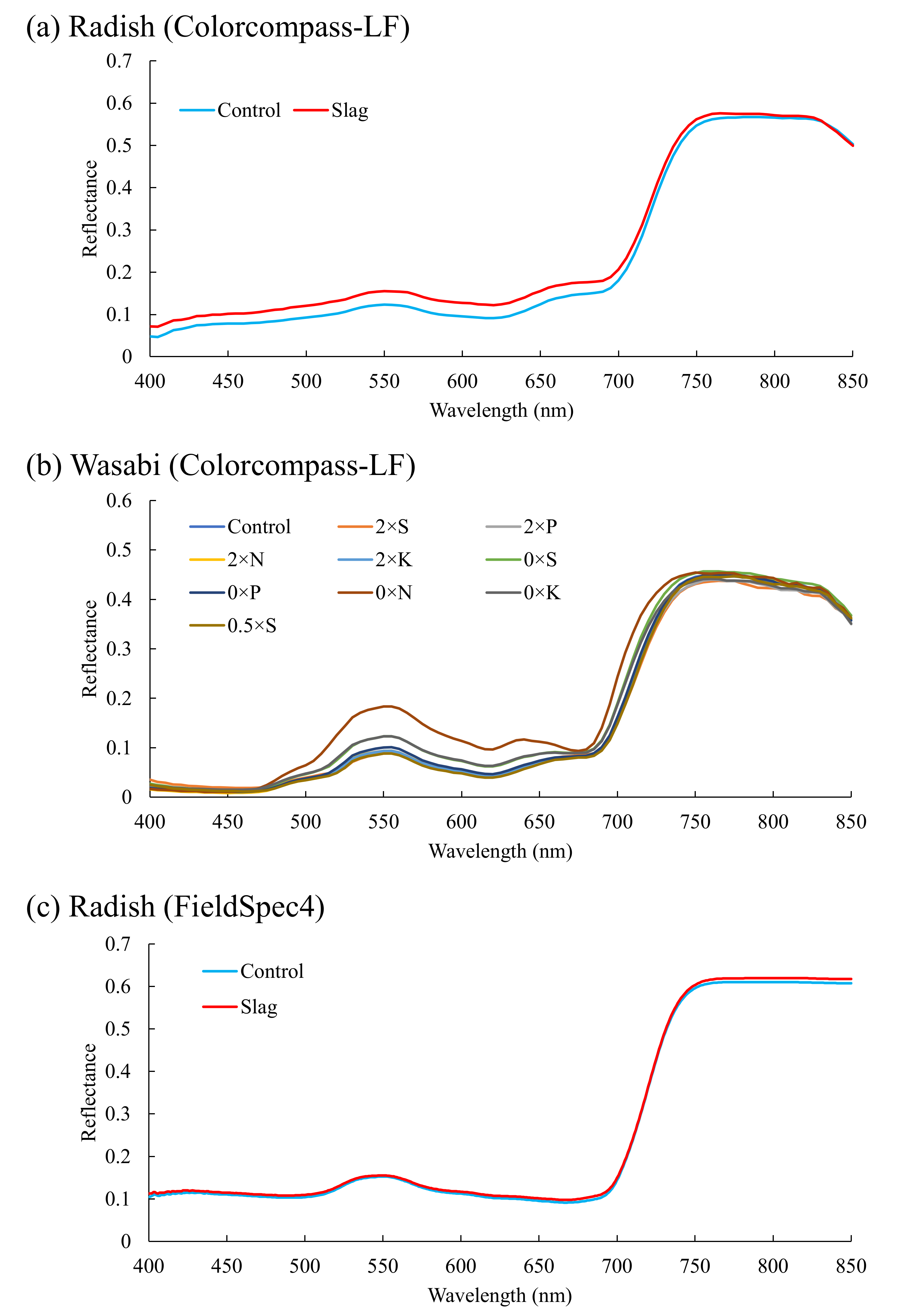
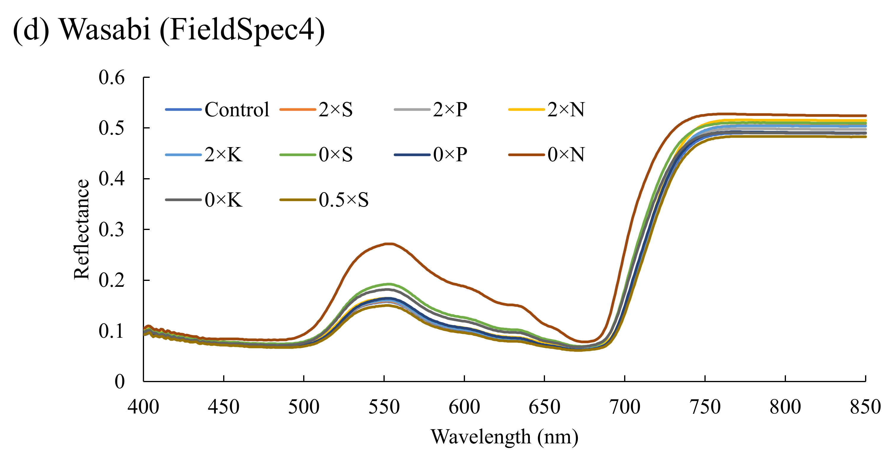
3.2. Spectral Reflectance

The mean reflectance of each crop measured by the spectrometers is shown in Figure 2. The decrease in reflectance at 825 nm was due to the low sensitivity of the C12880MA-10, which is the basis of the Colorcompass-LF. Due to high chlorophyll contents, the reflectance values in the green region were lower than those for wasabi, and high negative correlation coefficients (p < 0.001) were confirmed at 525 nm (r = −0.813 and −0.795 for the Colorcompass-LF and FieldSpec4, respectively) for wasabi. Significant negative correlations (p < 0.01) were also observed for radish; the absolute values were lower than those of wasabi (r = −0.205 and −0.391 for the Colorcompass-LF and FieldSpec4, respectively). Furthermore, strong negative correlation coefficients were observed for the red edge inflection point (REIP), and the values were −0.867 and −0.802 for the Colorcompass-LF and FieldSpec4, respectively. In contrast to the reflectance in the green region, a strong negative correlation was observed for the measurements from the FieldSpec4 (r = −0.670, p < 0.001), while a lower correlation was observed for the measurements from the Colorcompass-LF (r = −0.326, p < 0.01).

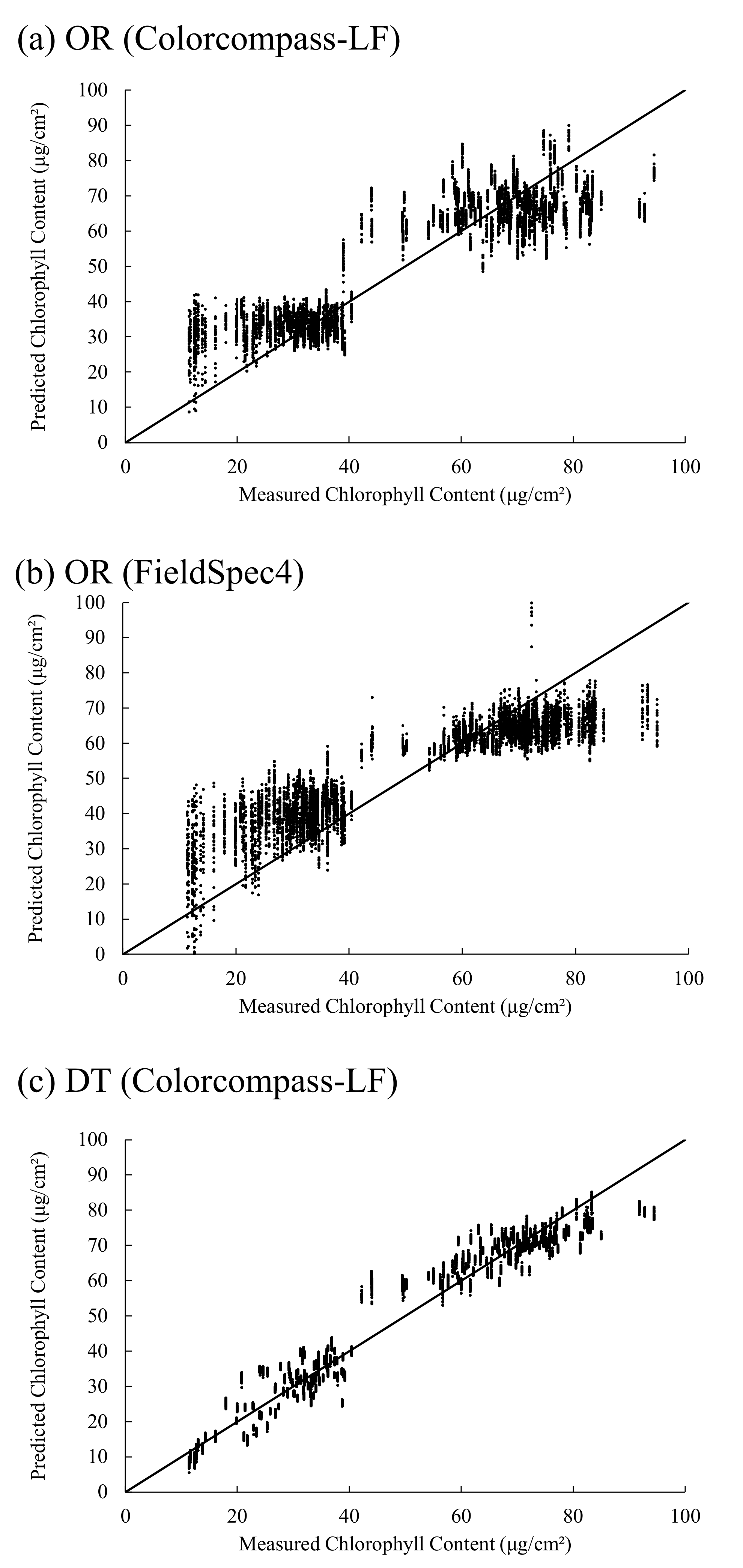
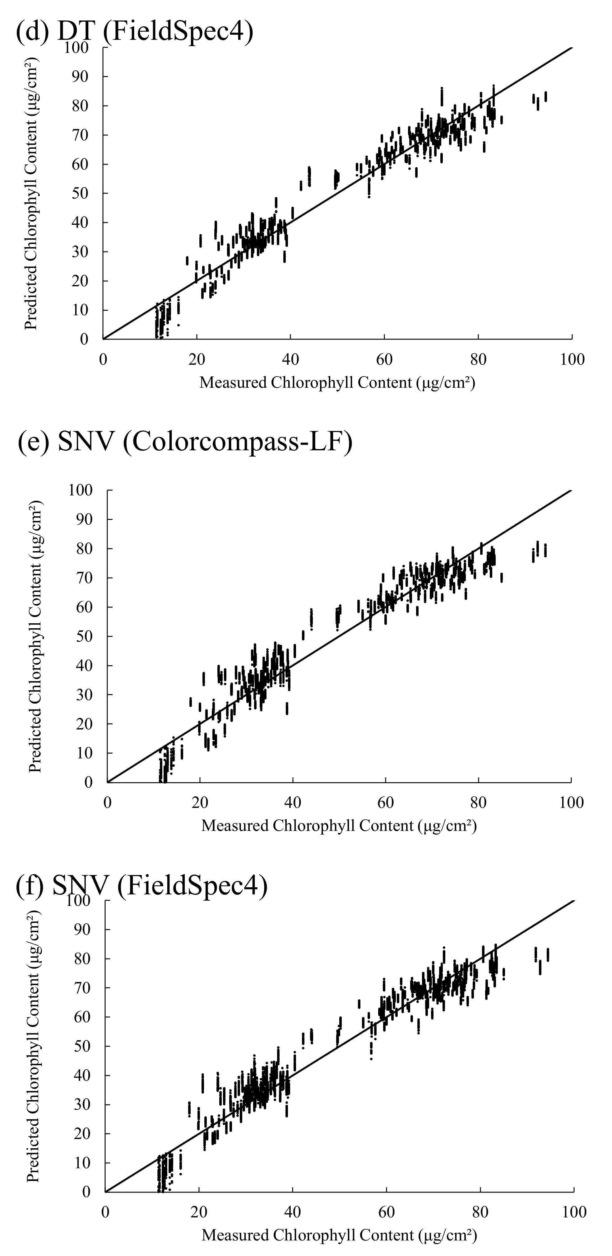
3.3. Accuracy Assessment

The evaluation results of each algorithm and pre-processing technique for measurements from both the Colorcompass-LF and FieldSpec4 are presented in

Table 2. RPD, RMSE (μg/cm²), and R² values for the estimation results for each deep learning algorithm after 100 repetitions.

(a) ColorCompass-LF
Pre-processing technique	RPD		RMSE		R²
	1D-CNN	DBN	1D-CNN	DBN	1D-CNN	DBN
OR	2.28 ± 0.37	1.44 ± 0.39	9.88 ± 1.54	16.13 ± 3.46	0.79 ± 0.06	0.43 ± 0.23
DT	4.31 ± 0.40	2.00 ± 0.63	5.13 ± 0.49	12.09 ± 3.73	0.94 ± 0.01	0.66 ± 0.21
SNV	3.70 ± 0.35	1.79 ± 0.57	5.98 ± 0.59	13.32 ± 3.72	0.92 ± 0.01	0.58 ± 0.22
(b) FieldSpec4
Pre-processing technique	RPD		RMSE		R²
	1D-CNN	DBN	1D-CNN	DBN	1D-CNN	DBN
OR	2.16 ± 0.48	1.59 ± 0.40	10.69 ± 2.44	14.60 ± 3.28	0.75 ± 0.11	0.53 ± 0.21
DT	4.33 ± 0.40	2.01 ± 0.55	5.11 ± 0.48	11.80 ± 3.42	0.94 ± 0.01	0.68 ± 0.19
SNV	4.12 ± 0.49	1.79 ± 0.46	5.40 ± 0.71	13.12 ± 3.34	0.94 ± 0.01	0.61 ± 0.22

. Although the OR of both spectrometers was acceptable for estimating the chlorophyll content (RPD > 1.4), both pre-processing techniques effectively improved the estimation accuracies and fitting of the regression models. DT was effective, and the regression models were categorised as ‘A’ (RPD > 2.0). The best combination was 1D-CNN and DT for both spectrometers, and the Colorcompass-LF had almost the same performance (RPD values) for chlorophyll content estimation (4.31 ± 0.40 μg/cm² vs. 4.33 ± 0.40 μg/cm²).

Figure 3 shows the relationships between measured and estimated values when 1D-CNN was applied. The pre-processing techniques effectively reduced the standard deviation of the estimation errors. In particular, the standard deviations of the RMSEs decreased after DT, and these values were 0.49 and 0.48 μg/cm² for the Colorcompass-LF and FieldSpec4 measurements, respectively.

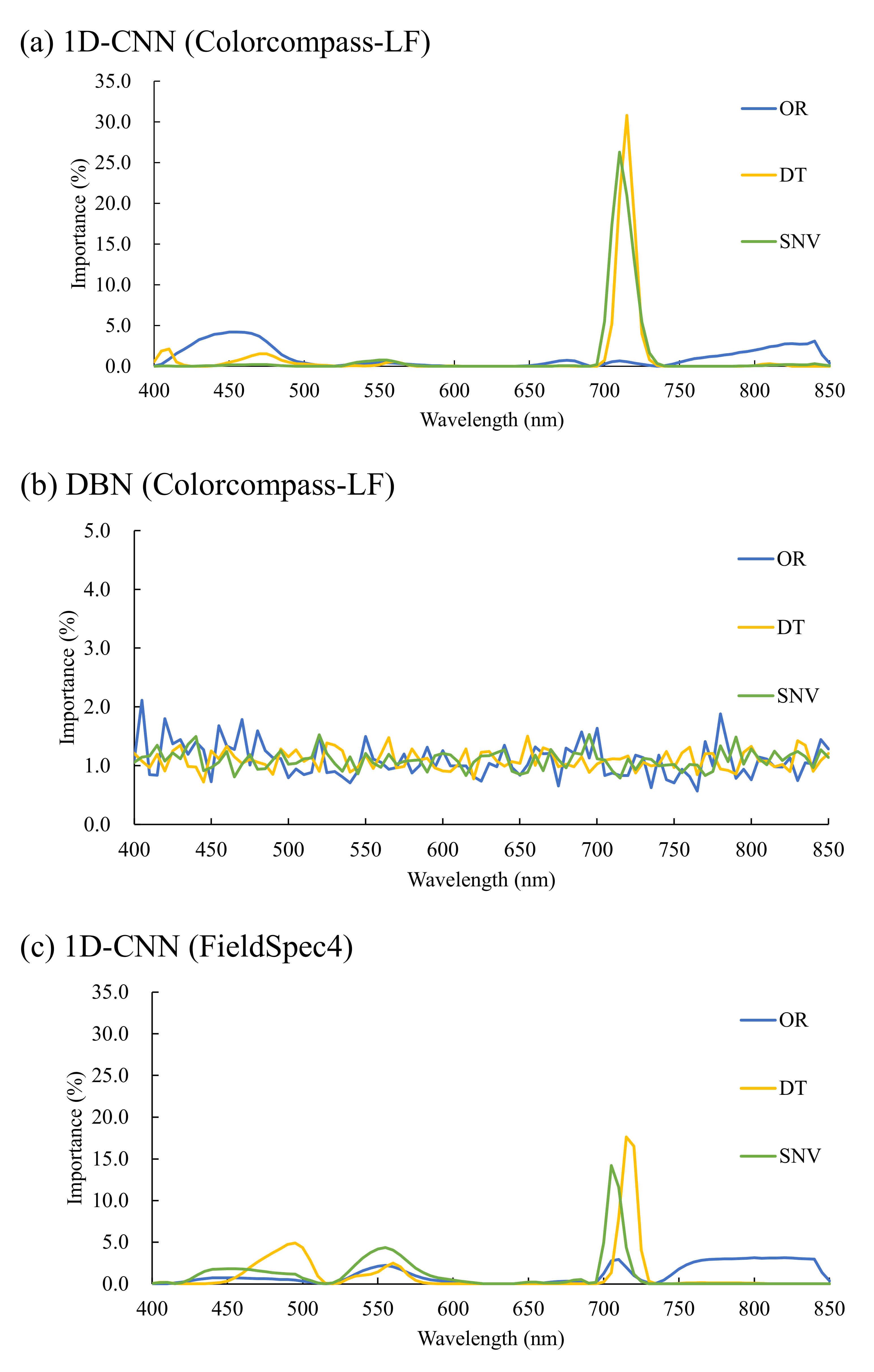
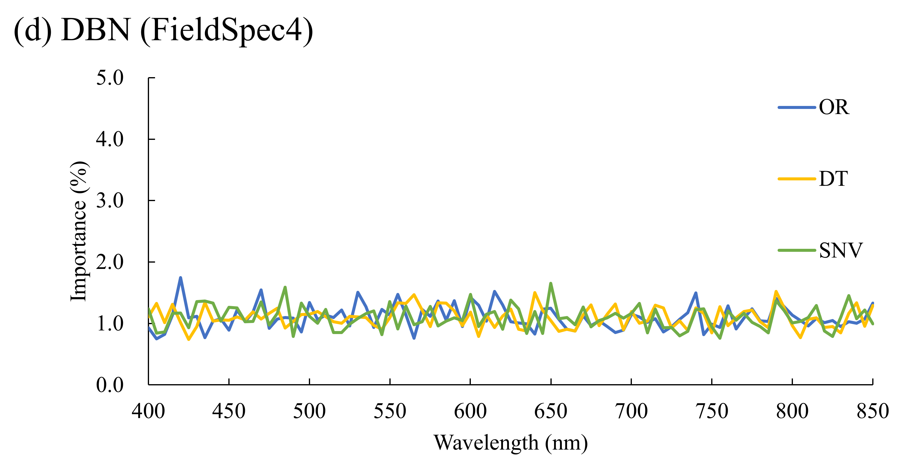
3.4. Sensitivity Analysis

Although the peaks of the importance were obscure when OR was applied, the importance of REIP for chlorophyll content estimation increased after the pre-processing techniques were applied when 1D-CNN was used (Figure 4a,c), and the most important wavelengths for DT and SNV were 710 nm and 715 nm, respectively, for Colorcompass-LF, and 720 nm and 705 nm, respectively, for FieldSpec4. The importance of the green peak was also confirmed for the FieldSpec4 measurements. On the contrary, this was not observed for DBN (Figure 4b,d).

4. Discussion

4.1. Spectrometer Comparison

When OR was applied, the estimation results from the Colorcompass-LF measurements were superior (60-fold higher) to those from the FieldSpec4. The typical FWHM wavelength of the C12880MA-10, which is the basis of the Colorcompass-LF, is 12 nm, while the FieldSpec4 has a more precise FWHM (its spectral resolution is 3 nm). Furthermore, the relative sensitivity of the C12880MA-10 is less than 0.5 at 700 nm [73]. To reduce the influence of the low sensitivity of this spectrometer, a plant probe with a halogen light source and a leaf clip with replaceable white and black background standards was developed and used in this study. FieldSpec4 is a commercial plant probe that deteriorates over time. However, pre-processing techniques were required to improve the estimation accuracies of both sensors (Table 2).

The best sensor, algorithm, and pre-processing technique combinations after 100 repetitions based on the RPD value are listed in

Table 3. The best sensor, algorithm, and pre-processing technique combinations after 100 repetitions.

Sensor	Algorithm	Pre-Processing	Times
Colorcompass-LF	1D-CNN	DT	35
		SNV	2
FieldSpec4	1D-CNN	DT	37
		SNV	26

. The estimation results from the FieldSpec4 measurements were superior (63-fold higher) to those from the Colorcompass-LF. However, the combination of 1D-CNN and DT effectively improved the chlorophyll content estimation accuracy, and the RPD values calculated from the estimation values reached 3.37–5.38 and 3.46–5.28 for the Colorcompass-LF and FieldSpec4, respectively. Therefore, it is expected that almost the same estimation accuracies can be obtained from the Colorcompass-LF measurements when 1D-CNN and DT are applied.

4.2. Optimal Machine Learning Algorithms

After 100 repetitions, 1D-CNN was included in the best combination (Table 3), and the accuracy of 1D-CNN was generally superior to that of DBN for each measurement from the sensors, although DBN had higher accuracies (6-, 2-, and 17-fold for the Colorcompass-LF original spectra, Colorcompass-LF SNV spectra, and FieldSpec4 original spectra, respectively). The minimum RPD values were 1.59, 2.87, and 1.41 for these combinations, and all estimation results were acceptable when 1D-CNN was applied. The strong performance of 1D-CNN-based regression models has been shown for soil property prediction using Vis–NIR spectral data [47,52,72], and the advantage of this algorithm was confirmed for leaf chlorophyll estimation from spectral reflectance between 400 nm and 850 nm. The important wavebands of the 1D-CNN model were also evaluated, and it was confirmed that REIP played the most important role in chlorophyll content estimation for the pre-processed spectra. The high sensitivities of the green peak have also been reported for the chlorophyll contents, and some vegetation indices based on the green peak have been proposed [22,23,74,75,76]. However, the importance of the wavelength around the green peak was low (less than 5%) for the pre-processed spectra. It has been reported that this stress moves the green peak position toward long wavelengths [77], and the nutrient content in the Wagner pots may have influenced the water status of the cultivated wasabi plants. However, the REIPs of the mean spectra ranged from 710 nm to 715 nm (for both spectrometers) while the green peak ranged from 520 nm to 530 nm for the Colorcompass-LF measurements and was 520 nm for the FieldSpec4 measurements. As a result, there were no large shifts for the two bands. It has been reported that anthocyanin induction is strongly influenced by a low nitrogen concentration, and the absorption peak of anthocyanin corresponds to the green peak region, but there is no influence on the red edge region [78]. Therefore, REIP had relatively high sensitivities in the regression models. In future measurements, assessments of the influence of anthocyanin contents should be considered. The tendencies of important wavelengths were obscure for both spectrometer measurements when DBN was applied, as observed in results of previous studies, and this tendency is important for processing the spectra, including noise reduction [43,67]. Indeed, the application of the pre-processing techniques was less effective (Table 2); however, the performances were lower than those of the 1D-CNN-based regression models, even for the original reflectance.

5. Conclusions

In this study, hyperspectral data were acquired using a low-cost complementary metal–oxide semiconductor (CMOS) sensor, Colorcompass-LF, and an Analytical Spectral Devices (ASD) FieldSpec4 to evaluate the performance of the Colorcompass-LF.

De-trending based on a second-degree polynomial effectively removed noise from the Colorcompass-LF and FieldSpec4 measurements, and the relative percent difference values reached 3–4 when one-dimensional convolutional neural network-based regression models were applied. As a result, the low-cost reflectance measurement system (Colorcompass-LF) estimates the chlorophyll content with almost the same accuracy as the high-specification spectrometer (ASD FieldSpec4). The information provided by the Colorcompass-LF can be used for more suitable nutrient management, facilitating quality control and plant maintenance for less-experienced farmers with low-cost field-scale monitoring.

References

1. Wang, Y.; Jia, B.Y.; Ren, H.J.; Feng, Z. Ploidy level enhances the photosynthetic capacity of a tetraploid variety of Acer buergerianum Miq. Peerj 2021, 9, e12620. [Google Scholar] [CrossRef] [PubMed]
2. Krizova, K.; Kaderabek, J.; Novak, V.; Linda, R.; Kuresova, G.; Sarec, P. Using a single-board computer as a low-cost instrument for SPAD value estimation through colour images and chlorophyll-related spectral indices. Ecol. Inform. 2022, 67, 101496. [Google Scholar] [CrossRef]
3. Chen, N.L.; Tang, R.Y.; Zhang, Y.X.; An, C.X.; Gao, H.J. Photosynthetic and Biochemical Changes of Melon Leaves during Senescence. Iv Int. Symp. Cucurbits 2010, 871, 329–336. [Google Scholar]
4. Yamamoto, A.; Nakamura, T.; Adu-Gyamfi, J.J.; Saigusa, M. Relationship between chlorophyll content in leaves of sorghum and pigeonpea determined by extraction method and by chlorophyll meter (SPAD-502). J. Plant Nutr. 2002, 25, 2295–2301. [Google Scholar] [CrossRef]
5. Peng, S.B.; Garcia, F.V.; Laza, R.C.; Cassman, K.G. Adjustment for Specific Leaf Weight Improves Chlorophyll Meter’s Estimate of Rice Leaf Nitrogen Concentration. Agron. J. 1993, 85, 987–990. [Google Scholar] [CrossRef]
6. Gautam, D.; Lucieer, A.; Watson, C.; McCoull, C. Lever-arm and boresight correction, and field of view determination of a spectroradiometer mounted on an unmanned aircraft system. ISPRS J. Photogramm. Remote Sens. 2019, 155, 25–36. [Google Scholar] [CrossRef]
7. Zarco-Tejada, P.J.; Berjon, A.; Lopez-Lozano, R.; Miller, J.R.; Martin, P.; Cachorro, V.; Gonzalez, M.R.; de Frutos, A. Assessing vineyard condition with hyperspectral indices: Leaf and canopy reflectance simulation in a row-structured discontinuous canopy. Remote Sens. Environ. 2005, 99, 271–287. [Google Scholar] [CrossRef]
8. Feret, J.B.; Francois, C.; Asner, G.P.; Gitelson, A.A.; Martin, R.E.; Bidel, L.P.R.; Ustin, S.L.; le Maire, G.; Jacquemoud, S. PROSPECT-4 and 5: Advances in the leaf optical properties model separating photosynthetic pigments. Remote Sens. Environ. 2008, 112, 3030–3043. [Google Scholar] [CrossRef]
9. Nofrizal, A.Y.; Sonobe, R.; Yamashita, H.; Ikka, T.I.; Morita, A. Estimation of chlorophyll content in radish leaves using hyperspectral remote sensing data and machine learning algorithms. In Proceedings of the Remote Sensing for Agriculture, Ecosystems, and Hydrology XXIII, Andalusia, Spain, 13–18 September 2021. [Google Scholar]
10. Sonobe, R.; Sugimoto, Y.; Kondo, R.; Seki, H.; Sugiyama, E.; Kiriiwa, Y.; Suzuki, K. Hyperspectral wavelength selection for estimating chlorophyll content of muskmelon leaves. Eur. J. Remote Sens. 2021, 54, 512–523. [Google Scholar] [CrossRef]
11. El-Hendawy, S.; Dewir, Y.H.; Elsayed, S.; Schmidhalter, U.; Al-Gaadi, K.; Tola, E.; Refay, Y.; Tahir, M.U.; Hassan, W.M. Combining Hyperspectral Reflectance Indices and Multivariate Analysis to Estimate Different Units of Chlorophyll Content of Spring Wheat under Salinity Conditions. Plants 2022, 11, 456. [Google Scholar] [CrossRef]
12. Blackburn, G.A. Quantifying chlorophylls and caroteniods at leaf and canopy scales: An evaluation of some hyperspectral approaches. Remote Sens. Environ. 1998, 66, 273–285. [Google Scholar] [CrossRef]
13. Blackburn, G.A. Spectral indices for estimating photosynthetic pigment concentrations: A test using senescent tree leaves. Int. J. Remote Sens. 1998, 19, 657–675. [Google Scholar] [CrossRef]
14. Gandia, S.; Fernández, G.; Moreno, J. Retrieval of Vegetation Biophysical Variables from CHRIS/PROBA Data in the SPARC Campaign. In Proceedings of the the 2nd CHRIS/Proba Workshop, Frascati, Italy, 28–30 April 2004; pp. 40–48. [Google Scholar]
15. Gitelson, A.; Merzlyak, M.N. Spectral reflectance changes associated with autumn senescence of Aesculus hippocastanum L. and Acer platanoides L. Leaves. Spectral features and relation to chlorophyll estimation. J. Plant Physiol. 1994, 143, 286–292. [Google Scholar] [CrossRef]
16. Le Maire, G.; Francois, C.; Soudani, K.; Berveiller, D.; Pontailler, J.-Y.; Breda, N.; Genet, H.; Davi, H.; Dufrene, E. Calibration and validation of hyperspectral indices for the estimation of broadleaved forest leaf chlorophyll content, leaf mass per area, leaf area index and leaf canopy biomass. Remote Sens. Environ. 2008, 112, 3846–3864. [Google Scholar] [CrossRef]
17. Sims, D.A.; Gamon, J.A. Relationships between leaf pigment content and spectral reflectance across a wide range of species, leaf structures and developmental stages. Remote Sens. Environ. 2002, 81, 337–354. [Google Scholar] [CrossRef]
18. Tanaka, S.; Kawamura, K.; Maki, M.; Muramoto, Y.; Yoshida, K.; Akiyama, T. Spectral Index for Quantifying Leaf Area Index of Winter Wheat by Field Hyperspectral Measurements: A Case Study in Gifu Prefecture, Central Japan. Remote Sens. 2015, 7, 5329–5346. [Google Scholar] [CrossRef] [Green Version]
19. Sonobe, R.; Wang, Q. Assessing the xanthophyll cycle in natural beech leaves with hyperspectral reflectance. Funct. Plant Biol. 2016, 43, 438–447. [Google Scholar] [CrossRef]
20. Carter, G.A. Ratios of leaf reflectances in narrow wavebands as indicators of plant stress. Int. J. Remote Sens. 1994, 15, 697–703. [Google Scholar] [CrossRef]
21. Carter, G.A.; Knapp, A.K. Leaf optical properties in higher plants: Linking spectral characteristics to stress and chlorophyll concentration. Am. J. Bot. 2001, 88, 677–684. [Google Scholar] [CrossRef] [Green Version]
22. Chappelle, E.W.; Kim, M.S.; McMurtrey, J.E. Ratio analysis of reflectance spectra (RARS): An algorithm for the remote estimation of the concentrations of chlorophyll A, chlorophyll B, and carotenoids in soybean leaves. Remote Sens. Environ. 1992, 39, 239–247. [Google Scholar] [CrossRef]
23. Datt, B. Remote sensing of chlorophyll a, chlorophyll b, chlorophyll a+b, and total carotenoid content in eucalyptus leaves. Remote Sens. Environ. 1998, 66, 111–121. [Google Scholar] [CrossRef]
24. Datt, B. A new reflectance index for remote sensing of chlorophyll content in higher plants: Tests using Eucalyptus leaves. J. Plant Physiol. 1999, 154, 30–36. [Google Scholar] [CrossRef]
25. Datt, B. Visible/near infrared reflectance and chlorophyll content in Eucalyptus leaves. Int. J. Remote Sens. 1999, 20, 2741–2759. [Google Scholar] [CrossRef]
26. Gitelson, A.A.; Merzlyak, M.N. Signature analysis of leaf reflectance spectra: Algorithm development for remote sensing of chlorophyll. J. Plant Physiol. 1996, 148, 494–500. [Google Scholar] [CrossRef]
27. Jordan, C.F. Derivation of leaf-area index from quality of light on the forest floor. Ecology 1969, 50, 663–666. [Google Scholar] [CrossRef]
28. Lichtenthaler, H.K.; Lang, M.; Sowinska, M.; Heisel, F.; Miehe, J.A. Detection of vegetation stress via a new high resolution fluorescence imaging system. J. Plant Physiol. 1996, 148, 599–612. [Google Scholar] [CrossRef]
29. McMurtrey, J.E.; Chappelle, E.W.; Kim, M.S.; Meisinger, J.J.; Corp, L.A. Distinguishing nitrogen fertilization levels in field corn (Zea mays L.) with actively induced fluorescence and passive reflectance measurements. Remote Sens. Environ. 1994, 47, 36–44. [Google Scholar] [CrossRef]
30. Penuelas, J.; Filella, I.; Biel, C.; Serrano, L.; Save, R. The reflectance at the 950?970 nm region as an indicator of plant water status. Int. J. Remote Sens. 1993, 14, 1887–1905. [Google Scholar] [CrossRef]
31. Smith, R.C.G.; Adams, J.; Stephens, D.J.; Hick, P.T. Forecasting wheat yield in a Mediterranean-type environment from the NOAA satellite. Aust. J. Agric. Res. 1995, 46, 113–125. [Google Scholar] [CrossRef]
32. Vogelmann, J.E.; Rock, B.N.; Moss, D.M. Red edge spectral measurements from sugar maple leaves. Int. J. Remote Sens. 1993, 14, 1563–1575. [Google Scholar] [CrossRef]
33. Zarco-Tejada, P.J.; Miller, J.R.; Haboudane, D.; Tremblay, N.; Apostol, S. Detection of chlorophyll fluorescence in vegetation from airborne hyperspectral CASI imagery in the red edge spectral region. In Proceedings of the International Geoscience and Remote Sensing Symposium (IGARSS), Toulouse, France, 21–25 July 2003; pp. 598–600. [Google Scholar]
34. Zarco-Tejada, P.J.; Pushnik, J.C.; Dobrowski, S.; Ustin, S.L. Steady-state chlorophyll a fluorescence detection from canopy derivative reflectance and double-peak red-edge effects. Remote Sens. Environ. 2003, 84, 283–294. [Google Scholar] [CrossRef]
35. Sonobe, R.; Yamaya, Y.; Tani, H.; Wang, X.F.; Kobayashi, N.; Mochizuki, K. Crop classification from Sentinel-2-derived vegetation indices using ensemble learning. J. Appl. Remote Sens. 2018, 12, 026019. [Google Scholar] [CrossRef] [Green Version]
36. Li, Z.H.; Jin, X.L.; Wang, J.H.; Yang, G.J.; Nie, C.W.; Xu, X.G.; Feng, H.K. Estimating winter wheat (Triticum aestivum) LAI and leaf chlorophyll content from canopy reflectance data by integrating agronomic prior knowledge with the PROSAIL model. Int. J. Remote Sens. 2015, 36, 2634–2653. [Google Scholar] [CrossRef]
37. Masemola, C.; Cho, M.A.; Ramoelo, A. Comparison of Landsat 8 OLI and Landsat 7 ETM+ for estimating grassland LAI using model inversion and spectral indices: Case study of Mpumalanga, South Africa. Int. J. Remote Sens. 2016, 37, 4401–4419. [Google Scholar] [CrossRef]
38. Uto, K.; Seki, H.; Saito, G.; Kosugi, Y.; Komatsu, T. Development of a Low-Cost Hyperspectral Whiskbroom Imager Using an Optical Fiber Bundle, a Swing Mirror, and Compact Spectrometers. IEEE J. Sel. Top. Appl. Earth Obs. Remote Sens. 2016, 9, 3909–3925. [Google Scholar] [CrossRef]
39. Song, B.W.; Liu, L.Y.; Zhang, B. A novel restoration approach for vegetation reflectance spectra at noisy bands using the principal component analysis method. Int. J. Remote Sens. 2020, 41, 2303–2325. [Google Scholar] [CrossRef]
40. Huang, Z.Q.; Huang, W.X.; Li, S.; Ni, B.; Zhang, Y.L.; Wang, M.W.; Chen, M.L.; Zhu, F.X. Inversion Evaluation of Rare Earth Elements in Soil by Visible-Shortwave Infrared Spectroscopy. Remote Sens. 2021, 13, 4886. [Google Scholar] [CrossRef]
41. Ducasse, E.; Adeline, K.; Briottet, X.; Hohmann, A.; Bourguignon, A.; Grandjean, G. Montmorillonite Estimation in Clay-Quartz-Calcite Samples from Laboratory SWIR Imaging Spectroscopy: A Comparative Study of Spectral Preprocessings and Unmixing Methods. Remote Sens. 2020, 12, 1723. [Google Scholar] [CrossRef]
42. Barnes, R.J.; Dhanoa, M.S.; Lister, S.J. Standard Normal Variate Transformation and De-Trending of Near-Infrared Diffuse Reflectance Spectra. Appl. Spectrosc. 1989, 43, 772–777. [Google Scholar] [CrossRef]
43. Sonobe, R.; Yamashita, H.; Mihara, H.; Morita, A.; Ikka, T. Hyperspectral reflectance sensing for quantifying leaf chlorophyll content in wasabi leaves using spectral pre-processing techniques and machine learning algorithms. Int. J. Remote Sens. 2021, 42, 1311–1329. [Google Scholar] [CrossRef]
44. Sonobe, R.; Yamashita, H.; Mihara, H.; Morita, A.; Ikka, T. Estimation of Leaf Chlorophyll a, b and Carotenoid Contents and Their Ratios Using Hyperspectral Reflectance. Remote Sens. 2020, 12, 3265. [Google Scholar] [CrossRef]
45. Yamashita, H.; Sonobe, R.; Hirono, Y.; Morita, A.; Ikka, T. Dissection of hyperspectral reflectance to estimate nitrogen and chlorophyll contents in tea leaves based on machine learning algorithms. Sci. Rep. 2020, 10, 17360. [Google Scholar] [CrossRef] [PubMed]
46. Liang, K.; Huang, J.N.; He, R.Y.; Wang, Q.J.; Chai, Y.Y.; Shen, M.X. Comparison of Vis-NIR and SWIR hyperspectral imaging for the non-destructive detection of DON levels in Fusarium head blight wheat kernels and wheat flour. Infrared Phys. Technol. 2020, 106, 103281. [Google Scholar] [CrossRef]
47. Kawamura, K.; Nishigaki, T.; Andriamananjara, A.; Rakotonindrina, H.; Tsujimoto, Y.; Moritsuka, N.; Rabenarivo, M.; Razafimbelo, T. Using a One-Dimensional Convolutional Neural Network on Visible and Near-Infrared Spectroscopy to Improve Soil Phosphorus Prediction in Madagascar. Remote Sens. 2021, 13, 1519. [Google Scholar] [CrossRef]
48. Brunet, D.; Barthes, B.G.; Chotte, J.L.; Feller, C. Determination of carbon and nitrogen contents in Alfisols, Oxisols and Ultisols from Africa and Brazil using NIRS analysis: Effects of sample grinding and set heterogeneity. Geoderma 2007, 139, 106–117. [Google Scholar] [CrossRef]
49. Pullanagari, R.R.; Dehghan-Shoar, M.; Yule, I.J.; Bhatia, N. Field spectroscopy of canopy nitrogen concentration in temperate grasslands using a convolutional neural network. Remote Sens. Environ. 2021, 257, 112353. [Google Scholar] [CrossRef]
50. Chu, H.J.; Zhang, C.; Wang, M.C.; Gouda, M.; Wei, X.H.; He, Y.; Liu, Y.F. Hyperspectral imaging with shallow convolutional neural networks (SCNN) predicts the early herbicide stress in wheat cultivars. J. Hazard. Mater. 2022, 421, 126706. [Google Scholar] [CrossRef]
51. Jiang, X.F.; Duan, H.C.; Liao, J.; Guo, P.L.; Huang, C.H.; Xue, X. Estimation of Soil Salinization by Machine Learning Algorithms in Different Arid Regions of Northwest China. Remote Sens. 2022, 14, 347. [Google Scholar] [CrossRef]
52. Ng, W.; Minasny, B.; Montazerolghaem, M.; Padarian, J.; Ferguson, R.; Bailey, S.; McBratney, A.B. Convolutional neural network for simultaneous prediction of several soil properties using visible/near-infrared, mid-infrared, and their combined spectra. Geoderma 2019, 352, 251–267. [Google Scholar] [CrossRef]
53. Chen, J.H.; Zhao, Z.Q.; Shi, J.Y.; Zhao, C. A New Approach for Mobile Advertising Click-Through Rate Estimation Based on Deep Belief Nets. Comput. Intell. Neurosci. 2017, 2017, 7259762. [Google Scholar] [CrossRef] [Green Version]
54. Sonobe, R.; Hirono, Y.; Oi, A. Quantifying chlorophyll-a and b content in tea leaves using hyperspectral reflectance and deep learning. Remote Sens. Lett. 2020, 11, 933–942. [Google Scholar] [CrossRef]
55. Chen, Y.S.; Lin, Z.H.; Zhao, X.; Wang, G.; Gu, Y.F. Deep Learning-Based Classification of Hyperspectral Data. Ieee J. Sel. Top. Appl. Earth Obs. Remote Sens. 2014, 7, 2094–2107. [Google Scholar] [CrossRef]
56. Hoagland, D.R.; Arnon, D.I. The water-culture method for growing plants without soil. Circular 1938, 347, 1884–1949. [Google Scholar]
57. Sultana, T.; Savage, G.P.; McNeil, D.L.; Porter, N.G.; Martin, R.J.; Deo, B. Effects of fertilisation on the allyl isothiocyanate profile of above-ground tissues of New Zealand-grown wasabi. J. Sci. Food Agric. 2002, 82, 1477–1482. [Google Scholar] [CrossRef]
58. Prasad, K.A.; Gnanappazham, L.; Selvam, V.; Ramasubramanian, R.; Kar, C.S. Developing a spectral library of mangrove species of Indian east coast using field spectroscopy. Geocarto Int. 2015, 30, 580–599. [Google Scholar] [CrossRef]
59. Feret, J.B.; Gitelson, A.A.; Noble, S.D.; Jacquemoud, S. PROSPECT-D: Towards modeling leaf optical properties through a complete lifecycle. Remote Sens. Environ. 2017, 193, 204–215. [Google Scholar] [CrossRef] [Green Version]
60. Wellburn, A.R. The spectral determination of chlorophyll a and chlorophyll b, as well as total carotenoids, using various solvents with spectrophotometers of different resolution. J. Plant Physiol. 1994, 144, 307–313. [Google Scholar] [CrossRef]
61. Stevens, A.; Ramirez-Lopez, L. Package ‘Prospectr’. Available online: https://cran.r-project.org/web/packages/prospectr/prospectr.pdf (accessed on 18 March 2022).
62. R Core Team. R: A language and environment for statistical computing. R Foundation for Statistical Computing. Available online: https://www.R-project.org/ (accessed on 18 March 2022).
63. Brown, S.; Tauler, R.; Walczak, B. (Eds.) Comprehensive Chemometrics: Chemical and Biochemical Data Analysis, Vols 1-4; Elsevier: Amsterdam, The Netherlands, 2009. [Google Scholar]
64. Pyo, J.; Hong, S.M.; Jang, J.; Park, S.; Park, J.; Noh, J.H.; Cho, K.H. Drone-borne sensing of major and accessory pigments in algae using deep learning modeling. Giscience Remote Sens. 2022, 59, 310–332. [Google Scholar] [CrossRef]
65. Hinton, G.E.; Osindero, S.; Teh, Y.W. A fast learning algorithm for deep belief nets. Neural Comput. 2006, 18, 1527–1554. [Google Scholar] [CrossRef]
66. Ghasemi, F.; Mehridehnavi, A.; Fassihi, A.; Perez-Sanchez, H. Deep neural network in QSAR studies using deep belief network. Appl. Soft Comput. 2018, 62, 251–258. [Google Scholar] [CrossRef]
67. Sonobe, R.; Hirono, Y.; Oi, A. Non-Destructive Detection of Tea Leaf Chlorophyll Content Using Hyperspectral Reflectance and Machine Learning Algorithms. Plants 2020, 9, 368. [Google Scholar] [CrossRef] [PubMed] [Green Version]
68. Du, J.L.; Liu, Y.Y.; Liu, Z.J. Study of Precipitation Forecast Based on Deep Belief Networks. Algorithms 2018, 11, 132. [Google Scholar] [CrossRef] [Green Version]
69. Drees, M.; Rueckert, J.; Hinton, G.; Salakhutdinov, R.; Rasmussen, C.E. Package for Deep Architectures and Restricted Boltzmann Machines. Available online: https://mran.microsoft.com/snapshot/2016-07-08/web/packages/darch/darch.pdf (accessed on 18 March 2022).
70. Williams, P. Variables affecting near-infraredreflectance spectroscopic analysis. In Near-Infrared Technology in the Agricultural and Food Industries; Williams, P., Norris, K., Eds.; American Association of Cereal Chemists Inc.: Eagan, MI, USA, 1987; pp. 143–167. [Google Scholar]
71. Chang, C.W.; Laird, D.A.; Mausbach, M.J.; Hurburgh, C.R. Near-infrared reflectance spectroscopy-principal components regression analyses of soil properties. Soil Sci. Soc. Am. J. 2001, 65, 480–490. [Google Scholar] [CrossRef] [Green Version]
72. Ng, W.; Minasny, B.; Mendes, W.D.; Dematt, J.A.M. The influence of training sample size on the accuracy of deep learning models for the prediction of soil properties with near-infrared spectroscopy data. Soil 2020, 6, 565–578. [Google Scholar] [CrossRef]
73. Hamamatsu Photonics. Mini-Spectrometer. Available online: http://www.farnell.com/datasheets/2822646.pdf (accessed on 18 March 2022).
74. Gitelson, A.A.; Zur, Y.; Chivkunova, O.B.; Merzlyak, M.N. Assessing carotenoid content in plant leaves with reflectance spectroscopy. Photochem. Photobiol. 2002, 75, 272–281. [Google Scholar] [CrossRef]
75. Hernandez-Clemente, R.; Navarro-Cerrillo, R.M.; Zarco-Tejada, P.J. Carotenoid content estimation in a heterogeneous conifer forest using narrow-band indices and PROSPECT plus DART simulations. Remote Sens. Environ. 2012, 127, 298–315. [Google Scholar] [CrossRef]
76. Sonobe, R.; Wang, Q. Nondestructive assessments of carotenoids content of broadleaved plant species using hyperspectral indices. Comput. Electron. Agric. 2018, 145, 18–26. [Google Scholar] [CrossRef]
77. Feng, R.; Wu, J.W.; Wang, H.B.; Hu, W.; Zhang, Y.S.; Yu, W.Y.; Ji, R.P.; Lin, Y. Influence of Drought Stress on Maize in the Seedling Stage on Spectral Characteristics at the Critical Developmental Stage. Spectrosc. Spectr. Anal. 2020, 40, 2222–2228. [Google Scholar] [CrossRef]
78. Gitelson, A.A.; Keydan, G.P.; Merzlyak, M.N. Three-band model for noninvasive estimation of chlorophyll, carotenoids, and anthocyanin contents in higher plant leaves. Geophys. Res. Lett. 2006, 33, L11402. [Google Scholar] [CrossRef] [Green Version]
Figure 1. Measurements of the chlorophyll content of wasabi leaves using (a) the Colorcompass-LF and (b) the FieldSpec4.
Remotesensing 14 01997 g001aRemotesensing 14 01997 g001b
Figure 2. Mean reflectance spectra measured by the Colorcompass-LF ((a) radish, (b) wasabi) and FieldSpec4 ((c) radish, (d) wasabi).
Remotesensing 14 01997 g002aRemotesensing 14 01997 g002b
Figure 3. Relationship between measured and estimated chlorophyll contents using (a) OR of Colorcompass-LF, (b) OR of FieldSpec4, (c) DT of Colorcompass-LF, (d) DT of FieldSpec4, and (e) SNV of Colorcompass-LF, (f) SNV of FieldSpec4.
Remotesensing 14 01997 g003aRemotesensing 14 01997 g003b
Figure 4. Sensitivity analysis results for the combinations of algorithms and spectrometers for the combinations of (a) 1D-CNN and reflectance from Colorcompass-LF, (b) DBN and reflectance from Colorcompass-LF, (c) 1D-CNN and reflectance from FieldSpec4, and (d) DBN and reflectance from FieldSpec4.
Remotesensing 14 01997 g004aRemotesensing 14 01997 g004b