Abstract
In near-field remote sensing, noncontact methods (radars) that measure stage and surface water velocity have the potential to supplement traditional bridge scour monitoring tools because they are safer to access and are less likely to be damaged compared with in-stream sensors. The objective of this study was to evaluate the use of radars for monitoring the hydraulic conditions that contribute to bridge–pier scour in gravel-bed channels. Measurements collected with a radar were also leveraged along with minimal field measurements to evaluate whether time-integrated stream power per unit area (Ω) was correlated with observed scour depth at a scour-critical bridge in Colorado. The results of this study showed that (1) there was close agreement between radar-based and U.S. Geological Survey streamgage-based measurements of stage and discharge, indicating that radars may be viable tools for monitoring flow conditions that lead to bridge pier scour; (2) Ω and pier scour depth were correlated, indicating that radar-derived Ω measurements may be used to estimate scour depth in real time and predict scour depth based on the measured trajectory of Ω. The approach presented in this study is intended to supplement, rather than replace, existing high-fidelity scour monitoring techniques and provide data quickly in information-poor areas.
Keywords:
radar; noncontact; bridge scour; stream power; discharge; velocity; river; probability concept 1. Introduction
Federal and state transportation departments are responsible for maintaining approximately half a million bridges spanning streams and rivers in the United States, which can be compromised by scour caused by channel realignment or changes in sediment transport [1]. Bridge scour, defined as the erosion of bed sediment near bridge foundations, is the leading cause of bridge failure in the United States [2,3,4] and costs upwards of USD 50 million per year [5]. Failure caused by bridge scour can occur suddenly, making scour monitoring a crucial part of the strategy to mitigate scour-related bridge failure [6,7]. A scour monitoring plan is typically defined in a plan of action (POA), which is required for “scour critical” bridges identified in Item 113 of the National Bridge Inventory and is developed by the bridge owner [1]. The purpose of a POA is to define site-specific actions that will be taken to correct scour problems and minimize the potential for bridge failure [1]. In the state of Colorado, many of the 200+ bridges classified as “scour critical” are located in remote areas where traditional scour monitoring techniques, such as visual inspections and/or in-stream instrumentation, require additional time and cost [1,8,9]. Furthermore, many bridges in the state cross steep, high-energy mountain rivers, which pose additional risks to field personnel and lead to a high likelihood that in-stream equipment could be damaged during a flood.
In near-field remote sensing, noncontact instruments have the potential to supplement traditional bridge scour monitoring tools because they are less likely to be damaged and are safer for field personnel to access [1,9,10,11,12]. Noncontact instruments capable of measuring scour directly, such as ground-penetrating radar or continuous seismic reflection profiling, are promising but are not yet fully operational [1,11,13,14,15,16,17,18,19]. Instead, Doppler velocity radars coupled with pulsed (stage) radars are a fully operational alternative that can be deployed quickly to measure the hydraulic conditions under which scour occurs [12,20].
The primary objective of this study was to evaluate the use of noncontact methods (radars) for monitoring the hydraulic conditions that contribute to bridge–pier scour in gravel-bed channels. Radars measure surface water velocity and stage, and once calibrated with basic site information, they can be used to estimate discharge using the probability concept (PC) method [21,22,23,24,25,26]. Combined with measurements from radars, the PC method can be used to measure discharge rapidly and eliminates the need to develop costly, time-intensive stage–discharge rating curves in ungaged rivers, which is a substantial advantage over traditional streamgage methods [12]. However, the accuracy of velocity and discharge estimates derived from radars, especially in the context of bridge scour monitoring, is a relatively new area of investigation [12].
The second objective was to evaluate whether hydraulic measurements collected with radar could be leveraged along with limited field measurements (i.e., slope, cross-sectional geometry, and surface grain size) to evaluate the relation between time-integrated stream power per unit area (Ω, in joules) and pier scour depth at a scour-critical bridge on the Gunnison River, a gravel-bed river in Colorado. Stream power and cumulative (time-integrated) stream power has primarily been used in the bridge scour literature to predict bridge scour thresholds and depths in channels with resistant boundaries, where it scales with the depth of erosion into bedrock or cohesive soils [27,28,29,30,31,32,33]. In this study, the use of stream power for predicting pier scour was extrapolated to an alluvial channel.
There are several compelling reasons to extend the application of stream power to alluvial channels for scour monitoring. First, stream power is related to the fundamental processes that control scour, including sediment transport [34,35,36,37,38], channel aggradation and degradation [39], morphodynamics [40,41,42,43,44], geomorphic change [45,46,47,48], and sediment grain size selection [49]. Second, the Ω metric represents both the magnitude and duration of flow [45,47], whereas more common bridge scour equations and some stream-power-based models only take instantaneous flow values into account (e.g., [32,50,51,52,53]). As a result, Ω may better represent the time-integrated flow conditions under which scour occurs.
In this study, we present a framework for using noncontact methods to measure the stage, velocity, and flow conditions under which pier scour occurs, and present a method for using those measurements to estimate pier scour depth in real time, based on measurements of Ω. Furthermore, because scour is simulated along a defined trajectory, the Ω-based approach presented in this study enables the user to assess and even predict the maximum observed scour in real time, in response to changes in flow and streambed elevation (i.e., changes in Ω). Although measured hydraulic parameters from radars could also be combined with simple scour-predictive equations to derive the instantaneous maximum scour potential of a flooding event, that approach lacks the predictive capabilities of a Ω-based approach and generally overestimates observed scour. By utilizing radars, this approach is designed to be implemented quickly and cost effectively and to provide useable scour monitoring information in remote, previously ungaged locations. Findings from this study can be used to supplement existing scour monitoring techniques in information-poor areas.
2. Materials and Methods
2.1. Study Site
Bridge pier scour depths were collected from May 2016 to July 2019, and noncontact flow measurements were collected from August 2018 to August 2019 at a scour-critical bridge on Colorado State Highway 141 over the Gunnison River at milepost 153.0 [8] (Figure 1). This bridge, also known as Whitewater Bridge, was chosen because it is collocated with an established U.S. Geological Survey (USGS) streamgage 09152500 (Gunnison River near Grand Junction, Colorado) that provided validation data [54]. This site was also chosen because of the existing infrastructure (echosounders and data loggers) associated with a previous USGS and CDOT research site [55].
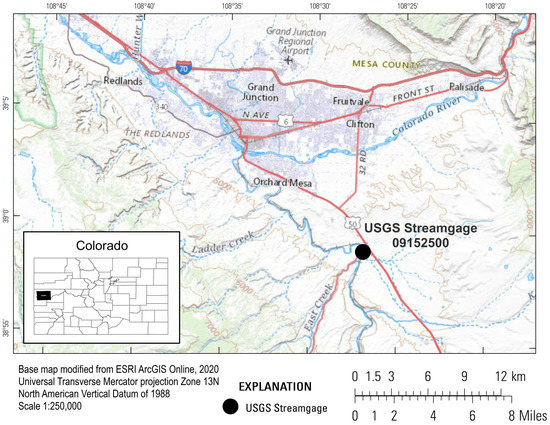
Figure 1.
Map of the study site collocated with USGS streamgage (09152500) on the Gunnison River near Grand Junction, Colorado. Elevations reported in meters above North American Vertical Datum (NAVD 88).
The Gunnison River is an armored, gravel-bed channel that drains an area of approximately 20,539 square kilometers (km2) at Whitewater Bridge [56,57,58]. The study site is located roughly 22 river-miles upstream from the confluence between the Gunnison River and the Colorado River at Grand Junction, Colorado, at an elevation of 1417 m (Figure 1), and the mean annual precipitation in the basin is 52 cm according to USGS StreamStats [56]. Runoff patterns in the region are dominated by the timing and magnitude of spring snowmelt; however, upstream reservoirs have altered the timing and magnitude of flood peaks on the Gunnison River since 1966 [59]. Consequently, peak flows have decreased substantially since 1966 [55,57,60]. The USGS streamgage (09152500) is located just upstream from the bridge and has measured daily discharge since 1896 [54]. Between 1919 (the first year when discharge data were published continuously) and 2019, the average (arithmetic mean) of the median, minimum, and maximum daily discharges were 43.3, 18.9, and 330.6 cubic meters per second (m3/s), respectively [54].
The Whitewater Bridge is a concrete, 5-span, rolled-I-Beam bridge, built in 1958, consisting of 4 sharp-nosed bridge piers that are 0.88 m wide [8]. The bridge is 9.75 m wide and 95.25 m in length [8]. At the time the POA was developed, the streambed under the bridge was composed of gravel and was underlain by a mixture of sand, gravel, boulders, and some finer particles (sand and silt) [8]. According to the CDOT POA for Whitewater Bridge, total pier scour depths associated with a 500-year flow event are estimated to be 3.14–4.21 m, which is a similar range to that of the magnitudes of estimated abutment scour depths (2.53–4.08 m) [8]. CDOT’s POA also identified thresholds for close monitoring or closure of the bridge based on stages that correspond to the 25-year and 50-year flow events, respectively [8].
2.2. Overview of Instrumentation and Data Collection
The experimental setup consisted of a single radar sensor (consisting of a Doppler velocity radar and pulsed stage radar) mounted to the Whitewater Bridge, a single-beam echosounder mounted to bridge pier 4 [8], and a traditional USGS streamgage located approximately 30 m upstream from the bridge (Figure 2). The radar was used to measure water surface velocity and stage, and to estimate discharge; the single-beam echosounder was used to measure streambed elevation at the bridge pier; and the pre-existing USGS streamgage provided validation for radar-based stage and discharge measurements. Data from the single-beam echosounder and USGS streamgage were collected during four snowmelt runoff seasons, and data from the radar were collected during one concurrent runoff season (Table 1).
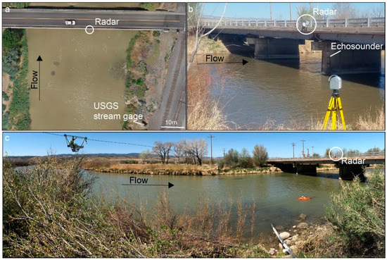
Figure 2.
Aerial photos of instrumentation with respect to the Whitewater Bridge taken by Mark Henneberg (a); side view of radar and single-beam echosounder mounted to the bridge (b); and panorama view of the cableway used to collect discharge measurements adjacent to the USGS streamgage and the Whitewater Bridge (c).

Table 1.
Overview of data collected, including instrumentation, measurements, and measurement time periods.
2.2.1. Single-Beam Echosounder Data Collection
One Airmar EchoRangeTM SmartTM Sensor echosounder (Airmar, Milford, NH, USA) was mounted on the east side of Whitewater Bridge pier 4, at the transition between the upstream nose and the straight section of the pier wall, to measure streambed elevation (Figure 2b). The echosounder was mounted at an elevation of 1412 m (as referenced to the National American Vertical Datum [NAVD] 88) and has a beam width of 9 degrees, which resulted in an acoustic footprint of about 0.36 m in diameter near the base of the pier (assuming a distance to streambed of about 3 m). The diameter of the acoustic footprint changed because of variations in streambed elevation over time. Streambed elevation data were recorded every 15 min and transmitted via satellite uplink every hour. Transmitted data are hosted on the National Water Information System (NWIS) database website for USGS streamgage 09152500 [54]. Sounding depths, which are traditionally collected to validate echosounder data, were not measured because during periods of high velocity (especially near the pier) conditions were not safe enough to access the area under the bridge monitored by the echosounder. Streambed elevation data collected by the single-beam echosounder were used for several purposes: changes in streambed elevation were used to compute event-based scour depths, and streambed elevation was subtracted from stage measurements to calculate flow depth at the bridge pier.
2.2.2. Radar Siting and Data Collection
Radar-based stage and velocity measurements were collected using an RQ-30 radar manufactured by Sommer Messtechnik, mounted to the Whitewater Bridge near pier 4 (Figure 2). The radar was sited directly above the y-axis (the axis representing stream depth), which is the location within a cross-section that contains the maximum depth-averaged velocity and maximum surface velocity [21,22,23,24,25,26,64,65], following the method described by [12]. The radar was sited and installed facing upstream to avoid complex streamflow patterns including eddies, secondary flows, and macroturbulence to the extent possible. Proper siting of the y-axis is necessary to estimate discharge using the PC method described in Section 2.3.1. See Figure 3 from [66] for an illustration of the y-axis defined from an acoustic Doppler current profiler (ADCP) profile.
The position of the y-axis was determined by first collecting a series of vertical velocity profiles along a cross-section immediately upstream from the bridge using an ADCP and a stationary moving bed test (SMBT). Velocity data from the SMBT was processed in WinRiver II software to determine the position of the y-axis and thus the location where the radar was installed. An R-script was then used to automatically extract parameters required for the PC method from the vertical velocity profile. Radar-based surface velocity and stage data were recorded every 15 min and transmitted every hour. Radar-based velocity, stage, and siting data were published by [61].
2.2.3. Conventional In-Stream Instrumentation and Measurements Used for Computations and Validation of Noncontact Data
Conventional methods were used to measure velocity, stage, and discharge to assist with siting the radar and assessing the accuracy of radar-based measurements. Cross-sectional channel geometry used to generate the stage–area rating for estimating radar-based discharge was measured using an ADCP at sections that were too deep to wade; these were measured using real-time kinematic global navigation satellite system along shallow sections and dry streambanks in accordance with protocols described by [67]. The cross-section was collected under the radar footprint and is published in [63]. Instantaneous or “site visit” measurements of velocity, stage, and discharge were made using in-stream mechanical current meters or ADCPs [68]. Site visit measurements were accessed using the dataRetrieval package in R [69,70].
Continuous estimates of river discharge at the USGS streamgage were empirically derived from stage–discharge curves based on the relation between river stage measurements collected with a bubbler system and discharge measurements collected during periodic site visits. All conventional measurements were collected in accordance with standard USGS protocols and accuracies [68,71]. Transmitted discharge and stage data are hosted on the NWIS website for USGS streamgage 09152500 or in USGS ScienceBase [54,62].
2.3. Data Analysis
2.3.1. Estimating Discharge from Radar Measurements Using the PC Method
Radar-based discharge was estimated using the PC method, an algorithm that can be used to estimate the mean channel velocity and discharge based on a coefficient, ϕ, defined as the ratio of mean velocity to maximum velocity. The PC method relies on a velocity distribution equation, pioneered by C.-L. Chiu [21,22,23,24,25,26,64,65], and based on Shannon’s Information Entropy [72]. Using the PC method, mean velocity is calculated as the product of ϕ and the maximum surface velocity measured by the radar at the y-axis. Radar-based discharge is computed as the product of ϕ, the maximum surface velocity, and the cross-sectional area (determined from a stage–area rating in stable boundary channels). Previous research indicates that ϕ remains constant during changes in stage, velocity, and discharge, assuming the stage–area relation remains constant [12,26]. Therefore, once established for a cross-section, ϕ can be used to compute a mean velocity and discharge for various flow conditions.
The radar-based surface velocity can be related to the Chiu velocity distribution, and subsequently to a mean channel velocity using Equations (1)–(5). Velocity distribution along the y-axis in probability space is represented by Equation (1):
In those instances when umax occurs at the water surface, the velocity distribution at the y-axis can be characterized by Equation (4):
The probability distribution f(u) is resilient (i.e., invariant with time and water level at a channel section) and, hence, its parameter M is constant at a channel section. h/D is a function of M and constant at a channel section [22].
The parameter ϕ, which is a function of M, can be computed using two methods: (1) using vertical velocity and depth data obtained from a single survey of the y-axis during radar siting; or (2) using multiple historical pairs of mean and maximum velocities obtained during site visits. The first option relies on data from ADCP surveys that can be measured and analyzed quickly, so that a ϕ value, and subsequently discharge estimates, can be computed from radar-based velocity measurements shortly after radar siting. With that method, values for umax, M(ϕ), and h/D are computed using a nonlinear estimator in R [73]. By default, Equations (2) and (4) are solved using a Gauss–Newton nonlinear least squares method. See Figures 4 and 5 from [66] for illustrations of observed and simulated vertical velocity profiles that coincide with the y-axis used to compute ϕ. In this study, ϕ estimates derived from the first method, based on a single survey of the y-axis, are referred to as “rapid” ϕ estimates.
The second method relies on concurrent mean and maximum velocity measurements, where mean velocity is derived from a conventional discharge measurement; the greater the number of paired measurements and range of velocities, the more robust the ϕ estimate [12,22,74]. Although the second method is preferred, it requires additional time and site visits. In this study, ϕ estimates derived from the second method are referred to as “trained” ϕ estimates.
The coefficient ϕ is defined for both the “rapid” ϕ and “trained” ϕ methods in Equation (5):
Once ϕ has been calculated, radar-based discharge is calculated based on umax, which can be measured in real time (e.g., [12]), and Equation (6):
where Q = discharge and A = cross-sectional area.
In this study, radar-based discharge was computed in two ways. First, radar-based discharge was computed using the PC method parameterized with the “rapid-ϕ” value, derived from a vertical velocity profile collected at the y-axis at the time of installation, estimates of cross-sectional area derived from radar-based stage, previously collected cross-section profiles, and estimates of the maximum surface velocity measured by the radar. Radar-based discharge resulting from this first method is henceforth referred to as the fully radar-based discharge.
To assess the extent to which radar-based discharge estimates would be improved by a more robust ϕ value and more stable stage measurements, discharge was also computed using the PC method parameterized with the “trained-ϕ” value, derived from multiple USGS site visits during the time the radar was operating, estimates of cross-sectional area derived from USGS-streamgage-based stage, and estimates of the maximum surface velocity measured by the radar. The trained-ϕ value was calculated from 15 measurements of cross-sectionally averaged velocity, measured during USGS site visits, and maximum surface velocity, measured by the radar. Discharges during the 15 USGS site visits ranged from 21 to 405 m3/s. Radar-based discharge resulting from the second method is henceforth referred to as the hybrid-radar-based approach. A locally weighted smoothing (LOESS) filter was applied to both hybrid and fully radar-based datasets to eliminate spikes using the loess function in R, assuming a second-order polynomial and span (which controls the degree of smoothing) of 0.007 [69]; both the unfiltered (raw) and LOESS-filtered datasets are evaluated in the results section.
Radar-based discharge estimates derived from additional combinations of stage and ϕ values were also computed and are published in Appendix A for reference. Those combinations included fully radar-based discharge estimates calculated using the trained-ϕ value and hybrid-radar-based discharge estimates calculated using the rapid-ϕ value.
2.3.2. Statistical Metrics Used to Assess Radar-Based Measurement Accuracy
The accuracies of radar-based stage and discharge measurements were evaluated against conventional, streamgage-based measurements made at the collocated USGS streamgage for the time period when both sets of measurements overlapped (February 2019–August 2019). A series of quantitative statistics—including the root mean square error (RMSE), mean absolute error (MAE), percent bias (PBIAS), Pearson correlation coefficient (r), Nash–Sutcliffe efficiency (NSE) coefficient, Kling–Gupta efficiency (KGE) coefficient, alpha (αKGE), and, in the case of discharge, volumetric efficiency (VE)—were used to measure the goodness of fit between the radar-based (simulated) and the USGS-streamgage-based measurements (observed) using the HydroGOF package in R [75]. Statistical metrics were used to evaluate the goodness of fit for the full dataset and for the 1st, 2nd, 3rd, and 4th quartiles of the dataset to assess whether the agreement between the radar-based and the USGS-streamgage-based measurements varied with flow magnitude.
Both RMSE and MAE were used to quantify the average errors between radar-based and USGS-streamgage-based measurements, in units of the variables of interest. MAE measures the average magnitude of the absolute value of errors, and therefore weighs all errors equally, without consideration of direction [76,77]. RMSE measures the square root of the mean square error and weights larger errors more heavily [76,77,78]. Both MAE and RMSE vary from 0 to ∞, with 0 indicating perfect agreement between simulated and observed values. RMSE and MAE values less than half the standard deviation are considered to be low [79], which was the same criteria adopted in this study to represent satisfactory agreement between radar-based and streamgage-based measurements.
PBIAS measures the average tendency of simulated data to be larger or smaller than observed data [77]. A PBIAS value of 0.0 is optimal; positive PBIAS values indicate the simulated data underestimate observed data; and negative PBIAS values indicate the simulated data overestimate observed data [77,80]. Generally, model performance is considered very good when PBIAS falls between −10% and 10% and is considered good when PBIAS falls between 10% and 15% or −10% and −15% [77]. In this study, PBIAS values falling between −15% and 15% were considered satisfactory. The Pearson correlation coefficient (r) represents the degree of collinearity between simulated and observed data and varies between −1, for perfect negative correlation, and 1, for perfect positive correlation [76,77]. Although the criteria for satisfactory model performance based on r values is not well established in the literature (e.g., [77,81]), r values > 0.90 were considered satisfactory in this study.
The Nash–Sutcliffe efficiency coefficient (NSE) is another metric used to assess the level of agreement between radar-based and streamgage-based measurements. The NSE coefficient is a measure of the magnitude of error variance in the simulated data normalized by the magnitude of error variance in observed data [82]. The NSE coefficient is a normalized measure of agreement between simulated and observed values that ranges from −∞ to 1 [82]. An NSE value greater than 0 indicates that simulated values are as accurate as the mean of the observed data, and an NSE value of 1 indicates a perfect match between the two datasets. Generally, an NSE value greater than 0.75 indicates very good agreement between simulated and observed data [77,83], and NSE values greater than 0.75 were considered satisfactory in this study.
Although NSE is a normalized metric, it has been shown to overemphasize differences at large flows due to the squaring of deviations [76,84]. A complementary metric for comparing simulated and observed discharge data is volumetric efficiency (VE) [78]. VE weights all disparities between simulated and observed data equally. VE represents the fraction of water delivered with correct timing and varies from 0 to 1 [78]. Although the criteria for satisfactory model performance based on VE values are not well established in the literature (e.g., [77,81]), VE values > 0.85 were considered satisfactory in this study, which is a more conservative threshold compared with an NSE of 0.75 [78].
Lastly, the original KGE (another alternative to the NSE) and one of KGE’s components, αKGE (a measure of the flow variability error), were used to assess agreement between radar-based and streamgage-based measurements [85,86,87,88]. KGE is composed of the same statistical elements as NSE, but is a reformulation designed to correct underestimation of discharge variability [85,86,89]. KGE ranges from −∞ to 1, and a value of −0.41 indicates simulated values are as accurate as the mean of the observed data (in comparison, an NSE = 0 corresponds to the mean flow benchmark) [88]. The parameters used to calculate KGE include the following: r—the Pearson correlation coefficient; β—the ratio between simulated and observed means; and αKGE—the ratio between simulated and observed standard deviations [85,86,89]. Ideal values of r, β, and αKGE are 1 [85,86,88,89]. Although the criteria for satisfactory model performance based on KGE and αKGE values is not well established in the literature (e.g., [77,81]), in this study, KGE values greater than 0.75, and αKGE values between 0.85 and 1.15, were considered satisfactory.
2.3.3. Estimating Scour Depth Based on Time-Integrated Stream Power per Unit Area (Ω) and the Onset of Sediment Motion
Time-integrated stream power per unit area, Ω (in joules), also referred to as energy per unit area in the literature, was defined as:
where t is the time in seconds, and ω is unit stream power (in W/m2), defined as:
where is water density in kg/m3, g is gravitational acceleration in m/s2, Q is discharge in m3/s, S is the water surface slope in m/m, and B is water surface width in meters [32,33,34,45]. Note that the definition of Ω in this study is consistent with [45,47]; however, others have defined Ω differently as the total stream power equal to (in units of W/m) (e.g., [34]). To calculate ω, Q was derived from both continuous USGS streamgage records collected over the 4-year monitoring period and from (LOESS-filtered) radar-based measurements collected during the last year of monitoring. Slope (S) was estimated from an empirical relation between Q and S measured by [90]. Channel top width (B) was estimated from stage measurements and the stage–width curve, derived from cross-sectional geometry measured at the bridge.
The Ω values were calculated for periods when sustained flows exceeded the critical threshold for sediment motion at the bridge pier. On the rising and falling limbs of the snowmelt hydrograph, flow occasionally oscillated above and below the threshold for sediment motion. For the purposes of calculating Ω, the beginning of an event was defined as the time when flow first exceeded the threshold for sediment motion after a period of low flow lasting at least 2 weeks; the end of an event was defined as the time when flow exceeded the threshold for sediment motion, prior to a period of low flow lasting at least 2 weeks. Over the course of an entire high-flow event, there were brief periods (less than 2 weeks in duration) when flow did not exceed the threshold for sediment transport, which, by definition, were not included in the calculation for Ω.
Periods when flow exceeded the threshold for sediment motion at the bridge pier were defined by times when the ratio of shields stress to critical shields stress () exceeded unity. Shields stress () is defined as:
where H is the flow depth at the bridge pier in m, is the density of quartz sediment in kg/m3, and is the median grain size based on Wolman pebble counts [91] of surface particles, conducted by [90] on active gravel bars located within 250 ft upstream or downstream from the USGS streamgage. We assume that the onset of sediment motion can reasonably be determined based on the because differences in particle exposure offset differences in particle size [92,93,94,95,96,97].
Although the streambed material at the bridge pier was not sampled directly, the approach presented in this study is intended to be representative of an inexpensive but less precise method for characterizing sediment size when compared with more comprehensive evaluations of scour depth, such as the ones found in POAs. Consequently, we assume that the sampled streambed material is representative of the material that composes the streambed at the pier and the material that fills the scour hole. However, we acknowledge that material sourced from the scour hole at depth or supplied from upstream may be different from the material sampled on gravel bars used to characterize the in this study, which is a limitation of this study.
In order to discern whether the results of this study were sensitive to variations in , critical shields stress () was estimated from two separate empirical equations based on the slope (S) [97,98]. The values calculated using the equation by [97], based on empirical data from flumes and natural streams, are henceforth referred to as . The values calculated using the equation by [98], based on measurements of flow and bedload transport from 45 gravel-bed rivers in Northwestern America, are referred to as .
Flow depth at the bridge pier was estimated by subtracting the streambed elevation measured by the single-beam echosounder from water stage (elevation) measured by either the radar or the USGS streamgage. The raw streambed elevation data measured by the single-beam echosounder was noisy, so a LOESS curve, fit to the raw streambed elevation data, was used in calculations of flow depth. Streambed elevation data were only available during periods when the water surface elevation was high enough to submerge the echosounder, which was mounted above the streambed to avoid debris. As a result, streambed elevation data were missing during periods when the stage was low, which typically occurred between snowmelt-driven peak discharges.
The maximum event scour depth was defined as the maximum difference between the streambed elevation at the beginning of the high-flow event, when the ratio exceeded unity for the first time, and the minimum streambed elevation at the time of scour. Streambed elevation at the beginning of the high-flow event was calculated as the average of streambed elevation values, measured over the 24 h preceding the time at which the ratio exceeded unity for the first time. The minimum streambed elevation at the time of scour was defined as the minimum recorded elevation following the largest recorded monotonic decrease in streambed elevation and preceding a period of stable streambed elevation or increased streambed elevation. Nondimensional scour depth, or relative scour depth, was calculated by dividing the maximum event scour depth (ys) by pier width (b). The Ω value associated with the minimum streambed elevation (maximum relative scour depth) was recorded as the value hypothesized to scale with ys/b.
3. Results
Scour was detected during all three high-flow events that exceeded the critical threshold for sediment motion ( > 1). High-flow events peaked in May or June 2016, 2017, and 2019, and were numbered sequentially for reference (i.e., high-flow events 1, 2, and 3, respectively). The magnitude of peak discharges associated with high-flow events 1–3 ranged from 297 to 486 m3/s, and their recurrence intervals were 1.7, 4.2, and 4.7 years, respectively (Table 2 and Figure 3). Recurrence intervals were calculated using the USGS software program PeakFQ version 7.2 [99] and the same method as [100], based on annual peak discharge measurements between 1897 and 2019. Flow depths measured at the bridge pier during peak discharges ranged from 4.99 to 5.64 m, and the maximum surface velocity measured during the peak discharge of high-flow event 3, the only event for which surface velocity was measured, was 2.92 m/s (Table 2). Streambed elevation data were recorded during the majority of high-flow events 1, 2, and 3, when the single-beam echosounder was submerged, and were also recorded during the prolonged low-flow period that occurred in 2018. During the 2018 low-flow period, streambed elevations and corresponding stage were higher compared with previous low-flow periods.
Table 2.
Timing and flow characteristics of the peak discharges recorded during high-flow events 1–3.
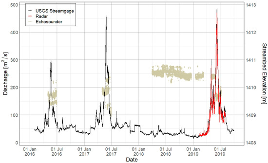
Figure 3.
Time series of discharge and streambed elevation datasets collected at the study site. The black line represents discharge estimates generated from conventional methods at the USGS streamgage (09125000), the red line denotes discharge estimates generated from the PC method based on measurements from the radar, and the tan circles denote streambed elevation data collected from the single-beam echosounder. Discharge estimates are in cubic meters per second and correspond with the primary (left-hand) y-axis, whereas streambed elevation data are in meters above NAVD 88 and correspond with the secondary (right-hand) y-axis.
3.1. Performance of Radar-Based Stage and Discharge Estimates
3.1.1. Overview of Radar-Based Measurement Performance
The accuracies of radar-based stage and discharge measurements were evaluated against conventional, streamgage-based measurements made at the collocated USGS streamgage for the time period when both sets of measurements overlapped during high-flow event 3 (February 2019–August 2019). Overall, the agreement between radar-based and USGS-streamgage-based estimates of stage and discharge was good, and all goodness-of-fit statistics for the entire datasets (all time periods and quartiles) exceeded criteria for satisfactory performance. In general, radar-based measurements captured the timing of acute changes in flow conditions, but overpredicted stage measurements and underpredicted USGS-streamgage-based discharge measurements at higher flows.
3.1.2. Radar-Based Stage Performance
Statistical metrics based on the entire dataset (all quartiles) and individual quartiles (1st–4th) indicated very good agreement between radar-based stage and streamgage-based stage measurements and exceeded this study’s criteria for satisfactory performance as outlined in Section 2.3.2 (Table 3, Figure 4). However, radar-based stage measurements were larger and more variable than streamgage-based measurements, particularly at higher stages (Table 3, Figure 4). For example, MAE and RMSE values associated with the upper two quartiles of stage data were larger compared with values associated with the lower two quartiles, indicating that deviations between radar-based and streamgage-based stage measurements were larger (in absolute terms) at higher stage (Table 3). Although PBIAS values for all quartiles were zero, indicating no detectable bias in radar-based stage estimates, αKGE values associated with the upper two quartiles of stage data exceeded 1, indicating that radar-based stage estimates were more variable than streamgage-based measurements at higher stages.
Table 3.
Goodness-of-fit statistics associated with radar-based and USGS-streamgage-based stage measurements, values in bold indicate they meet this study’s criteria for satisfactory performance defined in Section 2.3.2.
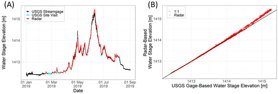
Figure 4.
Comparisons of radar-based stage data (red), continuous USGS-streamgage-based stage data (black), and USGS site visit stage data (cyan), that include (A) a time series of all datasets and (B) a scatterplot of radar-based stage data vs. USGS continuous streamgage-based data. Elevation data are in meters above NAVD 88.
3.1.3. Radar-Based Discharge Performance
Statistical metrics indicated that overall agreement between both sets of radar-based discharge estimates and USGS-streamgage-based discharge estimates was good, and that fully radar-based discharge estimates underperformed hybrid-radar-based discharge estimates (Table 4 and Figure 5). Following the workflow outlined in Section 2.3.1, the rapid-ϕ value used to calculate fully radar-based discharge estimates was 0.52, and the trained-ϕ value used to calculate hybrid-radar-based discharge estimates was 0.58. All statistical metrics based on both radar-based datasets exceeded this study’s definition of satisfactory performance; although, some metrics associated with the 1st, 2nd, and 3rd quartiles did not (Table 4). For both sets of radar-based discharge estimates, metrics associated with the upper two quartiles of discharge data, when sediment was estimated to be mobile, outperformed metrics from the lower two quartiles, when sediment was estimated to be immobile.
Table 4.
Goodness-of-fit statistics associated with radar-based and USGS-streamgage-based discharge measurements, values in bold indicate they meet this study’s criteria for satisfactory performance defined in Section 2.3.2. (a) contains statistics from the fully radar-based, rapid-ϕ dataset in the format unfiltered (raw) data/LOESS-filtered data, and (b) contains statistics from the hybrid-radar-based, trained-ϕ dataset in the format unfiltered (raw) data/LOESS-filtered data.
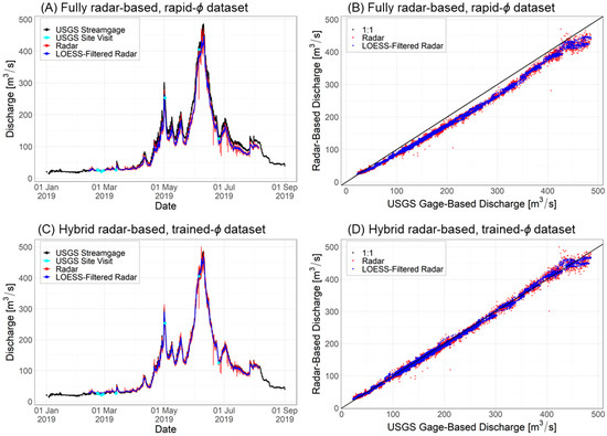
Figure 5.
Comparisons of unfiltered (raw) radar-based discharge estimates (red), LOESS-filtered radar-based discharge estimates (royal blue), continuous USGS-streamgage-based discharge estimates (black), and USGS site visit stage discharge measurements (cyan), for the fully radar-based, rapid-ϕ dataset (A,B) and the hybrid-radar-based, trained-ϕ dataset (C,D). These include the time series of both datasets (A,C) and scatterplots of both radar-based discharge datasets versus USGS continuous streamgage-based datasets (B,D).
Both the fully and hybrid-radar-based discharge estimates were generally effective at capturing discharge magnitude and the timing of acute changes in discharge (Figure 5). For both radar-based datasets, the improved agreement between the LOESS-filtered discharge estimates and the streamgage-based discharge estimates can be seen graphically; the LOESS-filtered data are less noisy compared with unfiltered (raw) data (Figure 5). In addition, LOESS filtering reduced spikes in discharge, which marginally improved statistical agreement between radar-based and streamgage-based discharges (Table 4).
Although fully radar-based discharge estimates adequately captured the timing and volume of flows (all VE values were >0.85 and KGE values exceeded 0.75, with the exception of the 1st quartile), they underpredicted streamgage-based discharges at all flow magnitudes (overall PBIAS of about 12%) (Table 4, part (a); and Figure 5). The MAE, RMSE, and PBIAS values associated with the fully radar-based dataset were at least triple the values associated with the hybrid-radar-based dataset (with the exception of the 1st quartile), indicating comparatively poorer performance. The NSE, VE, KGE, and αKGE values derived from fully radar-based discharge estimates were also lower than values derived from hybrid-radar-based discharge estimates, indicating poorer overall performance in terms of magnitude, timing, and variability. Despite the poorer performance of fully radar-based discharge estimates, NSE, VE, KGE, and αKGE values still met the criteria for satisfactory performance defined in this study (with the exception of the 1st quartile) (Table 4, part (a)). The underprediction of streamgage-based discharge estimates was attributed to underestimation of the rapid-ϕ value, which was substantial enough to offset inflation in fully radar-based discharge estimates caused by overpredictions in radar-based stage (Figure 4).
Hybrid-radar-based discharge estimates (both unfiltered (raw) and LOESS-filtered discharge estimates) outperformed fully radar-based discharge estimates, with the exception of data within first quartile (Table 4). Overall, data derived from the hybrid-radar-based approach were characterized by very low MAE, RMSE, and PBIAS statistics, and near-perfect NSE, VE, KGE, αKGE, and r values (Table 4, part (b)). Such favorable metrics indicate that hybrid-radar-based discharge estimates matched USGS-streamgage-based discharge estimates almost perfectly in terms of flow magnitude, timing, and variability. Hybrid-radar-based discharge estimates within the 2nd through 4th quartiles slightly overestimated streamgage-based estimates (PBIAS between 1.03 and 2.54%), whereas discharge estimates within the 1st quartile were not satisfactory and overpredicted streamgage-based discharge by over 10% (Table 4). Despite those minor discrepancies, at 0.97, the VE for the entire dataset was nearly perfect for both unfiltered and LOESS-filtered datasets (Table 4, part (b)). These metrics, along with time series and 1:1 plots, allow for visual comparison between the radar-based and streamgage-based discharge estimates, and confirm that the hybrid-radar-based approach performed very well (Table 4 and Figure 5).
3.2. Observations on Bridge Pier Scour and Ω
Bridge pier scour was detected during all three high-flow events that exceeded the critical threshold for sediment transport and occurred on the rising limb of each event (Figure 6). The minimum streambed elevation at the time of scour, used to calculate the maximum scour depth, was interpreted from timeseries of streambed elevation (Figure 6). The minimum streambed elevations during high-flow events 1 and 3 (black arrows within Figure 6) were straightforward to identify because those minimums followed monotonic declines in streambed elevation and preceded periods of stable or increasing streambed elevation. Streambed elevation data were noisier and less straightforward to interpret during high-flow event 2 (Figure 6). During high-flow event 2, we interpreted the minimum streambed elevation to correspond with the smallest recorded streambed elevation on the rising limb (Figure 6).
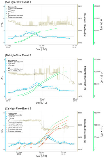
Figure 6.
Time series of shields stress ratios (, blue tones), Ω values (green tones for data based on USGS streamgage measurements and orange tones for data based on radar-derived measurements), streambed elevation (tan points), and LOESS-filtered streambed elevation values (brown line) for individual high-flow events 1 (A), 2 (B), and 3 (C). Vertical black arrows correspond to the minimum streambed elevation at the time of scour.
Accumulated debris may have obfuscated the streambed underneath the echosounder and led to noisier and elevated streambed elevation measurements during high-flow event 2, which may explain why streambed elevation data were difficult to interpret. An alternative or additional explanation for noisy streambed elevation measurements is that the location of the scour hole may have shifted relative to the position of the echosounder. Three observations lend confidence to our interpretation of the minimum streambed elevation during high-flow event 2: (1) the scour event occurred on the rising limb of the hydrograph, which is consistent with conventional knowledge on the timing of pier scour under live-bed conditions [32]; (2) the streambed elevation data measured around the time of scour were consistent over a continuous 1 h period; and (3) the streambed elevation at the time of scour were consistent with more reliable streambed elevation values recorded over the falling limb and after flow fell below the threshold for sediment motion, which supports the interpretation that debris may have obfuscated the streambed. Ultimately, however, the time of scour during high-flow event 2 is not definitive, and we acknowledge that the lack of a clearly defined minimum streambed elevation and our inability to collect soundings to validate the echosounder data are a weakness of this study. Results from high-flow event 2 also illustrate the challenges associated with using and interpreting echosounder data.
Based on measurements of scour depth and Ω, high-flow event 1 (in 2016) was characterized by the smallest scour depth and smallest Ω value at the time of scour; high-flow event 2 (in 2017) was characterized by the second-largest scour depth and Ω value at the time of scour; and high-flow event 3 (in 2019) was characterized by the largest scour depth and Ω value at the time of scour (Table 5). For each high-flow event, estimates of Ω varied depending on which value was used to determine when sediment was mobile (either or ). Total flow durations and Ω values were both larger when calculated using values because they corresponded to lower sediment transport thresholds compared with values (Table 5 and Figure 6). Consequently, flows that were close to on the rising and falling limbs of the hydrograph often exceeded but not . At the end of high-flow events 1, 2, and 3, Ω values calculated using were 1.5, 1.2, and 1.7 times greater, respectively, compared with Ω values calculated using (based on data from Table 5).
Table 5.
Stream power and scour measurement results (including relative scour depth (scour depth [ys] normalized by pier width [b], or ys/b) for each high-flow event, discharge estimation method, and value. “NA” refers to data that are not applicable.
Additionally, Ω estimates varied depending upon the discharge estimate (either radar-based or streamgage-based) used in calculations. Results indicated that Ω values calculated using the hybrid-radar-based discharge estimates were slightly less (PBIAS 0.78–1.24%) than Ω values calculated using USGS-streamgage-based discharge estimates, whereas Ω values calculated using fully radar-based discharge estimates were much less (PBIAS 11.12–32.70%) than Ω values calculated using USGS-streamgage-based discharge estimates (Table 6). Those findings were consistent with results from Section 3.1.2, which showed better agreement between hybrid-radar-based discharge estimates and streamgage-based discharge estimates than between fully radar-based discharge estimates and streamgage-based discharge estimates (Table 4 and Table 6). Despite differences between radar-based and streamgage-based Ω values, the hybrid-radar-based results and fully radar-based results calculated using still exceeded this study’s criteria for satisfactory performance, although fully radar-based results calculated using did not (Table 6).
Table 6.
Goodness-of-fit statistics associated with radar-based and USGS-streamgage-based Ω estimates in the following format: derived/ derived. Values in bold indicate they meet this study’s criteria for satisfactory performance defined in Section 2.3.2.
3.3. Comparison of Observed Scour Depth and Simulated Scour Depth Based on Pier Scour Equations
Although evaluating the accuracy of existing pier scour equations was not the focus of this study, here we present a brief comparison of observed and predicted scour depths. Scour depths were estimated from three commonly used pier scour equations, including the Hydraulic Engineering Circular 18 (HEC-18) pier scour equation (based on the Colorado State University equation) reported by [32] (Equation (7.1)), the updated HEC-18 pier scour equation for non-cohesive soils reported by [101] (Equation (19)), and the pier scour equation developed for Colorado mountain streams by [53] (Equation (18)). Scour depths were simulated for high-flow event 3, which was the only high-flow event with available velocity data (Table 2 and Figure 3). The maximum surface velocity recorded by the radar was transformed to the depth-averaged approach velocity using an α coefficient of 0.8 ([102,103]). Relative scour depths (scour depth [ys] normalized by pier width [b], or ys/b) estimated using the methods due to [32], [101], and [53] were 2.16 m/m, 2.05 m/m, and 1.18 m/m, respectively, which all exceeded the measured ys/b of 0.98 m/m. Relative scour depth (ys/b) simulated using the [53] method was closest to the measured ys/b.
3.4. Relation between Relative Scour Depth (ys/b) and Time-Integrated Stream Power per Unit Area (Ω)
Relative scour depth (ys/b) was positively correlated with the magnitude of Ω at the time of scour (Table 5, Figure 7). Exponential trendlines were fit to data derived from USGS streamgage data based on and to illustrate the range of conditions represented by the data and the predictive capabilities of this approach using the nls function from the stats package in R [69]. Pearson correlation coefficients (r) values ranged from 0.94 to 0.99, indicating strong correlations (Figure 7). For equivalent Ω values, trendlines based on USGS streamgage data underpredicted ys/b values associated with radar-based data, particularly the fully radar-based data points. Underprediction of ys/b values associated with radar-based data was attributed to underestimation bias in radar-based discharge estimates and thus Ω estimates.

Figure 7.
Relative scour depth (ys/b) as a function of Ω for different datasets. Exponential trendline equations and Pearson correlation coefficients (r) associated with USGS streamgage data based on and are shown in dark green and light green, respectively.
Although data from additional scour events would be needed to verify the robustness of the trendlines presented in Figure 7, observations on the evolution of ys/b with increasing Ω can be made. For example, the shape of the trendline indicates that ys/b increases more rapidly at larger Ω values and increases more slowly at smaller Ω values (Figure 7). The upper portion of the curve (ys/b > 1), however, is poorly constrained and is likely inaccurate. The maximum ys/b ratio observed in natural systems or physical experiments is 3.6 depending on Froude number and pier shape [31,32,104,105]. According to [31], the maximum observable ys/b in natural systems is 2.5. However, if one were to extrapolate the trendline presented in Figure 7 to ys/b = 2 (which is still well below the maximum limit of ys/b), therefore doubling of the maximum ys/b observed in this study, then the result would correspond to an unrealistically large Ω value, associated with an event larger than the Bonneville paleoflood [45,106] (Figure 7). Ultimately, additional data would be needed to test the robustness of the trendline and to constrain its trajectory at larger values of ys/b.
4. Discussion
4.1. Utility of Radars for Monitoring the Hydraulic Conditions That Contribute to Bridge Pier Scour
In this study, we demonstrated that radars can be used to monitor the hydraulic conditions (stage and discharge) that contribute to bridge pier scour. In comparison with USGS streamgage data, radar-based measurements captured the timing and magnitude of discharge and stage satisfactorily, especially during higher flows when larger quantities of bed sediment were mobile and the potential for deep scour was greatest [52]. Our findings are also consistent with results from a study by [12], which found close agreement between radar-based and USGS-streamgage-based discharges at 10 different sites over a range of flow conditions.
In addition to providing information on the magnitude and timing of flow events that could be critical in information-poor areas, radars have several other advantages. First, radars can be used to produce usable stage and discharge estimates within a day of installation. The only information needed to begin estimating discharge using radar-based measurements and the PC method is a cross-sectional profile, to generate a stage–area rating, and a vertical velocity profile at the y-axis, to estimate a rapid-ϕ value. In comparison, discharge estimates generated from traditional streamgages may be more accurate, but those estimates are generated from stage–discharge rating curves that require many site visits and potentially many months to establish [107]. Consequently, compared with traditional streamgages, radars may provide real-time discharge measurements much more quickly and more cheaply; although, these benefits might be partially offset by losses in data quality.
Additionally, radars are mounted above flowing water and debris and are therefore less susceptible to damage. As a result, they may be characterized by lower maintenance costs compared with in-stream monitoring instruments such as sonar or sounding rods for bridge scour monitoring [1], or pressure transducer and stilling well instruments for stage/discharge monitoring. For example, in this study, two single-beam echosounders were initially installed for redundancy, but one was damaged during a high-flow event and consequently excluded from analyses. Radars can also be mounted directly to a bridge, close to telemetry and power supply, which reduces the need for costly infrastructure. Lastly, radars are safer to operate compared with in-stream instrumentation because they can be installed and serviced outside of the wetted channel.
Noncontact, radar-based measurements (i.e., stage, surface velocity, and discharge) could be incorporated into scour monitoring plans in several ways. One approach for estimating scour depth based on Ω values derived from radar measurements was presented in this study. Real-time stage, surface velocity, and discharge measurements could also be used to trigger scour alerts predefined in a POA [1]. At Whitewater Bridge, for example, in-person monitoring is triggered by an exceedance of the discharge or stage corresponding to 820 m3/s (25-year flow event) at the collocated USGS streamgage [8]. Closure of the bridge is triggered by an exceedance of the discharge or stage corresponding to 975 m3/s (50-year flow event) [8]. In the absence of data from a pre-existing streamgage, stage or discharge measurements from radars could be used to trigger scour monitoring alerts, such as the ones defined in POAs; although, more information on the accuracy of radar-based measurements under varying environmental conditions would be needed before relying on them for safety interventions.
Although the noncontact monitoring approach presented in this study provided good-quality data and improved upon several limitations of traditional methods, the accuracies of noncontact measurements were influenced by several factors unique to radars that merit further consideration, including the number of site visit measurements used to constrain the ϕ-value, proper radar siting, and the measurement of unobstructed flow (e.g., outside the influence of bridge piers). The factor that played the largest role in improving the accuracy of radar-based discharge estimates was using a trained-ϕ value instead of a rapid-ϕ value, even though that modification would also require more intensive data collection. The trained-ϕ value substantially improved discharge estimates by reducing the PBIAS value from about 12%, based on fully radar-based discharge measurements, to only about 1%, based on hybrid-radar-based discharge estimates. Although determining an ideal or a minimum number of site visit measurements to estimate a trained-ϕ value was beyond the scope of this study, collecting measurements across a wide range of flows is more important than collecting a large number of measurements to constrain the trained-ϕ value [12].
Additionally, proper radar siting is key to collecting accurate stage, and thus discharge, estimates [12]. In this study, radar-based stage measurements were consistently larger than USGS-streamgage-based stage measurements, particularly at higher flows. Differences in stage may be explained by differences in the hydraulic conditions encountered by the USGS streamgage and the bridge-mounted radar. The USGS streamgage was located approximately 30 m upstream from the Whitewater Bridge, along a free-flowing section of the river, whereas the radar was mounted to the bridge itself, facing upstream. Deviations in stage estimates were likely caused by “backwater rise”, which refers to an increase in water surface elevation just upstream from bridge piers caused by a reduction in the cross-sectional area of the flow and is a phenomenon amplified at greater discharges [108]. Radar-based stage measurements could therefore be improved by installing the radar in a location that does not experience flow pileup at higher stages but does experience the same hydraulic conditions (i.e., water stage and discharge) measured by the USGS streamgage.
In terms of the physical siting of the radar, mounting the radar away from the piers—either on the bridge deck in between piers or outward on a boom to avoid the pier’s sphere of influence—may improve measurement agreement. If the ideal site for measuring radar-based stage is not coincident with the y-axis, where radar-based velocity is measured, then two separate radars could be installed at different locations within the cross-section to optimize data quality. However, installing two separate stage and velocity radars would likely add additional cost and complexity to the radar–gage design.
Wind and secondary flows, which added noisiness to stage and velocity measurements, are additional factors that warrant consideration (and need to be minimized) to the extent possible during site selection. Wind can bias measurements in both positive and negative directions depending on its direction; although, if wind measurements are available, then they can be used to correct biases and reduce noise in radar-based discharge estimates [12]. Secondary flows, such as eddies, that persist at the water surface for periods similar to or longer than the radar sampling duration (used to determine the dominant velocity), can also cause additional noise and spikes in surface velocity measurements [12]. Depending on the setting, noisiness due to wind and secondary flows can be improved by increasing the velocity sampling duration, so long as the duration remains shorter than the rate at which stage and velocity are changing. Alternatively, LOESS filtering could be incorporated directly into data collection platforms to eliminate noise and spikes. Although LOESS filtering did not improve agreement between radar-based and streamgage-based data substantially (it only marginally improved goodness-of-fit statistics (Table 3 and Table 4)), eliminating noise and spikes could be important for preventing false alerts in a scour monitoring capacity.
Disparities between radar-based and streamgage-based stage and discharge caused by siting, wind, and other factors have several implications for scour monitoring. Radar-based stage was consistently greater than USGS-streamgage-based stage, which could cause stage-related monitoring thresholds to be exceeded prematurely. Conversely, fully radar-based discharge was consistently lower than USGS-streamgage-based discharge, which could cause discharge-related monitoring thresholds to be exceeded too late for adequate warning. However, data quality, and thus the accuracy of scour alert triggers, could be improved by implementing the aforementioned operational changes. Overall, the good statistical agreement between radar-based and USGS-streamgage-based flow measurements indicates that radars are a viable option for scour monitoring.
4.2. Applicability of Ω for Estimating Relative Scour Depth (ys/b)
Based on a limited dataset collected over three high-flow events, Ω values at the time of scour were found to be strongly correlated with ys/b, indicating that Ω values can be used to estimate scour depth. A positive correlation between Ω values and ys/b was expected because numerous previous studies have shown that stream power is related to the processes that control scour. For example, stream power is correlated with channel-shaping processes that include sediment transport [34,35,36,37,38], channel aggradation and degradation [39], morphodynamics [40,41,42,43,44], geomorphic change [45,46,47,48], landscape incision rates [109,110], and sediment grain size selection [49]. A precedence also exists for using cumulative stream power in scour monitoring because it scales with the depth of erosion into bedrock or cohesive soils in the absence of alluvial cover [27,28,29,30,32,33,111]. Although the mechanics of erosion into bedrock are different from erosion in alluvial channels, cumulative stream power scales with underlying drivers of erosion common to both processes (i.e., flow magnitude and duration). Therefore, under transport limited conditions, the results of this study support the premise that Ω can be used to estimate scour depth.
In addition, the Ω metric better reflects both the magnitude and duration of flow and characterizes the flow conditions and flow history that contribute to scour compared with traditional methods. Scour depth is not instantaneous and instead depends on both flow magnitude and the length of time a given flow is sustained and exceeds the threshold for sediment transport, which is not captured, for example, in traditional bridge scour equations based on the magnitude of instantaneous flow metrics, such as velocity or depth [32,112]. In some ways, the results of this study echo the conceptual model put forth by [45], who posited that the degree of landscape modification (or in this case, scour) resulting from a flow event depends upon both the intensity and duration of flow that exceeds resistance thresholds, quantified by Ω, and not solely upon the extent to which an event exceeds resistance thresholds (quantified by flow magnitude).
The quantitative relation between Ω and ys/b defined in this study can be leveraged to model pier scour depth for several applications. The principal advantage of the Ω-based approach is that it models scour depth along a defined trajectory, which enables a user to assess and even predict scour depth in real time, in response to changes in flow and streambed elevation (i.e., changes in Ω). The shape of the relation between Ω and ys/b may also play a role in the urgency of heightened monitoring when observed Ω values correspond to critical scour depths that may pose a risk to the structural integrity of the bridge. For example, more vigilant monitoring may be needed during periods when ys/b values rise sharply with increases in Ω (Figure 7), assuming those periods coincide with, or immediately precede, critical levels of ys/b. Although simulating ys/b in real time based on Ω values may not serve as the primary line of defense in assessing scour risk, it may provide complementary information to an existing scour monitoring plan, which would be helpful in the event that an in situ sensor was damaged by high water or debris.
Another advantage of the Ω-based approach is that ys/b can be simulated under a range of different flow scenarios (represented by variations in Ω) to identify the set of flow conditions that minimize or maximize scour. Depending on the site, results from a scour sensitivity analysis could provide guidance on the timing, magnitude, and duration of streamflow that minimizes scour depth. Conversely, streamflow patterns that lead to ys/b values associated with critical scour risk could also be identified. If sufficient historical data were available, those flow conditions could be compared against the historical flow record to examine the frequency of scour critical events and the environmental conditions that generated them (e.g., precipitation intensity, snowpack levels). However, as noted in the results section, the relation between Ω and ys/b presented in this study was poorly constrained and likely inaccurate at values of ys/b > 1, limiting its present utility for examining large scour events.
Despite its advantages for monitoring scour risk in real time, the Ω-based approach presented in this study has several limitations. First, the simulated relation between Ω and ys/b presented in this study is an empirical correlation between flow energy and relative scour depth [113], not a direct measure of the physical processes that cause pier scour, which include flow-acceleration- and current-induced vortices [32,114,115]. Consequently, previously collected discharge and scour depth data would be needed to build the relation between Ω and ys/b, and the strength of the correlation between those two variables is only as reliable as the quality of the input data. In this study, for example, differences in the ways discharge was computed using the PC method, and differences in values of used to compute Ω, led to some variability in the relation between Ω and ys/b (Figure 7). A large source of variability in Ω estimates was the choice of value, so if could be determined more precisely, perhaps empirically [95], then the uncertainty would be reduced. Alternatively, a range of values (such as +/−25%) could be computed to test the sensitivity of Ω, however Ω values would still be dependent on the chosen value.
Another challenge with building an empirical relation between Ω and ys/b is the time required to collect the input data needed to build the relation. Although the data derived from radar measurements (i.e., discharge and Ω) can be collected very quickly after the instrument is installed, ys/b values from a minimum of three unique scour events are still needed. In this study, ys/b data took 4 years to collect, which may be prohibitively long depending on monitoring timelines. Ideally, more than three data points that span a wide range of ys/b values would be used to build a robust relation. Good data quality is also needed to build a reliable empirical relation between Ω and ys/b; however, as was the case with high-flow event 2, data quality can be reduced by debris or other factors. In lieu of reliable data, the time needed to build an empirical relation between Ω and ys/b may be lengthened. A long data-collection period could be circumvented if historical scour and discharge data were available at the site; although, such circumstances are rare.
In addition to the challenges associated with building an empirical relation between Ω and ys/b, the second limiting feature of the Ω-based approach is that without more data from Whitewater Bridge or other study sites, the simulated trendline presented in this study is not transferrable to other sites. Although it may be possible to apply the relation between Ω and ys/b simulated in this study to similar armored gravel-bed rivers, there is no previous work to support that idea. Nondimensional metrics similar to Ω, such as the total flow work index that scales with bedload yield [116,117,118] or the effective flow work that scales with scour depth and rate [119,120], may be related to ys/b across rivers of different sizes; however, those metrics cannot be tested without discharge and scour data from additional sites. So, although it was beyond the scope of this study to examine the degree to which Ω is correlated with ys/b at other sites, with additional data, it may be possible to do so. A widely applicable relation between Ω, or similar dimensionless metrics, and ys/b would be especially powerful because it would eliminate the need to collect discharge and scour depth data in advance and, combined with radars, would make the implementation of the Ω-based approach very fast (operational within days of installation).
The third limitation of the Ω-based approach is that it is not entirely noncontact because it relies upon measurements of streambed elevation collected with a single-beam echosounder. Streambed elevation measurements were used to estimate ys/b and local flow depth at the bridge pier. The latter was used to calculate and determine when flow conditions exceeded the threshold for sediment transport (and thus when Ω > 0). Several strategies could be adopted to make the Ω-based approach entirely noncontact. For example, noncontact instruments capable of measuring scour and streambed elevation directly, such as ground-penetrating radar or continuous seismic reflection profiling, could be used instead of a single-beam echosounder; although, those instruments are not yet fully operational for scour monitoring applications [1,11,13,14,15,16,17,18,19]. Alternatively, could be estimated from surface velocity measurements rather than from flow depth using the entropy theory [65], although that method relies on von Karman’s constant, which studies have shown is nonuniversal in flows with low submergence or during sediment transport [121]. Another strategy that may be suitable at certain sites, and would eliminate the need for real-time flow depth measurements, would be to impose a static streambed elevation and assume that changes in flow depth due to fluctuations in streambed elevation are small in comparison with the total flow depth. However, that strategy would introduce additional errors and underestimate discharge, , and ultimately Ω. An alternative strategy would be to determine the threshold for sediment transport from critical ω values derived from discharge estimates rather than from values derived from flow depth measurements [27,28,122,123]. However, without taking into account real-time scour and increases in the cross-sectional area, that method would also lead to underestimates of discharge and Ω.
The fourth limitation of the Ω-based approach is that it does not account for sediment supply. Under high sediment supply conditions, for example, scour depths would be overestimated using the Ω-based approach if the rate of sediment in-filling exceeded the rate of sediment removal within the scour hole [32,124]. However, that same limitation also applies to most other methods for estimating bridge pier scour [32,52,124,125]. Lastly, the Ω-based approach provides a coarse estimate of scour depth and, as a result, does not account for differences in the strength of flow acceleration and deceleration on the rising and falling limbs of the hydrograph that may influence scour [119,126,127,128].
Despite these limitations, Ω values provide a reasonable estimate of scour depth and therefore represent one strategy for utilizing radar-based data that could supplement existing scour monitoring plans and provide useable data quickly in remote, previously ungaged locations—albeit with potentially lower accuracy than more intensive scour monitoring or modeling techniques.
5. Conclusions
This study presents a straightforward framework for using noncontact methods to measure the stage and streamflow conditions that contribute to bridge pier scour, as well as a method for using those measurements to estimate bridge pier scour depth in real time based on discharge-derived Ω values. Results indicated there was good agreement between radar-based and USGS-streamgage-based stage and discharge estimates on the Gunnison River, Colorado; although, radar-based estimates of discharge underpredicted USGS-streamgage-based estimates of discharge, particularly at high flows. Additionally, using a trained-ϕ value instead of a rapid-ϕ value substantially improved the accuracy of radar-based discharge estimates, but required more intensive field data collection. Overall, the good statistical agreement between radar-based and USGS-streamgage-based stage and discharge measurements indicates that radars are viable tools for measuring the hydraulic conditions that contribute to bridge pier scour.
Another key finding was that Ω values at the time of scour were strongly correlated with ys/b, indicating that Ω values derived from radar measurements can be used to coarsely estimate scour potential when paired with limited field measurements (i.e., slope, cross-sectional geometry, and surface grain size). The principal advantage of the Ω-based approach is that the relation between Ω and ys/b could be leveraged to assess and even predict scour potential in real time in response to changes in flow and streambed elevation; although, more work would be helpful to verify the robustness of the relation between Ω and ys/b before implementing the approach in an operational setting.
The Ω-based approach also has several limitations that effect its transferability and feasibility: (1) additional data would be needed to verify whether the site-specific relation between Ω and ys/b could be replicated at other critical scour sites on gravel-bed rivers; (2) good-quality data from at least three scour events would be needed to build a relation between Ω and ys/b, which could take several years to collect; (3) the method is not entirely noncontact because it relies on streambed elevation data to measure flow depth, which is used to estimate when the threshold for sediment transport is exceeded; and (4) the approach does not account for changes in sediment supply. Despite those limitations, utilizing radar-derived Ω estimates to assess bridge pier scour potential is a promising approach designed to be implemented quickly and cost effectively. The approach is not intended to replace the existing high-fidelity scour monitoring techniques, but rather to supplement existing scour monitoring techniques and to provide coarse and less expensive data quickly in information-poor areas.
Author Contributions
Conceptualization, J.W.F. and M.F.H.; methodology, J.W.F. and M.F.H.; software, L.A.H., H.F.M., J.W.F. and J.R.C.; validation, all authors; formal analysis, L.A.H. and H.F.M.; investigation, all authors; resources, J.W.F. and M.F.H.; writing—original draft preparation, L.A.H. and H.F.M.; writing—review and editing, all authors; visualization, L.A.H. and H.F.M.; supervision, J.W.F.; project administration, J.W.F.; funding acquisition, J.W.F. and H.F.M. All authors have read and agreed to the published version of the manuscript.
Funding
This research was supported by the Colorado Department of Transportation and the U.S. Geological Survey.
Data Availability Statement
Data availability are summarized in Table 1. USGS streamgage data (stage, discharge, and streambed elevation from the echosounder) are published in NWIS at https://waterdata.usgs.gov/co/nwis/uv?site_no=09152500 (accessed on 1 March 2022) [54] or in ScienceBase at https://doi.org/10.5066/P98283OI (accessed on 1 March 2022) [62]. Radar stage and velocity can be accessed at https://doi.org/10.5066/P98DC3DX (accessed on 1 March 2022) [61]. The cross-section profile can be accessed at https://doi.org/10.5066/P92EY47R (accessed on 1 March 2022) [63].
Acknowledgments
The authors would like to recognize Mike Kohn (USGS) for his support in the field. Any use of trade, firm, or product names is for descriptive purposes only and does not imply endorsement by the U.S. Government.
Conflicts of Interest
The authors declare no conflict of interest, and the funders had no role in the design of the study; in the collection, analyses, or interpretation of data; in the writing of the manuscript, or in the decision to publish the results.
Appendix A
Figure A1.
Comparisons of unfiltered (raw) radar-based discharge estimates (red), LOESS-filtered radar-based discharge estimates (royal blue), continuous USGS-streamgage-based discharge estimates (black), and USGS site visit stage discharge measurements (cyan), for the fully radar-based, trained-ϕ dataset, including a time series (left) and a scatterplot (right).
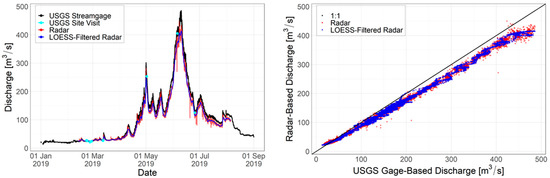
Figure A2.
Comparisons of unfiltered (raw) radar-based discharge estimates (red), LOESS-filtered radar-based discharge estimates (royal blue), continuous USGS-streamgage-based discharge estimates (black), and USGS site visit stage discharge measurements (cyan), for the hybrid-radar-based, rapid-ϕ dataset, including a time series (left) and a scatterplot (right).

Table A1.
Goodness-of-fit statistics associated with radar-based and USGS-streamgage-based discharge measurements, from the fully radar-based, trained-ϕ dataset. Values in bold indicate they meet this study’s criteria for satisfactory performance defined in Section 2.3.2.
Table A1.
Goodness-of-fit statistics associated with radar-based and USGS-streamgage-based discharge measurements, from the fully radar-based, trained-ϕ dataset. Values in bold indicate they meet this study’s criteria for satisfactory performance defined in Section 2.3.2.
| Parameter | Entire Dataset | 1st Quartile | 2nd Quartile | 3rd Quartile | 4th Quartile |
|---|---|---|---|---|---|
| Mean absolute error (MAE), in m3/s | 5.66/5.69 | 2.78/2.78 | 3.90/4.24 | 6.23/6.16 | 9.67/9.51 |
| Root mean square error (RMSE), in m3/s | 7.44/7.73 | 3.06/3.15 | 4.65/4.89 | 7.24/6.81 | 11.72/12.59 |
| Percent bias (PBIAS), in percentage | 1.68/1.67 | −9.98/−9.86 | 4.89/5.33 | 4.42/4.45 | 0.57/0.40 |
| Nash–Sutcliffe Efficiency (NSE), dimensionless | 0.99/0.99 | −0.02/−0.07 | 0.97/0.97 | 0.81/0.83 | 0.98/0.98 |
| Volumetric efficiency (VE), dimensionless | 0.96/0.95 | 0.90/0.90 | 0.95/0.94 | 0.95/0.95 | 0.96/0.96 |
| Kling–Gupta efficiency (KGE), dimensionless | 0.98/0.98 | 0.66/0.70 | 0.93/0.92 | 0.95/0.95 | 0.90/0.90 |
| Alpha (αKGE), dimensionless | 1.01/1.01 | 0.69/0.75 | 0.96/0.94 | 1.01/0.99 | 1.10/1.10 |
| Pearson correlation coefficient (r), dimensionless | 1.00/1.00 | 0.93/0.86 | 1.00/1.00 | 0.97/0.98 | 1.00/1.00 |
Table A2.
Goodness-of-fit statistics associated with radar-based and USGS-streamgage-based discharge measurements, from the hybrid-radar-based, rapid-ϕ dataset. Values in bold indicate they meet this study’s criteria for satisfactory performance defined in Section 2.3.2.
Table A2.
Goodness-of-fit statistics associated with radar-based and USGS-streamgage-based discharge measurements, from the hybrid-radar-based, rapid-ϕ dataset. Values in bold indicate they meet this study’s criteria for satisfactory performance defined in Section 2.3.2.
| Parameter | Entire Dataset | 1st Quartile | 2nd Quartile | 3rd Quartile | 4th Quartile |
|---|---|---|---|---|---|
| Mean absolute error (MAE), in m3/s | 14.37/14.34 | 1.27/1.16 | 9.45/9.00 | 16.73/16.70 | 29.93/30.41 |
| Root mean square error (RMSE), in m3/s | 18.91/19.13 | 1.62/1.43 | 10.40/10.02 | 17.17/17.50 | 32.01/32.45 |
| Percent bias (PBIAS), in percentage | 11.11/11.11 | −0.38/−0.51 | 12.62/12.04 | 12.32/12.30 | 11.26/11.45 |
| Nash–Sutcliffe efficiency (NSE), dimensionless | 0.97/0.96 | 0.72/0.78 | 0.86/0.87 | −0.07/−0.11 | 0.88/0.88 |
| Volumetric efficiency (VE), dimensionless | 0.96/0.89 | 0.90/0.96 | 0.95/0.88 | 0.95/0.88 | 0.96/0.89 |
| Kling–Gupta efficiency (KGE), dimensionless | 0.84/0.84 | 0.69/0.65 | 0.82/0.83 | 0.84/0.86 | 0.86/0.86 |
| Alpha (αKGE), dimensionless | 0.89/0.88 | 0.72/0.66 | 0.87/0.89 | 0.90/0.95 | 0.91/0.91 |
| Pearson correlation coefficient (r), dimensionless | 1.00/1.00 | 0.86/0.92 | 1.00/0.99 | 0.98/0.95 | 1.00/1.00 |
References
- Lagasse, P.F.; Clopper, P.E.; Pagan-Ortiz, J.E.; Zevenbergen, L.W.; Arneson, L.A.; Schall, J.D.; Girard, L.G. Bridge Scour and Stream Instability Countermeasures: Experience, Selection, and Design Guidance-Third Edition; No. FHWA-NHI-09-111; U.S. Department of Transportation Federal Highway Administration: Vienna, VA, USA, 2009; Volume 2.
- Murrillo, J.A. The Scourge of Scour. Civ. Eng. ASCE 1987, 57, 66–69. [Google Scholar]
- Butch, G.K. Measurement of Bridge Scour at Selected Sites in New York, Excluding Long Island; Report 91-4083; US Geological Survey Water Resources Investigations: Reston, VA, USA, 1991.
- Wardhana, K.; Hadipriono, F.C. Analysis of Recent Bridge Failures in the United States. J. Perform. Constr. Facil. 2003, 17, 144–150. [Google Scholar] [CrossRef] [Green Version]
- Rhodes, J.; Trent, R. Economics of Floods, Scour and Bridge Failures. In Hydraulic Engineering; ASCE: Reston, VA, USA, 1993. [Google Scholar]
- Deng, L.; Cai, C.S. Bridge Scour: Prediction, Modeling, Monitoring and Countermeasures—Review. Pract. Period. Struct. Des. Constr. 2010, 15, 125–134. [Google Scholar] [CrossRef] [Green Version]
- Briaud, J.-L.; Hurlebaus, S.; Chang, K.-A.; Yao, C.; Sharma, H.; Yu, O.-Y.; Darby, C.; Hunt, B.E.; Price, G.R. Realtime Monitoring of Bridge Scour Using Remote Monitoring Technology; Texas Transportation Institute: Bryan, TX, USA, 2011. [Google Scholar]
- Colorado Department of Transportation. Drainage Report for Structure I–03–A State Highway 141 over the over the Gunnison River; Colorado Department of Transportation: Denver, CO, USA, 2012.
- Prendergast, L.J.; Gavin, K. A Review of Bridge Scour Monitoring Techniques. J. Rock Mech. Geotech. Eng. 2014, 6, 138–149. [Google Scholar] [CrossRef]
- Corato, G.; Moramarco, T.; Tucciarelli, T. Continuous Discharge Monitoring Using Non-Contact Methods for Velocity Measurements: Uncertainty Analysis. In Engineering Geology for Society and Territory; Springer: Cham, Switzerland, 2015; Volume 3. [Google Scholar]
- Hong, S.; Wiggenhauser, H.; Helmerich, R.; Dong, B.; Dong, P.; Xing, F. Long-Term Monitoring of Reinforcement Corrosion in Concrete Using Ground Penetrating Radar. Corros. Sci. 2017, 114, 123–132. [Google Scholar] [CrossRef]
- Fulton, J.W.; Mason, C.A.; Eggleston, J.R.; Nicotra, M.J.; Chiu, C.L.; Henneberg, M.F.; Best, H.R.; Cederberg, J.R.; Holnbeck, S.R.; Lotspeich, R.R.; et al. Near-Field Remote Sensing of Surface Velocity and River Discharge Using Radars and the Probability Concept at 10 U.S. Geological Survey Streamgages. Remote Sens. 2020, 12, 1296. [Google Scholar] [CrossRef] [Green Version]
- Placzek, G.; Haeni, F.P. Surface-Geophysical Techniques Used to Detect Existing and Infilled Scour Holes near Bridge Piers. In Water-Resources Investigations Report 95-4009; US Geological Survey: Reston, VA, USA, 1995. [Google Scholar]
- Haeni, F.P. Use of Ground-Penetrating Radar and Continuous Seismic-Reflection Profiling on Surface-Water Bodies in Environmental and Engineering Studies. J. Environ. Eng. Geophys. 1996, 1, 27–35. [Google Scholar] [CrossRef]
- Spicer, K.R.; Costa, J.E.; Placzek, G. Measuring Flood Discharge in Unstable Stream Channels Using Ground-Penetrating Radar. Geology 1997, 25, 423–426. [Google Scholar] [CrossRef]
- Costa, J.E.; Spicer, K.R.; Cheng, R.T.; Haeni, F.P.; Melcher, N.B.; Thurman, E.M.; Plant, W.J.; Keller, W.C. Measuring Stream Discharge by Non-Contact Methods: A Proof-of-Concept Experiment. Geophys. Res. Lett. 2000, 27, 553–556. [Google Scholar] [CrossRef]
- Haeni, F.P.; Buursink, M.L.; Costa, J.E.; Melcher, N.B.; Cheng, R.T.; Plant, W.J. Ground Penetrating Radar Methods Used in Surface-Water Discharge Measurements. In Proceedings of the 8th International Conference on Ground Penetrating Radar, Gold Coast, Australia, 23–26 May 2000; SPIE: Bellingham, WA, USA, 2000; Volume 4084. [Google Scholar]
- Melcher, N.B.; Costa, J.E.; Haeni, F.P.; Cheng, R.T.; Thurman, E.M.; Buursink, M.; Spicer, K.R.; Hayes, E.; Plant, W.J.; Keller, W.C.; et al. River Discharge Measurements by Using Helicopter-Mounted Radar. Geophys. Res. Lett. 2002, 29, 2084. [Google Scholar] [CrossRef] [Green Version]
- Anderson, N.L.; Ismael, A.M.; Thitimakorn, T. Ground-Penetrating Radar: A Tool for Monitoring Bridge Scour. Environ. Eng. Geosci. 2007, 13, 1–10. [Google Scholar] [CrossRef]
- Fulton, J.W.; Anderson, I.E.; Chiu, C.L.; Sommer, W.; Adams, J.D.; Moramarco, T.; Bjerklie, D.M.; Fulford, J.M.; Sloan, J.L.; Best, H.R.; et al. QCam: SUAS-Based Doppler Radar for Measuring River Discharge. Remote Sens. 2020, 12, 3317. [Google Scholar] [CrossRef]
- Chiu, C. Velocity Distribution in Open Channel Flow. J. Hydraul. Eng. 1989, 115, 576–594. [Google Scholar] [CrossRef]
- Chiu, C. Entropy and Probability Concepts in Hydraulics. J. Hydraul. Eng. 1987, 113, 589–599. [Google Scholar] [CrossRef]
- Moramarco, T.; Saltalippi, C.; Singh, V.P. Estimation of Mean Velocity in Natural Channels Based on Chiu’s Velocity Distribution Equation. J. Hydrol. Eng. 2004, 9, 42–50. [Google Scholar] [CrossRef]
- Chiu, C.L.; Hsu, S.M. Probabilistic Approach to Modeling of Velocity Distributions in Fluid Flows. J. Hydrol. 2006, 316, 28–42. [Google Scholar] [CrossRef]
- Chiu, C.-L.; Tung, N.-C. Maximum Velocity and Regularities in Open-Channel Flow. J. Hydraul. Eng. 2002, 128, 390–398. [Google Scholar] [CrossRef]
- Chiu, C.L.; Hsu, S.M.; Tung, N.C. Efficient Methods of Discharge Measurements in Rivers and Streams Based on the Probability Concept. Hydrol. Process. 2005, 19, 3935–3946. [Google Scholar] [CrossRef]
- Annandale, G.W. Erodabilité. J. Hydraul. Res. 1995, 33, 471–494. [Google Scholar] [CrossRef]
- Annandale, G.; Smith, S. Calculation of Bridge Pier Scour Using the Erodibility Index Method; Colorado Department of Transportation Report No. CDOT-DTD-R-2000-9; Golder Associates: Lakewood, CO, USA, 2001.
- Dickenson, S.E.; Baillie, M.W. Predicting Scour in Weak Rock of the Oregon Coast Range; Final Report SPR 382; Oregon Department of Transportation Research Group: Salem, OR, USA, 1999.
- Armitage, N.; McGahey, C.; Rooseboom, A.; Abt, S.R.; Johnson, T.L.; Thornton, C.I.; Trabant, S.C.; Buffington, J.M.; Abban, B.; Paphitis, D.; et al. A Unit Stream Power Model for the Prediction of Local Scour in Rivers. J. Hydraul. Eng. 2007, 140, 1098. [Google Scholar]
- Ettema, R.; Constantinescu, G.; Melville, B. Evaluation of Bridge Scour Research: Pier Scour Processes and Predictions; Transportation Research Board of the National Academies: Washington, DC, USA, 2011. [Google Scholar]
- Arneson, L.A.; Zevenbergen, L.W.; Lagasse, P.F.; Clopper, P.E. Evaluating Scour at Bridges, 5th ed.; Report FHWA-HIF-12-003; U.S. Department of Transportation Federal Highway Administration: Vienna, VA, USA, 2012.
- Keaton, J.R.; Mishra, S.K.; Clopper, P.E. Scour at Bridge Foundations on Rock; The National Academies Press: Washington, DC, USA, 2012; Volume 717. [Google Scholar] [CrossRef]
- Bagnold, R. Sediment Discharge and Stream Power—A Preliminary Announcement; Circular 421; US Geological Survey: Reston, VA, USA, 1960.
- Bagnold, R.A. An Approach to the Sediment Transport Problem from General Physics; Professional Paper 422-I; US Geological Survey: Washington, DC, USA, 1966.
- Yang, C.T. Unit Stream Power and Sediment Transport. J. Hydraul. Div. 1972, 98, 1805–1826. [Google Scholar] [CrossRef]
- Yang, C.T.; Stall, J.B. Unit Stream Power for Sediment Transport in Natural Rivers; Illinois State Water Survey: Champaign, IL, USA, 1974. [Google Scholar]
- Yang, C.T.; Molinas, A. Sediment Transport and Unit Stream Power Function. J. Hydraul. Div. 1982, 108, 774–793. [Google Scholar] [CrossRef]
- Bull, W.B. Threshold of Critical Power in Streams. Bull. Geol. Soc. Am. 1979, 90, 453–464. [Google Scholar] [CrossRef]
- Nanson, G.C.; Hickin, E.J. A Statistical Analysis of Bank Erosion and Channel Migration in Western Canada. Geol. Soc. Am. Bull. 1986, 97, 497–504. [Google Scholar] [CrossRef]
- Nanson, G.C.; Croke, J.C. A Genetic Classification of Floodplains. Geomorphology 1992, 4, 459–486. [Google Scholar] [CrossRef] [Green Version]
- McEwen, L.J. Channel Planform Adjustment and Stream Power Variations on the Middle River Coe, Western Grampian Highlands, Scotland. Catena 1994, 21, 357–374. [Google Scholar] [CrossRef]
- Larsen, E.W.; Fremier, A.K.; Greco, S.E. Cumulative Effective Stream Power and Bank Erosion on the Sacramento River, California, USA. J. Am. Water Resour. Assoc. 2006, 42, 1077–1097. [Google Scholar] [CrossRef]
- Bizzi, S.; Lerner, D.N. The Use of Stream Power as an Indicator of Channel Sensitivity to Erosion and Deposition Processes. River Res. Appl. 2015, 31, 16–27. [Google Scholar] [CrossRef]
- Costa, J.E.; O’Connor, J.E. Geomorphically Effective Floods; Cost, J.E., Miller, A.J., Potter, A.W., Wilcock, P.R., Eds.; Geophysical Monograph 90; American Geophysical Union: Washington, DC, USA, 1995; Volume 89. [Google Scholar]
- Buraas, E.M.; Renshaw, C.E.; Magilligan, F.J.; Dade, W.B. Impact of Reach Geometry on Stream Channel Sensitivity to Extreme Floods. Earth Surf. Process. Landf. 2014, 39, 1778–1789. [Google Scholar] [CrossRef]
- Magilligan, F.J.; Buraas, E.M.; Renshaw, C.E. The Efficacy of Stream Power and Flow Duration on Geomorphic Responses to Catastrophic Flooding. Geomorphology 2014, 228, 175–188. [Google Scholar] [CrossRef]
- Yochum, S.E.; Sholtes, J.S.; Scott, J.A.; Bledsoe, B.P. Stream Power Framework for Predicting Geomorphic Change: The 2013 Colorado Front Range Flood. Geomorphology 2017, 292, 178–192. [Google Scholar] [CrossRef]
- Snyder, N.P.; Nesheim, A.O.; Wilkins, B.C.; Edmonds, D.A. Predicting Grain Size in Gravel-Bedded Rivers Using Digital Elevation Models: Application to Three Maine Watersheds. Bull. Geol. Soc. Am. 2013, 125, 148–163. [Google Scholar] [CrossRef] [Green Version]
- Chase, K.J.; Holnbeck, S.R. Evaluation of Pier-Scour Equations for Coarse-Bed Streams; Report 2004-5111; US Geological Survey Scientific Investigations: Reston, VA, USA, 2004.
- Toth, E.; Brandimarte, L. Prediction of Local Scour Depth at Bridge Piers under Clear-Water and Live-Bed Conditions: Comparison of Literature Formulae and Artificial Neural Networks. J. Hydroinform. 2011, 13, 812–824. [Google Scholar] [CrossRef] [Green Version]
- Brandimarte, L.; Paron, P.; di Baldassarre, G. Bridge Pier Scour: A Review of Processes, Measurements and Estimates. Environ. Eng. Manag. J. 2012, 11, 975–989. [Google Scholar] [CrossRef]
- Molinas, A.; Mommandi, A.; Khan, A.; Sollenberger, B. Developing Bridge-Scour Equations for Colorado Mountain Streams CDOT-2018-10; Department of Transportation: Washington, DC, USA, 2018.
- US Geological Survey. US Geological Survey National Water Information System Database. In USGS Water Data for the Nation; US Geological Survey: Reston, VA, USA, 2020. [Google Scholar] [CrossRef]
- Henneberg, M.F. Real-Time Streambed Scour Monitoring at Two Bridges over the Gunnison River in Western Colorado, 2016–2017; US Geological Survey: Reston, VA, USA, 2018.
- USGS The StreamStats Program. 2019. Available online: http://water.usgs.gov/osw/streamstats/colorado.html (accessed on 10 May 2020).
- Pitlick, J.; van Steeter, M.; Barkett, B.; Cress, R.; Franseen, M. Geomorphology and Hydrology of the Colorado and Gunnison Rivers and Implications for Habitats Used by Endangered Fishes; US Fish and Wildlife Service: Washington, DC, USA, 1999.
- Pitlick, J.; Mueller, E.R.; Segura, C.; Cress, R.; Torizzo, M. Relation between Flow, Surface-Layer Armoring and Sediment Transport in Gravel-Bed Rivers. Earth Surf. Process. Landf. 2008, 33, 1192–1209. [Google Scholar] [CrossRef]
- Dubinski, I.M.; Wohl, E. Assessment of Coarse Sediment Mobility in the Black Canyon of the Gunnison River, Colorado. Environ. Manag. 2007, 40, 147–160. [Google Scholar] [CrossRef] [PubMed]
- Elliot, J.G.; Hammack, L.A. Geomorphic and Sedimentologic Characteristics of Alluvial Reaches in the Black Canyon of the Gunnison National Monument, Colorado; Report 99-4082; US Geological Survey Water-Resources Investigations: Reston, VA, USA, 1999.
- Fulton, J.W.; McDermott, W.R.; Mason, C.A. Radar-Based Field Measurements of Surface Velocity and Discharge from 10 U.S. Geological Survey Streamgages for Various Locations in the United States, 2002–2019; US Geological Survey Data Release: Denver, CO, USA, 2020. [CrossRef]
- Henneberg, M.F.; Hempel, L.A. Gage Height Data from February through September for Years 2016–19 at Gunnison River near Grand Junction, Colorado; US Geological Survey Data Release: Denver, CO, USA, 2022. [CrossRef]
- Henneberg, M.F. Cross-Section Geometry at Two Bridges over the Gunnison River in Western Colorado; US Geological Survey Data Release: Denver, CO, USA, 2018. [CrossRef]
- Chiu, C.; Chiou, J. Structure of 3D Flow in Rectangular Open Channels. J. Hydraul. Eng. 1986, 112, 1050–1067. [Google Scholar] [CrossRef]
- Moramarco, T.; Dingman, S.L. On the Theoretical Velocity Distribution and Flow Resistance in Natural Channels. J. Hydrol. 2017, 555, 777–785. [Google Scholar] [CrossRef]
- Fulton, J.; Ostrowski, J. Measuring Real-Time Streamflow Using Emerging Technologies: Radar, Hydroacoustics and the Probability Concept. J. Hydrol. 2008, 357, 1–10. [Google Scholar] [CrossRef]
- Rydlund, P.H.; Densmore, B.K. Methods of Practice and Guidelines for Using Survey-Grade Global Navigation Satellite Systems (GNSS) to Establish Vertical Datum in the United States Geological Survey; Book 11; US Geological Survey Techniques and Methods: Reston, VA, USA, 2012.
- Mueller, D.S.; Wagner, C.R. Measuring Discharge with Acoustic Doppler Current Profilers from a Moving Boat. In U.S. Geological Survey Techniques and Methods 3-A22; US Geological Survey: Reston, VA, USA, 2009. [Google Scholar]
- RC. Team. R Core Team R: A Language and Environment for Statistical Computing. In R Foundation for Statistical Computing; R Core Team: Vienna, Austria, 2019. [Google Scholar]
- De Cicco, L.A.; Lorenz, D.; Hirsch, R.M.; Watkins, W.; Johnson, M. DataRetrieval: R Packages for Discovering and Retrieving Water Data Available from U.S. Federal Hydrologic Web Services; US Geological Survey: Reston, VA, USA, 2020.
- Turnipseed, D.P.; Sauer, V.B. Discharge Measurements at Gaging Stations: U.S. Geological Survey Techniques and Methods Book 3; US Geological Survey: Reston, VA, USA, 2010.
- Shannon, C.E. A Mathematical Theory of Communication. Bell Syst. Tech. J. 1948, 27, 379–423. [Google Scholar] [CrossRef] [Green Version]
- Gonzalez, J.A.; Melching, C.S.; Oberg, K.A. Analysis of Open-Channel Velocity Measurements Collected with an Acoustic Doppler Current Profiler. In Proceedings of the 1st International Conference on New/Emerging Concepts for Rivers, Chicago, IL, USA, 22–25 September 1996; IWR Association: Chicago, IL, USA, 1996. [Google Scholar]
- Costa, J.E.; Cheng, R.T.; Haeni, F.P.; Melcher, N.; Spicer, K.R.; Hayes, E.; Plant, W.; Hayes, K.; Teague, C.; Barrick, D. Use of Radars to Monitor Stream Discharge by Noncontact Methods. Water Resour. Res. 2006, 42, W07422. [Google Scholar] [CrossRef]
- Zambrano, M.B. Package “HydroGOF”: Goodness-of-Fit Functions for Comparison of Simulated and Observed Hydrological Time Series; R Package Version 4.0. 2020. Available online: https://github.com/hzambran/hydroGOF (accessed on 1 March 2022).
- Legates, D.R.; McCabe, G.J. Evaluating the Use of “goodness-of-Fit” Measures in Hydrologic and Hydroclimatic Model Validation. Water Resour. Res. 1999, 35, 233–241. [Google Scholar] [CrossRef]
- Moriasi, D.N.; Arnold, J.G.; van Liew, M.W.; Bingner, R.L.; Harmel, R.D.; Veith, T.L. Model Evaluation Guidelines for Systematic Quantification of Accuracy in Watershed Simulations. Trans. ASABE 2007, 50, 885–900. [Google Scholar] [CrossRef]
- Criss, R.E.; Winston, W.E. Do Nash Values Have Value? Discussion and Alternate Proposals. Hydrol. Process. 2008, 22, 2723–2725. [Google Scholar] [CrossRef]
- Singh, J.; Knapp, H.V.; Arnold, J.G.; Demissie, M. Hydrological Modeling of the Iroquois River Watershed Using HSPF and SWAT. J. Am. Water Resour. Assoc. 2005, 41, 343–360. [Google Scholar] [CrossRef]
- Gupta, H.V.; Sorooshian, S.; Yapo, P.O. Status of Automatic Calibration for Hydrologic Models: Comparison with Multilevel Expert Calibration. J. Hydrol. Eng. 1999, 4, 135–143. [Google Scholar] [CrossRef]
- Bennett, N.D.; Croke, B.F.W.; Guariso, G.; Guillaume, J.H.A.; Hamilton, S.H.; Jakeman, A.J.; Marsili-Libelli, S.; Newham, L.T.H.; Norton, J.P.; Perrin, C.; et al. Characterising Performance of Environmental Models. Environ. Model. Softw. 2013, 40, 1–20. [Google Scholar] [CrossRef]
- Nash, J.E.; Sutcliffe, J.V. River Flow Forecasting through Conceptual Models Part I—A Discussion of Principles. J. Hydrol. 1970, 10, 282–290. [Google Scholar] [CrossRef]
- Schaefli, B.; Gupta, H.V. Do Nash Values Have Value? Hydrol. Process. 2007, 21, 2075–2080. [Google Scholar] [CrossRef] [Green Version]
- Krause, P.; Boyle, D.P.; Bäse, F. Comparison of Different Efficiency Criteria for Hydrological Model Assessment. Adv. Geosci. 2005, 5, 89–97. [Google Scholar] [CrossRef] [Green Version]
- Gupta, H.V.; Kling, H.; Yilmaz, K.K.; Martinez, G.F. Decomposition of the Mean Squared Error and NSE Performance Criteria: Implications for Improving Hydrological Modelling. J. Hydrol. 2009, 377, 80–91. [Google Scholar] [CrossRef] [Green Version]
- Kling, H.; Fuchs, M.; Paulin, M. Runoff Conditions in the Upper Danube Basin under an Ensemble of Climate Change Scenarios. J. Hydrol. 2012, 424, 264–277. [Google Scholar] [CrossRef]
- Thirel, G.; Andréassian, V.; Perrin, C.; Audouy, J.-N.; Berthet, L.; Edwards, P.; Folton, N.; Furusho, C.; Kuentz, A.; Lerat, J.; et al. Hydrology under Change: An Evaluation Protocol to Investigate How Hydrological Models Deal with Changing Catchments. Hydrol. Sci. J. 2015, 60, 1184–1199. [Google Scholar] [CrossRef]
- Knoben, W.J.M.; Freer, J.E.; Woods, R.A. Technical Note: Inherent Benchmark or Not? Comparing Nash-Sutcliffe and Kling-Gupta Efficiency Scores. Hydrol. Earth Syst. Sci. 2019, 23, 4323–4331. [Google Scholar] [CrossRef] [Green Version]
- Santos, L.; Thirel, G.; Perrin, C. Technical Note: Pitfalls in Using Log-Transformed Flows within the KGE Criterion. Hydrol. Earth Syst. Sci. 2018, 22, 4583–4591. [Google Scholar] [CrossRef] [Green Version]
- Williams, C.A.; Schaffrath, K.R.; Elliott, J.G.; Richards, R.J. Application of Sediment Characteristics and Transport Conditions to Resource Management in Selected Main-Stem Reaches of the Upper Colorado River, Colorado and Utah, 1965–2007; Report 2012–5195; US Geological Survey Scientific Investigations: Reston, VA, USA, 2013.
- Wolman, M.G. A Method of Sampling Coarse River-bed Material. EOS Trans. Am. Geophys. Union 1954, 35, 951–956. [Google Scholar] [CrossRef]
- Parker, G.; Klingeman, P.C. On Why Gravel Bed Streams Are Paved. Water Resour. Res. 1982, 18, 1409–1423. [Google Scholar] [CrossRef] [Green Version]
- Wiberg, P.L.; Smith, J.D. Calculations of the Critical Shear Stress for Motion of Uniform and Heterogeneous Sediments. Water Resour. Res. 1987, 23, 1471–1480. [Google Scholar] [CrossRef]
- Parker, G. Surface-Based Bedload Transport Relation for Gravel Rivers. J. Hydraul. Res. 1990, 28, 417–436. [Google Scholar] [CrossRef]
- Buffington, J.M.; Montgomery, D.R. A Systematic Analysis of Eight Decades of Incipient Motion Studies, with Special Reference to Gravel-Bedded Rivers. Water Resour. Res. 1997, 33, 1993–2029. [Google Scholar] [CrossRef] [Green Version]
- Parker, G.; Toro-Escobar, C.M. Equal Mobility of Gravel in Streams: The Remains of the Day. Water Resour. Res. 2002, 38, 1264. [Google Scholar] [CrossRef]
- Lamb, M.P.; Dietrich, W.E.; Venditti, J.G. Is the Critical Shields Stress for Incipient Sediment Motion Dependent on Channel-Bed Slope? J. Geophys. Res. Earth Surf. 2008, 113, F02008. [Google Scholar] [CrossRef] [Green Version]
- Mueller, E.R.; Pitlick, J.; Nelson, J.M. Variation in the Reference Shields Stress for Bed Load Transport in Gravel-Bed Streams and Rivers. Water Resour. Res. 2005, 41, W04006. [Google Scholar] [CrossRef] [Green Version]
- Veilleux, A.G.; Cohn, T.A.; Flynn, K.M.; Mason, R.R.; Hummel, P.R. Estimating Magnitude and Frequency of Floods Using the PeakFQ 7.0 Program; US Geological Survey: Reston, VA, USA, 2014.
- Kohn, M.S.; Marineau, M.D.; Hempel, L.A.; McDonald, R.R. Incipient Bed-Movement and Flood-Frequency Analysis Using Hydrophones to Estimate Flushing Flows on the Upper Colorado River, Colorado, 2019; Report 2020–5069; US Geological Survey Scientific Investigations: Reston, VA, USA, 2020.
- Shan, H.; Kilgore, R.; Shen, J.; Kerenyi, K. Updating HEC-18 Pier Scour Equations for Noncohesive Soils; Report FHWA-HRT-16-045; Federal Highway Administration: Washington, DC, USA, 2016.
- Johnson, E.D.; Cowen, E.A. Remote Determination of the Velocity Index and Mean Streamwise Velocity Profiles. Water Resour. Res. 2017, 53, 7521–7535. [Google Scholar] [CrossRef] [Green Version]
- Hauet, A.; Morlot, T.; Daubagnan, L. Velocity Profile and Depth-Averaged to Surface Velocity in Natural Streams: A Review over Alarge Sample of Rivers. E3S Web Conf. 2018, 40, 2018. [Google Scholar] [CrossRef]
- Jain, S.C.; Fischer, E.E. Scour around Circular Bridge Piers at High Froude Numbers; Report No. FHWA-RD-79-104; Federal Highway Administration: Washington, DC, USA, 1979.
- Melville, B.W.; Sutherland, A.J. Design Method for Local Scour at Bridge Piers. J. Hydraul. Eng. 1988, 114, 1210–1226. [Google Scholar] [CrossRef]
- O’Connor, J.E. Hydrology, Hydraulics, and Geomorphology of the Bonneville Flood; Geological Society of America: Boulder, CO, USA, 1993. [Google Scholar] [CrossRef]
- Rantz, S.E. Measurement and Computation of Streamflow. Volume 1. Measurement of Stage and Discharge. Volume 2. Computation of Discharge; Water-Supply Paper 2175; US Geological Survey: Reston, VA, USA, 1982. [CrossRef]
- Yarnell, D.L. Bridge Piers as Channel Obstructions; No. 442; US Department of Agriculture: Washington, DC, USA, 1934.
- Seidl, M.A.; Dietrich, W.E. The Problem of Channel Erosion into Bedrock. Funct. Geomorphol. 1992, 23, 101–124. [Google Scholar]
- Dietrich, W.E.; Bellugi, D.G.; Sklar, L.S.; Stock, J.D.; Heimsath, A.M.; Roering, J.J. Geomorphic Transport Laws for Predicting Landscape Form and Dynamics. In Geophysical Monograph Series; American Geophysical Union: Washington, DC, USA, 2003; Volume 135. [Google Scholar]
- Sklar, L.S.; Dietrich, W.E. Sediment and Rock Strength Controls on River Incision into Bedrock. Geology 2001, 29, 1087–1090. [Google Scholar] [CrossRef]
- Richardson, E.V.; Davis, S.R. HEC 18: Evaluating Scour at Bridges, 4th ed.; No. FHWA-NHI-01-001; Federal Highway Administration: Washington, DC, USA, 2001.
- Martin, Y.; Church, M. Re-Examination of Bagnold’s Empirical Bedload formulae. Earth Surf. Process. Landf. 2000, 25, 1011–1024. [Google Scholar] [CrossRef]
- Melville, B.W. Bridge Abutment Scour in Compound Channels. J. Hydraul. Eng. 1995, 121, 863–868. [Google Scholar] [CrossRef]
- Holnbeck, S.R. Investigation of Pier Scour in Coarse-Bed Streams in Montana, 2001 through 2007; Report 2011–5107; US Geological Survey Scientific Investigations: Reston, VA, USA, 2011.
- Yen, C.; Lee, K.T. Bed Topography and Sediment Sorting in Channel Bend with Unsteady Flow. J. Hydraul. Eng. 1995, 121, 591–599. [Google Scholar] [CrossRef]
- Lee, K.T.; Liu, Y.L.; Cheng, K.H. Experimental Investigation of Bedload Transport Processes under Unsteady Flow Conditions. Hydrol. Process. 2004, 18, 2439–2454. [Google Scholar] [CrossRef]
- Waters, K.A.; Curran, J.C. Linking Bed Morphology Changes of Two Sediment Mixtures to Sediment Transport Predictions in Unsteady Flows. Water Resour. Res. 2015, 51, 2724–2741. [Google Scholar] [CrossRef]
- Link, O.; Castillo, C.; Pizarro, A.; Rojas, A.; Ettmer, B.; Escauriaza, C.; Manfreda, S. A Model of Bridge Pier Scour during Flood Waves. J. Hydraul. Res. 2017, 55, 310–323. [Google Scholar] [CrossRef]
- Pizarro, A.; Ettmer, B.; Manfreda, S.; Rojas, A.; Link, O. Dimensionless Effective Flow Work for Estimation of Pier Scour Caused by Flood Waves. J. Hydraul. Eng. 2017, 143, 06017006. [Google Scholar] [CrossRef]
- Gaudio, R.; Miglio, A.; Dey, S. Non-Universality of von Kármán’s κ in Fluvial Streams. J. Hydraul. Res. 2010, 48, 658–663. [Google Scholar] [CrossRef]
- Ferguson, R.I. Estimating Critical Stream Power for Bedload Transport Calculations in Gravel-Bed Rivers. Geomorphology 2005, 70, 33–41. [Google Scholar] [CrossRef]
- Petit, F.; Gob, F.; Houbrechts, G.; Assani, A.A. Critical Specific Stream Power in Gravel-Bed Rivers. Geomorphology 2005, 69, 92–101. [Google Scholar] [CrossRef]
- Link, O.; García, M.; Pizarro, A.; Alcayaga, H.; Palma, S. Local Scour and Sediment Deposition at Bridge Piers during Floods. J. Hydraul. Eng. 2020, 146, 04020003. [Google Scholar] [CrossRef]
- Pizarro, A.; Manfreda, S.; Tubaldi, E. The Science behind Scour at Bridge Foundations: A Review. Water 2020, 12, 374. [Google Scholar] [CrossRef] [Green Version]
- Oliveto, G.; Hager, W.H. Further Results to Time-Dependent Local Scour at Bridge Elements. J. Hydraul. Eng. 2005, 131, 97–105. [Google Scholar] [CrossRef]
- Hager, W.H.; Unger, J. Bridge Pier Scour under Flood Waves. J. Hydraul. Eng. 2010, 136, 842–847. [Google Scholar] [CrossRef] [Green Version]
- Bombar, G. Scour Evolution Around Bridge Piers Under Hydrographs with High Unsteadiness. Iran. J. Sci. Technol.-Trans. Civ. Eng. 2020, 44, 325–337. [Google Scholar] [CrossRef]
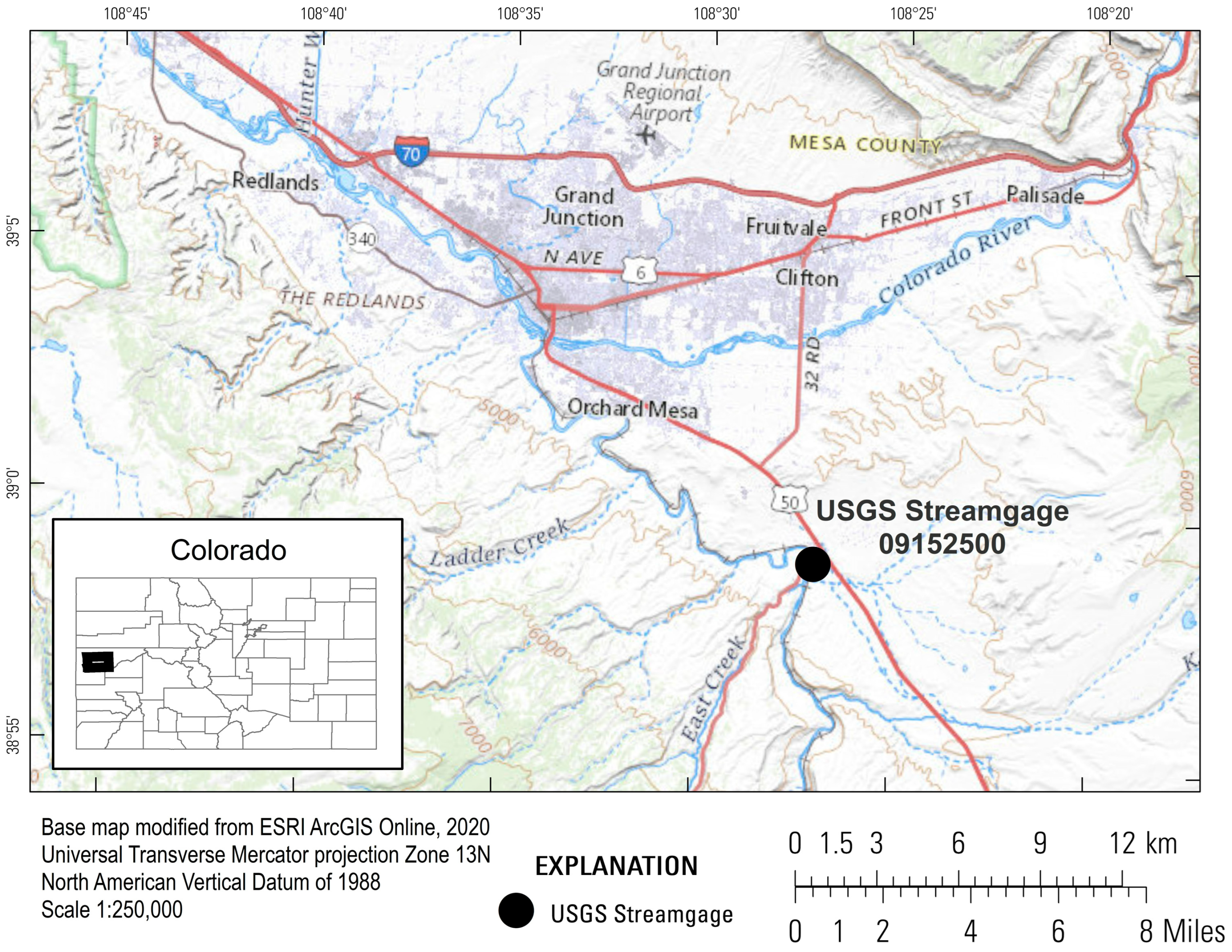

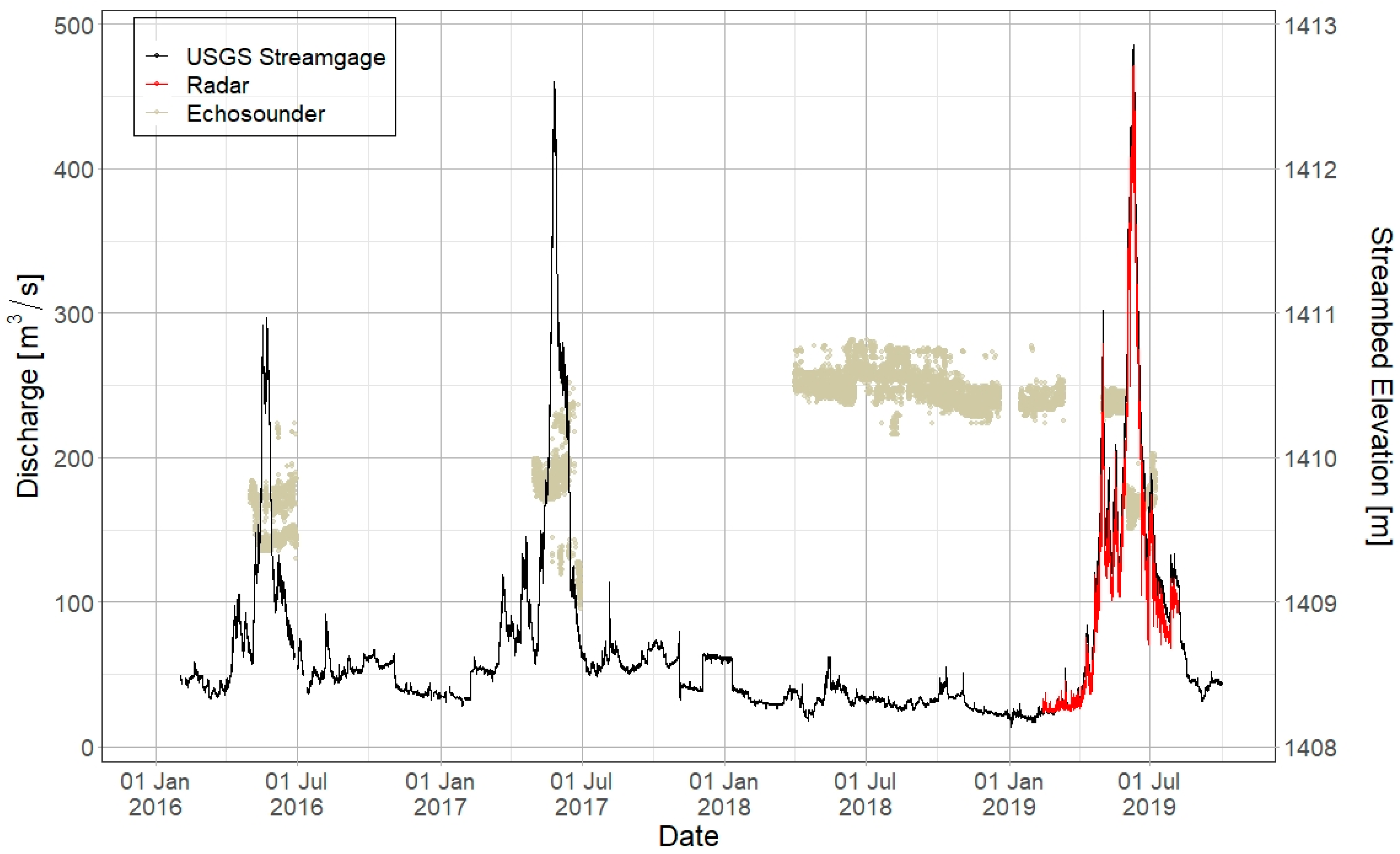
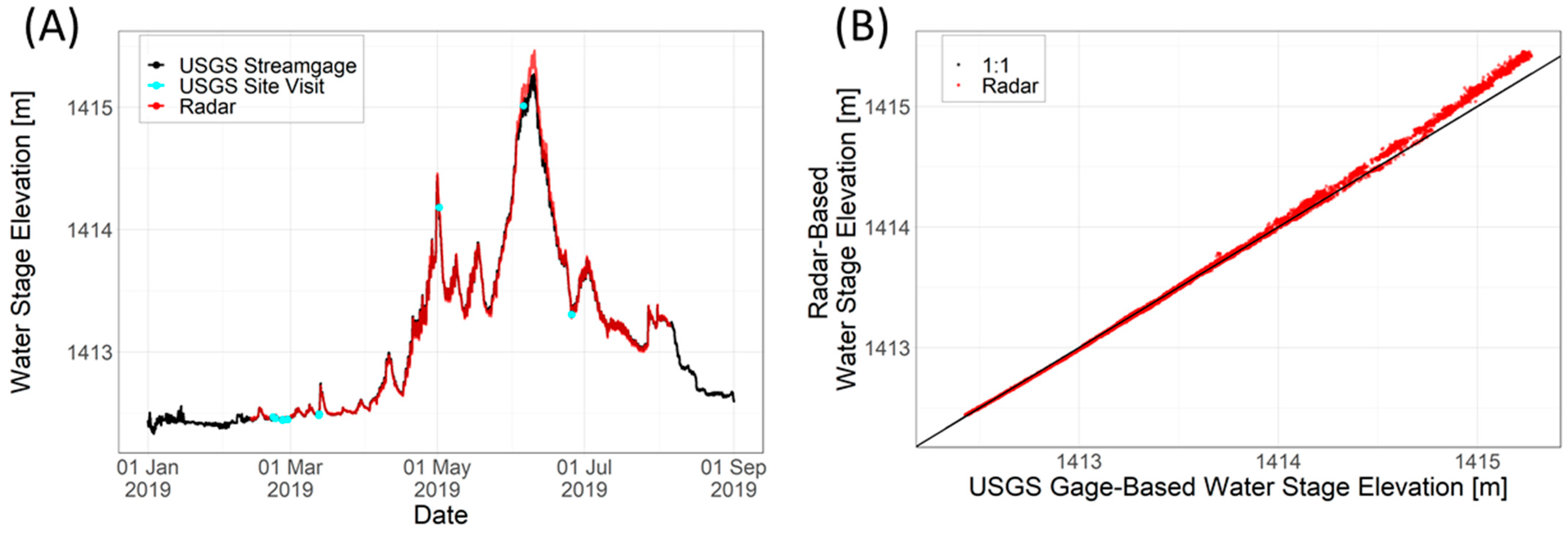
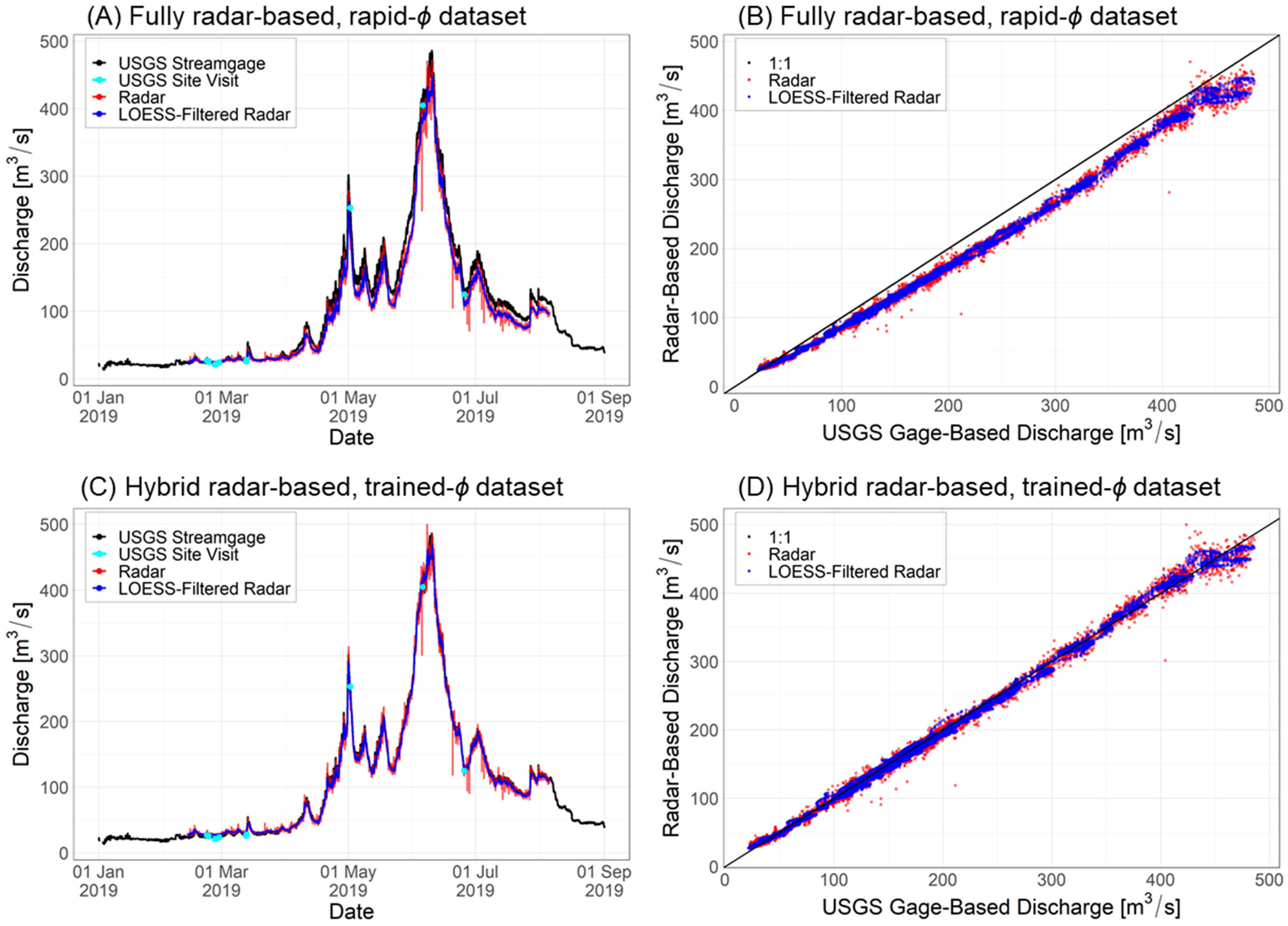
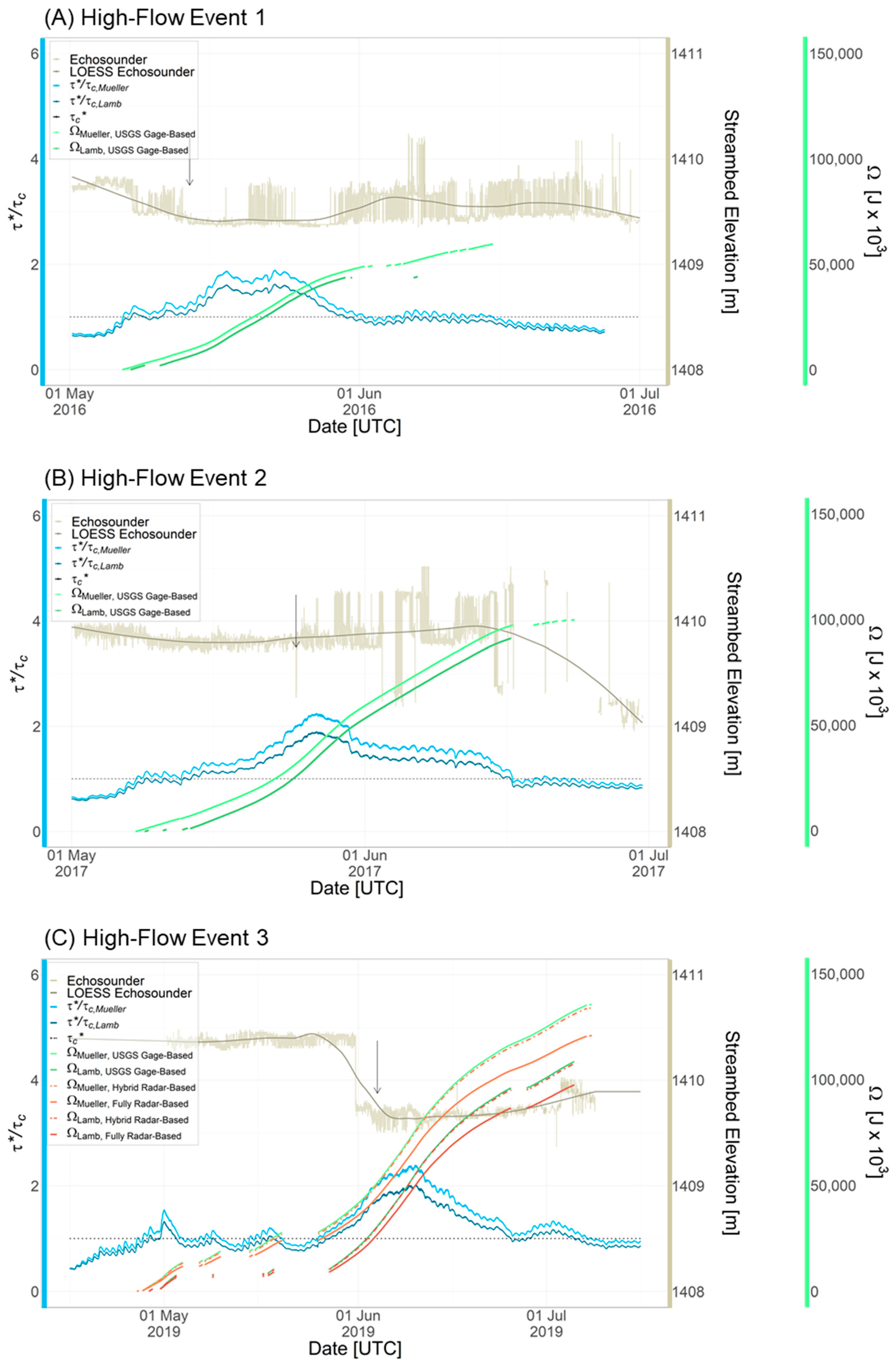
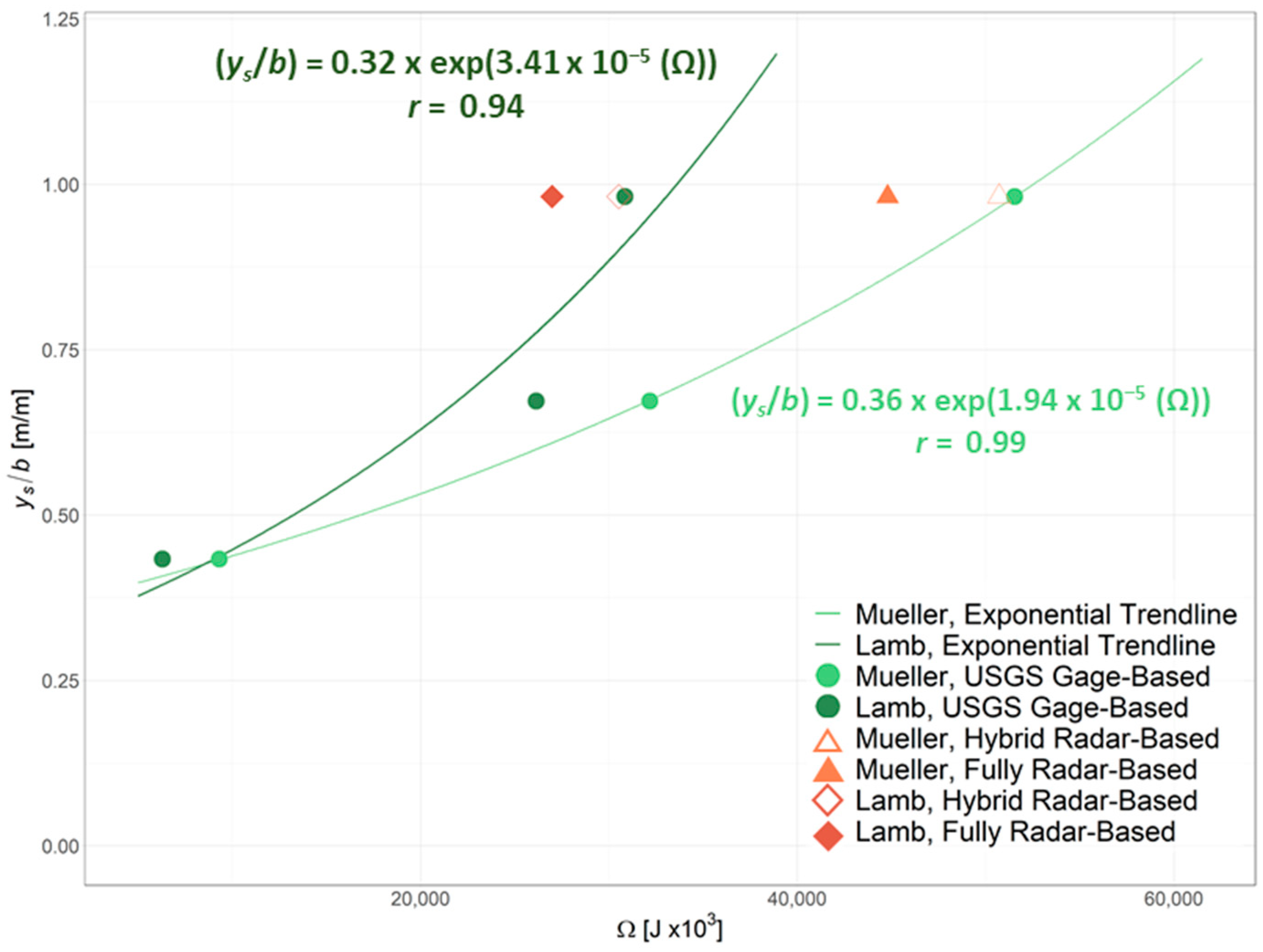
Publisher’s Note: MDPI stays neutral with regard to jurisdictional claims in published maps and institutional affiliations. |
© 2022 by the authors. Licensee MDPI, Basel, Switzerland. This article is an open access article distributed under the terms and conditions of the Creative Commons Attribution (CC BY) license (https://creativecommons.org/licenses/by/4.0/).