Article

Land Use and Land Cover Mapping Using Sentinel-2, Landsat-8 Satellite Images, and Google Earth Engine: A Comparison of Two Composition Methods

by
Vahid Nasiri
1,
Azade Deljouei
2,*,
Fardin Moradi
1,
Seyed Mohammad Moein Sadeghi
2 and
Stelian Alexandru Borz
2
1
Department of Forestry and Forest Economics, Faculty of Natural Resources, University of Tehran, Karaj 14176-43184, Iran
2
Department of Forest Engineering, Forest Management Planning and Terrestrial Measurements, Faculty of Silviculture and Forest Engineering, Transilvania University of Brasov, Şirul Beethoven 1, 500123 Brasov, Romania
*
Author to whom correspondence should be addressed.
Remote Sens. 2022, 14(9), 1977; https://doi.org/10.3390/rs14091977
Submission received: 29 March 2022 / Revised: 15 April 2022 / Accepted: 18 April 2022 / Published: 20 April 2022
(This article belongs to the Special Issue Remote Sensing of Land Use and Land Change with Google Earth Engine)

Abstract

:
Accurate and real-time land use/land cover (LULC) maps are important to provide precise information for dynamic monitoring, planning, and management of the Earth. With the advent of cloud computing platforms, time series feature extraction techniques, and machine learning classifiers, new opportunities are arising in more accurate and large-scale LULC mapping. In this study, we aimed at finding out how two composition methods and spectral–temporal metrics extracted from satellite time series can affect the ability of a machine learning classifier to produce accurate LULC maps. We used the Google Earth Engine (GEE) cloud computing platform to create cloud-free Sentinel-2 (S-2) and Landsat-8 (L-8) time series over the Tehran Province (Iran) as of 2020. Two composition methods, namely, seasonal composites and percentiles metrics, were used to define four datasets based on satellite time series, vegetation indices, and topographic layers. The random forest classifier was used in LULC classification and for identifying the most important variables. Accuracy assessment results showed that the S-2 outperformed the L-8 spectral–temporal metrics at the overall and class level. Moreover, the comparison of composition methods indicated that seasonal composites outperformed percentile metrics in both S-2 and L-8 time series. At the class level, the improved performance of seasonal composites was related to their ability to provide better information about the phenological variation of different LULC classes. Finally, we conclude that this methodology can produce LULC maps based on cloud computing GEE in an accurate and fast way and can be used in large-scale LULC mapping.

Graphical Abstract

1. Introduction

Land use maps are fundamental data sources for land planning and management [1,2]. Accurate and up-to-date land use/land cover (LULC) mapping has always been of interest to geoscience and remote sensing societies [3,4,5], mainly because it is a provider of valuable information to understand human–environment relationships [6,7]. The starting point for LULC mapping was that of using mono-temporal and mono-source satellite images [8]. For these approaches, spectral and textural features played a substantial role in improving the classification results [9,10] and the efforts continued with the combined use of multi-source datasets, such as those integrating optical and radar satellite images [11,12]. Previous studies attempted to integrate different types of remotely sensed data and to use their unique capabilities to produce accurate LULC maps. For example, Clerici et al. [13] reported that optical and radar Sentinel data provide supplementary information; therefore, LULC classification can take advantage of the integration of both data sources leading to an increase in classification accuracy. The development and global consolidation of remotely sensed data [14,15], cloud computing platforms [16,17,18], time series-based approaches [19,20] and artificial intelligence, machine learning, deep learning, and deep transfer learning [21,22,23,24,25] provided new insights into the field of large scale LULC mapping. Cloud computing platforms such as Google Earth Engine (GEE) and Framework for Operational Radiometric Correction for Environmental monitoring (FORCE) provide high computing power and accessibility to dense time series [16,26,27]. GEE provides various satellite data and satellite-derived products through its data catalog [28]. Those using GEE platforms can avoid storing images locally and access greater computing power to analyze and process images [29].
Analyzing time series of satellite imagery enables the integration of a diverse set of features and spectral–temporal metrics to capture seasonal and phenological characteristics of various LULC classes [30,31,32]. The application of such features and metrics to mapping LULC classes has increased the classification accuracy [33,34]. Among the medium resolution satellite images, Landsat-8 (L-8) and Sentinel-2 (S-2) products provide high temporal resolution data, short revisit time, and rich spectral configuration, making them appropriate sources for time series feature extraction [35,36]. Generally, three methods are used to extract time series features and to manage missing data: (1) time series composition, (2) spectral–temporal metrics, and (3) phenological metrics [37,38].
Composition methods convert all images into a single image covering a given time window (annual, seasonal, etc.). Each pixel in the resulting image represents the reflectance of all pixels from the original image collection based on defined roles. The most important benefit of this method is that of reducing the atmospheric effects, such as cloud and snow masking [39]. Spectral–temporal metrics produce statistical spectral information of all pixels along a time scale. These metrics can be produced based on the mean, standard deviation, maximum, minimum, or percentiles of spectral information during the defined period [40]. Phenological metrics are generated based on the periodicity of land cover classes, such as the date of start, peak, and end of the growing season and they represent well the phenological variation of different LULC classes or vegetation types [41]. In this regard, Azzari and Lobell [42] used both seasonal composites and 0.1, 0.25, 0.5, 0.75, and 0.90 quintile spectral–temporal metrics and achieved 89% overall accuracy in cropland mapping. Phenological metrics are mainly used in the mapping of vegetation types. Hemmerling et al. [43] reported that using phenological metrics extracted from dense S-2 time series helped mapping different forest tree species. Xie et al. [44] assessed the capabilities of percentile metrics and monthly composites in large-scale LULC mapping to identify which methods would produce more accurate results. The importance of cloud computing platforms and time series feature extraction methods becomes evident when there is a need to process large amounts of data and a high number of features for accurate and large-scale LULC mapping [45,46].
Moving to the context of the analysis, most of the previous studies used time series spectral–temporal metrics to capture detailed characteristics of LULC classes and to build powerful models for accurate LULC prediction. Most of the previous LULC mapping studies used mono source satellite time series and a single method for time series feature extraction [47,48]. Some studies used several methods for time series feature extraction but on mono-source satellite data [49]. The novelty of this study is that it aimed at comparing two commonly used time series feature extraction methods, namely, seasonal composites and percentile metrics, and evaluating their performance in large-scale LULC mapping based on two sources of data, namely, S-2 and L-8 time series. The above-mentioned approach to the problem was operationalized by using a random forest (RF) machine learning classifier. Hence, the objectives of this study were the following: (1) evaluating the effect of two composition methods (i.e., percentile and seasonal) on LULC mapping accuracy, (2) comparing the performance of data provided by S-2 and L-8 satellite images in LULC mapping, and (3) identifying the most suitable variables for LULC prediction.
The rest of the paper is organized as follows. In Section 2, the study area, datasets, and methodologies of LULC classification and accuracy assessment are described. The results and analyses are presented in Section 3. A discussion is presented in relation to other studies in Section 4, and finally, the paper concludes in Section 5.

2. Materials and Methods
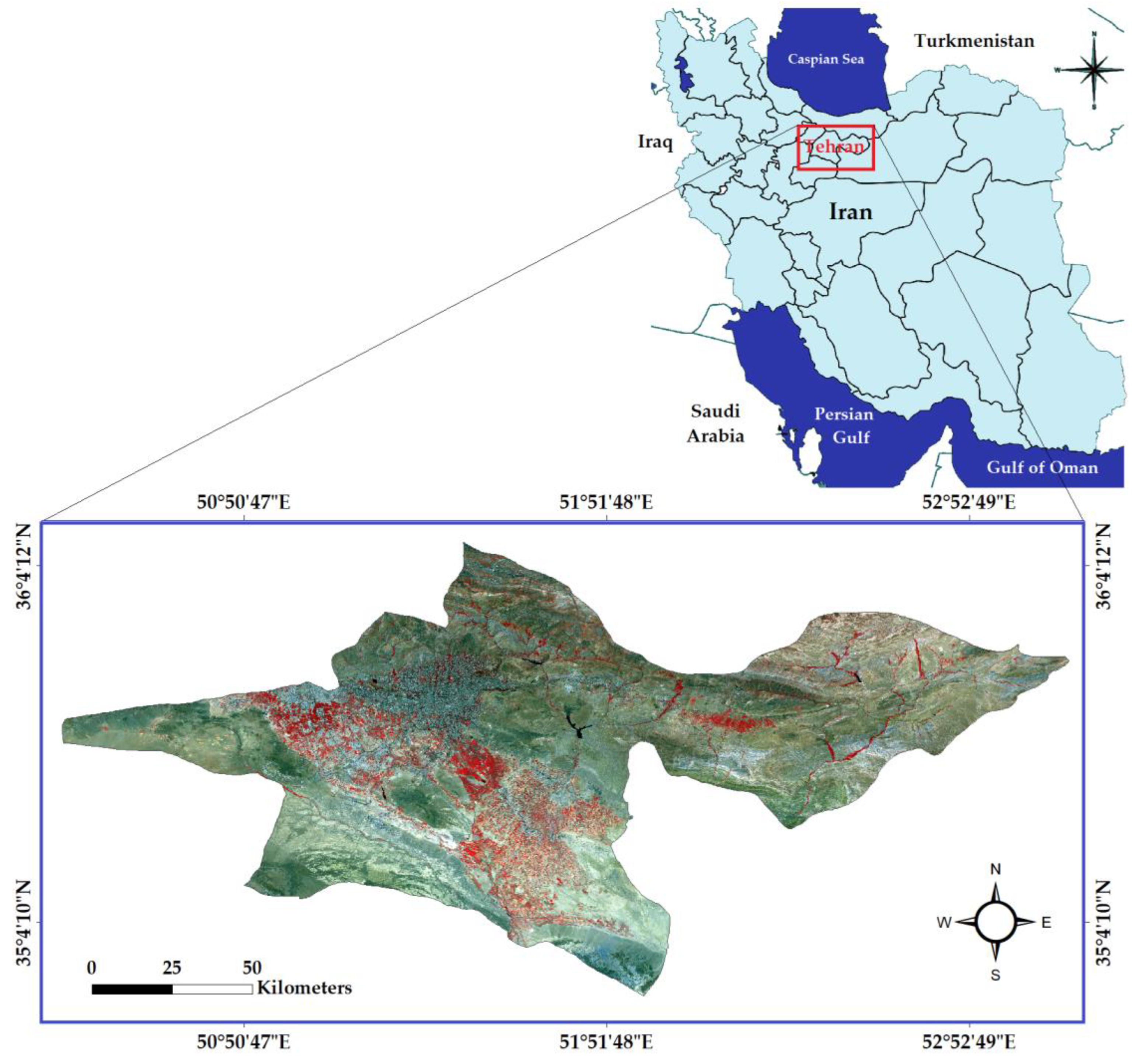
2.1. Study Area

This study was carried out in the Tehran Province, including Tehran city and its suburbs, covering an area of 14,000 Km2 located in the northcentral part of Iran at the southern face of the Alborz Mountains (Figure 1), spanning over 34° to 36°5′N and 50° to 53°E. This region is the most industrialized region in the country and has the highest population density (11,800 individuals/km2) which is mainly concentrated in 10 cities. In general, this province is characterized by an arid climate [7,50] being cold and semi-humid in the northern areas and cold with long winters in the higher regions. Grasslands are located in the northern and western parts, while croplands and bare lands are mainly found in the southern and eastern parts of the region. The boundary of the study area was chosen in a way that could well represent a complex landscape and involved densely built-up and suburban residential areas, industrial cities, croplands, woodlands, grasslands, and bare lands.

2.2. Datasets

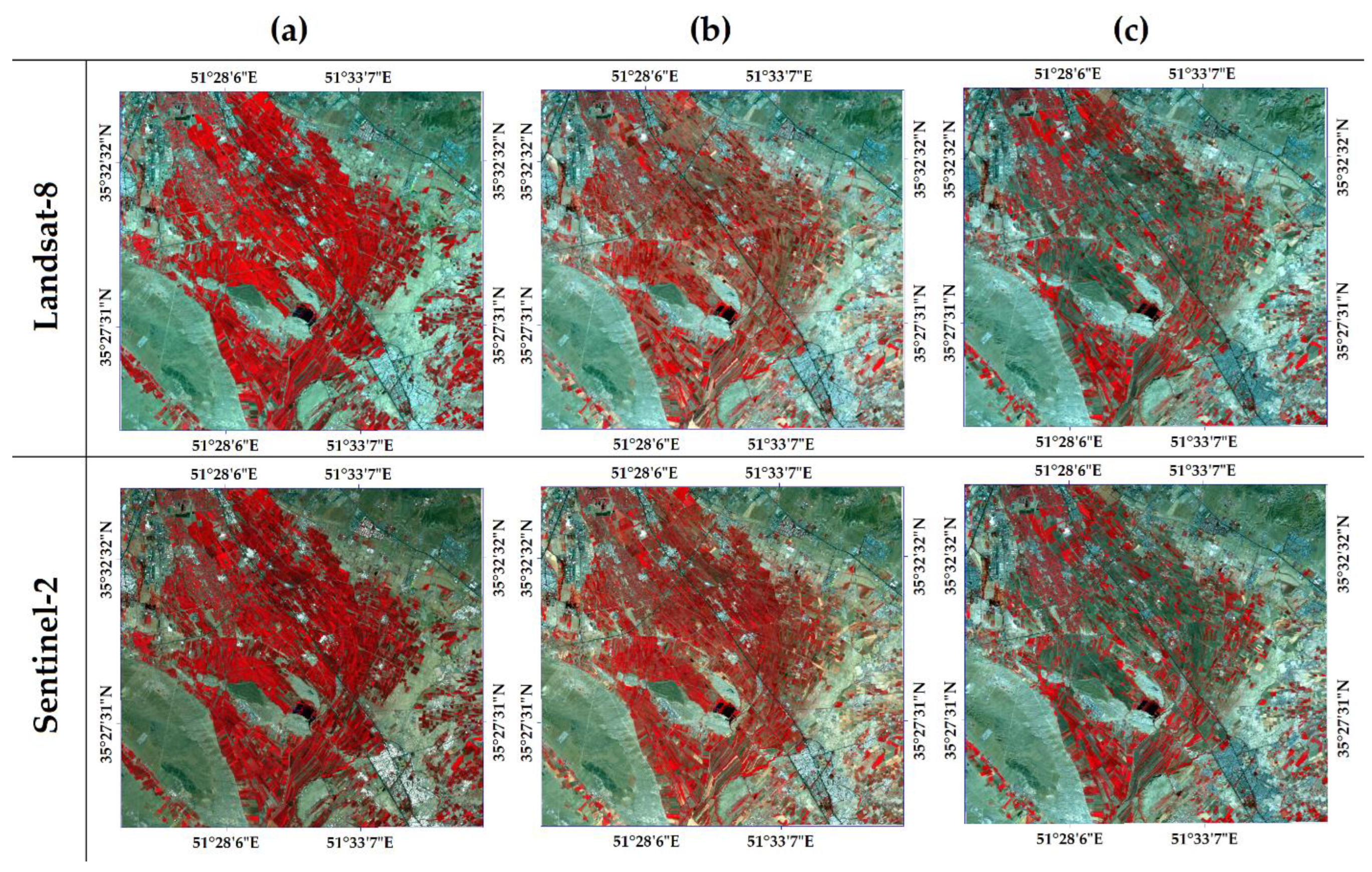
2.2.1. Satellite Data

In this study, the S-2 and L-8 Operational Land Imager (OLI) time series data were used for mapping the LULC classes. The L-8 OLI consists of nine spectral bands (coastal: 443 nm, blue: 485 nm, green: 563 nm, red: 655 nm, panchromatic: 640, NIR: 865 nm, short-wave infrared 1 (SWIR1): 1610 nm, SWIR2: 2200 nm, and cirrus: 1375 nm) (https://www.usgs.gov/landsat-missions/landsat-8; accessed on 14 December 2021). S-2 provides high temporal resolution data with a rich spectral configuration, including 13 spectral bands. It has six land monitoring bands that are comparable with Landsat-8 (blue: 490 nm, green: 560 nm, red: 665 nm, NIR: 842 nm, SWIR1: 1910 nm, and SWIR2: 2190 nm) and three additional bands covering the red-edge part of the spectrum which are centered at 705 nm, 740 nm, and 783 nm, and a NIR narrow band at 865 nm (https://sentinel.esa.int/web/sentinel/missions/sentinel-2; accessed on 14 December 2021).

2.2.2. Digital Elevation Model

Shuttle radar topography mission (SRTM) digital elevation model (DEM) with a resolution of 1 arc second (approximately 30 m) was used to extract the elevation and slope bands. The SRTM resulted from international cooperation between the National Aeronautics and Space Administration (NASA), the National Geospatial-Intelligence Agency (NGA), and German and Italian space agencies. SRTM provides a near-global DEM between 60°N and 56°S latitude, built on the data collected by a specially modified radar system onboard the Space Shuttle Endeavour (SSE) during 11 days in February 2000 (https://lpdaac.usgs.gov/products/srtmimgmv003/; accessed on 14 December 2021). Since all L-8 30 m and SRTM 30 m spatial resolution datasets were used in the analysis, all the bands were resampled to 10 m (S-2 resolution) and registered to match the S-2 georeferenced images. Moreover, in GEE, the scaling is executed automatically and all the bands are overlaid perfectly.

2.2.3. Reference Datasets and LULC Classes

In this study, the attempt was to develop an appropriate methodology to achieve the specific research objectives outlined above. Four datasets were prepared so as to be characterized by different time series feature set configurations based on S-2 and L-8 satellite images and two common composition methods. Generally, a high classification accuracy of the remotely sensed datasets requires large sets of training and validation samples. Therefore, a second step was that of generating a high number of training and validation samples to properly manage the issues of insufficient sample sizes and large numbers of dimensions [51,52]. Based on the above, an RF classifier was used to produce LULC maps and to evaluate the classification accuracy by a set of metrics. Since the accurate mapping of LULC classes based on machine learning methods requires a sufficient number of training samples [53], a visual inspection of high-resolution satellite imagery is a typical method used to extract training and validation samples [54,55]. In this study, a number of 3800 ground polygon samples (33,530 pixels) were defined based on a random distribution within LULC classes which included artificial land, cropland, woodland, grassland, bare land, and water bodies; this was done by a visual interpretation of the Google Earth high-resolution satellite imagery (Table 1). The characteristics of LULC classes are described in Table 1. Some studies indicated that the reference datasets should represent approximately 0.25% of the total study area [56,57]. Therefore, we used this proportion to collect our samples in each LULC class and there was an imbalance between them. All the samples were divided into training (60%) and validation (40%) subsets.

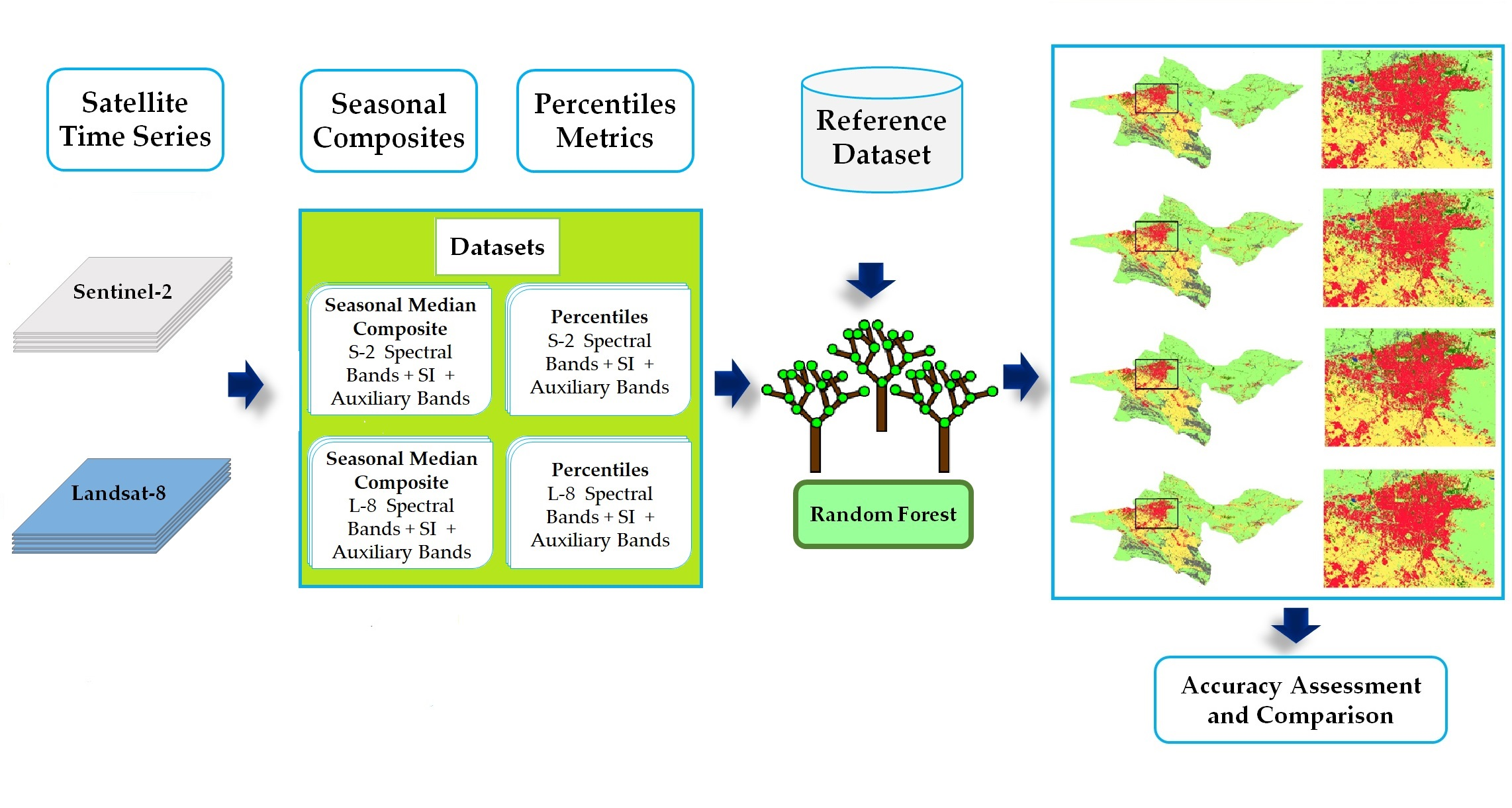
2.2.4. Time Series Image Analysis

The GEE cloud computing platform (https://earthengine.google.com; accessed on 14 December 2021) [16] was used to create image collections and process the time series. All of the 2020 S-2A/B level 2A and L-8 OLI surface reflectance products over the study area were processed to extract spectral–temporal metrics as predictors for LULC classification. All images with less than 30% cloud cover were filtered as a beginning step. After that, we used the S2cloudless algorithm (for S-2 images) and the function of mask (FMASK; for L-8 images) for masking pixel-wise cloud, cloud shadow, and snow from image collections. During the masking process for both satellites, the results were visually inspected and all parameters were redefined until the best result was obtained [58].
For the extraction of spectral–temporal metrics, two methods were considered to meet the research goals:
  • Seasonal composites method: The median reducer was used to generate cloud-free seasonal composites [59]. Satellite images were filtered based on the climatological regime from the North of Iran, and took into consideration three seasons: spring (March, April, and May), summer (June, July, and August), and autumn (September, October, and November). Images from winter were discarded because of the high amounts of clouds and snow cover. This method was aimed at including the phenological information in LULC classification [60].
  • Percentile metrics method: For each image collection, the percentile metric method constructs the histogram of feature collection and then calculates the specified percentiles of the feature distribution [61]. In this study, all the images from 2020 (March to November) were used to produce the 0.1, 0.25, 0.5, 0.75, and 0.95 percentile-based metrics for all spectral bands and indices.
In addition to the spectral bands, the following spectral indices were calculated: normalized difference vegetation index (NDVI; [62,63]), normalized difference built-up index (NDBI; [64,65]), and green normalized difference vegetation index (GNDVI; [66,67]). The spectral–temporal metrics were calculated (Table 2) by using the aforementioned strategy. In the classification process, these topography-based features were used to include the terrain attributes of the LULC classes [68].

2.2.5. Land Cover Classification and Accuracy Assessment

A number of 2280 ground polygon samples (Section 2.2.3) were used to extract per-band pixel values of the four composited datasets. These samples were used to train the RF classifier. RF is an ensemble learning method based on a combination of decision trees [69]. This classifier was also found to perform better compared with other machine learning (ML) classifiers such as support vector machine (SVM) [70]. RF requires less processing time, fewer parameters, and minimal manual intervention compared with SVM [71,72]. It can also cope properly with multi-modal data [73] and implicitly performs spectral selection due to its underlying principle [69]. Based on previous findings [74,75], a RF classifier with 500 decision trees (i.e., ntree) was trained and tested on each dataset described in Table 2 to create LULC classifications. The assessment of classification accuracy was carried out by comparing the LULC classes resulted from the training phase with data yielded by the testing phase (numbers of ground polygon samples = 1520) using for this purpose confusion matrices. Based on the confusion matrices, global quality metrics such as the overall accuracy (OA) and kappa coefficient (K) were calculated (Equations (1) and (2)) to evaluate the impact of composition methods on LULC classification.
Overall   Accuracy   OA = Number   of   Correctly   Classified   Samples Number   of   Total   Samples
Kappa = Overall   Acuuracy Estimated   Chance   Agreement 1 Estimated   Chance   Agreement
Moreover, the class level consumer’s accuracy (CA), producer’s accuracy (PA), and F1-score were calculated (Equations (3)–(5)). The F1-score is the harmonic mean between producer’s and user’s accuracies and can be used to evaluate the accuracy at class level [76].
CA = Number   of   Correctly   Classified   Samples   in   each   Class Number   of   Samples   Classified   to   that   Class
PA = Number   of   Correctly   Classified   Samples   in   each   Class Number   of   Samples   from   Reference   Data   in   each   Class
F 1 = 2 × CA   × PA CA + PA
PA is the probability that a pixel was correctly classified in a given class. CA is the probability that a pixel classified in a given class of the map represents that class on the ground [77]. The F1 was found to be the best performance metric and is widely used in previous research, which gives equal importance to both PA (as a precision) and CA (as a recall) by combining them into a single model performance metric [78,79]. The methodology adopted in this study is provided in the flowchart shown in Figure 2.

2.2.6. Variable Importance

Variable importance stands for the variables’ contribution to distinguish between LULC classes, which helps by improving the classification accuracy while reducing data redundancy and processing workload. In this study, variable importance was derived from the RF model to estimate the contribution of variables (i.e., spectral bands and indices) to the obtained accuracy of the model [80].

3. Results

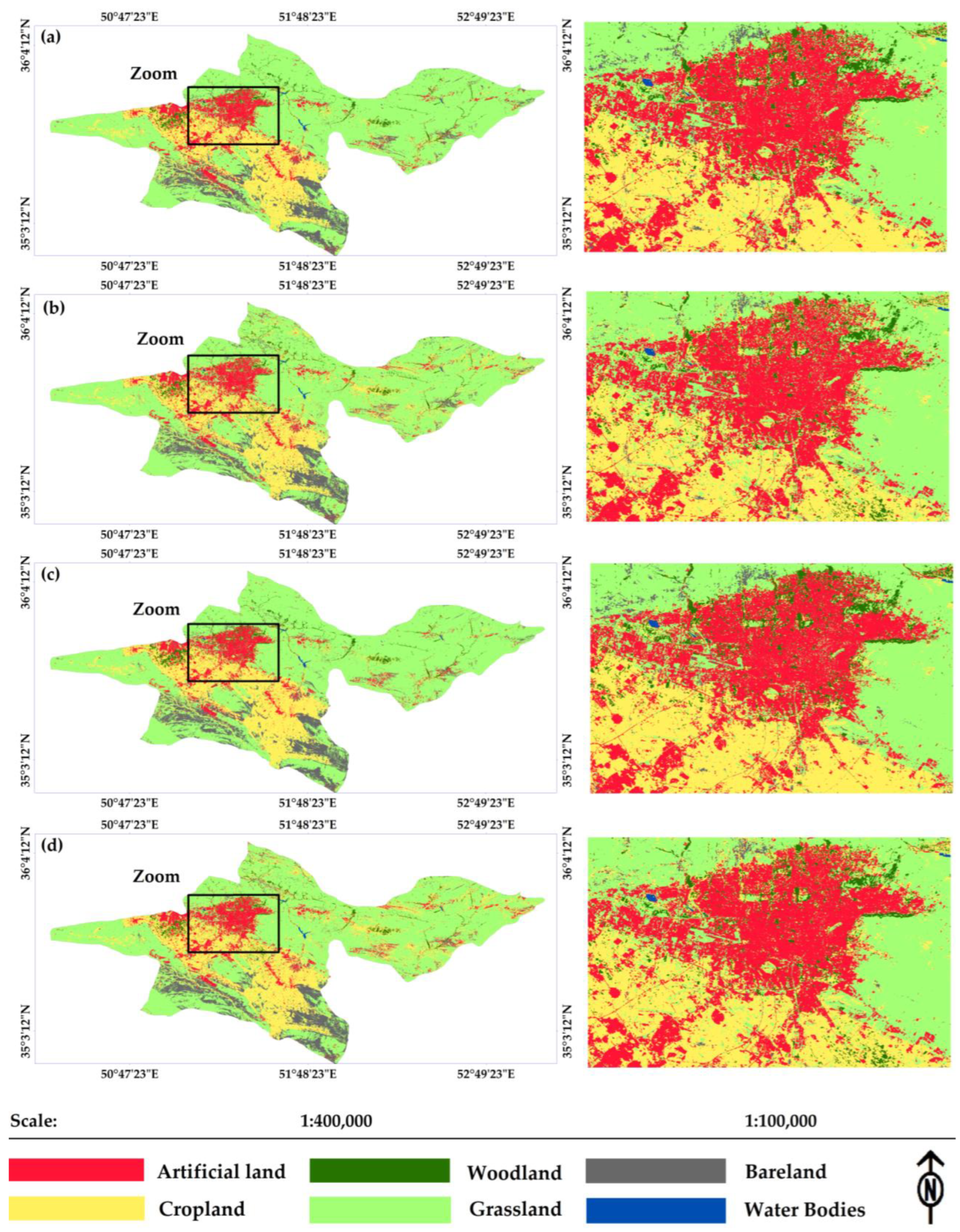
3.1. LULC Maps and the Overall Accuracy

Figure 3 shows the LULC maps resulting from the four datasets based on the S-2 and L-8 spectral–temporal metrics.
The accuracy figures reached by the four datasets characterizing different composition methods are provided in Table 3. Based on the results, the overall accuracy of all datasets was relatively close. The highest overall accuracy and K coefficient were reached by the S-2 seasonal composites (OA = 95.48%, K = 0.9387), closely followed by S-2 percentile metrics (OA = 95.34%, K = 0.9365), L-8 seasonal composites (OA = 94.30%, K = 0.9220), and L-8 percentile metrics (OA = 93.87%, K = 0.9116). Therefore, in terms of satellite images, the highest overall accuracy and K coefficient were reached by S-2 using seasonal and percentile composites. Moreover, seasonal composites produced slightly higher accuracies than percentile metrics (Table 3).
Figure 4 provides some false color composites with their associated seasonal composites to better evaluate the effect of phenological information for an accurate LULC classification. As observed, the phenological variation of LULC classes, particularly of croplands and woodlands, was provided effectively via seasonal composites.

3.2. Class Level Accuracy Assessment

For a more in-depth evaluation, per-class producer (PA) and consumer (CA) accuracies and F1-scores are provided for all datasets in Table 4. Regarding the role of time series composition methods, for both S-2 and L-8 datasets, it can be observed that the CA, PA, and F1 scores were higher in all LULC classes when using seasonal composites rather than percentile metrics. The lowest CA, PA, and F1-score were calculated for bare lands and the highest ones were observed for water bodies in all datasets.
The highest CA, PA, and F1-scores for all LULC classes were produced by dataset-1 (except grasslands). In contrast, dataset-4 had lower CA, PA, and F1 score values of all LULC classes (except grasslands). As observed in Table 4, the CA, PA, and F1 score values of artificial lands (AL) in all datasets were very high (F1-score ranged between 97.62 and 94.48%) and there were no contrasting differences between different datasets. Similar results were also observed in terms of woodland (WO) classification (F1-score varied between 95.54 and 94.52%), with the exception that PA values for all datasets were quite low (ranged between 93.18 and 92.16%). There were some omission errors in the woodland classification. Regarding the cropland (CR) classification, S-2 based datasets (seasonal composites and percentiles metrics) achieved higher CA, PA, and F1-score values than the L-8 datasets. A similar difference in accuracy was observed by comparing the values returned by the composition methods used for each satellite time series. The F1-scores produced for cropland based on S-2 and L-8 datasets (seasonal and percentiles) were of 95.55 and 94.06%, respectively. Based on the results (Table 3), the lowest CA, PA, and F1-score values were calculated for bare land in all datasets. The results also showed that the S-2 datasets had a higher capability of mapping bare lands than L-8 datasets. For example, the CA and PA values produced for bare land using S-2 seasonal composites (dataset-1) increased by nearly 8% and 7%, respectively, as opposed to L-8 seasonal composites (dataset-3). Moreover, an important difference was observed in CA, PA, and F-1 scores of bare land classification between these datasets. These differences were also observed between dataset-2 (S-2 percentiles) and dataset-4 (L-8 percentiles). In terms of grassland classification, the best result was obtained with dataset-2, in which we used S-2 percentiles. But there were no remarkable differences between all datasets in grassland mapping accuracy.
Figure 5 provides some finer-scaled partitions of the maps to better evaluate the differences between the datasets in identifying LULC classes. As shown, there were problems in all datasets to distinguish between bare and artificial land, grassland, and harvested croplands, which remain challenging to differentiate due to similar spectral properties.

3.3. Variable Importance

In all datasets, elevation, slope, and vegetation indices were found to be the most important variables in RF models (Figure 6). In regard to S-2 seasonal composites, S-2 new spectral bands such as B8A, B5, and B6 were among the most important variables. In the case of L-8 seasonal datasets (datasets 3 and 4), in addition to vegetation indices, spectral bands including B5, B4, and B2 had a higher importance than other bands in LULC prediction.

4. Discussion

Spatial distribution of LULC classes is often related to topographic factors [9,81]. Therefore, we considered elevation and slope factors in training and testing the RF models. As a result, in all RF models, elevation factors obtained high importance scores. The importance of topographic variables in large-scale LULC classification was also reported in similar studies [39,82]. For example, Rufin et al. [83] used topographic factors (elevation and slope) in their LULC model and indicate their high importance in increasing the overall accuracy. In another study, Htitiou et al. [30] used elevation and slope layers in the attempt to map croplands at national scale. Based on their results, these variables improved the ability to distinguish croplands, particularly in regions characterized by high elevation and steep slopes. Phan et al. [84] defined several datasets based on L-8 time series and auxiliary bands such as topographic factors and reported that the elevation was the most important variable in all of the models. Therefore, the high importance of topographic factors used in this study was consistent with the results reported by previous studies.
Regarding the composition methods used for S-2 and L-8 time series, the results showed that seasonal composites outperformed percentile metrics in distinguishing different LULC classes. In terms of accurate LULC mapping, the strategy used to generate composites depends on the types of LULC classes and the density of available time series [44]. The higher performance of seasonal composites in this study can be related to the selected LULC classes which covered cropland, woodland, and grassland. The use of seasonal composites enabled the inclusion of phenological information. These kinds of seasonality features were a piece of sufficient and valuable information for distinguishing the LULC classes with similar spectral attributes. The importance of phenological information was also reported in similar studies. Xie et al. [44] defined two datasets based on monthly median composites and percentile metrics to classify different LULC classes including various types of vegetation such as evergreen forests, deciduous forests, shrublands, croplands, etc., using Landsat TM/ETM+ time series and reported that the highest overall accuracy was produced by using monthly median composites.
When comparing the two satellite time series, accuracy assessment results indicated that S-2 composition methods (seasonal composites and percentiles metrics) produced higher accuracies than their L-8 counterparts did. The L-8 time series used in this study had similar spectral features to S-2 time series, excluding the red-edge bands of S-2. Therefore, the better results provided by the S-2 could be related to the red-edge bands and their spectral–temporal metrics. The feasibility and efficiency of red-edge bands were also present in variable importance scores. As Figure 6 illustrates, in both seasonal and percentile composites, red edge bands (B-7, 6, and 5) played a significant role in the performance of the RF classifier. Forkuor et al. [85] defined several datasets with different feature configurations based on mono date S-2 and L-8 bands. Based on their results, the S-2 dataset produced the highest accuracy. To evaluate the effect of red edge bands on the classification results, they also added S-2 red edge bands to the L-8 dataset and reported a 4% improvement compared with L-8 bands. Moreover, Immitzer et al. [86] reported that red-edge bands, particularly B-5 (RE1), are among the most important data features in mapping vegetation types such as croplands and woodlands. Ghayour et al. [87] compared the performance of S-2 and L-8 satellite images in LULC mapping by using classifiers such as SVM, artificial neural network (ANN), maximum likelihood classification (MLC), minimum distance (MD), and Mahalanobis distance (MHD). According to their findings, S-2 produced higher accuracies compared with the L-8 datasets irrespective of the classifier used.
Analyzing the confusion matrices indicated that bare lands were poorly identified and most of them were classified as grasslands. Moreover, some pixels of the bare land were misclassified as artificial lands. This problem occurred more often in the L-8 based datasets (dataset-3 and dataset-4). Therefore, the largest difference between the S-2 and L-8 composites was that observed in the classification of bare lands. The classification of bare lands, on the other hand, is a common challenge in LULC mapping studies. Zhao and Zhu [88] reported that some LULC classes such as artificial lands, bare lands, deserts, and harvested croplands have similar spectral signatures and tried to develop a spectral index to better distinguish these classes. They introduced the artificial surface index (ASI) by considering the artificial surface enhancement, vegetation, and bare soil suppressing and reported that ASI could increase the separability of artificial lands from other types of land use. Ettehadi Osgouei et al. [89] faced the same challenge and tried to use spectral indices, including the normalized difference tillage index (NDTI), red-edge based NDVI, and modified normalized difference water index (MNDWI). They reported that these spectral indices could improve the performance of the SVM classifier to distinguish bare land from urban areas. We used similar spectral indices in this study, including the NDVI, GNDVI, and NDBI, but it seems that this challenge still remains. Nevertheless, these spectral indices showed a good performance in differentiating other classes with similar spectral signatures, such as woodland and dense croplands.
In this study, croplands were composed of irrigated and rain-fed crops, which hold heterogeneous spectral patterns [90]. Considering all these spectral similarities and heterogeneous patterns, our approach and the used spectral–temporal metrics could enhance the classification accuracy. In some studies, the integrated use of textural and spectral features was found to be a solution to distinguish LULC classes with similar spectral properties. For example, Petrushevsky et al. [91] integrated S-2 multispectral bands, Sentinel-1 texture features, and object-based image analysis to generate an urban mask and reached a 90% overall accuracy. The radar signal is sensitive to geometry (e.g., roughness, texture, and internal structure), while physiology influences optical reflectance [92]. As such, these two spectral domains may provide complementary information [93]. Hence, the integration of radar time series and textural feature is recommended for future research [94,95].
Under the GEE platform, the satellite image processing time can be greatly shortened, which helps users to store decades of data and removes the need to download the satellite images one by one. However, one of the limitations of our study was the limited availability of data with suitable resolution in the Google Earth catalog, whose improvement in this direction is desirable for both researchers and practitioners. The second limitation of this study was the lack of precise training and validation samples, making it impossible for us to conduct our study on a much larger scale. These samples were collected automatically from existing reference datasets such as the land use/cover area frame survey (LUCAS) in similar studies. There was no access to accurate reference datasets or reliable LULC maps in our study area. Therefore, we used very high resolution (VHR) satellite images provided by Google Earth and visual interpretation, which are very time-consuming and challenging, particularly when dealing with large areas. Moreover, based on the previous studies and our results, topographic bands (such as elevation and slope) are very important variables in increasing the overall accuracy. In this study, we used freely available SRTM DEM with a resolution of approximately 30 m. Considering the importance of topographic variables, using more accurate DEMs could considerably increase the classification results. Unfortunately, we didn’t have access to such high-resolution DEM in this study (third limitation). Therefore, future studies could use more accurate DEM, especially when dealing with mountainous landscapes. Future research may compare the existing land use products, such as those from this paper, with global products (e.g., ESA WorldCover and GlobCover maps). Since the classification accuracy may be affected by the type of machine learning model used, future studies could compare the results of other popular classifiers for LULC mapping such as SVM, ANN, and deep learning models. Finally, we suggest comparing balanced and imbalanced reference datasets in terms of classification accuracy as well as considering larger study areas with different climate conditions.

5. Conclusions

This study aimed at evaluating the potential of S-2 and L-8 time series and the RF classifier to produce accurate LULC maps. The S-2 and L-8 time series were used to generate spectral–temporal metrics based on two composition methods (seasonal and percentiles) to achieve the research objectives. Datasets, including S-2 and L-8 spectral temporal metrics and vegetation indices were defined, then their performance in identifying six common LULC classes (artificial land, water bodies, woodland, cropland, bare land, and grassland) was compared. The study concludes that medium resolution satellite time series and the extracted spectral–temporal metrics are robust sources for accurate LULC mapping. However, some differences among the datasets were observed. For instance, the LULC maps generated from the S-2 time series were more accurate than those generated from the L-8 time series. The comparison between composition methods indicated that seasonal median composites outperformed percentile metrics in both S-2 and L-8 time series. The results proved the efficiency of vegetation indices, particularly of NDVI and NDBI and S-2 red-edge bands, concerning the variable importance. In short, the approach used in this research and the generated spectral–temporal metrics can be used to produce accurate LULC maps based on the GEE cloud computing platform. These results highlight that cloud computing platforms such as GEE and new Earth-observing satellites such as S-2 have contributed significantly in improving LULC mapping and monitoring.

Author Contributions

Conceptualization, V.N., A.D., F.M. and S.M.M.S.; data curation, V.N. and A.D.; formal analysis, V.N., A.D. and F.M.; funding acquisition, A.D., S.M.M.S. and S.A.B.; investigation, V.N.; methodology, V.N., A.D., F.M. and S.M.M.S.; software, V.N. and A.D.; supervision, A.D. and S.M.M.S.; visualization, V.N. and S.M.M.S.; writing—original draft, V.N.; writing—review and editing, A.D., S.M.M.S. and S.A.B. All authors have read and agreed to the published version of the manuscript.

Funding

This research received no external funding and the APC was funded by the Department of Forest Engineering, Forest Management Planning, and Terrestrial Measurements.

Data Availability Statement

The data supporting the findings of this study are available from the first author (V.N.) upon reasonable request.

Acknowledgments

Azade Deljouei’s and Seyed Mohammad Moein Sadeghi’s research at the Transilvania University of Brasov, Romania, was supported by the program “Transilvania Fellowship for Postdoctoral Research/Young Researchers”.

Conflicts of Interest

The authors declare no conflict of interest.

Abbreviations

The following abbreviations are used in this manuscript:
ALArtificial land
ANNArtificial neural network
ASIArtificial surface index
BABarren land
CAConsumer’s accuracy
CRCropland
DEMDigital elevation model
FMASKFunction of mask
FORCEFramework for Operational Radiometric Correction for Environmental monitoring
GEEGoogle Earth Engine
GNDVIGreen normalized difference vegetation index
GRGrassland
KKappa coefficient
L-8Landsat-8
LULCLand use and land cover
LUCASLand use/cover area frame survey
MDMinimum distance
MHDMahalanobis distance
MLCMaximum likelihood classification
MNDWIModified normalized difference water index
NASANational Aeronautics and Space Administration
NGANational Geospatial-Intelligence Agency
NIRNear infrared
NDBINormalized difference built-up index
NDTINormalized difference tillage index
NDVINormalized difference vegetation index
OAOverall accuracy
OLIOperational Land Imager
PAProducer’s accuracy
RFRandom forest
S-2Sentinel-2
SRTMShuttle radar topography mission
SSESpace Shuttle Endeavour
SVMSupport vector machine
SWIRShort-wave infrared
VHRVery high resolution
WAWater bodies
WOWoodland

References

  1. Esfandeh, S.; Danehkar, A.; Salmanmahiny, A.; Sadeghi, S.M.M.; Marcu, M.V. Climate Change Risk of Urban Growth and Land Use/Land Cover Conversion: An In-Depth Review of the Recent Research in Iran. Sustainability 2021, 14, 338. [Google Scholar] [CrossRef]
  2. Yao, Y.; Yan, X.; Luo, P.; Liang, Y.; Ren, S.; Hu, Y.; Han, J.; Guan, Q. Classifying Land-Use Patterns by Integrating Time-Series Electricity Data and High-Spatial Resolution Remote Sensing Imagery. Int. J. Appl. Earth Observ. Geoinf. 2022, 106, 102664. [Google Scholar] [CrossRef]
  3. Qian, X.; Zhang, L. An Integration Method to Improve the Quality of Global Land Cover. Adv. Space Res. 2022, 69, 1427–1438. [Google Scholar] [CrossRef]
  4. Schulz, D.; Yin, H.; Tischbein, B.; Verleysdonk, S.; Adamou, R.; Kumar, N. Land Use Mapping Using Sentinel-1 and Sentinel-2 Time Series in a Heterogeneous Landscape in Niger, Sahel. ISPRS J. Photogramm. Remote Sens. 2021, 178, 97–111. [Google Scholar] [CrossRef]
  5. Viana, C.M.; Girão, I.; Rocha, J. Long-Term Satellite Image Time-series for land use/land cover change detection using refined open source data in a rural region. Remote Sens. 2019, 11, 1104. [Google Scholar] [CrossRef] [Green Version]
  6. Praticò, S.; Solano, F.; Di Fazio, S.; Modica, G. Machine Learning Classification of Mediterranean Forest Habitats in Google Earth Engine Based on Seasonal Sentinel-2 Time-Series and Input Image Composition Optimisation. Remote Sens. 2021, 13, 586. [Google Scholar] [CrossRef]
  7. Sobhani, P.; Esmaeilzadeh, H.; Barghjelveh, S.; Sadeghi, S.M.M.; Marcu, M.V. Habitat Integrity in Protected Areas Threatened by LULC Changes and Fragmentation: A Case Study in Tehran Province, Iran. Land 2021, 11, 6. [Google Scholar] [CrossRef]
  8. Steinhausen, M.J.; Wagner, P.D.; Narasimhan, B.; Waske, B. Combining Sentinel-1 and Sentinel-2 Data for Improved Land Use and Land Cover Mapping of Monsoon Regions. Int. J. Appl. Earth Observ. Geoinf. 2018, 73, 595–604. [Google Scholar] [CrossRef]
  9. Kupidura, P. The Comparison of Different Methods of Texture Analysis for Their Efficacy for Land Use Classification in Satellite Imagery. Remote Sens. 2019, 11, 1233. [Google Scholar] [CrossRef] [Green Version]
  10. Wang, D.; Wan, B.; Qiu, P.; Tan, X.; Zhang, Q. Mapping Mangrove Species Using Combined UAV-LiDAR and Sentinel-2 Data: Feature Selection and Point Density Effects. Adv. Space Res. 2022, 69, 1494–1512. [Google Scholar] [CrossRef]
  11. Ienco, D.; Interdonato, R.; Gaetano, R.; Minh, D.H.T. Combining Sentinel-1 and Sentinel-2 Satellite Image Time Series for Land Cover Mapping Via a Multi-Source Deep Learning Architecture. ISPRS J. Photogramm. Remote Sens. 2019, 158, 11–22. [Google Scholar] [CrossRef]
  12. Sun, B.; Zhang, Y.; Zhou, Q.; Zhang, X. Effectiveness of Semi-Supervised Learning and Multi-Source Data in Detailed Urban Landuse Mapping with a Few Labeled Samples. Remote Sens. 2022, 14, 648. [Google Scholar] [CrossRef]
  13. Clerici, N.; Valbuena Calderón, C.A.; Posada, J.M. Fusion of Sentinel-1A and Sentinel-2A Data for Land Cover Mapping: A Case Study in the Lower Magdalena Region, Colombia. J. Maps 2017, 13, 718–726. [Google Scholar] [CrossRef] [Green Version]
  14. Sudmanns, M.; Tiede, D.; Augustin, H.; Lang, S. Assessing Global Sentinel-2 Coverage Dynamics and Data Availability for Operational Earth Observation (EO) Applications Using the EO-Compass. Int. J. Digital Earth 2020, 13, 768–784. [Google Scholar] [CrossRef] [PubMed] [Green Version]
  15. Wulder, M.A.; White, J.C.; Loveland, T.R.; Woodcock, C.E.; Belward, A.S.; Cohen, W.B.; Fosnight, E.A.; Shaw, J.; Masek, J.G.; Roy, D.P. The Global Landsat Archive: Status, Consolidation, and Direction. Remote Sens. Environ. 2016, 185, 271–283. [Google Scholar] [CrossRef] [Green Version]
  16. Gorelick, N.; Hancher, M.; Dixon, M.; Ilyushchenko, S.; Thau, D.; Moore, R. Google Earth Engine: Planetary-Scale Geospatial Analysis for Everyone. Remote Sens. Environ. 2017, 202, 18–27. [Google Scholar] [CrossRef]
  17. Guo, J.; Huang, C.; Hou, J. A Scalable Computing Resources System for Remote Sensing Big Data Processing Using GeoPySpark Based on Spark on K8s. Remote Sens. 2022, 14, 521. [Google Scholar] [CrossRef]
  18. Kempeneers, P.; Kliment, T.; Marletta, L.; Soille, P. Parallel Processing Strategies for Geospatial Data in a Cloud Computing Infrastructure. Remote Sens. 2022, 14, 398. [Google Scholar] [CrossRef]
  19. Cooper, S.; Okujeni, A.; Pflugmacher, D.; van der Linden, S.; Hostert, P. Combining Simulated Hyperspectral EnMAP and Landsat Time Series for Forest Aboveground Biomass Mapping. Int. J. Appl. Earth Observ. Geoinf. 2021, 98, 102307. [Google Scholar] [CrossRef]
  20. Xu, L.; Herold, M.; Tsendbazar, N.-E.; Masiliūnas, D.; Li, L.; Lesiv, M.; Fritz, S.; Verbesselt, J. Time Series Analysis for Global Land Cover Change Monitoring: A Comparison Across Sensors. Remote Sens. Environ. 2022, 271, 112905. [Google Scholar] [CrossRef]
  21. Lary, D.J.; Alavi, A.H.; Gandomi, A.H.; Walker, A.L. Machine Learning in Geosciences and Remote Sensing. Geosci. Front. 2016, 7, 3–10. [Google Scholar] [CrossRef] [Green Version]
  22. Maxwell, A.E.; Warner, T.A.; Fang, F. Implementation of Machine-Learning Classification in Remote Sensing: An Applied Review. Int. J. Remote Sens. 2018, 39, 2784–2817. [Google Scholar] [CrossRef] [Green Version]
  23. Kwan, C.; Ayhan, B.; Budavari, B.; Lu, Y.; Perez, D.; Li, J.; Bernabe, S.; Plaza, A. Deep Learning for Land Cover Classification Using Only a Few Bands. Remote Sens. 2020, 12, 2000. [Google Scholar] [CrossRef]
  24. Naushad, R.; Kaur, T.; Ghaderpour, E. Deep Transfer Learning for Land Use and Land Cover Classification: A Comparative Study. Sensors 2021, 21, 8083. [Google Scholar] [CrossRef]
  25. Sefrin, O.; Riese, F.M.; Keller, S. Deep Learning for Land Cover Change Detection. Remote Sens. 2020, 13, 78. [Google Scholar] [CrossRef]
  26. Frantz, D. FORCE—Landsat+ Sentinel-2 Analysis Ready Data and Beyond. Remote Sens. 2019, 11, 1124. [Google Scholar] [CrossRef] [Green Version]
  27. Tassi, A.; Vizzari, M. Object-Oriented LULC Classification in Google Earth Engine Combining SNICc, GLCM, and Machine Learning Algorithms. Remote Sens. 2020, 12, 3776. [Google Scholar] [CrossRef]
  28. Kumar, L.; Mutanga, O. Google Earth Engine Applications Since Inception: Usage, Trends, and Potential. Remote Sens. 2018, 10, 1509. [Google Scholar] [CrossRef] [Green Version]
  29. Carrasco, L.; O’Neil, A.W.; Morton, R.D.; Rowland, C.S. Evaluating Combinations of Temporally Aggregated Sentinel-1, Sentinel-2 and Landsat 8 for Land Cover Mapping with Google Earth Engine. Remote Sens. 2019, 11, 288. [Google Scholar] [CrossRef] [Green Version]
  30. Htitiou, A.; Boudhar, A.; Chehbouni, A.; Benabdelouahab, T. National-Scale Cropland Mapping Based on Phenological Metrics, Environmental Covariates, and Machine Learning on Google Earth Engine. Remote Sens. 2021, 13, 4378. [Google Scholar] [CrossRef]
  31. Liang, S.; Gong, Z.; Wang, Y.; Zhao, J.; Zhao, W. Accurate Monitoring of Submerged Aquatic Vegetation in a Macrophytic Lake Using Time-Series Sentinel-2 Images. Remote Sens. 2022, 14, 640. [Google Scholar] [CrossRef]
  32. Zhou, Q.; Zhu, Z.; Xian, G.; Li, C. A Novel Regression Method for Harmonic Analysis of Time Series. ISPRS J. Photogramm. Remote Sens. 2022, 185, 48–61. [Google Scholar] [CrossRef]
  33. Luo, C.; Zhang, X.; Wang, Y.; Men, Z.; Liu, H. Regional Soil Organic Matter Mapping Models Based on the Optimal Time Window, Feature Selection Algorithm and Google Earth Engine. Soil Tillage Res. 2022, 219, 105325. [Google Scholar] [CrossRef]
  34. Okujeni, A.; Canters, F.; Cooper, S.D.; Degerickx, J.; Heiden, U.; Hostert, P.; Priem, F.; Roberts, D.A.; Somers, B.; van der Linden, S. Generalizing Machine Learning Regression Models Using Multi-Site Spectral Libraries for Mapping Vegetation-Impervious-Soil Fractions Across Multiple Cities. Remote Sens. Environ. 2018, 216, 482–496. [Google Scholar] [CrossRef]
  35. Kowalski, K.; Okujeni, A.; Brell, M.; Hostert, P. Quantifying Drought Effects in Central European Grasslands Through Regression-Based Unmixing of Intra-Annual Sentinel-2 Time Series. Remote Sens. Environ. 2022, 268, 112781. [Google Scholar] [CrossRef]
  36. Liu, L.; Xiao, X.; Qin, Y.; Wang, J.; Xu, X.; Hu, Y.; Qiao, Z. Mapping Cropping Intensity in China Using Time Series Landsat and Sentinel-2 Images and Google Earth Engine. Remote Sens. Environ. 2020, 239, 111624. [Google Scholar] [CrossRef]
  37. Hermosilla, T.; Wulder, M.A.; White, J.C.; Coops, N.C.; Hobart, G.W. Disturbance-Informed Annual Land Cover Classification Maps of Canada’s Forested Ecosystems for a 29-Year Landsat Time Series. Can. J. Remote Sens. 2018, 44, 67–87. [Google Scholar] [CrossRef]
  38. Yuan, Y.; Lin, L.; Liu, Q.; Hang, R.; Zhou, Z.-G. SITS-Former: A Pre-Trained Spatio-Spectral-Temporal Representation Model for Sentinel-2 Time Series Classification. Int. J. Appl. Earth Observ. Geoinf. 2022, 106, 102651. [Google Scholar] [CrossRef]
  39. Pflugmacher, D.; Rabe, A.; Peters, M.; Hostert, P. Mapping Pan-European Land Cover Using Landsat Spectral-Temporal Metrics and the European LUCAS Survey. Remote Sens. Environ. 2019, 221, 583–595. [Google Scholar] [CrossRef]
  40. White, J.C.; Hermosilla, T.; Wulder, M.A.; Coops, N.C. Mapping, Validating, and Interpreting Spatio-Temporal Trends in Post-Disturbance Forest Recovery. Remote Sens. Environ. 2022, 271, 112904. [Google Scholar] [CrossRef]
  41. Salinero-Delgado, M.; Estévez, J.; Pipia, L.; Belda, S.; Berger, K.; Paredes Gómez, V.; Verrelst, J. Monitoring Cropland Phenology on Google Earth Engine Using Gaussian Process Regression. Remote Sens. 2021, 14, 146. [Google Scholar] [CrossRef]
  42. Azzari, G.; Lobell, D. Landsat-based classification in the cloud: An opportunity for a paradigm shift in land cover monitoring. Remote Sens. Environ. 2017, 202, 6474. [Google Scholar] [CrossRef]
  43. Hemmerling, J.; Pflugmacher, D.; Hostert, P. Mapping Temperate Forest Tree Species Using Dense Sentinel-2 Time Series. Remote Sens. Environ. 2021, 267, 112743. [Google Scholar] [CrossRef]
  44. Xie, S.; Liu, L.; Zhang, X.; Yang, J.; Chen, X.; Gao, Y. Automatic Land-Cover Mapping Using Landsat Time-Series Data Based on Google Earth Engine. Remote Sens. 2019, 11, 3023. [Google Scholar] [CrossRef] [Green Version]
  45. Lan, H.; Stewart, K.; Sha, Z.; Xie, Y.; Chang, S. Data Gap Filling Using Cloud-Based Distributed Markov Chain Cellular Automata Framework for Land Use and Land Cover Change Analysis: Inner Mongolia as a Case Study. Remote Sens. 2022, 14, 445. [Google Scholar] [CrossRef]
  46. Stromann, O.; Nascetti, A.; Yousif, O.; Ban, Y. Dimensionality Reduction and Feature Selection for Object-Based Land Cover Classification Based on Sentinel-1 and Sentinel-2 Time Series Using Google Earth Engine. Remote Sens. 2019, 12, 76. [Google Scholar] [CrossRef] [Green Version]
  47. Masolele, R.N.; De Sy, V.; Herold, M.; Marcos, D.; Verbesselt, J.; Gieseke, F.; Mullissa, A.G.; Martius, C. Spatial and Temporal Deep Learning Methods for Deriving Land-Use Following Deforestation: A Pan-Tropical Case Study Using Landsat Time Series. Remote Sens. Environ. 2021, 264, 112600. [Google Scholar] [CrossRef]
  48. Santos, L.A.; Ferreira, K.; Picoli, M.; Camara, G.; Zurita-Milla, R.; Augustijn, E.-W. Identifying Spatiotemporal Patterns in Land Use and Cover Samples from Satellite Image Time Series. Remote Sens. 2021, 13, 974. [Google Scholar] [CrossRef]
  49. Thonfeld, F.; Steinbach, S.; Muro, J.; Kirimi, F. Long-Term Land Use/Land Cover Change Assessment of the Kilombero Catchment in Tanzania Using Random Forest Classification and Robust Change Vector Analysis. Remote Sens. 2020, 12, 1057. [Google Scholar] [CrossRef] [Green Version]
  50. Heshmatol Vaezin, S.M.; Moftakhar Juybari, M.; Daei, A.; Avatefi Hemmat, M.; Shirvany, A.; Tallis, M.J.; Hirabayashi, S.; Moeinaddini, M.; Hamidian, A.H.; Sadeghi, S.M.M.; et al. The Effectiveness of Urban Trees in Reducing Airborne Particulate Matter by Dry Deposition in Tehran, Iran. Env. Mon. Assess. 2021, 193, 842. [Google Scholar] [CrossRef]
  51. Hidalgo, D.R.; Cortés, B.B.; Bravo, E.C. Dimensionality Reduction of Hyperspectral Images of Vegetation and Crops Based on Self-Organized Maps. Inf. Process. Agricul. 2021, 8, 310–327. [Google Scholar] [CrossRef]
  52. Tu, T.-M.; Chen, C.-H.; Wu, J.-L.; Chang, C.-I. A Fast Two-stage Classification Method for High-Dimensional Remote Sensing Data. IEEE Trans. Geosci. Remote Sens. 1998, 36, 182–191. [Google Scholar]
  53. McCarty, D.A.; Kim, H.W.; Lee, H.K. Evaluation of Light Gradient Boosted Machine Learning Technique in Large Scale Land Use and Land Cover Classification. Environments 2020, 7, 84. [Google Scholar] [CrossRef]
  54. Li, W.; Dong, R.; Fu, H.; Wang, J.; Yu, L.; Gong, P. Integrating Google Earth Imagery with Landsat Data to Improve 30-m Resolution Land Cover Mapping. Remote Sens. Environ. 2020, 237, 111563. [Google Scholar] [CrossRef]
  55. Yang, D.; Fu, C.-S.; Smith, A.C.; Yu, Q. Open Land-Use Map: A Regional Land-Use Mapping Strategy for Incorporating OpenStreetMap with Earth Observations. Geo-Spatial Inf. Sci. 2017, 20, 269–281. [Google Scholar] [CrossRef] [Green Version]
  56. Colditz, R.R. An Evaluation of Different Training Sample Allocation Schemes for Discrete and Continuous Land Cover Classification Using Decision Tree-Based Algorithms. Remote Sens. 2015, 7, 9655–9681. [Google Scholar] [CrossRef] [Green Version]
  57. Thanh Noi, P.; Kappas, M. Comparison of Random Forest, k-Nearest Neighbor, and Support Vector Machine Classifiers for and Cover Classification Using Sentinel-2 Imagery. Sensors 2017, 18, 18. [Google Scholar] [CrossRef] [Green Version]
  58. Li, J.; Wang, L.; Liu, S.; Peng, B.; Ye, H. An Automatic Cloud Detection Model for Sentinel-2 Imagery Based on Google Earth Engine. Remote Sens. Lett. 2022, 13, 196–206. [Google Scholar] [CrossRef]
  59. Tsai, Y.H.; Stow, D.; Chen, H.L.; Lewison, R.; An, L.; Shi, L. Mapping Vegetation and Land Use Types in Fanjingshan National Nature Reserve Using Google Earth Engine. Remote Sens. 2018, 10, 927. [Google Scholar] [CrossRef] [Green Version]
  60. Xu, Y.; Yu, L.; Zhao, F.R.; Cai, X.; Zhao, J.; Lu, H.; Gong, P. Tracking Annual Cropland Changes from 1984 to 2016 Using Time-Series Landsat Images with a Change-Detection and Post-Classification Approach: Experiments from Three Sites in Africa. Remote Sens. Environ. 2018, 218, 13–31. [Google Scholar] [CrossRef]
  61. Gong, P.; Wang, J.; Yu, L.; Zhao, Y.; Zhao, Y.; Liang, L.; Niu, Z.; Huang, X.; Fu, H.; Liu, S. Finer Resolution Observation and Monitoring of Global Land Cover: First Mapping Results with Landsat TM and ETM+ data. Int. J. Remote Sens. 2013, 34, 2607–2654. [Google Scholar] [CrossRef] [Green Version]
  62. Nasiri, V.; Darvishsefat, A.A.; Arefi, H.; Griess, V.C.; Sadeghi, S.M.M.; Borz, S.A. Modeling Forest Canopy Cover: A Synergistic Use of Sentinel-2, Aerial Photogrammetry Data, and Machine Learning. Remote Sens. 2022, 14, 1453. [Google Scholar] [CrossRef]
  63. Rouse, J.W.; Haas, R.H.; Schell, J.A.; Deering, D.W. Monitoring the Vernal Advancement and Retrogradation (Green Wave Effect) of Natural Vegetation. Prog. Rep. RSC 1978–1. 1973. Available online: https://core.ac.uk/download/pdf/42887948.pdf (accessed on 17 December 2021).
  64. Kulkarni, K.; Vijaya, P. NDBI Based Prediction of Land Use Land Cover Change. J. Indian Soc. Remote Sens. 2021, 49, 2523–2537. [Google Scholar] [CrossRef]
  65. Zha, Y.; Gao, J.; Ni, S. Use of Normalized Difference Built-Up Index in Automatically Mapping Urban Areas from TM Imagery. Int. J. Remote Sens. 2003, 24, 583–594. [Google Scholar] [CrossRef]
  66. Buschmann, C.; Nagel, E. In Vivo Spectroscopy and Internal Optics of Leaves as Basis for Remote Sensing of Vegetation. Int. J. Remote Sens. 1993, 14, 711–722. [Google Scholar] [CrossRef]
  67. Gitelson, A.A.; Merzlyak, M.N. Remote Sensing of Chlorophyll Concentration in Higher Plant Leaves. Adv. Space Res. 1998, 22, 689–692. [Google Scholar] [CrossRef]
  68. Brandt, J.S.; Townsend, P.A. Land Use–Land Cover Conversion, Regeneration and Degradation in the High Elevation Bolivian Andes. Landsc. Ecol. 2006, 21, 607–623. [Google Scholar] [CrossRef]
  69. Breiman, L. Random Forests. Mach. Learn. 2001, 45, 5–32. [Google Scholar] [CrossRef] [Green Version]
  70. Sheykhmousa, M.; Mahdianpari, M.; Ghanbari, H.; Mohammadimanesh, F.; Ghamisi, P.; Homayouni, S. Support Vector Machine Versus Random Forest for Remote Sensing Image Classification: A Meta-Analysis and Systematic Review. IEEE J. Sel. Top. Appl. Earth Observ. Remote Sens. 2020, 13, 6308–6325. [Google Scholar] [CrossRef]
  71. O’Hara, R.; Zimmermann, J.; Green, S. A Multimodality Test Outperforms Three Machine Learning Classifiers for Identifying and Mapping Paddocks Using Time Series Satellite Imagery. Geocarto Int. 2022. [Google Scholar] [CrossRef]
  72. Pelletier, C.; Valero, S.; Inglada, J.; Champion, N.; Dedieu, G. Assessing the Robustness of Random Forests to Map Land Cover with High Resolution Satellite Image Time Series Over Large Areas. Remote Sens. Environ. 2016, 187, 156–168. [Google Scholar] [CrossRef]
  73. Le Bris, A.; Chehata, N.; Briottet, X.; Paparoditis, N. A random forest class memberships based wrapper band selection criterion: Application to hyperspectral. In Proceedings of the 2015 IEEE International Geoscience and Remote Sensing Symposium (IGARSS), Milan, Italy, 26–31 July 2015; pp. 1112–1115. [Google Scholar]
  74. Abdullah, A.Y.M.; Masrur, A.; Adnan, M.S.G.; Baky, M.; Al, A.; Hassan, Q.K.; Dewan, A. Spatio-Temporal Patterns of Land Use/Land Cover Change in the Heterogeneous Coastal Region of Bangladesh Between 1990 and 2017. Remote Sens. 2019, 11, 790. [Google Scholar] [CrossRef] [Green Version]
  75. Piao, Y.; Jeong, S.; Park, S.; Lee, D. Analysis of Land Use and Land Cover Change Using Time-Series Data and Random Forest in North Korea. Remote Sens. 2021, 13, 3501. [Google Scholar] [CrossRef]
  76. Hurskainen, P.; Adhikari, H.; Siljander, M.; Pellikka, P.; Hemp, A. Auxiliary Datasets Improve Accuracy of Object-Based Land Use/Land Cover Classification in Heterogeneous Savanna Landscapes. Remote Sens. Environ. 2019, 233, 111354. [Google Scholar] [CrossRef]
  77. Jain, M.; Dawa, D.; Mehta, R.; Dimri, A.; Pandit, M. Monitoring Land Use Change and Its Drivers in Delhi, India Using Multi-Temporal Satellite Data. Model. Earth Syst. Environ. 2016, 2, 19. [Google Scholar] [CrossRef]
  78. Elmahdy, S.; Mohamed, M.; Ali, T. Land Use/Land Cover Changes Impact on Groundwater Level and Quality in the Northern Part of the United Arab Emirates. Remote Sens. 2020, 12, 1715. [Google Scholar] [CrossRef]
  79. Ha, N.T.; Manley-Harris, M.; Pham, T.D.; Hawes, I. A Comparative Assessment of Ensemble-Based Machine Learning and Maximum Likelihood Methods for Mapping Seagrass Using Sentinel-2 Imagery in Tauranga Harbor, New Zealand. Remote Sens. 2020, 12, 355. [Google Scholar] [CrossRef] [Green Version]
  80. Liu, C.; Li, W.; Zhu, G.; Zhou, H.; Yan, H.; Xue, P. Land Use/Land Cover Changes and Their Driving Factors in the Northeastern Tibetan Plateau Based on Geographical Detectors and Google Earth Engine: A Case Study in Gannan Prefecture. Remote Sens. 2020, 12, 3139. [Google Scholar] [CrossRef]
  81. Denize, J.; Hubert-Moy, L.; Betbeder, J.; Corgne, S.; Baudry, J.; Pottier, E. Evaluation of Using Sentinel-1 and-2 Time-Series to Identify Winter Land Use in Agricultural Landscapes. Remote Sens. 2018, 11, 37. [Google Scholar] [CrossRef] [Green Version]
  82. Venter, Z.S.; Sydenham, M.A. Continental-Scale Land Cover Mapping at 10 m Resolution Over Europe (ELC10). Remote Sens. 2021, 13, 2301. [Google Scholar] [CrossRef]
  83. Rufin, P.; Frantz, D.; Ernst, S.; Rabe, A.; Griffiths, P.; Özdoğan, M.; Hostert, P. Mapping Cropping Practices on a National Scale Using Intra-Annual Landsat Time Series Binning. Remote Sens. 2019, 11, 232. [Google Scholar] [CrossRef] [Green Version]
  84. Phan, T.N.; Kuch, V.; Lehnert, L.W. Land Cover Classification Using Google Earth Engine and Random Forest Classifier—The Role of Image Composition. Remote Sens. 2020, 12, 2411. [Google Scholar] [CrossRef]
  85. Forkuor, G.; Dimobe, K.; Serme, I.; Tondoh, J.E. Landsat-8 vs. Sentinel-2: Examining the Added Value of Sentinel-2′s Red-Edge Bands to Land-Use and Land-Cover Mapping in Burkina Faso. GIScience Remote Sens. 2018, 55, 331–354. [Google Scholar] [CrossRef]
  86. Immitzer, M.; Vuolo, F.; Atzberger, C. First Experience with Sentinel-2 Data for Crop and Tree Species Classifications in Central Europe. Remote Sens. 2016, 8, 166. [Google Scholar] [CrossRef]
  87. Ghayour, L.; Neshat, A.; Paryani, S.; Shahabi, H.; Shirzadi, A.; Chen, W.; Al-Ansari, N.; Geertsema, M.; Pourmehdi Amiri, M.; Gholamnia, M. Performance Evaluation of Sentinel-2 and Landsat 8 OLI Data for Land Cover/Use Classification Using a Comparison Between Machine Learning Algorithms. Remote Sens. 2021, 13, 1349. [Google Scholar] [CrossRef]
  88. Zhao, Y.; Zhu, Z. ASI: An Artificial Surface Index for Landsat 8 Imagery. Int. J. Appl. Earth Obs. Geoinf. 2022, 107, 102703. [Google Scholar] [CrossRef]
  89. Ettehadi Osgouei, P.; Kaya, S.; Sertel, E.; Alganci, U. Separating Built-Up Areas from Bare Land in Mediterranean Cities Using Sentinel-2A Imagery. Remote Sens. 2019, 11, 345. [Google Scholar] [CrossRef] [Green Version]
  90. Salmon, J.M.; Friedl, M.A.; Frolking, S.; Wisser, D.; Douglas, E.M. Global Rain-Fed, Irrigated, and Paddy Croplands: A New High Resolution Map Derived from Remote Sensing, Crop Inventories and Climate Data. Int. J. Appl. Earth Observ. Geoinf. 2015, 38, 321–334. [Google Scholar] [CrossRef]
  91. Petrushevsky, N.; Manzoni, M.; Monti-Guarnieri, A. Fast Urban Land Cover Mapping Exploiting Sentinel-1 and Sentinel-2 Data. Remote Sens. 2021, 14, 36. [Google Scholar] [CrossRef]
  92. Mercier, A.; Betbeder, J.; Baudry, J.; Le Roux, V.; Spicher, F.; Lacoux, J.; Roger, D.; Hubert-Moy, L. Evaluation of Sentinel-1 & 2 Time Series for Predicting Wheat and Rapeseed Phenological Stages. ISPRS J. Photogramm. Remote Sens. 2020, 163, 231–256. [Google Scholar]
  93. Makinde, E.O.; Oyelade, E.O. Land Cover Mapping Using Sentinel-1 SAR and Landsat 8 Imageries of Lagos State for 2017. Environ. Sci. Pollut. Res. 2020, 27, 66–74. [Google Scholar] [CrossRef] [PubMed]
  94. De Luca, G.; MN Silva, J.; Di Fazio, S.; Modica, G. Integrated Use of Sentinel-1 and Sentinel-2 Data and Open-Source Machine Learning Algorithms for Land Cover Mapping in a Mediterranean Region. Eur. J. Remote Sens. 2022, 55, 52–70. [Google Scholar] [CrossRef]
  95. Ofori-Ampofo, S.; Pelletier, C.; Lang, S. Crop Type Mapping from Optical and Radar Time Series Using Attention-Based Deep Learning. Remote Sens. 2021, 13, 4668. [Google Scholar] [CrossRef]
Figure 1. The geographic location of the Tehran Province. Blue box: the Sentinel-2 (S-2) false color composite of Tehran Province (NIR, red, green; 843).
Remotesensing 14 01977 g001
Figure 2. Flow chart of the methodology used in this study for land use/land cover (LULC) mapping.
Remotesensing 14 01977 g002
Figure 3. Land use/land cover (LULC) maps of the study area resulting from: (a) S-2 seasonal composites, (b) L-8 seasonal composites, (c) S-2 percentile metrics, and (d) L-8 percentile metrics.
Remotesensing 14 01977 g003
Figure 4. Comparison of different seasonal composites. False-color images (R: near infrared (NIR), G: red, and B: green) from Landsat-8 and Sentinel-2 time series. (a) Spring, (b) summer, and (c) autumn.
Remotesensing 14 01977 g004
Figure 5. Comparison between the classification results of different parts of the study area. (D-1) S-2 seasonal composites, (D-2) S-2 percentile metrics, (D-3) L-8 seasonal composites, and (D-4) L-8 percentile metrics.
Remotesensing 14 01977 g005
Figure 6. Variable importance scores of all datasets. (D-1) S-2 seasonal composites, (D-2) S-2 percentile metrics, (D-3) L-8 seasonal composites, and (D-4) L-8 percentile metrics.
Remotesensing 14 01977 g006
Table 1. The characteristics of land use/land cover (LULC) classes (pixel resolution = 10 m).
LULCSubclassesNo. of PolygonsNo. of Pixels
TrainingValidationTrainingValidation
Artificial land (AL)Urban, suburban and rural areas, industrial cities, roads, bridges, airports, and buildings59439646383092
Cropland (CR)Irrigated and rainfed croplands60040051683445
Woodland (WO)Planted forests, gardens, and parks26217527001800
Grassland (GR)Plain and mountainous grassland58338952653510
Barren land (BA)Lands with no dominant vegetation cover22014819871325
Water bodies (WA)Lakes and rivers2112360240
Table 2. Spectral–temporal and topography metrics used for the land use/land cover (LULC) classification.
SourceDatasetsMethodSpectral–Temporal and Terrain MetricsNumber of Features
Sentinel-2Dataset-1SeasonalSeasonal median composite (S-2 bands: 2-8A, 11, 12 + NDVI, NDBI, GNDVI) + DEM, slope41
Dataset-2Percentile10th, 25th, 50th, 75th, 95th percentiles
(S-2 bands: 2-8A, 11, 12 +NDVI, NDBI, GNDVI) + DEM, slope
67
Landsat-8Dataset-3SeasonalSeasonal median composite (L-8 bands: 2-7 + NDVI, NDBI, GNDVI) + DEM, slope29
Dataset-4Percentile10th, 25th, 50th, 75th, 95th percentiles
(L-8 bands: 2-7, 10, 11 + NDVI, NDBI, GNDVI) +
DEM, slope
47
Table 3. Accuracy assessment results of different datasets.
DatasetsComposition MethodsOA (%)K (Unitless)
Dataset-1S-2 seasonal composites95.480.9387
Dataset-2S-2 percentile metrics95.340.9365
Dataset-3L-8 seasonal composites94.300.9220
Dataset-3L-8 percentile metrics93.870.9116
Table 4. Class level accuracy assessment results for all LULC classes (AL: artificial lands, WA: water bodies, WO: woodland, CR: cropland, BA: bare land, and GR: grassland). Dataset-1: S-2 seasonal composites, dataset-2: S-2 percentile metrics, dataset-3: L-8 seasonal composites, and dataset-4: L-8 percentile metrics.
DatasetPerformance MetricALWAWOCRBAGR
Dataset-1CA (%)97.12100.0098.0395.1186.1789.04
PA (%)98.13100.0093.1896.0181.0694.11
F1 (%)97.62100.0095.5495.5583.5391.50
Dataset-2CA (%)97.0199.0297.1195.0284.1791.09
PA (%)98.00100.0092.2796.1078.2394.11
F1 (%)97.4999.5094.6295.5581.0992.57
Dataset-3CA (%)95.2598.8497.1994.0278.1591.01
PA (%)98.11100.0093.0994.1174.3292.20
F1 (%)96.6599.4495.0994.0676.1891.09
Dataset-4CA (%)95.0197.0597.0194.0978.0690.32
PA (%)98.00100.0092.1694.0371.0192.12
F1 (%)96.4898.5094.5294.0674.3691.21
Publisher’s Note: MDPI stays neutral with regard to jurisdictional claims in published maps and institutional affiliations.

