Article

Plane-Based Robust Registration of a Building Scan with Its BIM

1
Department of Telecommunications and Information Processing, imec-IPI-Ghent University, 9000 Ghent, Belgium
2
Department of Civil Engineering, Ghent University, 9000 Ghent, Belgium
*
Author to whom correspondence should be addressed.
Remote Sens. 2022, 14(9), 1979; https://doi.org/10.3390/rs14091979
Submission received: 7 February 2022 / Revised: 30 March 2022 / Accepted: 11 April 2022 / Published: 20 April 2022

Abstract

:
The registration of as-built and as-planned building models is a pre-requisite in automated construction progress monitoring. Due to the numerous challenges associated with the registration process, it is still performed manually. This research study proposes an automated registration method that aligns the as-built point cloud of a building to its as-planned model using its planar features. The proposed method extracts and processes all the plane segments from both the as-built and the as-planned models, then—for both models—groups parallel plane segments into clusters and subsequently determines the directions of these clusters to eventually determine a range of possible rotation matrices. These rotation matrices are then evaluated through a computational framework based on a postulation concerning the matching of plane segments from both models. This framework measures the correspondence between the plane segments through a matching cost algorithm, thus identifying matching plane segments, which ultimately leads to the determination of the transformation parameters to correctly register the as-built point cloud to its as-planned model. The proposed method was validated by applying it to a range of different datasets. The results proved the robustness of the method both in terms of accuracy and efficiency. In addition, the method also proved its correct support for the registration of buildings under construction, which are inherently incomplete, bringing research a step closer to practical and effective construction progress monitoring.

1. Introduction

Numerous studies indicate the precise monitoring of the as-built status of constructions as a critical component of the building process [1,2,3]. Good monitoring practices not only assure adequate project management, but also allow for the early detection of deviations from, or nonconformity with, the design, thus providing the opportunity to remediate in an early stage to save both time and money [4,5,6]. Notwithstanding the significance of effective monitoring, the current methods of monitoring progress involve manual data collection and processing, which are time consuming and labor intensive with a dominant human presence, thus entailing several flaws, such as missing or inaccurate information [7,8,9]. Although the construction industry demands timely and accurate progress monitoring through an automated approach, the development of automated progress monitoring is still at an early stage and has not yet reached the desired efficiency and reliability [10,11,12].
With the advancement in remote sensing technologies to acquire three-dimensional (3D) data from construction sites, a vast body of research dedicated to improving (or automating) construction monitoring through model-based assessment methods is emerging. In these methods, the actual state of the building in the form of an as-built model is compared to the as-planned model. In most cases, the as-built spatial information is captured in the form of point clouds obtained through image-based 3D reconstruction [3,7,13,14,15,16,17], laser scanning [18,19,20,21], or the integration of both techniques [22,23,24], whereas the as-planned or design information originates from a building information model (BIM) that is converted into a point cloud or another suitable format. Before the comparison, the as-built model is geometrically aligned with the as-planned data through an essential technique known as registration. The effectiveness of model-based assessments depends on the accuracy of the registration of the as-built with the as-planned model. Normally, registration techniques can be classified as either coarse or fine registration. The fine registration of point clouds is commonly achieved through iterative closest point (ICP)-based algorithms [25,26,27,28]. However, directly applying this type of registration is likely to fail, because it requires an initial alignment, achieved through a coarse registration. While there is a variety of literature available providing automated solutions for different environments and applications, coarse registrations are mostly performed manually through human involvement, because although they may work relatively well when applied to simple corresponding point clouds or certain scenarios, the probability of failure is quite high given more intricate point clouds [29]. In addition, the presence of working equipment or objects at building construction sites increases the likelihood of noise, occlusions, and missing data in the as-built model, which often limits the effectiveness of the registration. Furthermore, almost always, the as-built model of a completed building is used as input for the registration, and only limited research has been conducted on the registration problem focusing on the alignment of an incomplete building with its as-planned model. As a result, the registration of building models for progress monitoring remains a challenge. Therefore, instigating research on registration systems that can accurately align a partially completed as-built model will expand the applicability of automated model-based assessment methods for the progress monitoring of buildings under construction.
This research proposes a new method to automate the registration of as-planned and as-built building models by leveraging their planar geometry in a highly robust and efficient way, leading to an accurate registration of both models, even if the built structure is not fully completed. First, the possible rotations are determined based on the directions obtained from the clustered plane segments of both building models. Then, the matching segments are estimated in both models based on the geometric details of individual plane segments. Finally, these matching segments are used to identify the most likely rotation and translation the as-built model must be subjected to in order to be fully aligned with the as-planned model.
In Section 2, a literature overview on registration problems is given. Then, the main concept and a detailed explanation of the proposed technique are provided in Section 3. Section 4 describes the experiments along with the results. Section 5 discusses the results of the experimental evaluation of the method. Finally, Section 6 concludes the discussion based on the results and major findings.

2. Related Work

Registration is a widely studied research problem, with most efforts focusing on the registration of two or more point clouds and less on the registration of point clouds with BIM/mesh models, as the latter can be transformed into the former [30]. BIM/mesh are the artificially prepared building models that are utilized for structural comparison with the scan point cloud after registration. Nevertheless, the sampling of BIM/mesh models can deteriorate the precision of the geometrical information and thus introduce registration errors [31]. Similarly, errors, including noise, occlusion, etc., in the scan point cloud also affect the precision of directly extracted geometrical information [32], and thus challenge the geometrical procedures of registration.
The registration problem of point clouds can be reduced to finding the rotation matrix and translational vector to transform the coordinate system (CS) of one point cloud into the CS of the other, thus aligning both point clouds. A rigid transformation has six degrees of freedom (DoF) referring to three translations and three rotation angles in the three-dimensional (3D) space. Often, a coarse-to-fine strategy is applied, meaning that a coarse registration is applied first to get an initial alignment, followed by a fine registration to achieve the utmost correspondence between the matching areas. Directly applying the fine registration without an initial alignment is likely to fail [33].
The registration process can be classified into two major categories: point-based and feature-based approaches. Point-based approaches use corresponding point pairs in both clouds and do not require complex processing algorithms [34,35]. Random sample consensus (RANSAC), proposed by Bolles et al. [36], is extensively used to identify corresponding points. It is an iterative method, where in each iteration, a random selection of sample points is performed in the corresponding point clouds, after which the transformation is calculated to detect the number of inliers. In the end, the transformation with the largest number of inliers is considered to be the most likely and final transformation [37,38]. Another widely used point-based method is the iterative closest point (ICP) algorithm [25], which is based on a strategy where point-to-point distances between the corresponding points in overlapping parts are minimized through iteration. To improve the original ICP algorithm in terms of a weighting strategy, error metric formulation, correspondence building, and outlier rejection, a large number of ICP variants have been proposed [34]. Furthermore, the 4-point congruent sets (4PCS) and their variants make use of coplanar sets of four congruent points with an affine invariant ratio between point clouds through iteration to find correspondences [39,40,41]. Generally, iterative methods similar to ICP or 4PCS have been proven to be computationally expensive if a good initial alignment is not attained. However, the computation time can be largely reduced if only key points are processed instead of all the points as an alternative solution [42]. The methods that employ this solution include scale-invariant feature transform (SIFT) key points [43,44], virtual intersecting points [45], difference-of-Gaussian (DoG) key points [39], fast point feature histograms (FPFH) key points [46], and semantic feature points [47]. Although all these point-based methods demonstrate the ability to register point clouds, they are still very sensitive to noise, occlusions, differences in the point density of the two point clouds, and scene complexity. Furthermore, these methods also face difficulties in registering large point clouds.
Compared to point-based approaches, feature-based approaches are less affected by noise or outliers, because the registration is based on identified features extracted from the point clouds. These features are geometric primitives formed by lines [48,49,50,51], curved surfaces [52], or planes [35,42,53,54,55,56]. A lack of these features can result in the failure of these methods; however, man-made structures usually contain an abundance of planar features. Registration using planar features only, instead of whole point clouds, not only reduces the needed computation power but also significantly increases the overall accuracy due to the decreased influence of noise and outliers [34,57]. To apply plane-based registration, the plane segments are first extracted from both point clouds, after which the correspondence between the extracted planes is computed to identify the conjugate/matching planes. To extract the plane segments from the point clouds, frequently used segmentation techniques are RANSAC segmentation [58,59,60], dynamic clustering [61], Hough transform [62], region growing [63], and voxel-based growing [35]. The quality of the extracted segments affects the efficiency of plane-based methods. Furthermore, if the normal vectors from a plane are biased, this will eventually lead to the identification of incorrect conjugate/matching planes [42]. To determine the correspondence between the extracted plane segments, discriminative geometric primitives, known as descriptors, are used. This procedure is still challenging due to the lack of reliable and distinct descriptors. Furthermore, a high number of similar planar surfaces extracted from large point clouds increases the difficulty of finding matching/conjugate planes. Therefore, defining descriptors to identify the distinct planes also becomes a challenge. As a consequence, some researchers prefer to manually identify the conjugate/matching planes [64], although research aimed at efficiently solving this problem in an automated environment is ongoing. He et al. [65] determined the matching planes using an interpretation tree based on plane attributes, such as area, normal angle, and centroid. Dold et al. [54] used the area, boundary length, bounding box, and mean intensity value of the planes to identify matching pairs. Brenner et al. [66] proposed the intersection angles formed by a set of three planes to find the matching local geometry in the other point cloud, while Theiler et al. [45] deployed the virtual intersection point of planes as a key point with the help of specialized descriptors to find the matching points for the registration. Xu et al. [35] used a set of three planes that formed 3D virtual corner points and then estimated a coordinate frame using their normal vectors to find their matching set of planes. Similarly, Pavan and dos Santos [67] introduced a global refinement to avoid the iterative method using the local consistency of planes. Geometric constraints formed by planes were employed along with similarities in plane properties to identify the correspondence between the planes. Xu, Boerner, Yao, Hoegner and Stilla [42] applied the 4PCS strategy on pairs of voxelized planed patches from both corresponding point clouds to find the 4-plane congruent sets for registration. Recently, Pavan, dos Santos and Khoshelham [57] performed plane-based registration by proposing a global closed-form solution via a graph-based formulation to find plane-to-plane correspondences. All these methods were proposed for the registration of different scans, mostly for urban scenes. Compared to these scans, the registration involved in the model-based assessment of buildings has unique challenges, because the registration is typically performed between a scan-based point cloud and the design model of a building. These challenges include the self-similarities of building components, such as walls or floors, lack of completeness of as-built data, symmetrical geometry of buildings, and occlusion due to objects or machinery present at the construction site during as-built data acquisition [30].
As mentioned before, coarse registration is often applied manually through an n-point approach that requires picking at least three pairs of matching points in both models [1,16,68]; there are few research efforts that propose solutions for automated registration in the context of the progress monitoring of buildings. For example, Kim et al. [69] applied a coarse-to-fine strategy for the registration of the scanned point cloud to the design model of the building in which principal component analysis (PCA) [70] was used as coarse registration, while LM-ICP [71] was applied as fine registration. In the coarse registration, the rotation was computed from the bases formed by the principal components of both models, and the translation was calculated from the centroids of the models. However, this method assumes that the principal components of both models have the same global directions with congruent centroids, which is only possible if both models are exactly the same. Therefore, this method is not applicable in real-life scenarios involving occlusions, noise, or missing data, which are typical of as-built point clouds of incomplete buildings. Similarly, Chen et al. [72] used a column-based scan registration in which the first columns are detected by projecting the point clouds on a heat map through a rule-based detection scheme. After that, a RANSAC-based strategy that randomly selects two columns from each point cloud in each iteration and calculates the transformation parameters by matching those two columns was applied. Later, all the columns were transformed based on these transformation parameters, and an alignment score based on correctly placed columns was obtained. In the end, the transformation with the highest score was finalized. This method only provides good results for buildings that possess a substantial number of columns. Bueno et al. [30] adapted the 4PCS algorithm that randomly selects the set of four planar patches as candidates for 4-plane bases in which the first three planes are not pair-wise parallel and the fourth plane is not co-planar to any of the other three planes. This method computes the possible transformations based on 4-plane congruent sets and then evaluates these transformations using a two-step support method. In the end, the method clusters the transformations and gives a ranked list of the top five. In this study, three simulated datasets and two real datasets were tested. For the simulated dataset, the correct transformation parameters were ranked first, while for the real datasets the correct transformation parameters were ranked second. Except for Bueno et al. [30], none of the above-mentioned studies address the problem of the incompleteness of data that is typical for buildings in the construction phase. This observation demonstrates the need for research on registration methods in the case of progress monitoring.

3. Methodology

Generally, buildings have dominant planar geometric features, such as walls or floors, of which a large number are parallel to each other. By clustering the planar structures based on their orientation, nominal clusters—each containing a set of parallel planar structures—can be created to represent the main directions of the building. A typical building has a minimum of three clusters, where one cluster represents parallel floors and roofs, and the others act as walls. In the case of non-horizontal roofs or non-perpendicular walls, the total number of clusters increases. Normally, the as-built models of the building exhibit the same overall geometry as the as-planned model; thus, comparing the directions of the nominal clusters from both models offers an opportunity to determine the possible rotation matrices.
Figure 1 illustrates the general workflow of our method. In the first stage (Figure 1, Stage 1), the directions of the nominal clusters of parallel plane structures are determined. In the second stage, the possible rotation matrices are calculated based on at least three matching directions (Figure 1, Stage 2). Finally, in the third stage, the most likely rotation matrix and translation vector are identified (Figure 1, Stage 3). A detailed explanation of each stage is provided in the following sections.

3.1. Preprocessing

Data from corresponding as-built and as-planned building models may not be in their best form for comparison; therefore, preprocessing can be necessary as an initial stage, to ensure the geometric parameters of both models can be compared efficiently, thus assuring a robust and accurate registration.
A 3D as-built point cloud acquired through laser scanning is generally dense and accurate; however, it contains noise and outliers which may limit the overall reliability of the registration. Therefore, the point cloud needs to be cleaned completely beforehand through computer algorithms, such as the tensor voting algorithm [73,74]. Furthermore, as high point densities increase the computation time, it can be necessary to down-sample the point cloud using octree-based voxelization. The voxel size must be chosen in function of the desired level of detail because although the computation time benefits from a larger voxel size, this also causes a loss of detail.
The as-planned model, often a BIM design, can be represented in a triangulated mesh format that contains accurate geometric information, including the vertices and normal values of each building plane. Most researchers convert the BIM into a point cloud format for compatibility reasons with the as-built point cloud. However, this practice results in a loss of detail in the as-planned model, which, in turn, causes a loss of accuracy and augments the processing time in later stages. Therefore, it is better to process the as-planned model in a mesh format.

3.2. Determining the Directions of Clustered Plane Segments

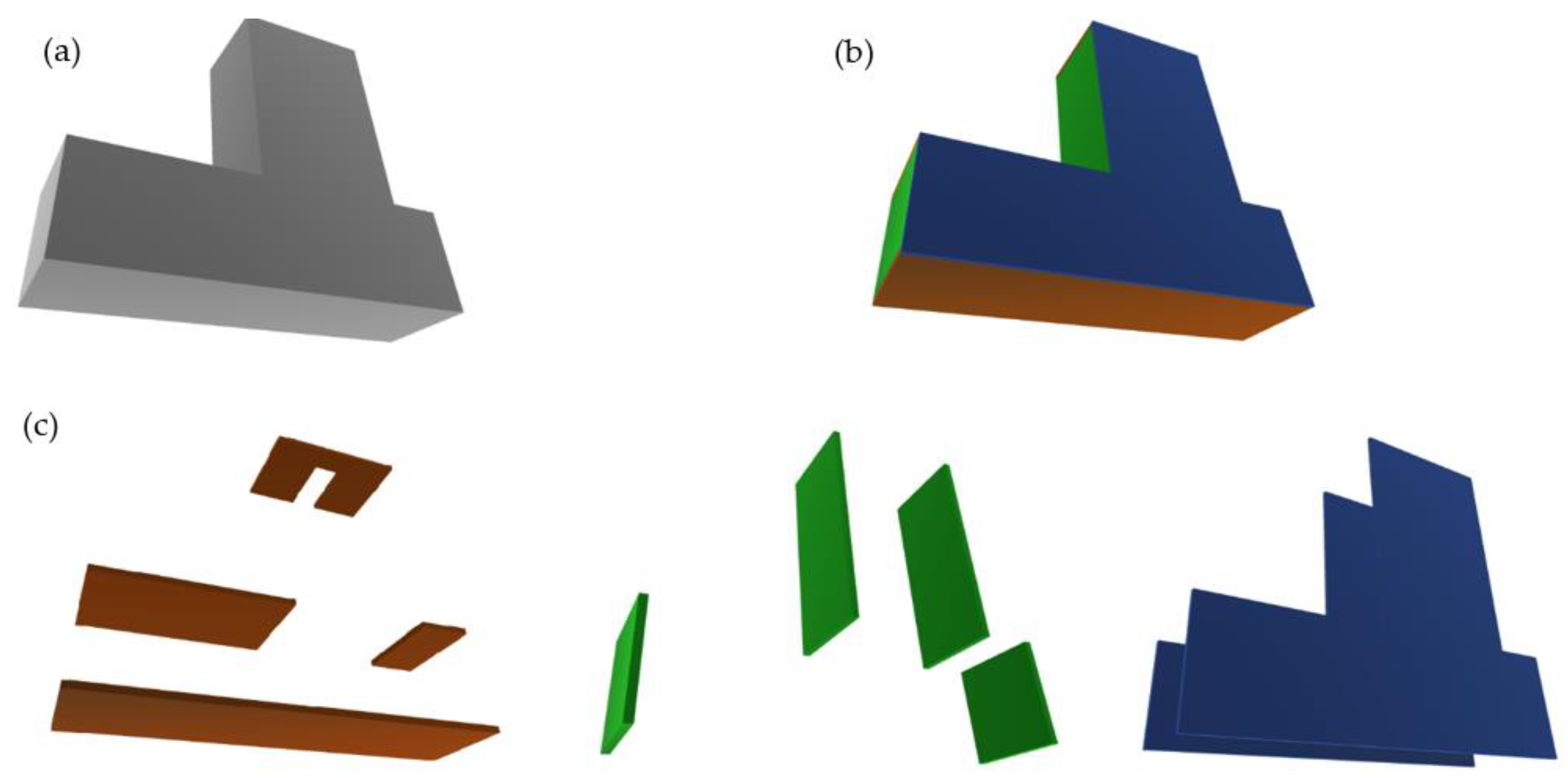
Calculating the direction of clustered plane segments in both the as-planned and as-built models involves two steps, as shown in Figure 2. In the first step, the model, represented by Figure 3a, is segmented to extract all of its plane segments (Figure 3b), which are then clustered based on their orientation in the second step (Figure 3c). The similar normal values of the plane segments in each cluster act as the directions of the model.

3.2.1. Planar Segmentation

The as-built point cloud is first segmented into planar segments with 3D points (x,y,z) and normal vector n(a,b,c) at a distance ‘d’ from the origin satisfying the plane equation: a x + b y + c z + d = 0 . During the segmentation, coplanar segments are handled as one large segment. For extracting the plane structures in the as-planned model, the meshes are split based on their face connectivity.
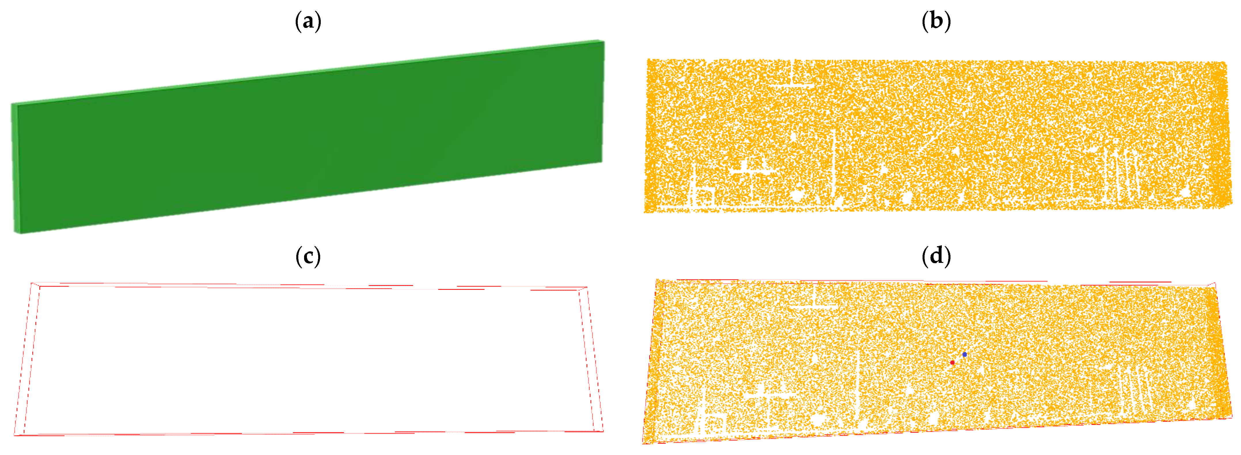
The as-built point cloud may include outliers and occlusions due to the presence of objects in the scene during scanning. On the one hand, to reject outliers, the plane segments are ordered in a hierarchy based on their surface area, where the largest plane segment is ranked first. Only the dominant planes in both models are retained by rejecting the smaller segments based on the suitable threshold expressed as a certain percentage of the area of the largest plane. On the other hand, occlusions have an effect on the determination of the plane centroids, which will be used for calculating the translations in a later stage. For example, the surface coverage of matching plane segments from the as-planned and as-built models, as shown in Figure 4a,b, respectively, are slightly different due to the occlusions in the as-built point cloud. This problem is mitigated by creating an axis-aligned bounding box of each plane segment in the as-built and the BIMs, thus allowing the similar representation of the geometrical shapes in both models (Figure 4a,b). The example in Figure 4c shows the bounding box created from the occluded plane segment (Figure 4b). The centroid calculated from the bounding box is located closer to the center; hence, it is more accurate than the centroid calculated from the occluded point cloud (Figure 4d).

3.2.2. Clustering the Plane Segments

After extracting all the plane segments and determining their geometrical parameters, parallel planes are grouped together into clusters based on their normal vectors. To avoid the failure of the clustering process caused by inaccuracies in the segmentation, a suitable tolerance is introduced in the direction of the normal vectors. The direction of a cluster is defined as the weighted average of the normal vectors according to Equation (1):
n g = i = 1 t n i s i i = 1 t s i
In Equation (1), n g is the weighted normal of a cluster of parallel plane segments, n i represents the normal vector of each segment, s i is the area of the plane segment i , and t is the total number of parallel segments in the cluster.

3.3. Calculating the Possible Rotation Matrices

The rotation matrix is calculated from the directions of the plane clusters in both models. First, all the possible combinations of the three plane cluster directions in both models (as-built and as-planned) are made and the angles between the cluster directions in each combination are calculated. Then, for each combination in the as-built model, these angles are compared to all possible combinations within the as-planned model. Combinations with the same angles are withheld. While comparing the angles, a suitable tolerance is applied to account for slight inaccuracies in the directions. Figure 5a demonstrates an example of a combination with corresponding cluster directions in both models having the same angles.
In the next step, for the combinations that were withheld previously, the rotation matrices are determined in two phases. First, the first pair of normal vectors of the as-built and the as-planned models, as shown in Figure 5b, are aligned with each other by rotating the normal vector of the as-built model around the perpendicular axis, as shown in Figure 5c. Then, the other normal vectors of the as-built model are simultaneously aligned with their corresponding normal vectors by rotating them about the axis defined by the first rotated normal vector, as shown in Figure 5d. The rotation is performed by the Rodriquez rotation formula, given in Equation (2), with an input of the axis of rotation (k) and angle ( θ ) , given in Equation (3).
R ( k ,   θ ) = I + k   sin θ + k 2 ( 1 cos θ )
k   (   k x ,   k y ,   k z ) = [ 0 k z k y k z 0 k x k y k x 0 ]
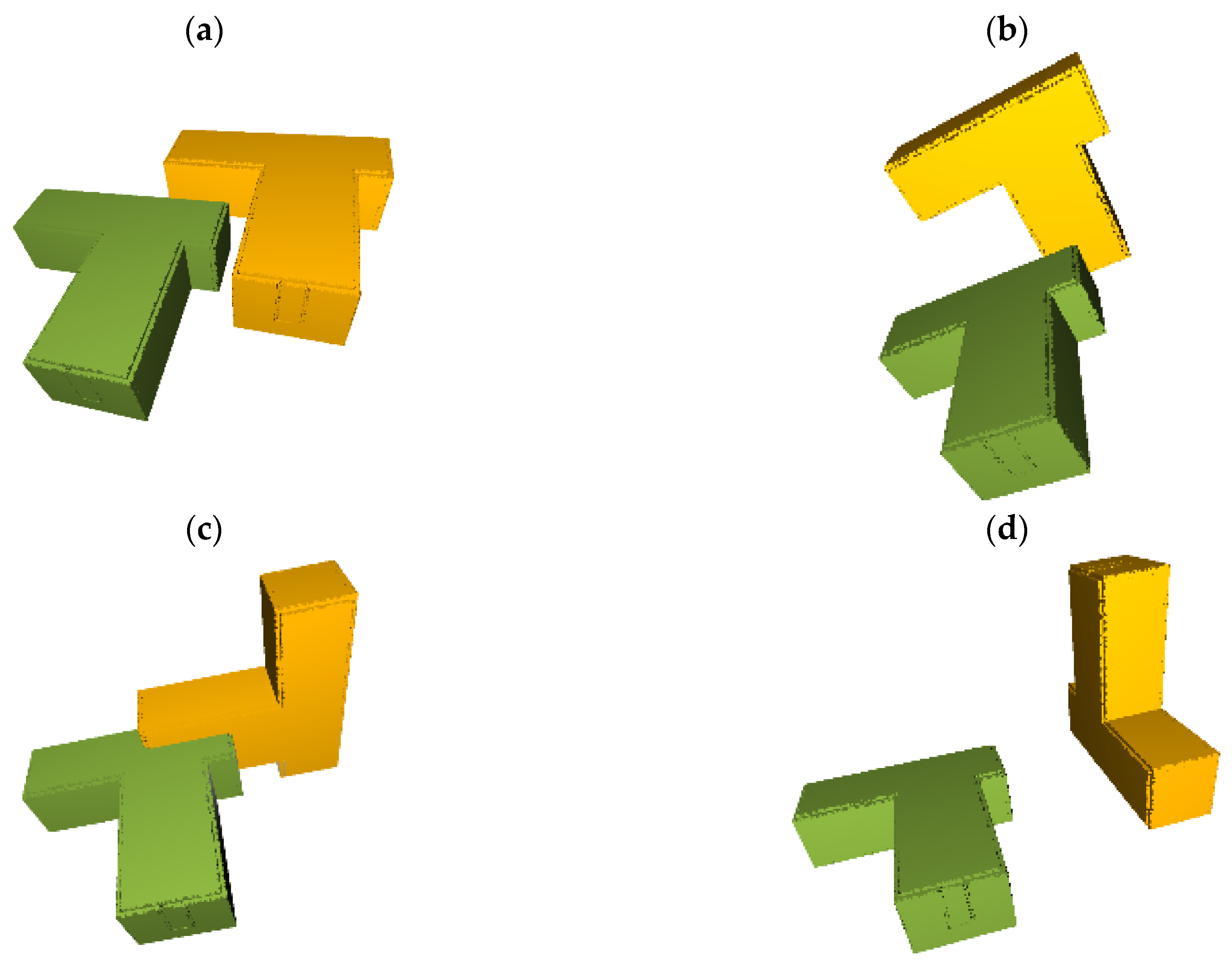
In the case of the occurrence of corresponding combinations with unique angles between their cluster directions, these clusters can automatically be regarded as being the clusters with matching plane segments. In this ideal scenario, the rotation matrix calculated from these corresponding clusters represents the correct orientation of the as-built model with the as-planned model. However, this ideal scenario seldom occurs, as most buildings have an orthogonal geometry with many parallel structural components. This reduces the number of possible distinct angles between plane clusters; hence, the number of possible rotation matrices ( R 1 ,   R 2 ,   ,   R r ) increases substantially. Some rotations resulting from different combinations of the directions of the two models are shown in Figure 6.

3.4. Identifying the Most Likely Rotation Matrix and Translation Vector

Only one of the calculated rotation matrices will lead to the correct orientation of the as-built to the as-planned model. To identify this most likely rotation matrix (and translation vector), a computational framework is proposed here based on the principles that if two models with a similar geometric structure are correctly oriented then:
  • Matching plane segments between the two models should be parallel to each other.
  • The translation between the models should be the same for all matching planar segments.
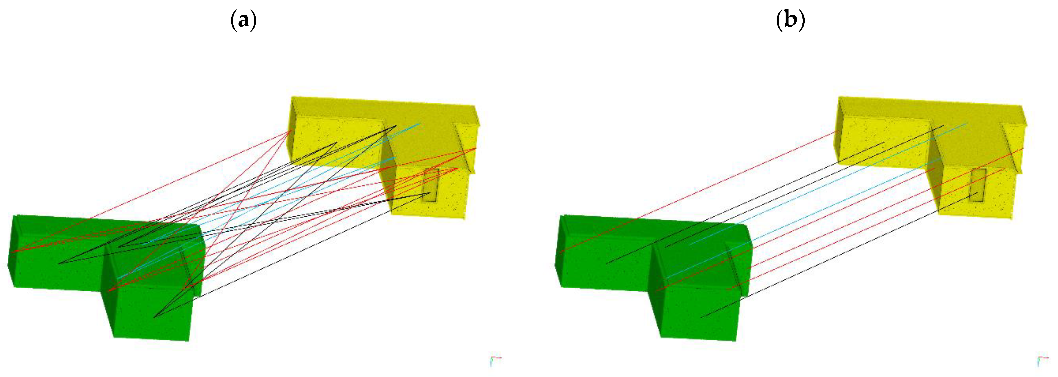
Figure 7 shows a few examples with different orientations of the as-built model relative to the as-planned model to depict how the direction and translation between the matching plane segments can be different if the models are not correctly aligned. Based on this, all the possible rotation matrices are evaluated to identify the rotation matrix offering the most likely alignment. The identification process is performed by assessing the individual plane segments of both models based on their directions and translations for each rotation matrix by computing a matching cost. The details of this calculation are explained below.
For each rotation matrix, first a preliminary assessment of the directions of the plane segments from both models is performed to either discard the rotation matrix, because it is an unlikely candidate, or to continue by computing the total matching cost based on potential matching planes. The assessment workflow is shown in Figure 8.

3.4.1. Directional Assessment

For each rotation matrix, all the plane segments from the as-built model are rotated, after which each rotated plane segment is paired with all the as-planned plane segments. For each pair, the angle between the planes is computed using their normal vector. Pairs of plane segments that are not parallel to each other are rejected, leaving only those pairs with parallel plane segments. If for the majority of the as-built plane segments no parallel plane segments from the as-planned model are found, it is obvious that this particular rotation matrix must be rejected from the list of possible matrices. If, on the other hand, the majority of as-built plane segments have several parallel plane segments in the as-planned model, then the rotation matrix is further scrutinized by considering the pairs of parallel plane segments in the corresponding models as the potential matching plane segments. By lowering the number of rotation matrices based on the directional scrutiny of plane segments, the overall computation time is reduced substantially.

3.4.2. Translational Assessment

Once a rotation matrix is accepted, a matching cost that combines the rotation with the most likely translation is computed. For a particular rotation matrix R, all possible translation vectors t R i , j that map a centroid of a plane segment ‘i’ of the as-built model onto the centroid of a plane segment ‘j’ of the as-planned model are considered. Let C i   and   C j denote the centroids of these planes calculated from their bounding boxes earlier in stage 1. Provided the two planes are almost parallel after rotation, the translation vector t R i , j for this pair is defined as:
t R i , j = C j R C i
The translation vectors determined between all the potential pairs of matching planes for dataset 1 are shown in Figure 9a. From this set of all possible translation vectors, the most likely translations are selected, as shown in Figure 9b. Because of noise in the as-built point cloud, the occlusions in some of the as-built plane segments, and small errors in the alignment, plane segments that are supposed to match may still define slightly different translations. Therefore, a minimization process is proposed by allocating a cost to each possible translation vector, which takes into account that some segments may be incomplete or not aligned correctly.
Depending on the translation, each plane segment from the as-built model may have more than one potential matching plane from the as-planned model. Therefore, the assumption is made that the most likely match is the one for which the distance between the centroids is minimal. Let t R o denote a possible translation and R represent one of the rotation matrices. For a particular plane segment ‘i’ from the as-built model, the most likely matching plane segment of the as-planned model is then j = argmin j | | t R o t R i , j | | . That is, from all possible translation vectors that map the centroid of segment ‘i’ onto one of the centroids of the as-planned model, the one closest to the proposed translation t R o is chosen. The total matching cost, as a function of t R o and R, is then defined as:
σ   ( t R o ) = i = 1 m ( min j | | t R o t R i , j | | 2 ) m
The most likely translation t R o for rotation matrix R is found by minimizing the above total matching cost over a finite set of translation vectors. To further simplify the computation, it is also assumed that the optimal translation vector t R o will be close to one of the translation vectors t R i , j :
t R o t R p , q   :       ( p , q ) = argmin ( i , j ) σ ( t R i , j )
Similarly, the most likely rotation matrix R o is also identified from a finite set of pre-filtered rotation matrices.
R o = argmin R σ ( t R o )       R     { R 1 ,   R 2 ,   R 3 ,   R r }
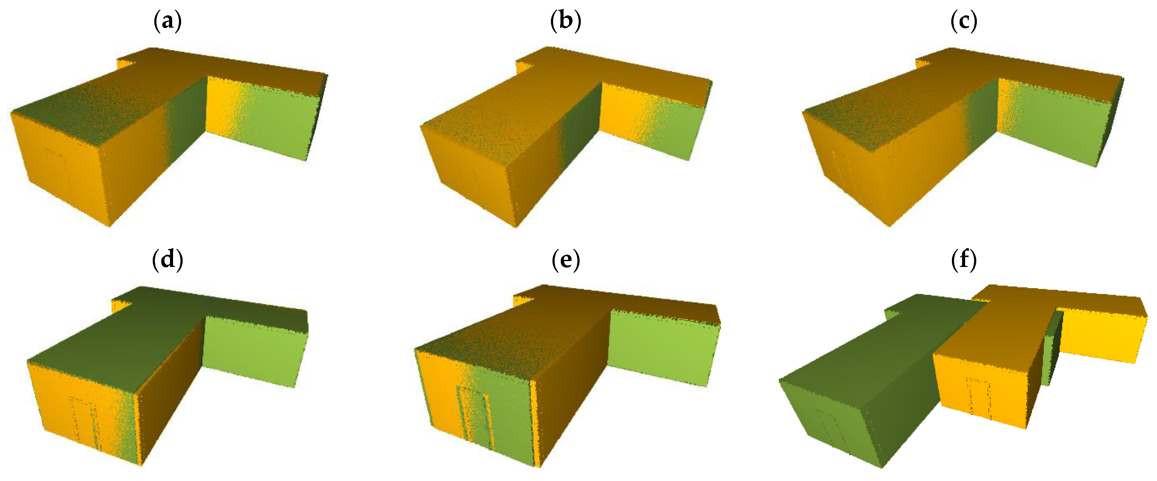
Hence, the matching cost ensures that the most likely rotation matrix, as compared to other matrices, is measuring the matching of all the corresponding plane segments of both models, as shown in Figure 10. Similarly, it also confirms the most likely translation is determined from the potential pair of matching plane segments that is offering the maximum overlap of all the matching plane segments, as shown in Figure 11. To further improve the registration, fine registration using ICP can be performed in the end, if required.

4. Results

The proposed method was validated by tests on different datasets, including both simulated and real-life datasets that were different from each other in terms of their architectural shape, the number of planes, and the number of 3D points in their as-built model. The simulated data were used to validate the theoretical framework, while the real-life datasets helped in understanding the practical difficulties and limitations of the proposed method in real building projects.
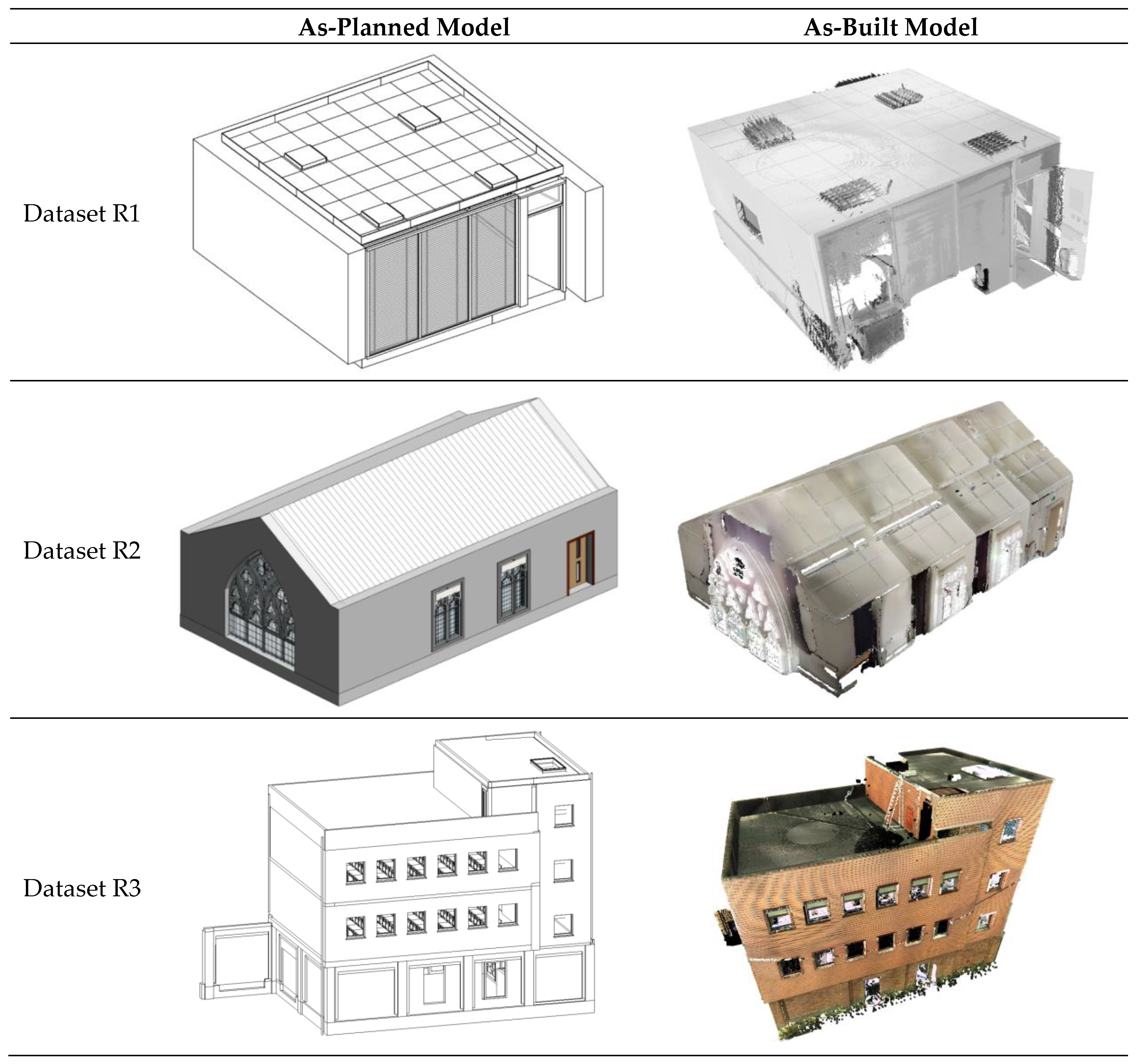
For the simulated datasets (S1, S2, and S3), the as-built model was derived from the as-planned model with random transformation. The registration of the as-built model with its original model allowed us to analyze the proposed method without any influence of factors including noise, outliers, or missing information. The real-life case studies (datasets R1, R2, and R3) were carried out to test the validity of the proposed method using laser scan data for the as-built model together with the BIM model of the same existing building. The geometric details of all the datasets are presented in Table 1, and the real-life datasets R1, R2, and R3 are shown in more detail in Figure 12. The dataset R3 was used in [75,76] as well.
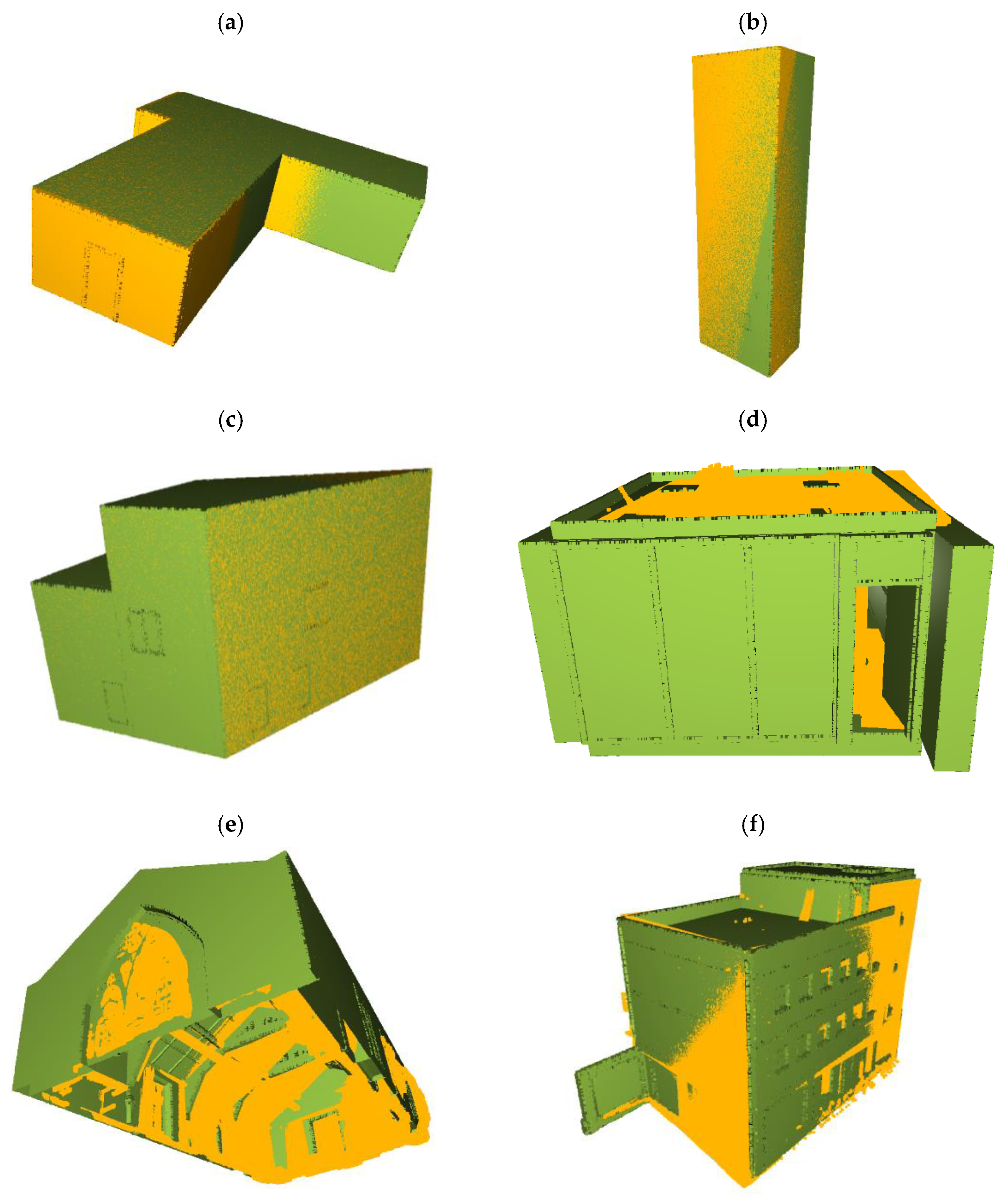
All the datasets, both stimulated and real, were successfully registered using the proposed method. Figure 13 shows the registration results for all the datasets, while the respective processing details of the registration are listed in Table 2. To increase the reliability of the results in relation to processing time and accuracy, each dataset was processed at least 100 times and the average values were considered for the evaluation. The reported results were obtained by initially down-sampling the as-built cloud points during preprocessing using a voxel size of 0.2 m. Similarly, plane segmentation was performed using RANSAC with the number of iterations limited to 3000. Furthermore, because the directions of the plane segments can be slightly faulty due to the presence of noise in the point cloud, a suitable tolerance level according to the datasets was set for the normal values of plane segments during the process of clustering to determine the directions of clustered plane segments. All the processing was conducted on a laptop with an Intel i7-8850H CPU with 16 GB RAM and the proposed method was implemented in the Python language. The proposed method was further analyzed in terms of processing time and accuracy to evaluate its performance and explore its limitations.

5. Discussion

5.1. Time Efficiency

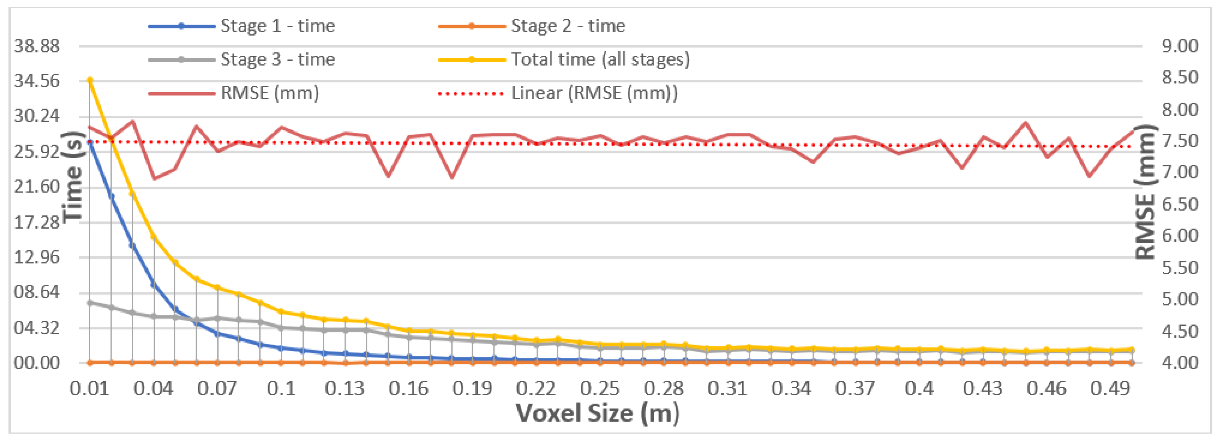
The time efficiency of the proposed technique was analyzed in detail. First, the effect of voxel size on processing time was examined. Generally, a decrease in voxel size increased the size of the point cloud, which in turn increased the processing time. However, an increase in voxel size induces a loss of detail, leading to a possible decrease in the registration accuracy. Hence, a compromise must be found. Therefore, the processing time of the different processing stages (illustrated in Figure 1), as well as the overall registration accuracy, were analyzed with a range of different voxel sizes for dataset S1. The results are shown in Figure 14, where it can be observed that the overall processing time of the method significantly increased once the voxel size was lowered to 0.1m. The time complexity of the proposed technique is O ( log n ) ,   where   n equals the voxel size in a grid. When the computation time was analyzed per processing stage, it was clear that the overall processing time was not affected by stage 2, while the processing time of stage 3 increased approximately linearly with a decreasing voxel size, and the computation time in stage 1 increased significantly once the voxel size dropped under 0.1 m. This major increment in computation can be attributed to the plane segmentation of the as-built point cloud that is performed using RANSAC segmentation, which estimates the plane from the voxelized points in numerous iterations. Therefore, the voxel size should be chosen to be between 0.1 m and 0.5 m to ensure the success of the proposed method and limit the significant increment in processing time.
To gain insight into the influence of different parameters on the computation time, the overall processing time of all the datasets was further analyzed at a voxel size of 0.2 m, as shown in Table 3. As could be expected, the total number of plane segments was the determining factor influencing the processing time in stages one and three.
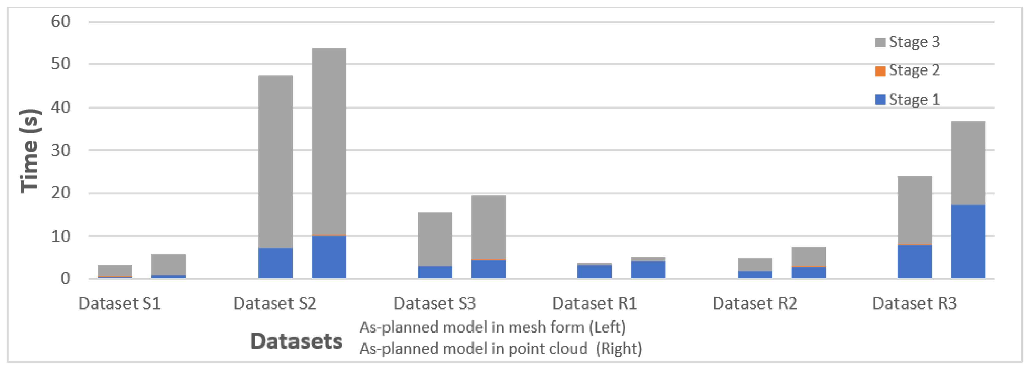
As the proposed method processes the as-planned model from the BIM directly into the triangulated mesh instead of the point cloud, the total processing time of the proposed technique was also analyzed by processing the as-planned model in both triangulated mesh and point cloud form. It was found that extracting the geometric parameters directly from the triangulated mesh of the as-planned model instead of converting it into a point cloud had a positive impact on the overall computation time, as shown in Figure 15. This is due to the fact that the required plane parameters (such as the normal of a plane) can be extracted directly from the mesh model, while in the case of the point cloud, these parameters are calculated from the 3D points of plane segments, which increases the processing time.

5.2. Registration Accuracy

The accuracy of the proposed method was evaluated by comparing the transformed as-built model to the ground truth model. The ground truth model is the as-planned model and the fine registered as-built model for stimulated and real-life datasets, respectively. According to Figure 14, the voxel size did not the registration accuracy in terms of RMSE. As the root mean square error (RMSE) is not only an effective indicator of registration accuracy [34], the rotation error (in degrees) and translation error (in mm) for each dataset were also calculated, using Equations (8) and (9), respectively.
ϵ R = | θ G T θ T |
ϵ t = | | t G T t T | |
In Equation (8), θ G T and θ T denote the quaternion rotation angles of the ground truth and the transformed model, respectively, whereas t G T and t T represent the translation vectors of the ground truth and the transformed model, respectively, in Equation (9). The results of the evaluation metrics are listed in Table 3; they indicate a good accuracy of the proposed method. From the results, it is evident that building structures with an overall simple geometry and fewer planes had relatively higher accuracy. The accuracy in terms of rotation was high in all datasets. This is inherent to the proposed method due to the accurate normal values of plane segments. The normal values of plane segments obtained from the mesh surfaces in the as-planned model are error-free, and the normal values from the as-built model are determined through RANSAC plane estimation with a high iteration value. Furthermore, the proposed method computes the weighted average for parallel segments to ensure a minimal influence of inaccurately extracted normal values, if any.
It should be noted that the proposed method depends on plane segments extracted randomly from the as-built model by means of RANSAC plane estimation, and the registration parameters may change slightly each time the proposed method is applied, thus also slightly impacting the resulting registration accuracy. However, these minor changes can be covered by fine registration through an ICP algorithm, if required.

5.3. Effect of Noise and Occlusion

The effect of noise on the success ratio along with different voxel sizes was also analyzed. It was observed that the voxel size influenced the planar segmentation stage in the proposed method, as a greater voxel size decreased the number of 3D points in the model. If the amount of 3D points is too low, the planar segmentation may extract inaccurate plane segments from the model, which affects the results of the proposed technique. The presence of noise in the point cloud may hinder the detection of plane segments, thus also attributing to the possible failure of the proposed technique, although this can be solved by decreasing the voxel size. Table 4 illustrates different point cloud models of dataset 1 having Gaussian noise with a variance of zero and a standard deviation ranging from 0 to 0.15. Planar segmentation was performed on these point clouds after down-sampling them with voxel sizes from 0.01 to 0.37 m. It was evident that a higher voxel size enabled the extraction of accurate plane segments, even in the presence of strong noise, for the success of the proposed method.

5.4. Application on Partially Constructed Buildings

To investigate the registration success of partially constructed as-built models with their as-planned model for automated construction progress monitoring, the proposed method was evaluated using as-built models with different combinations of missing planes simulating different stages of completion. During testing, it was found that the proposed method worked successfully if the necessary conditions were met. These conditions include: (i) as-built models with an overall unsymmetrical structure should have at least three planes in distinct directions and (ii) the size of most plane segments should correspond highly to their conjugate segments in the as-planned model. The presence of at least three planes in distinct directions assures that the correct rotation matrix will be calculated in the second stage along with other possible rotation matrices. Similarly, conjugate plane segments with high geometrical correspondence improve the identification of matching plane segments in the third stage.
Generally, the building models met these two conditions, and even a scan of a small typical building had plane segments in three distinct directions with a point cloud covering the walls for the most part. In the worst scenario, with a major missing part in the point clouds, the registration can further be improved through ICP registration. Figure 16 shows an example of a modified simulated model of dataset 1 with an as-planned model (Figure 16a) and an as-built model (Figure 16b) with just three plane segments that were successfully registered through the proposed method. In this example, all three plane segments of the as-planned model had different directions and were identical in size to their corresponding segments. Similarly, it is also evident that the proposed method accurately calculated the translation based on matching planes even if the major part of the model was missing, as compared to the traditional technique based on the centroid of whole models, as shown in Figure 16c,d.

6. Conclusions

Construction project monitoring includes the registration of as-built models with their as-planned model followed by the analysis of the aligned models to infer progress information. Normally, the registration process involves two steps: (1) coarse registration, in which both models are almost aligned to each other, and (2) fine registration, which involves an improvement of the coarse registration and augments the registration accuracy. This research addressed the coarse registration problem in detail and proposed a new automated method to align the as-built and as-planned building models using their geometric features in a highly robust and accurate way. Most building structures have an orthogonal geometry that consists primarily of plane segments. The extraction of these planar features is only slightly affected by the presence of noise or minor outliers; therefore, the proposed technique employs these features for the automated registration of building models for project monitoring. The technique first utilizes the directions of the planes from the building models to determine the possible rotations for the registration. Then, it measures the matching between all the plane segments to recognize the rotation with the best match. Consequently, the translation is calculated from the best-matched plane segments. Along with the transformation parameters, the proposed method also has the ability to identify the matching plane segments between corresponding models. The identification of plane segments, representing the building components, can further aid in their individual inspection during project monitoring.
Experimentation was performed on building datasets with different geometries to evaluate the performance of the proposed method. The results demonstrated that the proposed method successfully registered all the building models with a high rotation and translation accuracy in a fully automated way. The presence of noise or occlusions only slightly affected the success of registration. The proposed method also proved to be robust in terms of computation time; however, the processing time was highly dependent on the number of plane segments.
Overall, the proposed method exhibits reliable results for both complete and incomplete buildings, which makes it useful for progress monitoring as long as at least three identical plane segments with distinct directions are present in both models. From the perspective of construction management, the automated registration of scan models of partially completed as-built situations with their BIM model is a big step forward in the development of an automated system for project monitoring. Further research is necessary to enhance the applicability of the proposed method in complex buildings with a high number of planes and/or curved elements.

Author Contributions

Conceptualization, N.A.S. and P.V.; methodology, N.A.S. and P.V.; validation, N.A.S.; formal analysis, N.A.S.; data curation, N.A.S.; writing—original draft preparation, N.A.S.; writing—review and editing, G.D. and P.V.; supervision, G.D. and P.V. All authors have read and agreed to the published version of the manuscript.

Funding

This research received no external funding.

Acknowledgments

We would like to thank Shawn O’Keeffe from BIM & Scan and Maarten Bassier from KU Leuven for providing the datasets.

Conflicts of Interest

The authors declare no conflict of interest.

References

  1. Bosché, F. Automated recognition of 3D CAD model objects in laser scans and calculation of as-built dimensions for dimensional compliance control in construction. Adv. Eng. Inform. 2010, 24, 107–118. [Google Scholar] [CrossRef]
  2. Navon, R. Research in automated measurement of project performance indicators. Autom. Constr. 2007, 16, 176–188. [Google Scholar] [CrossRef]
  3. Zhang, X.; Bakis, N.; Lukins, T.C.; Ibrahim, Y.M.; Wu, S.; Kagioglou, M.; Aouad, G.; Kaka, A.P.; Trucco, E. Automating progress measurement of construction projects. Autom. Constr. 2009, 18, 294–301. [Google Scholar] [CrossRef]
  4. Han, K.K.; Golparvar-Fard, M. Automated monitoring of operation-level construction progress using 4D BIM and daily site photologs. In Proceedings of the Construction Research Congress 2014: Construction in a Global Network, Atlanta, GA, USA, 19–21 May 2014; pp. 1033–1042. [Google Scholar]
  5. Omar, T.; Nehdi, M.L. Automated Data Collection for Progress Tracking Purposes: A Review of Related Techniques. In Proceedings of the International Congress and Exhibition “Sustainable Civil Infrastructures: Innovative Infrastructure Geotechnology”, Sharm El Sheikh, Egypt, 15–20 July 2017; pp. 391–405. [Google Scholar]
  6. Fang, J.; Li, Y.; Liao, Q.; Ren, Z.; Xie, B. Construction Progress Control And Management Measures Analysis. Smart Constr. Res. 2018, 2. [Google Scholar] [CrossRef]
  7. Golparvar-Fard, M.; Savarese, S.; Peña-Mora, F. Interactive Visual Construction Progress Monitoring with D4 AR—4D Augmented Reality—Models. In Proceedings of the Construction Research Congress 2009: Building a Sustainable Future, Seattle, WA, USA, 5–7 April 2009; pp. 41–50. [Google Scholar]
  8. Braun, A.; Tuttas, S.; Borrmann, A.; Stilla, U. A concept for automated construction progress monitoring using BIM-based geometric constraints and photogrammetric point clouds. J. Inf. Technol. Constr. (ITcon) 2015, 20, 68–79. [Google Scholar]
  9. Omar, H.; Dulaimi, M. Using BIM to automate construction site activities. Build. Inf. Model. (BIM) Des. Constr. Oper. 2015, 149, 45. [Google Scholar]
  10. Pučko, Z.; Šuman, N.; Rebolj, D. Automated continuous construction progress monitoring using multiple workplace real time 3D scans. Adv. Eng. Inform. 2018, 38, 27–40. [Google Scholar] [CrossRef]
  11. Rebolj, D.; Pučko, Z.; Babič, N.Č.; Bizjak, M.; Mongus, D. Point cloud quality requirements for Scan-vs-BIM based automated construction progress monitoring. Autom. Constr. 2017, 84, 323–334. [Google Scholar] [CrossRef]
  12. Khairadeen Ali, A.; Lee, O.J.; Lee, D.; Park, C. Remote Indoor Construction Progress Monitoring Using Extended Reality. Sustainability 2021, 13, 2290. [Google Scholar] [CrossRef]
  13. Fathi, H.; Dai, F.; Lourakis, M. Automated as-built 3D reconstruction of civil infrastructure using computer vision: Achievements, opportunities, and challenges. Adv. Eng. Inform. 2015, 29, 149–161. [Google Scholar] [CrossRef]
  14. Golparvar-Fard, M.; Pena-Mora, F.; Savarese, S. Monitoring changes of 3D building elements from unordered photo collections. In Proceedings of the Computer Vision Workshops (ICCV Workshops), 2011 IEEE International Conference, Barcelona, Spain, 6–13 November 2011; pp. 249–256. [Google Scholar]
  15. Golparvar-Fard, M.; Peña-Mora, F.; Savarese, S. Automated progress monitoring using unordered daily construction photographs and IFC-based building information models. J. Comput. Civil. Eng. 2012, 29, 04014025. [Google Scholar] [CrossRef]
  16. Han, K.; Degol, J.; Golparvar-Fard, M. Geometry-and Appearance-Based Reasoning of Construction Progress Monitoring. J. Constr. Eng. Manag. 2017, 144, 04017110. [Google Scholar] [CrossRef] [Green Version]
  17. Tuttas, S.; Braun, A.; Borrmann, A.; Stilla, U. Acquisition and consecutive registration of photogrammetric point clouds for construction progress monitoring using a 4D BIM. PFG–J. Photogramm. Remote Sens. Geoinf. Sci. 2017, 85, 3–15. [Google Scholar] [CrossRef]
  18. Bosche, F.; Haas, C.T. Automated retrieval of 3D CAD model objects in construction range images. Autom. Constr. 2008, 17, 499–512. [Google Scholar] [CrossRef]
  19. Kim, C.; Son, H.; Kim, C. Automated construction progress measurement using a 4D building information model and 3D data. Autom. Constr. 2013, 31, 75–82. [Google Scholar] [CrossRef]
  20. Tang, P.; Huber, D.; Akinci, B.; Lipman, R.; Lytle, A. Automatic reconstruction of as-built building information models from laser-scanned point clouds: A review of related techniques. Autom. Constr. 2010, 19, 829–843. [Google Scholar] [CrossRef]
  21. Turkan, Y.; Bosche, F.; Haas, C.T.; Haas, R. Automated progress tracking using 4D schedule and 3D sensing technologies. Autom. Constr. 2012, 22, 414–421. [Google Scholar] [CrossRef]
  22. Brilakis, I.; Lourakis, M.; Sacks, R.; Savarese, S.; Christodoulou, S.; Teizer, J.; Makhmalbaf, A. Toward automated generation of parametric BIMs based on hybrid video and laser scanning data. Adv. Eng. Inform. 2010, 24, 456–465. [Google Scholar] [CrossRef]
  23. El-Omari, S.; Moselhi, O. Integrating 3D laser scanning and photogrammetry for progress measurement of construction work. Autom. Constr. 2008, 18, 1–9. [Google Scholar] [CrossRef]
  24. Shahi, A.; Aryan, A.; West, J.S.; Haas, C.T.; Haas, R.C. Deterioration of UWB positioning during construction. Autom. Constr. 2012, 24, 72–80. [Google Scholar] [CrossRef]
  25. Besl, P.J.; McKay, N.D. Method for registration of 3-D shapes. In Proceedings of the Sensor Fusion IV: Control Paradigms and Data Structures, Boston, MA, USA, 12–15 November 1991; pp. 586–606. [Google Scholar]
  26. Zhang, Z. Iterative point matching for registration of free-form curves and surfaces. Int. J. Comput. Vis. 1994, 13, 119–152. [Google Scholar] [CrossRef]
  27. Chen, Y.; Medioni, G. Object modelling by registration of multiple range images. Image Vis. Comput. 1992, 10, 145–155. [Google Scholar] [CrossRef]
  28. Rusinkiewicz, S.; Levoy, M. Efficient variants of the ICP algorithm. In Proceedings of the International Conference on 3D Digital Imaging and Modeling, Quebec City, QC, Canada, 28 May–1 June 2001. [Google Scholar]
  29. Hattab, A.; Taubin, G. 3D rigid registration of cad point-clouds. In Proceedings of the 2018 International Conference on Computing Sciences and Engineering (ICCSE), Kuwait City, Kuwait, 11–13 March 2018; pp. 1–6. [Google Scholar]
  30. Bueno, M.; Bosché, F.; González-Jorge, H.; Martínez-Sánchez, J.; Arias, P. 4-Plane congruent sets for automatic registration of as-is 3D point clouds with 3D BIM models. Autom. Constr. 2018, 89, 120–134. [Google Scholar] [CrossRef]
  31. Anil, E.B.; Tang, P.; Akinci, B.; Huber, D. Assessment of the quality of as-is building information models generated from point clouds using deviation analysis. In Proceedings of the Three-Dimensional Imaging, Interaction, and Measurement, San Francisco, CA, USA, 24–27 January 2011; p. 78640F. [Google Scholar]
  32. Bassier, M.; Vergauwen, M.; Poux, F. Point Cloud vs. Mesh Features for Building Interior Classification. Remote Sens. 2020, 12, 2224. [Google Scholar] [CrossRef]
  33. Li, J.; Hu, Q.; Ai, M. GESAC: Robust graph enhanced sample consensus for point cloud registration. ISPRS J. Photogramm. Remote Sens. 2020, 167, 363–374. [Google Scholar] [CrossRef]
  34. Zong, W.; Li, M.; Zhou, Y.; Wang, L.; Xiang, F.; Li, G. A Fast and Accurate Planar-Feature-Based Global Scan Registration Method. IEEE Sens. J. 2019, 19, 12333–12345. [Google Scholar] [CrossRef]
  35. Xu, Y.; Boerner, R.; Yao, W.; Hoegner, L.; Stilla, U. Automated Coarse Registration of Point Clouds in 3D Urban Scenes Using voxel based plane constraint. ISPRS Ann. Photogramm. Remote Sens. Spat. Inf. Sci. 2017, 4, 185. [Google Scholar] [CrossRef] [Green Version]
  36. Bolles, R.C.; Fischler, M.A. A RANSAC-based approach to model fitting and its application to finding cylinders in range data. In Proceedings of the IJCAI, Vancouver, BC, Canada, 24–28 August 1981; pp. 637–643. [Google Scholar]
  37. Chen, C.-S.; Hung, Y.-P.; Cheng, J.-B. RANSAC-based DARCES: A new approach to fast automatic registration of partially overlapping range images. IEEE Trans. Pattern Anal. Mach. Intell. 1999, 21, 1229–1234. [Google Scholar] [CrossRef] [Green Version]
  38. Fontanelli, D.; Ricciato, L.; Soatto, S. A fast ransac-based registration algorithm for accurate localization in unknown environments using lidar measurements. In Proceedings of the 2007 IEEE International Conference on Automation Science and Engineering, Xi’an, China, 22–25 September 2007; pp. 597–602. [Google Scholar]
  39. Theiler, P.W.; Wegner, J.D.; Schindler, K. Keypoint-based 4-points congruent sets–automated marker-less registration of laser scans. ISPRS J. Photogramm. Remote Sens. 2014, 96, 149–163. [Google Scholar] [CrossRef]
  40. Mellado, N.; Aiger, D.; Mitra, N.J. Super 4pcs fast global pointcloud registration via smart indexing. In Computer Graphics Forum; Wiley: Hoboken, NJ, USA, 2014; Volume 33, pp. 205–215. 4p. [Google Scholar]
  41. Aiger, D.; Mitra, N.J.; Cohen-Or, D. 4-points congruent sets for robust pairwise surface registration. In ACM SIGGRAPH 2008 Papers; ACM: New York, NY, USA, 2008; pp. 1–10. [Google Scholar]
  42. Xu, Y.; Boerner, R.; Yao, W.; Hoegner, L.; Stilla, U. Pairwise coarse registration of point clouds in urban scenes using voxel-based 4-planes congruent sets. ISPRS J. Photogramm. Remote Sens. 2019, 151, 106–123. [Google Scholar] [CrossRef]
  43. Böhm, J.; Becker, S. Automatic marker-free registration of terrestrial laser scans using reflectance. In Proceedings of the 8th Conference on Optical 3D Measurement Techniques, Zurich, Switzerland, 9–12 July 2007; pp. 9–12. [Google Scholar]
  44. Weinmann, M.; Weinmann, M.; Hinz, S.; Jutzi, B. Fast and automatic image-based registration of TLS data. ISPRS J. Photogramm. Remote Sens. 2011, 66, S62–S70. [Google Scholar] [CrossRef]
  45. Theiler, P.; Schindler, K. Automatic registration of terrestrial laser scanner point clouds using natural planar surfaces. ISPRS Ann. Photogramm. Remote Sens. Spat. Inf. Sci. 2012, 3, 173–178. [Google Scholar] [CrossRef] [Green Version]
  46. Weber, T.; Hänsch, R.; Hellwich, O. Automatic registration of unordered point clouds acquired by Kinect sensors using an overlap heuristic. ISPRS J. Photogramm. Remote Sens. 2015, 102, 96–109. [Google Scholar] [CrossRef]
  47. Yang, B.; Dong, Z.; Liang, F.; Liu, Y. Automatic registration of large-scale urban scene point clouds based on semantic feature points. ISPRS J. Photogramm. Remote Sens. 2016, 113, 43–58. [Google Scholar] [CrossRef]
  48. Mahmood, B.; Han, S.; Lee, D.-E. BIM-Based Registration and Localization of 3D Point Clouds of Indoor Scenes Using Geometric Features for Augmented Reality. Remote Sens. 2020, 12, 2302. [Google Scholar] [CrossRef]
  49. Li, Z.; Zhang, X.; Tan, J.; Liu, H. Pairwise Coarse Registration of Indoor Point Clouds Using 2D Line Features. ISPRS Int. J. Geo-Inf. 2021, 10, 26. [Google Scholar] [CrossRef]
  50. Habib, A.; Ghanma, M.; Morgan, M.; Al-Ruzouq, R. Photogrammetric and LiDAR data registration using linear features. Photogramm. Eng. Remote Sens. 2005, 71, 699–707. [Google Scholar] [CrossRef]
  51. Al-Durgham, M.; Habib, A. A framework for the registration and segmentation of heterogeneous LiDAR data. Photogrammetric Eng. Remote Sens. 2013, 79, 135–145. [Google Scholar] [CrossRef]
  52. Yang, B.; Zang, Y. Automated registration of dense terrestrial laser-scanning point clouds using curves. ISPRS J. Photogramm. Remote Sens. 2014, 95, 109–121. [Google Scholar] [CrossRef]
  53. Xiao, J.; Adler, B.; Zhang, J.; Zhang, H. Planar segment based three-dimensional point cloud registration in outdoor environments. J. Field Robot. 2013, 30, 552–582. [Google Scholar] [CrossRef]
  54. Dold, C.; Brenner, C. Registration of terrestrial laser scanning data using planar patches and image data. Int. Arch. Photogramm. Remote Sens. Spat. Inf. Sci.-ISPRS Arch. 2006, 36, 78–83. [Google Scholar]
  55. Ge, X.; Wunderlich, T. Surface-based matching of 3D point clouds with variable coordinates in source and target system. ISPRS J. Photogramm. Remote Sens. 2016, 111, 1–12. [Google Scholar] [CrossRef] [Green Version]
  56. Xu, Y.; Hoegner, L.; Tuttas, S.; Stilla, U. Voxel-and Graph-based point cloud segmentation of 3d scenes using perceptual grouping laws. ISPRS Ann. Photogramm. Remote Sens. Spat. Inf. Sci. 2017, 4, 43–50. [Google Scholar] [CrossRef] [Green Version]
  57. Pavan, N.L.; dos Santos, D.R.; Khoshelham, K. Global Registration of Terrestrial Laser Scanner Point Clouds Using Plane-to-Plane Correspondences. Remote Sens. 2020, 12, 1127. [Google Scholar] [CrossRef] [Green Version]
  58. Li, L.; Yang, F.; Zhu, H.; Li, D.; Li, Y.; Tang, L. An improved RANSAC for 3D point cloud plane segmentation based on normal distribution transformation cells. Remote Sens. 2017, 9, 433. [Google Scholar] [CrossRef] [Green Version]
  59. Schnabel, R.; Wahl, R.; Klein, R. Efficient RANSAC for point-cloud shape detection. Comput. Graph. Forum 2007, 26, 214–226. [Google Scholar] [CrossRef]
  60. Nurunnabi, A.; Belton, D.; West, G. Robust segmentation in laser scanning 3D point cloud data. In Proceedings of the 2012 International Conference on Digital Image Computing Techniques and Applications (DICTA), Fremantle, Australia, 3–5 December 2012; pp. 1–8. [Google Scholar]
  61. Li, M.; Gao, X.; Wang, L.; Li, G. Automatic registration of laser-scanned point clouds based on planar features. In Proceedings of the 2nd ISPRS International Conference on Computer Vision in Remote Sensing (CVRS 2015), Xiamen, China, 28–30 April 2015; p. 990103. [Google Scholar]
  62. Grant, W.S.; Voorhies, R.C.; Itti, L. Finding planes in LiDAR point clouds for real-time registration. In Proceedings of the 2013 IEEE/RSJ International Conference on Intelligent Robots and Systems, Tokyo, Japan, 3–7 November 2013; pp. 4347–4354. [Google Scholar]
  63. Poppinga, J.; Vaskevicius, N.; Birk, A.; Pathak, K. Fast plane detection and polygonalization in noisy 3D range images. In Proceedings of the 2008 IEEE/RSJ International Conference on Intelligent Robots and Systems, Nice, France, 22–26 September 2008; pp. 3378–3383. [Google Scholar]
  64. Zhang, D.; Huang, T.; Li, G.; Jiang, M. Robust algorithm for registration of building point clouds using planar patches. J. Surv. Eng. 2012, 138, 31–36. [Google Scholar] [CrossRef]
  65. He, W.; Ma, W.; Zha, H. Automatic registration of range images based on correspondence of complete plane patches. In Proceedings of the Fifth International Conference on 3-D Digital Imaging and Modeling (3DIM’05), Ottawa, ON, Canada, 13–16 June 2005; pp. 470–475. [Google Scholar]
  66. Brenner, C.; Dold, C.; Ripperda, N. Coarse orientation of terrestrial laser scans in urban environments. ISPRS J. Photogramm. Remote Sens. 2008, 63, 4–18. [Google Scholar] [CrossRef]
  67. Pavan, N.L.; dos Santos, D.R. A global closed-form refinement for consistent TLS data registration. IEEE Geosci. Remote Sens. Lett. 2017, 14, 1131–1135. [Google Scholar] [CrossRef]
  68. Zhang, C.; Arditi, D. Automated progress control using laser scanning technology. Autom. Constr. 2013, 36, 108–116. [Google Scholar] [CrossRef]
  69. Kim, C.; Son, H.; Kim, C. Fully automated registration of 3D data to a 3D CAD model for project progress monitoring. Autom. Constr. 2013, 35, 587–594. [Google Scholar] [CrossRef]
  70. Liu, Y.-S.; Ramani, K. Robust principal axes determination for point-based shapes using least median of squares. Comput.-Aided Des. 2009, 41, 293–305. [Google Scholar] [CrossRef] [Green Version]
  71. Fitzgibbon, A.W. Robust registration of 2D and 3D point sets. Image Vis. Comput. 2003, 21, 1145–1153. [Google Scholar] [CrossRef]
  72. Chen, J.; Cho, Y.K. Point-to-point comparison method for automated scan-vs-bim deviation detection. In Proceedings of the 17th International Conference on Computing in Civil and Building Engineering, Tampere, Finland, 5–7 June 2018. [Google Scholar]
  73. Wand, M.; Berner, A.; Bokeloh, M.; Jenke, P.; Fleck, A.; Hoffmann, M.; Maier, B.; Staneker, D.; Schilling, A.; Seidel, H.-P. Processing and interactive editing of huge point clouds from 3D scanners. Comput. Graph. 2008, 32, 204–220. [Google Scholar] [CrossRef]
  74. Medioni, G.; Lee, M.-S.; Tang, C.-K. A Computational Framework for Segmentation and Grouping; Elsevier: Amsterdam, The Netherlands, 2000. [Google Scholar]
  75. Bassier, M.; Vergauwen, M. Clustering of wall geometry from unstructured point clouds using conditional random fields. Remote Sens. 2019, 11, 1586. [Google Scholar] [CrossRef] [Green Version]
  76. Bassier, M.; Vergauwen, M. Unsupervised reconstruction of Building Information Modeling wall objects from point cloud data. Autom. Constr. 2020, 120, 103338. [Google Scholar] [CrossRef]
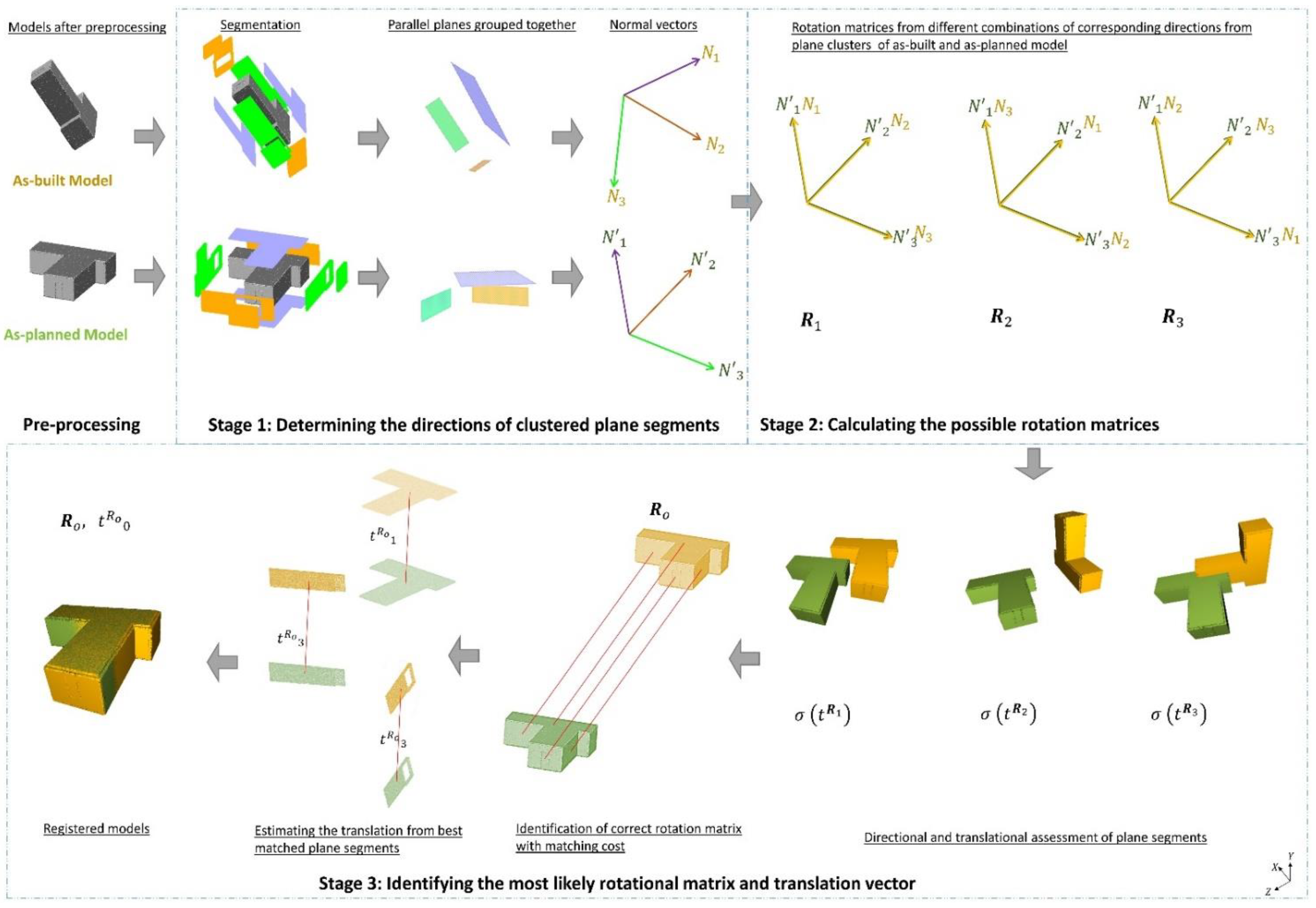
Figure 1. Overall methodology.
Remotesensing 14 01979 g001
Figure 2. Workflow for determining the directions of clustered plane segments.
Remotesensing 14 01979 g002
Figure 3. Visual representation of (a) model, (b) segmented planar components, and (c) planar segments grouped into clusters.
Remotesensing 14 01979 g003
Figure 4. Visualization of (a) plane segment from BIM, (b) plane segment from original point cloud, (c) bounding box of plane segment created from the point cloud, and (d) centroid points calculated from the original point cloud (red) and from the bounding box (blue).
Remotesensing 14 01979 g004
Figure 5. Visualization of (a) possible combinations with directions from the clustered plane segments having the same relative angles in the as-built and as-planned model, (b) normal vectors from as-built (yellow) and as-planned (green) models before rotation (c), the alignment of a pair of corresponding normal vectors after the first rotation, and (d) the aligned normal vectors of both models after the final rotation.
Remotesensing 14 01979 g005
Figure 6. Example of a few rotation matrices and their respective rotational effect on the as-built model against the alignment of the as-planned model, obtained from different possible combinations by aligning the corresponding normal vectors of clustered segments from the as-built (yellow) and as-planned (green) models.
Remotesensing 14 01979 g006
Figure 7. Visualization of the as-built model (yellow) corresponding to the as-planned model (green), with an incorrect orientation (a,b) and correct orientation (c). The lines connecting the matching segments in all orientations represent the corresponding translation.
Remotesensing 14 01979 g007
Figure 8. General workflow for the assessment of the plane segments for each rotation matrix.
Remotesensing 14 01979 g008
Figure 9. Representation of all the possible translation vectors t i , j , are shown with line colors indicating the parallel plane segments from the (a) potential matching planes and (b) matching planes.
Remotesensing 14 01979 g009
Figure 10. Visualization of the corresponding as-built model (yellow) relative to the as-planned model (green) sorted with rotation matrices having matching costs ( σ ) : (a) σ ( t R 1 o ) = 0.4304, (b) σ ( t R 2 o ) = 4.8754, (c)   σ ( t R 3 o ) = 5.0401 and, (d) σ ( t R 4 o ) = 5.5786.
Remotesensing 14 01979 g010
Figure 11. Visualization of the corresponding models registered with different translation vectors computed from the pairs of the most likely matched plane segments sorted according to their matching costs ( σ ) : (a) σ ( t R 0 1 ) = 0.4304, ( b )   σ ( t R 0 2 ) = 0.4361, ( c )   σ ( t R 0 3 ) = 0.4423, ( d )   σ ( t R 0 4 ) = 0.4448, ( e )   σ ( t R 0 5 ) = 0.4783 and, ( f )   σ ( t R 0 6 ) = 0.5874.
Remotesensing 14 01979 g011
Figure 12. Visualization of BIM (as-planned model) and scan (as-built model) from dataset R1, R2, and R3.
Remotesensing 14 01979 g012
Figure 13. Visualization of the registered as-built (yellow) and as-planned (green) models of (a) dataset S1, (b) dataset S2, (c) dataset S3, (d) dataset R1, (e) dataset R2 and, (f) dataset R3.
Remotesensing 14 01979 g013
Figure 14. Graph indicating the processing time and RMSE at different voxel sizes ranging from 0.01 to 0.5 m for dataset 1.
Remotesensing 14 01979 g014
Figure 15. Comparison of computation time of the proposed technique when the as-planned model is processed in a mesh form (left) vs. a point cloud form (right).
Remotesensing 14 01979 g015
Figure 16. Visualization of (a) complete as-planned model, (b) incomplete as-built model with only three plane segments in distinct directions, (c) registered model using translation computed from the centroid of matched segments, and (d) registered model using translation computed from the centroid difference of the complete point cloud.
Remotesensing 14 01979 g016
Table 1. Details of stimulated datasets.
Dataset S1Dataset S2Dataset S3Dataset R1Dataset R2Dataset R3
3D view of
as-built model
Remotesensing 14 01979 i001 Remotesensing 14 01979 i002 Remotesensing 14 01979 i003 Remotesensing 14 01979 i004 Remotesensing 14 01979 i005 Remotesensing 14 01979 i006
Dimensions from top view (m) Remotesensing 14 01979 i007 Remotesensing 14 01979 i008 Remotesensing 14 01979 i009 Remotesensing 14 01979 i010 Remotesensing 14 01979 i011 Remotesensing 14 01979 i012
Height (m)32792.555.2114.6
Area per floor (m2)69Each floor: 39.21st and 2nd floor: 56
3rd floor: 38.8
18.784.21st, 2nd, and 3rd floor:
200
4th floor:
75
No. of plane segments91496610
No. of 3D points in the as-built model1,000,0062,485,9131,364,74179,537,6673,580,30364,773,370
Table 2. Registration details of all the datasets, including the computation of the correct rotation matrix and identical translation.
Dataset No.Dataset S1Dataset S2Dataset S3Dataset R1Dataset R2Dataset R3
No. of plane segments 91496610
No. of directions from plane segment clusters335344
Processing time (s)3.1847.4315.483.965.0123.92
RMSE (mm)7.1869.2788.79218.11923.20517.781
Matching cost
( σ )
According to each possible rotation ( R 1 ,   R 2 ,   R 3 ,   R r ) σ ( t R 1 o ) 0.4301.7870.8252.2141.8663.471
σ ( t R 2 o ) 4.87515.9843.5884.7424.0538.281
σ ( t R 3 o ) 5.04020.7214.3504.9855.09516.335
σ ( t R 4 o ) 5.57821.5714.5225.3837.04719.784
According to the translation of matching plane segments σ ( t R 0 1 ) 0.4301.7870.8252.2141.8663.471
σ ( t R 0 2 ) 0.4361.7950.8252.2351.8763.503
σ ( t R 0 3 ) 0.4421.7970.8302.2902.0903.571
σ ( t R 0 4 ) 0.4441.8000.8552.4772.3643.864
Table 3. Details concerning the processing time and accuracy error according to each dataset.
Dataset No.Processing TimeError
Step 1
(s)
Step 2
(s)
Step 3
(s)
Total Time
(s)
RMSE
(mm)
  ϵ R
(°)
  ϵ t
(mm)
Dataset S10.520.082.583.187.1860.00729.164
Dataset S27.190.0740.1747.439.2780.00740.961
Dataset S32.990.0912.4015.488.7920.00535.385
Dataset R13.230.070.393.6918.1190.02794.267
Dataset R21.820.083.115.0123.2050.020190.482
Dataset R38.10.0815.7423.9217.7810.021107.142
Table 4. Segmented as-built point cloud with different noise levels and voxel sizes.
Voxel Sizes (m)
0.01 m0.13 m0.25 m0.37 m
Standard Deviation of Noise0 Remotesensing 14 01979 i013 Remotesensing 14 01979 i014 Remotesensing 14 01979 i015 Remotesensing 14 01979 i016
0.05 Remotesensing 14 01979 i017 Remotesensing 14 01979 i018 Remotesensing 14 01979 i019 Remotesensing 14 01979 i020
0.1 Remotesensing 14 01979 i021 Remotesensing 14 01979 i022 Remotesensing 14 01979 i023 Remotesensing 14 01979 i024
0.15 Remotesensing 14 01979 i025 Remotesensing 14 01979 i026 Remotesensing 14 01979 i027 Remotesensing 14 01979 i028
Publisher’s Note: MDPI stays neutral with regard to jurisdictional claims in published maps and institutional affiliations.