
Simulating Future LUCC by Coupling Climate Change and Human Effects Based on Multi-Phase Remote Sensing Data

 ,
,
Abstract
:1. Introduction
2. Materials and Methods
2.1. Study Area
2.2. Data Sets and Processing

| Data Set | Category | Data | Year | Resolution | Diagram | Data Resource |
|---|---|---|---|---|---|---|
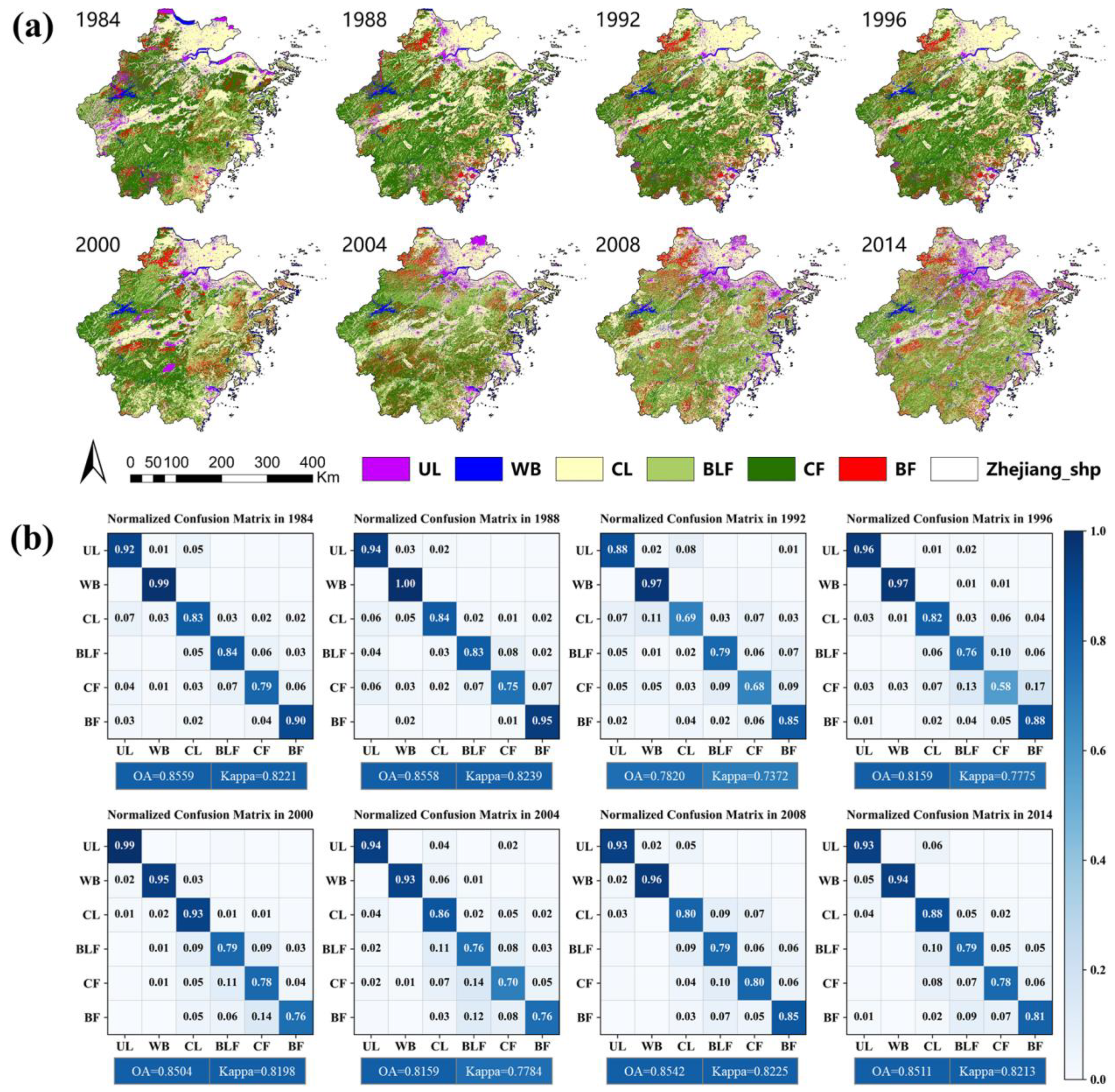
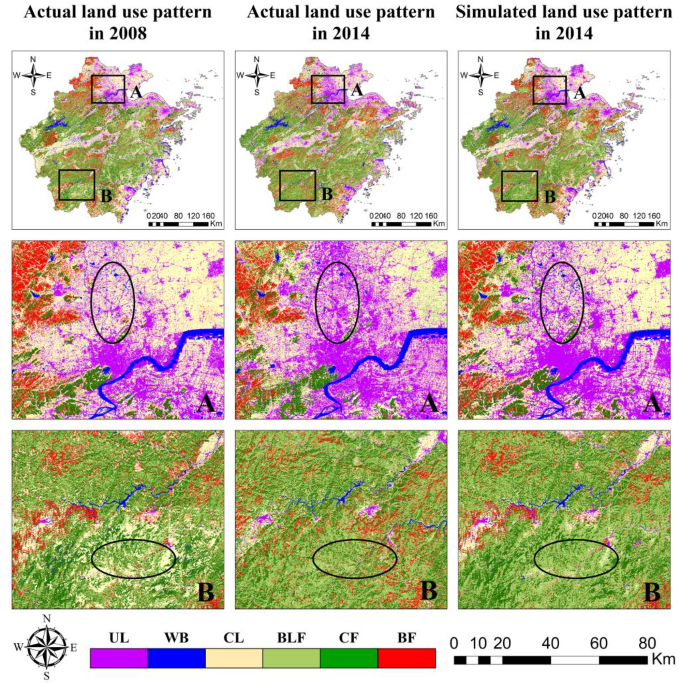
| Geo-spatial data | Land use | Land-use patterns | 1984–2014 | 30 m | Figure 2a,b | The data were based on the Satellite 30 m multispectral data of Landsat-5 TM (1984–2008) and Landsat-8 OLI (2014). After radiation correction, atmospheric correction, and geometric correction, the maximum likelihood classification method was used to obtain land-use patterns. |
| Terrain | DEM | 2014 | 30 m | Figure 3a–c | Downloaded from the Geospatial Data Cloud site (http://www.gscloud.cn, accessed on 24 December 2021). | |
| Slope | Calculated from DEM. | |||||
| Aspect | ||||||
| Soil | Silt fraction | 2008 | 1 km | Figure 3d–i | Silt fraction, clay fraction, sand fraction, and available water content were derived from the Harmonized World Soil Database (HWSD 1.2). The bulk density and soil wilt point were calculated by the silt and clay fraction [41]. | |
| Clay fraction | ||||||
| Sand fraction | ||||||
| Available water content | ||||||
| Bulk density | ||||||
| Wilt point | ||||||
| Climate | Total precipitation | 1984–2014 | 1 km | Figure 3j–m | The annual data were calculated from the averages or sums of the daily data. The daily data were interpolated from observations at 410 meteorological stations in Zhejiang Province and its surrounding provinces using the inverse distance weighted method [42]. | |
| Average temperature | ||||||
| Average radiation | ||||||
| Average relative humidity | ||||||
| Human influence | Population | 2015 | 1 km | Figure 3n,o | Obtained from the Resource and Environmental Science and Data Center of the Chinese Academy of Sciences (http://www.resdc.cn, accessed on 24 December 2021). | |
| Gross domestic product (GDP) | ||||||
| Distance to roads | 2014 | 30 m | Figure 3p–r | Calculated from the vector maps of the roads, the railways, and the water systems, which were downloaded from the Open Street map (https://www.openstreetmap.org/, accessed on 12 October 2020). | ||
| Distance to railways | ||||||
| Distance to water | ||||||
| Macro statistics data | Land-use area | 1984–2014 | - | - | Calculated from the land-use patterns. | |
| Total precipitation statistics | - | Calculated from the total precipitation. | ||||
| Average temperature statistics | - | Calculated from the average temperature. | ||||
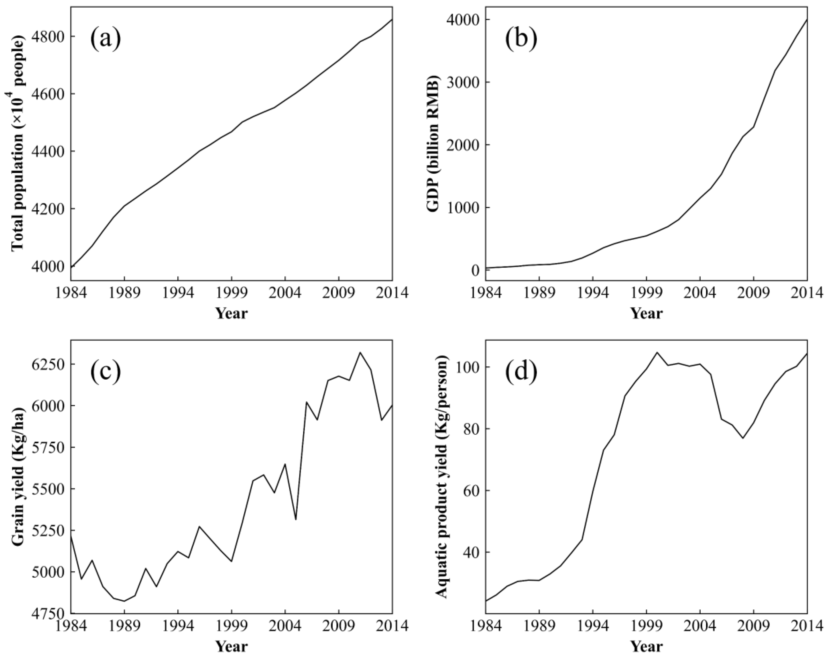
| Population statistics | Figure 4a–d | Collected from the Zhejiang Statistical Yearbook (http://tjj.zj.gov.cn/, accessed on 12 October 2020). | ||||
| GDP statistics | ||||||
| Grain yield | ||||||
| Aquatic product yield | ||||||
| Forest coverage rate | 2004–2020 | Figure 1c | Collected from the Announcement of Forest Resources and Its Ecological Function Value of Zhejiang Province (http://lyj.zj.gov.cn/index.html, accessed on 24 December 2021). | |||
| Sample plots data | Classification verification plots | 1984–2014 | - | Figure 1b and Table 2 | Classification verification plots of BLF, CF, and BF were derived from the data of the National Forest Inventory. Verification plots of other land-use types were based on field investigation and image visual interpretation. | |
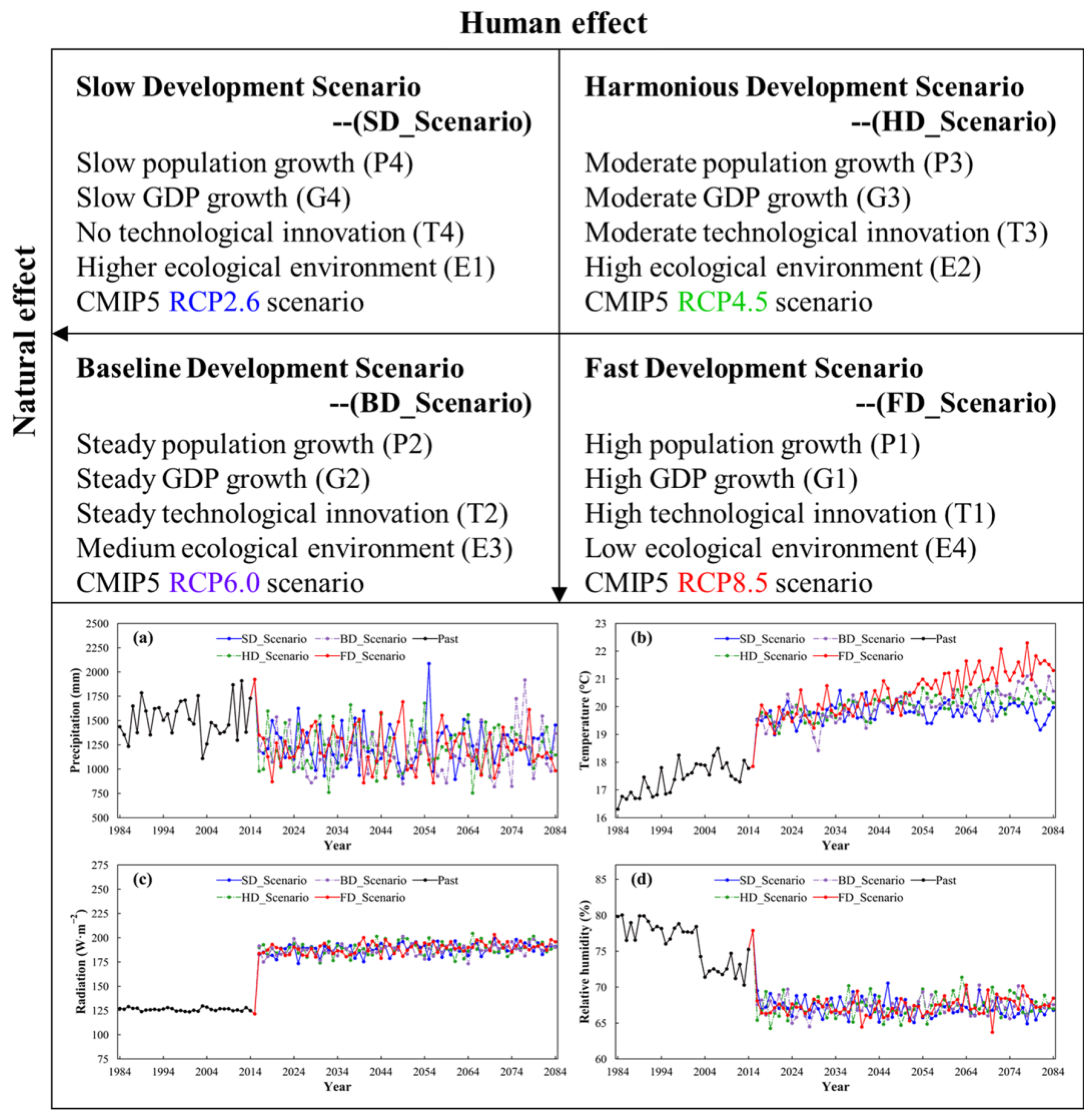
2.3. Future Scenario Description
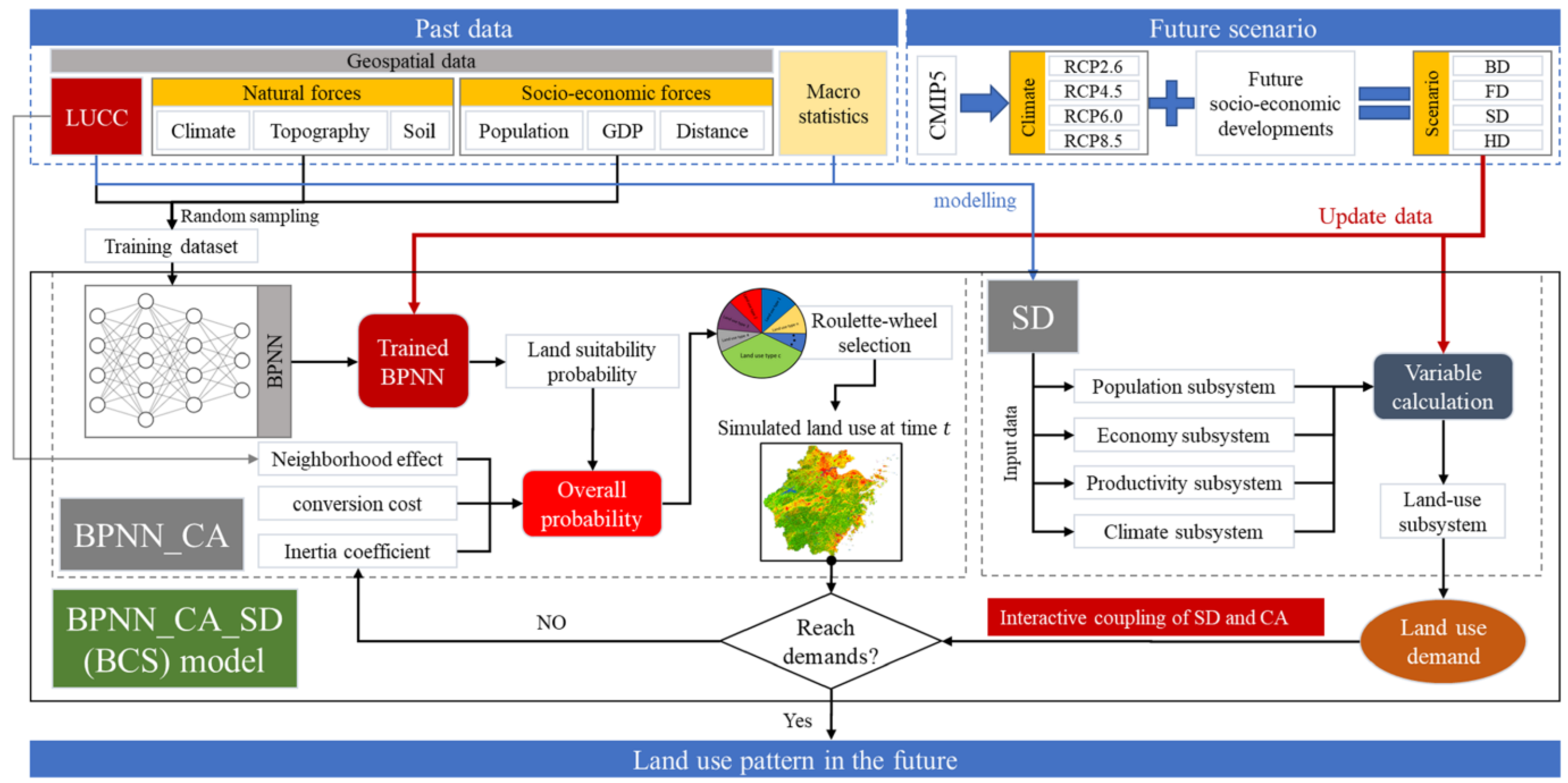
2.4. Methodology
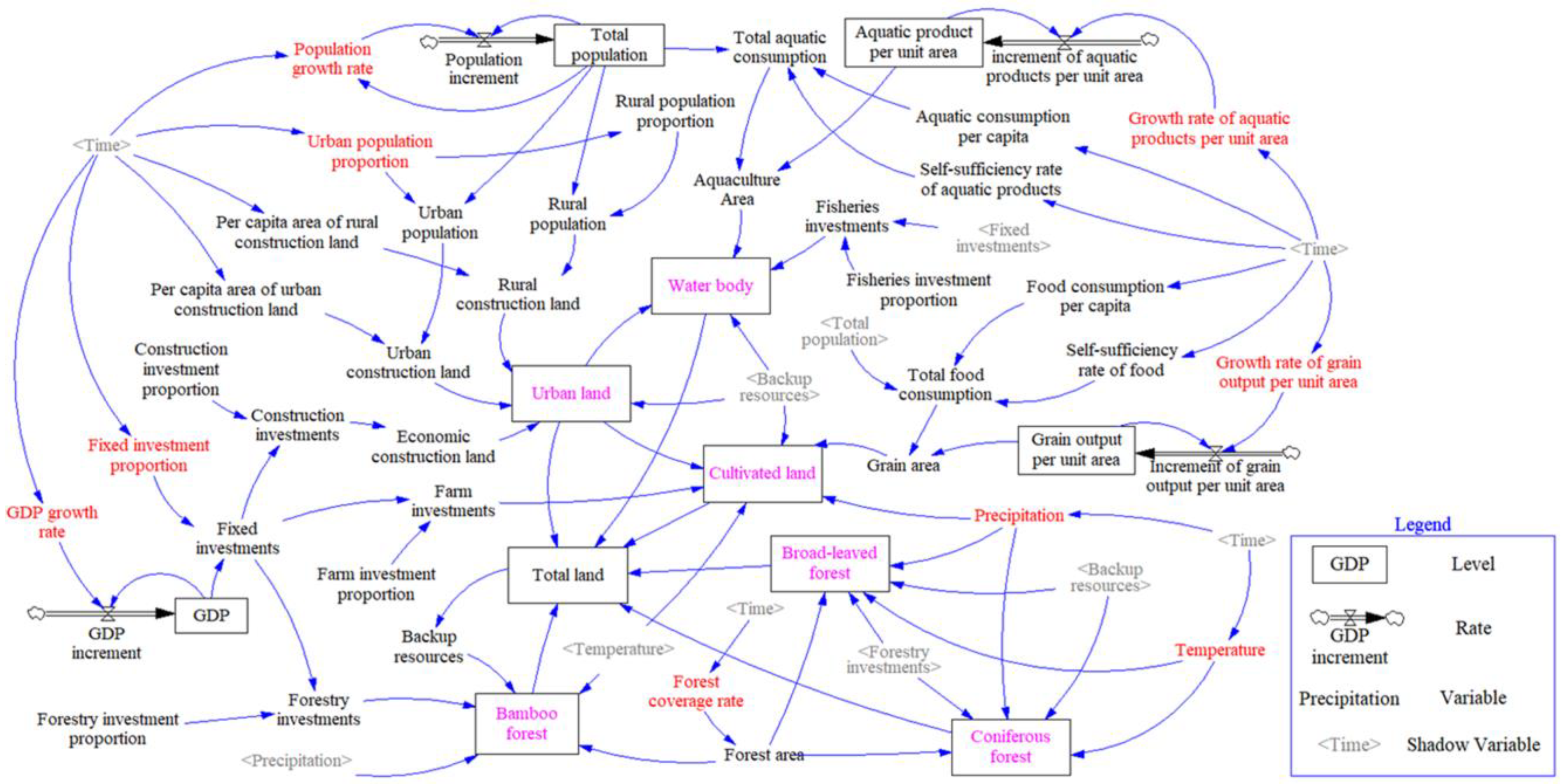
2.4.1. SD Model
2.4.2. BPNN_CA Model
| Algorithm 1: Train BPNN with the minibatch Adam optimization algorithm. |
| initialize () |
| for = 1, …, do |
| for = 1, …, # do |
| uniformly sample images |
| , preprocess(images) |
| forward (net, ) |
| loss (, ) |
| , backpropagation () |
| update (, , ) |
| end for |
| end for |
| Algorithm 2: Using a roulette-wheel selection mechanism to allocate the probability. |
| input: |
| a uniformly distributed random number ranging from 0 to 1 |
| for= 1, …, do |
| if then |
| break |
| else |
| continue |
| end for |
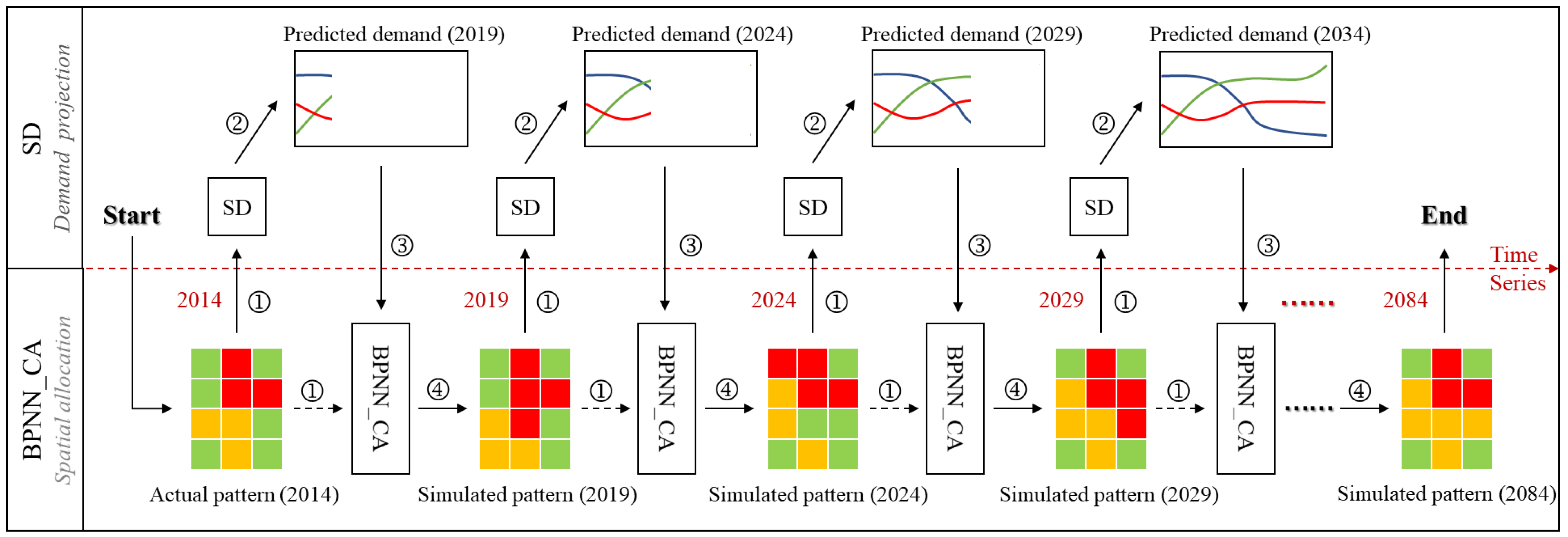
2.4.3. Interactive Integration of the BCS Model
2.4.4. Assessment Methods of the BCS Model
3. Results
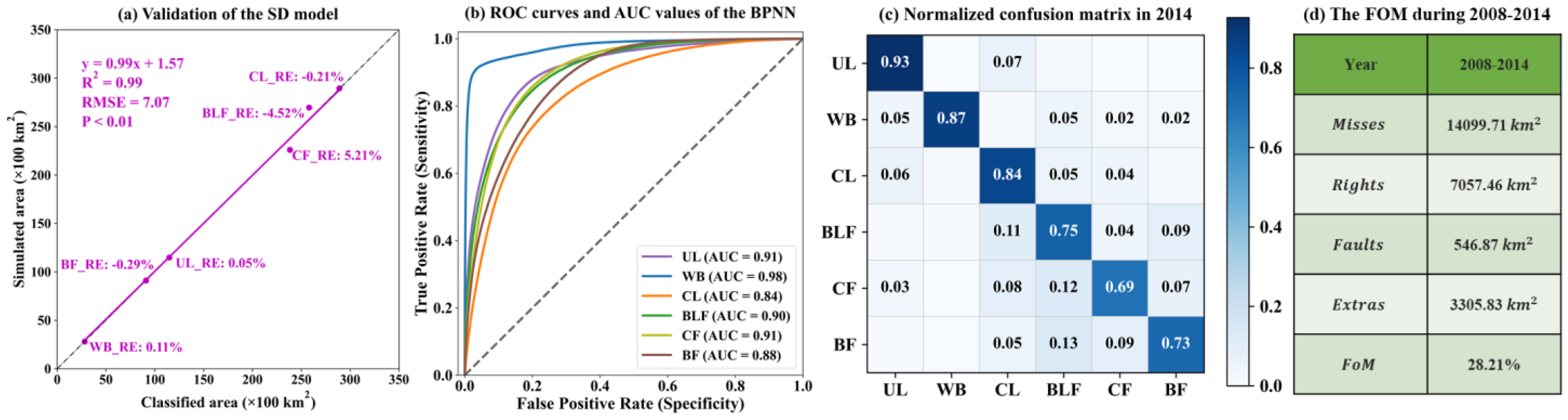
3.1. Model Validations
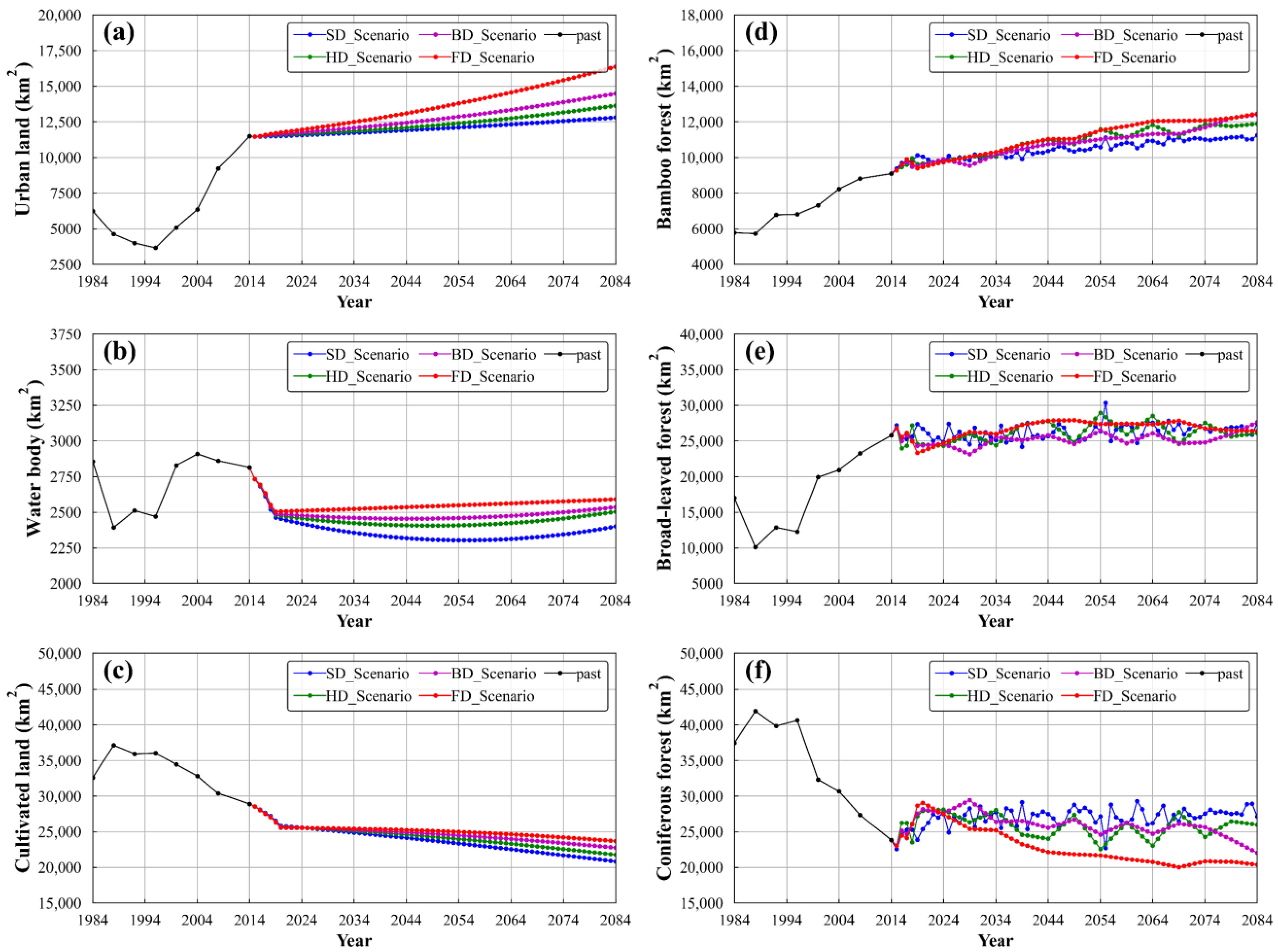
3.2. Future Land Use Demand Projection
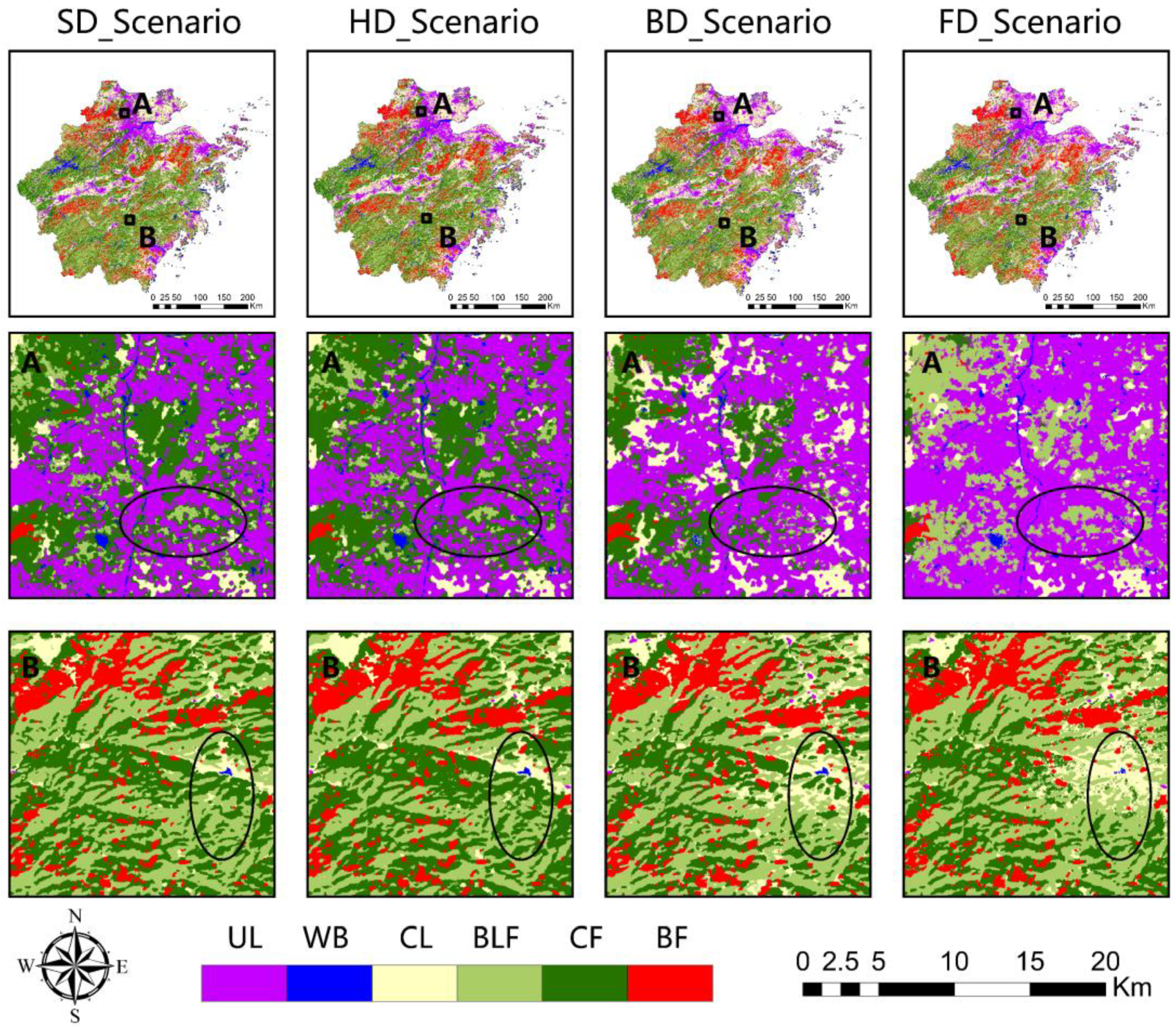
3.3. Future Spatiotemporal Land-Use Pattern
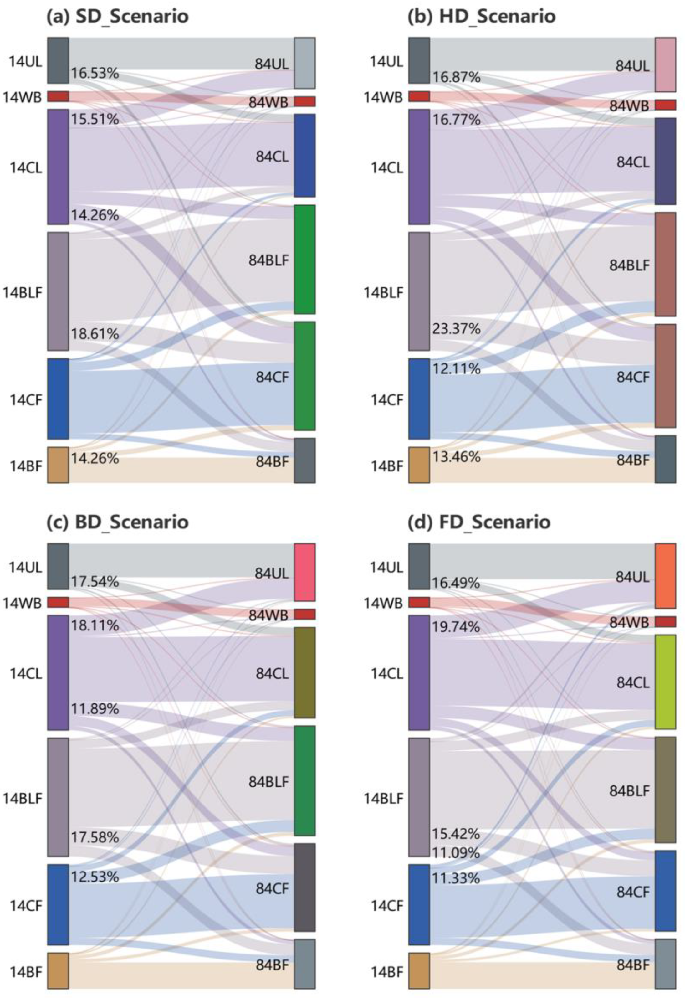
3.4. Analysis of Future Land-Use Conversion
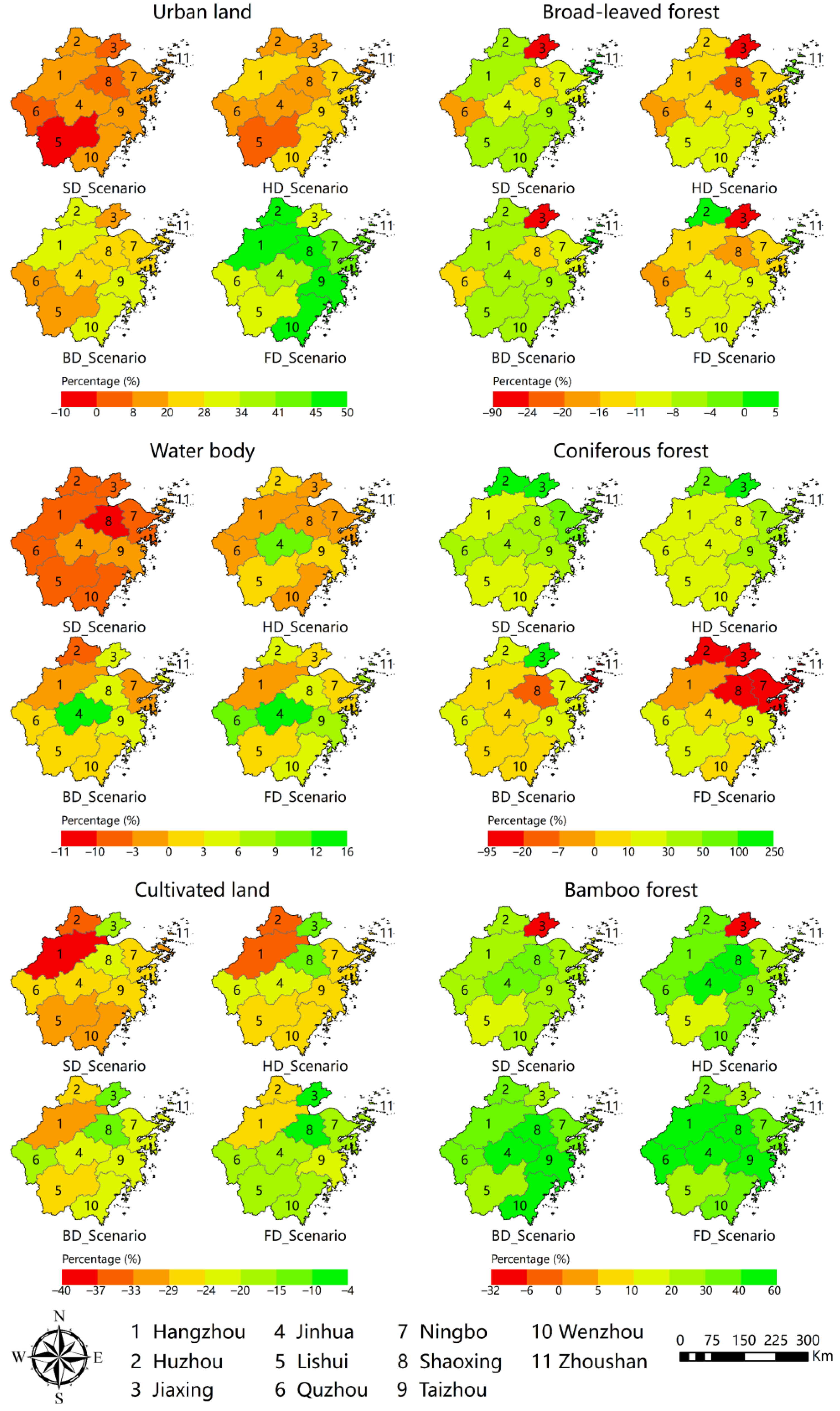
3.5. Analysis of Land-Use Change Amplitude at the Administrative Level
4. Discussion
4.1. Future Enhancements of the BCS Model
4.2. Future Strategy for Land-Use Management
5. Conclusions
Author Contributions
Funding
Institutional Review Board Statement
Informed Consent Statement
Data Availability Statement
Acknowledgments
Conflicts of Interest
Abbreviations
| Abbreviation | Description |
| LUCC | Land Use and Land Cover Change |
| UL | Urban Land |
| WB | Water Body |
| CL | Cultivated Land |
| BLF | Broad-Leaved Forest |
| CF | Coniferous Forest |
| BF | Bamboo Forest |
| CA | Cellular Automata |
| SD | System Dynamics |
| BPNN | Back Propagation Neural Network |
| BPNN_CA | CA Model Integrated with the BPNN |
| BCS | BPNN_CA Model Integrated with the SD |
| CLUE-S | The Conversion of Land Use and Its Effects at the Small Regional Extent |
| OA | Overall Accuracy |
| Kappa | Kappa Coefficients |
| PA | Producer’s Accuracy |
| ROC | Receiver Operating Characteristic |
| AUC | Area under ROC Curve |
| Figure of Merit | |
| SD_Scenario | Slow Development Scenario |
| HD_Scenario | Harmonious Development Scenario |
| BD_Scenario | Base Development Scenario |
| FD_Scenario | Fast Development Scenario |
| RCP | Representative Concentration Pathway |
| CMIP5 | Coupled Model Intercomparison Project 5 |
| IPCC | Intergovernmental Panel on Climate Change |
References
- Jiao, J.-G.; Yang, L.-Z.; Wu, J.-X.; Wang, H.-Q.; Li, H.-X.; Ellis, E.C. Land use and soil organic carbon in China’s village landscapes. Pedosphere 2010, 20, 1–14. [Google Scholar] [CrossRef] [Green Version]
- Matthews, H.D.; Graham, T.L.; Keverian, S.; Lamontagne, C.; Seto, D.; Smith, T.J. National contributions to observed global warming. Environ. Res. Lett. 2014, 9, 468–475. [Google Scholar] [CrossRef] [Green Version]
- Su, Z.-Y.; Xiong, Y.-M.; Zhu, J.-Y.; Ye, Y.-C.; Ye, M. Soil organic carbon content and distribution in a small landscape of Dongguan, South China. Pedosphere 2006, 16, 10–17. [Google Scholar] [CrossRef]
- Yue, C.; Ciais, P.; Houghton, R.A.; Nassikas, A.A. Contribution of land use to the interannual variability of the land carbon cycle. Nat. Commun. 2020, 11, 1–11. [Google Scholar] [CrossRef] [PubMed]
- Yu, Z.; Lu, C.; Tian, H.; Canadell, J.G. Largely underestimated carbon emission from land use and land cover change in the conterminous United States. Glob. Chang. Biol. 2019, 25, 3741–3752. [Google Scholar] [CrossRef] [PubMed]
- Brovkin, V.; Boysen, L.; Arora, V.K.; Boisier, J.P.; Cadule, P.; Chini, L.; Claussen, M.; Friedlingstein, P.; Gayler, V.; van den Hurk, B.J.J.M.; et al. Effect of anthropogenic land-use and land-cover changes on climate and land carbon storage in CMIP5 projections for the twenty-first century. J. Clim. 2013, 26, 6859–6881. [Google Scholar] [CrossRef]
- Khoshnood Motlagh, S.; Sadoddin, A.; Haghnegahdar, A.; Razavi, S.; Salmanmahiny, A.; Ghorbani, K. Analysis and prediction of land cover changes using the land change modeler (LCM) in a semiarid river basin, Iran. Land. Degrad. Dev. 2021, 32, 3092–3105. [Google Scholar] [CrossRef]
- Rasmussen, L.V.; Rasmussen, K.; Reenberg, A.; Proud, S. A system dynamics approach to land use changes in agro-pastoral systems on the desert margins of Sahel. Agric. Syst. 2012, 107, 56–64. [Google Scholar] [CrossRef]
- Liu, D.; Zheng, X.; Zhang, C.; Wang, H. A new temporal–spatial dynamics method of simulating land-use change. Ecol. Model. 2017, 350, 1–10. [Google Scholar] [CrossRef]
- Liu, X.; Ou, J.; Li, X.; Ai, B. Combining system dynamics and hybrid particle swarm optimization for land use allocation. Ecol. Model. 2013, 257, 11–24. [Google Scholar] [CrossRef]
- Zheng, X.-Q.; Zhao, L.; Xiang, W.-N.; Li, N.; Lv, L.-N.; Yang, X. A coupled model for simulating spatio-temporal dynamics of land-use change: A case study in Changqing, Jinan, China. Landsc. Urban Plan. 2012, 106, 51–61. [Google Scholar] [CrossRef]
- Luo, G.; Yin, C.; Chen, X.; Xu, W.; Lu, L. Combining system dynamic model and CLUE-S model to improve land use scenario analyses at regional scale: A case study of Sangong watershed in Xinjiang, China. Ecol. Complex. 2010, 7, 198–207. [Google Scholar] [CrossRef]
- Jiao, M.; Hu, M.; Xia, B. Spatiotemporal dynamic simulation of land-use and landscape-pattern in the Pearl River Delta, China. Sustain. Cities Soc. 2019, 49, 101581. [Google Scholar] [CrossRef]
- Zhang, Y.; Li, Y.; Lv, J.; Wang, J.; Wu, Y. Scenario simulation of ecological risk based on land use/cover change—A case study of the Jinghe county, China. Ecol. Indic. 2021, 131, 108176. [Google Scholar] [CrossRef]
- Gomes, E.; Inácio, M.; Bogdzevič, K.; Kalinauskas, M.; Karnauskaitė, D.; Pereira, P. Future land-use changes and its impacts on terrestrial ecosystem services: A review. Sci. Total Environ. 2021, 781, 146716. [Google Scholar] [CrossRef]
- He, M.; Chen, C.; Zheng, F.; Chen, Q.; Zhang, J.; Yan, H.; Lin, Y. An efficient dynamic route optimization for urban flooding evacuation based on Cellular Automata. Comput. Environ. Urban Syst. 2021, 87, 101622. [Google Scholar] [CrossRef]
- Priem, F.; Canters, F. Modelling transitions in sealed surface cover fraction with Quantitative State Cellular Automata. Landsc. Urban Plan. 2021, 211, 104081. [Google Scholar] [CrossRef]
- Aguejdad, R. The Influence of the Calibration Interval on Simulating Non-Stationary Urban Growth Dynamic Using CA-Markov Model. Remote Sens. 2021, 13, 468. [Google Scholar] [CrossRef]
- Li, K.; Feng, M.; Biswas, A.; Su, H.; Niu, Y.; Cao, J. Driving Factors and Future Prediction of Land Use and Cover Change Based on Satellite Remote Sensing Data by the LCM Model: A Case Study from Gansu Province, China. Sensors 2020, 20, 2757. [Google Scholar] [CrossRef]
- Surabuddin Mondal, M.; Sharma, N.; Kappas, M.; Garg, P.K. Modeling of spatio-temporal dynamics of land use and land cover in a part of Brahmaputra River basin using Geoinformatic techniques. Geocarto. Int. 2013, 28, 632–656. [Google Scholar] [CrossRef]
- Jokar Arsanjani, J.; Helbich, M.; Kainz, W.; Darvishi Boloorani, A. Integration of logistic regression, Markov chain and cellular automata models to simulate urban expansion. Int. J. Appl. Earth Obs. Geoinf. 2013, 21, 265–275. [Google Scholar] [CrossRef]
- Mallick, J.; AlQadhi, S.; Talukdar, S.; Pradhan, B.; Bindajam, A.A.; Islam, A.R.M.T.; Dajam, A.S. A Novel Technique for Modeling Ecosystem Health Condition: A Case Study in Saudi Arabia. Remote Sens. 2021, 13, 2632. [Google Scholar] [CrossRef]
- Roodposhti, M.S.; Aryal, J.; Bryan, B.A. A novel algorithm for calculating transition potential in cellular automata models of land-use/cover change. Environ. Model. Software 2019, 112, 70–81. [Google Scholar] [CrossRef]
- Chen, Z.; Huang, M.; Zhu, D.; Altan, O. Integrating Remote Sensing and a Markov-FLUS Model to Simulate Future Land Use Changes in Hokkaido, Japan. Remote Sens. 2021, 13, 2621. [Google Scholar] [CrossRef]
- Marondedze, A.K.; Schütt, B. Predicting the Impact of Future Land Use and Climate Change on Potential Soil Erosion Risk in an Urban District of the Harare Metropolitan Province, Zimbabwe. Remote Sens. 2021, 13, 4360. [Google Scholar] [CrossRef]
- Liu, X.; Liang, X.; Li, X.; Xu, X.; Ou, J.; Chen, Y.; Li, S.; Wang, S.; Pei, F. A future land use simulation model (FLUS) for simulating multiple land use scenarios by coupling human and natural effects. Landsc. Urban Plan. 2017, 168, 94–116. [Google Scholar] [CrossRef]
- Liu, Y.; Jing, W.; Xu, L. Parallelizing backpropagation neural network using MapReduce and cascading model. Comput. Intell. Neurosci. 2016, 2016, 1–11. [Google Scholar] [CrossRef] [Green Version]
- Zhou, G.; Liu, S.; Li, Z.; Zhang, D.; Tang, X.; Zhou, C.; Yan, J.; Mo, J. Old-growth forests can accumulate carbon in soils. Science 2006, 314, 1417. [Google Scholar] [CrossRef] [Green Version]
- Tan, Z.-H.; Zhang, Y.-P.; Schaefer, D.; Yu, G.-R.; Liang, N.; Song, Q.-H. An old-growth subtropical Asian evergreen forest as a large carbon sink. Atmos. Environ. 2011, 45, 1548–1554. [Google Scholar] [CrossRef]
- Fang, J.; Yu, G.; Liu, L.; Hu, S.; Chapin, F.S. Climate change, human impacts, and carbon sequestration in China. Proc. Natl. Acad. Sci. USA 2018, 115, 4015–4020. [Google Scholar] [CrossRef] [Green Version]
- Liu, F.-h.; Xu, C.-Y.; Yang, X.-x.; Ye, X.-c. Controls of climate and land-use change on terrestrial net primary productivity variation in a subtropical humid basin. Remote Sens. 2020, 12, 3525. [Google Scholar] [CrossRef]
- Guo, X.; Chen, H.Y.H.; Meng, M.; Biswas, S.R.; Ye, L.; Zhang, J. Effects of land use change on the composition of soil microbial communities in a managed subtropical forest. For. Ecol. Manag. 2016, 373, 93–99. [Google Scholar] [CrossRef]
- Zhu, K.; Zhang, J.; Niu, S.; Chu, C.; Luo, Y. Limits to growth of forest biomass carbon sink under climate change. Nat. Commun. 2018, 9, 2709. [Google Scholar] [CrossRef] [PubMed] [Green Version]
- Yao, Y.; Piao, S.; Wang, T. Future biomass carbon sequestration capacity of Chinese forests. Sci. Bull. 2018, 63, 1108–1117. [Google Scholar] [CrossRef] [Green Version]
- Poelmans, L.; Van Rompaey, A. Complexity and performance of urban expansion models. Comput. Environ. Urban Syst. 2010, 34, 17–27. [Google Scholar] [CrossRef]
- Feng, Y.; Tong, X. Incorporation of spatial heterogeneity-weighted neighborhood into cellular automata for dynamic urban growth simulation. GISci. Remote Sens. 2019, 56, 1024–1045. [Google Scholar] [CrossRef]
- Van Vuuren, D.P.; Edmonds, J.; Kainuma, M.; Riahi, K.; Thomson, A.; Hibbard, K.; Hurtt, G.C.; Kram, T.; Krey, V.; Lamarque, J.-F.; et al. The representative concentration pathways: An overview. Clim. Chang. 2011, 109, 5–31. [Google Scholar] [CrossRef]
- Jefferson, M. IPCC fifth assessment synthesis report: “Climate change 2014: Longer report”: Critical analysis. Technol. Forecast. Soc. Chang. 2015, 92, 362–363. [Google Scholar] [CrossRef]
- Li, J.; Chen, X.; Kurban, A.; Van de Voorde, T.; De Maeyer, P.; Zhang, C. Coupled SSPs-RCPs scenarios to project the future dynamic variations of water-soil-carbon-biodiversity services in Central Asia. Ecol. Indic. 2021, 129, 107936. [Google Scholar] [CrossRef]
- Dubovyk, O.; Sliuzas, R.; Flacke, J. Spatio-temporal modelling of informal settlement development in Sancaktepe district, Istanbul, Turkey. ISPRS J. Photogramm. Remote Sens. 2011, 66, 235–246. [Google Scholar] [CrossRef]
- Zheng, J.; Mao, F.; Du, H.; Li, X.; Zhou, G.; Dong, L.; Zhang, M.; Han, N.; Liu, T.; Xing, L. Spatiotemporal simulation of net ecosystem productivity and its response to climate change in subtropical forests. Forests 2019, 10, 708. [Google Scholar] [CrossRef] [Green Version]
- Li, X.; Du, H.; Mao, F.; Zhou, G.; Xing, L.; Liu, T.; Han, N.; Liu, E.; Ge, H.; Liu, Y.; et al. Mapping spatiotemporal decisions for sustainable productivity of bamboo forest land. Land. Degrad. Dev. 2020, 31, 939–958. [Google Scholar] [CrossRef]
- Li, Y.; Han, N.; Li, X.; Du, H.; Mao, F.; Cui, L.; Liu, T.; Xing, L. Spatiotemporal estimation of bamboo forest aboveground carbon storage based on Landsat data in Zhejiang, China. Remote Sensing 2018, 10, 898. [Google Scholar] [CrossRef] [Green Version]
- Zhang, M.; Du, H.; Mao, F.; Zhou, G.; Li, X.; Dong, L.; Zheng, J.; Zhu, D.e.; Liu, H.; Huang, Z.; et al. Spatiotemporal evolution of urban expansion using Landsat time series data and assessment of its influences on forests. ISPRS Int. J. Geoinf. 2020, 9, 64. [Google Scholar] [CrossRef] [Green Version]
- Li, X.; Mao, F.; Du, H.; Zhou, G.; Xing, L.; Liu, T.; Han, N.; Liu, Y.; Zhu, D.e.; Zheng, J.; et al. Spatiotemporal evolution and impacts of climate change on bamboo distribution in China. J. Environ. Manag. 2019, 248, 109265. [Google Scholar] [CrossRef]
- Tian, H.; Liang, X.; Li, X.; Liu, X.; Ou, J.; Hong, Y.; He, Z. Simulating Multiple Land Use Scenarios in China during 2010–2050 Based on System Dynamic Model. Trop. Geogr. 2017, 37, 547–561. [Google Scholar]
- Vuuren, D.; Stehfest, E.; Elzen, M.; Kram, T.; Vliet, J.V.; Deetman, S.; Isaac, M.; Goldewijk, K.K.; Hof, A.; Beltran, A.M. RCP2.6: Exploring the possibility to keep global mean temperature increase below 2°C. Clim. Chang. 2011, 109, 95–116. [Google Scholar] [CrossRef]
- Chaturvedi, R.K.; Joshi, J.; Jayaraman, M.; Bala, G.; Ravindranath, N. Multi-model climate change projections for India under representative concentration pathways. Curr. Sci. 2012, 103, 791–802. [Google Scholar]
- Riahi, K.; Rao, S.; Krey, V.; Cho, C.; Chirkov, V.; Fischer, G.; Kindermann, G.; Nakicenovic, N.; Rafaj, P. RCP 8.5—A scenario of comparatively high greenhouse gas emissions. Clim. Chang. 2011, 109, 33–57. [Google Scholar] [CrossRef] [Green Version]
- Zou, L.; Zhou, T. Near future (2016–40) summer precipitation changes over China as projected by a regional climate model (RCM) under the RCP8.5 emissions scenario: Comparison between RCM downscaling and the driving GCM. Adv. Atmos. Sci. 2013, 30, 806–818. [Google Scholar] [CrossRef]
- Xu, X.; Du, Z.; Zhang, H. Integrating the system dynamic and cellular automata models to predict land use and land cover change. Int. J. Appl. Earth Obs. Geoinf. 2016, 52, 568–579. [Google Scholar] [CrossRef]
- Liang, X.; Guan, Q.; Clarke, K.C.; Liu, S.; Wang, B.; Yao, Y. Understanding the drivers of sustainable land expansion using a patch-generating land use simulation (PLUS) model: A case study in Wuhan, China. Comput. Environ. Urban Syst. 2021, 85, 101569. [Google Scholar] [CrossRef]
- Xu, H.; Song, Y.; Tian, Y. Simulation of land-use pattern evolution in hilly mountainous areas of North China: A case study in Jincheng. Land Use Policy 2022, 112, 105826. [Google Scholar] [CrossRef]
- Pontius, R.G.; Boersma, W.; Castella, J.; Clarke, K.C.; De Nijs, T.; Dietzel, C.; Duan, Z.; Fotsing, E.; Goldstein, N.; Kok, K. Comparing the input, output, and validation maps for several models of land change. Ann. Regional Sci. 2008, 42, 11–37. [Google Scholar] [CrossRef] [Green Version]
- Wu, Z.; Dai, E.; Wu, Z.; Lin, M. Future forest dynamics under climate change, land use change, and harvest in subtropical forests in Southern China. Landsc. Ecol. 2019, 34, 843–863. [Google Scholar] [CrossRef]
- Reimann, L.; Jones, B.; Nikoletopoulos, T.; Vafeidis, A.T. Accounting for internal migration in spatial population projections—A gravity-based modeling approach using the Shared Socioeconomic Pathways. Environ. Res. Lett. 2021, 16, 074025. [Google Scholar] [CrossRef]


| Year | UL | WB | CL | BLF | CF | BF | Total |
|---|---|---|---|---|---|---|---|
| 1984 | 151 | 141 | 302 | 204 | 385 | 114 | 1297 |
| 1988 | 157 | 104 | 287 | 164 | 317 | 149 | 1178 |
| 1992 | 163 | 112 | 237 | 196 | 266 | 182 | 1156 |
| 1996 | 177 | 134 | 267 | 144 | 215 | 170 | 1107 |
| 2000 | 128 | 146 | 139 | 159 | 165 | 232 | 969 |
| 2004 | 128 | 142 | 139 | 142 | 152 | 215 | 918 |
| 2008 | 123 | 128 | 127 | 127 | 127 | 246 | 878 |
| 2014 | 123 | 132 | 138 | 147 | 154 | 139 | 833 |
| Factors | Patterns | Annual Growth Rate Settings from 2014 to 2084 | |
|---|---|---|---|
| Population | High growth (P1) | 7.2‰ average from 2004 to 2014 | |
| Steady growth (P2) | Growth rate simulated by logistic population retardation growth model | ||
| Moderate growth (P3) | 0.85× growth rate simulated by logistic population retardation growth model | ||
| Slow growth (P4) | 7.2‰ linearly down to 3.4‰ | ||
| GDP | High growth (G1) | 14% average from 2004 to 2014 | |
| Steady growth (G2) | 14% linearly down to 10.5% | ||
| Moderate growth (G3) | 14% linearly down to 8% | ||
| Slow growth (G4) | 14% linearly down to 6.5% | ||
| Technology | Rapid innovation (T1) | Grain yield | Maintain 5‰ in 2014 |
| Aquatic yield | Maintain 8% in 2014 | ||
| Steady innovation (T2) | Grain yield | 5‰ linearly down to 3‰ | |
| Aquatic yield | 8% linearly down to 5% | ||
| Moderate innovation (T3) | Grain yield | 5% linearly down to 1% | |
| Aquatic yield | 8% linearly down to 2% | ||
| No innovation (T4) | Grain yield | 0% | |
| Aquatic yield | 0% | ||
| Ecology | Higher forest coverage rate (E1) High forest coverage rate (E2) Medium forest coverage rate (E3) Low forest coverage rate (E4) | 60.89% linearly up to 65% | |
| 60.89% linearly up to 63% | |||
| 60.89% linearly up to 61% | |||
| 60.89% linearly down to 60% | |||
| Types | UL | WB | CL | BLF | CF | BF |
|---|---|---|---|---|---|---|
| UL | 0 | 0.85 | 0.7 | 0.99 | 0.99 | 0.99 |
| WB | 0.8 | 0 | 0.8 | 0.9 | 0.9 | 0.9 |
| CL | 0.3 | 0.7 | 0 | 0.5 | 0.4 | 0.5 |
| BLF | 0.9 | 0.9 | 0.7 | 0 | 0.6 | 0.5 |
| CF | 0.9 | 0.9 | 0.6 | 0.5 | 0 | 0.6 |
| BF | 0.9 | 0.9 | 0.7 | 0.6 | 0.6 | 0 |
Publisher’s Note: MDPI stays neutral with regard to jurisdictional claims in published maps and institutional affiliations. |
© 2022 by the authors. Licensee MDPI, Basel, Switzerland. This article is an open access article distributed under the terms and conditions of the Creative Commons Attribution (CC BY) license (https://creativecommons.org/licenses/by/4.0/).
Share and Cite
Huang, Z.; Li, X.; Du, H.; Mao, F.; Han, N.; Fan, W.; Xu, Y.; Luo, X. Simulating Future LUCC by Coupling Climate Change and Human Effects Based on Multi-Phase Remote Sensing Data. Remote Sens. 2022, 14, 1698. https://doi.org/10.3390/rs14071698
Huang Z, Li X, Du H, Mao F, Han N, Fan W, Xu Y, Luo X. Simulating Future LUCC by Coupling Climate Change and Human Effects Based on Multi-Phase Remote Sensing Data. Remote Sensing. 2022; 14(7):1698. https://doi.org/10.3390/rs14071698
Chicago/Turabian StyleHuang, Zihao, Xuejian Li, Huaqiang Du, Fangjie Mao, Ning Han, Weiliang Fan, Yanxin Xu, and Xin Luo. 2022. "Simulating Future LUCC by Coupling Climate Change and Human Effects Based on Multi-Phase Remote Sensing Data" Remote Sensing 14, no. 7: 1698. https://doi.org/10.3390/rs14071698
APA StyleHuang, Z., Li, X., Du, H., Mao, F., Han, N., Fan, W., Xu, Y., & Luo, X. (2022). Simulating Future LUCC by Coupling Climate Change and Human Effects Based on Multi-Phase Remote Sensing Data. Remote Sensing, 14(7), 1698. https://doi.org/10.3390/rs14071698