
Using Eco-Geographical Zoning Data and Crowdsourcing to Improve the Detection of Spurious Land Cover Changes


Abstract
:1. Introduction
1.1. Land Cover Change Detection Methods
1.2. Main Reasons for Spurious Changes
- (1)
- Bitemporal images are usually acquired under different atmospheric conditions, including different sun heights, sun angles, and off-nadir distances, which result in varying illumination levels in dual images. Sood et al. [13] focused on the problem of change caused by different shadows in high mountain areas and found that, in mountainous regions, satellite imagery change detection is more complex due to the presence of a rugged topography, slope variability, and topographic (shadow) effects. As a result, a topographically controlled subpixel-based change detection model was used to reduce the detection of spurious pixels. To remove the false change in vegetation resulting from building shadows caused by the shooting angle and sunlight in urban high-resolution aerial change detection, Zhou et al. [14] adopted a series of spatial analyses at different levels and reduced spurious changes. Spatial analysis was mainly conducted using self-adaptive morphology;
- (2)
- Large differences in dryness or humidity between the two phases—for example, abundant precipitation in one phase and scarce precipitation in another phase—result in a large difference in soil moisture, and a change in the position of the boundary lines of rivers and lakes. Similar examples occur for other land types, including grassland before and after wilting, and wetlands when water levels change;
- (3)
- Bitemporal images with various types of phenological phenomena may be acquired at different collection times that cover the same area. For example, the ground reflectivity values of farmland in various agricultural pheno-phases are different before and after harvesting. The landscape is different in summer and winter due to the changes that occur across the four seasons. Deciduous forests have varied spectral characteristics in different seasons. Grassland turns yellow and withers in autumn and winter, and turns green in spring. Lu et al. [15] used Landsat images from March and June in different years in the Shanxi Province of China for change detection to test a method intended to weaken spurious change. June was the peak period, whereas no crops were planted in March. The evident differences in the spectrum of cultivated land found by Lu et al. were due to the influence of phenology; hence, change detection has many false changes;
- (4)
- Forestland is affected by pests or diseases. Dendrolimus punctatus, Bursaphelenchus xylophilus, desert locust, pine leaf bee, and gypsy moth all lead to corresponding changes in spectral brightness and greenness [16];
- (5)
1.3. Review of Spurious Change Alleviation Methods
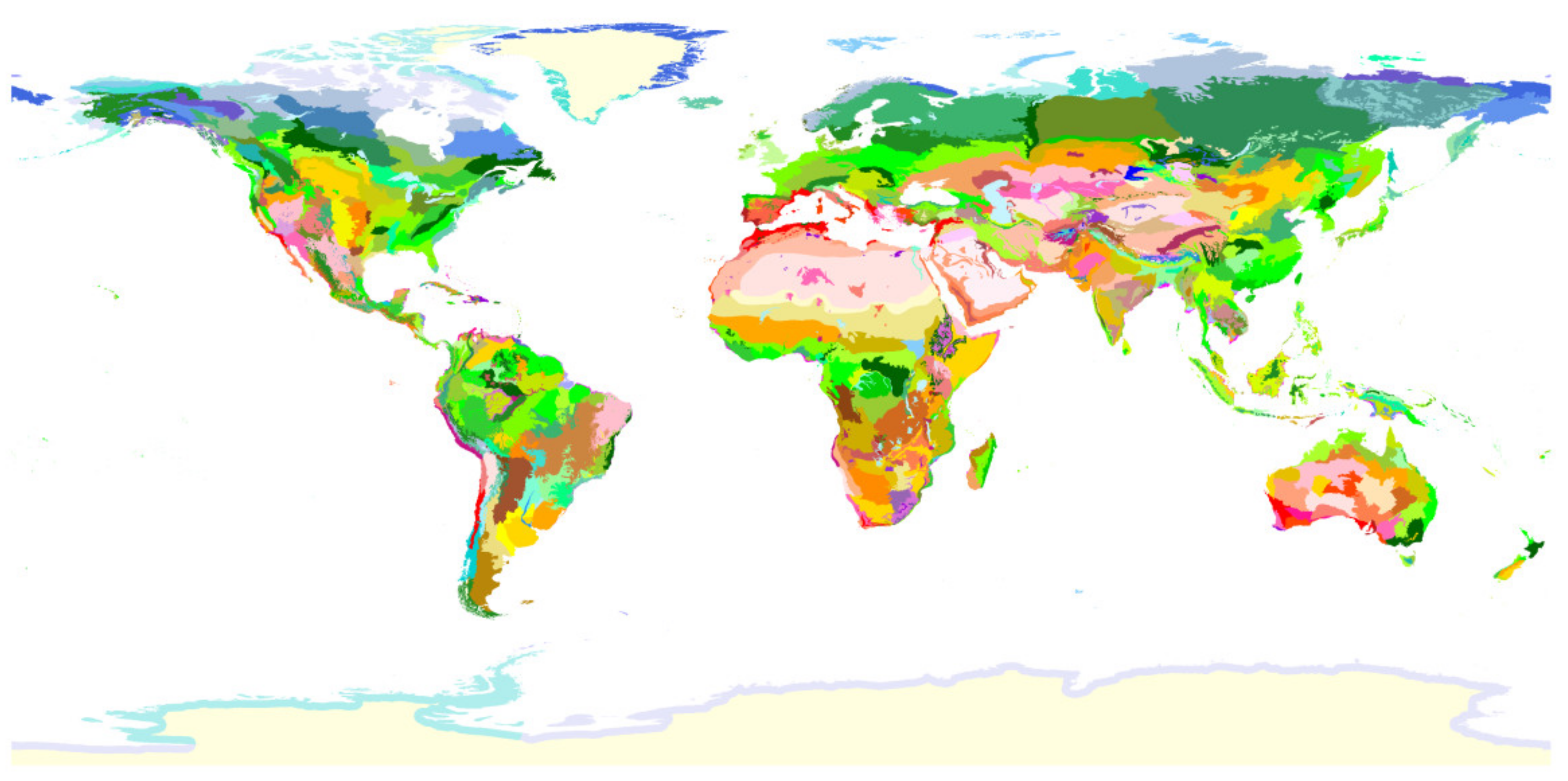
1.4. Concept of Eco-Geographical Zoning to Aid in Spurious Change Detection
1.5. Concept of Crowdsourced Data Mining to Aid in Spurious Change Detection
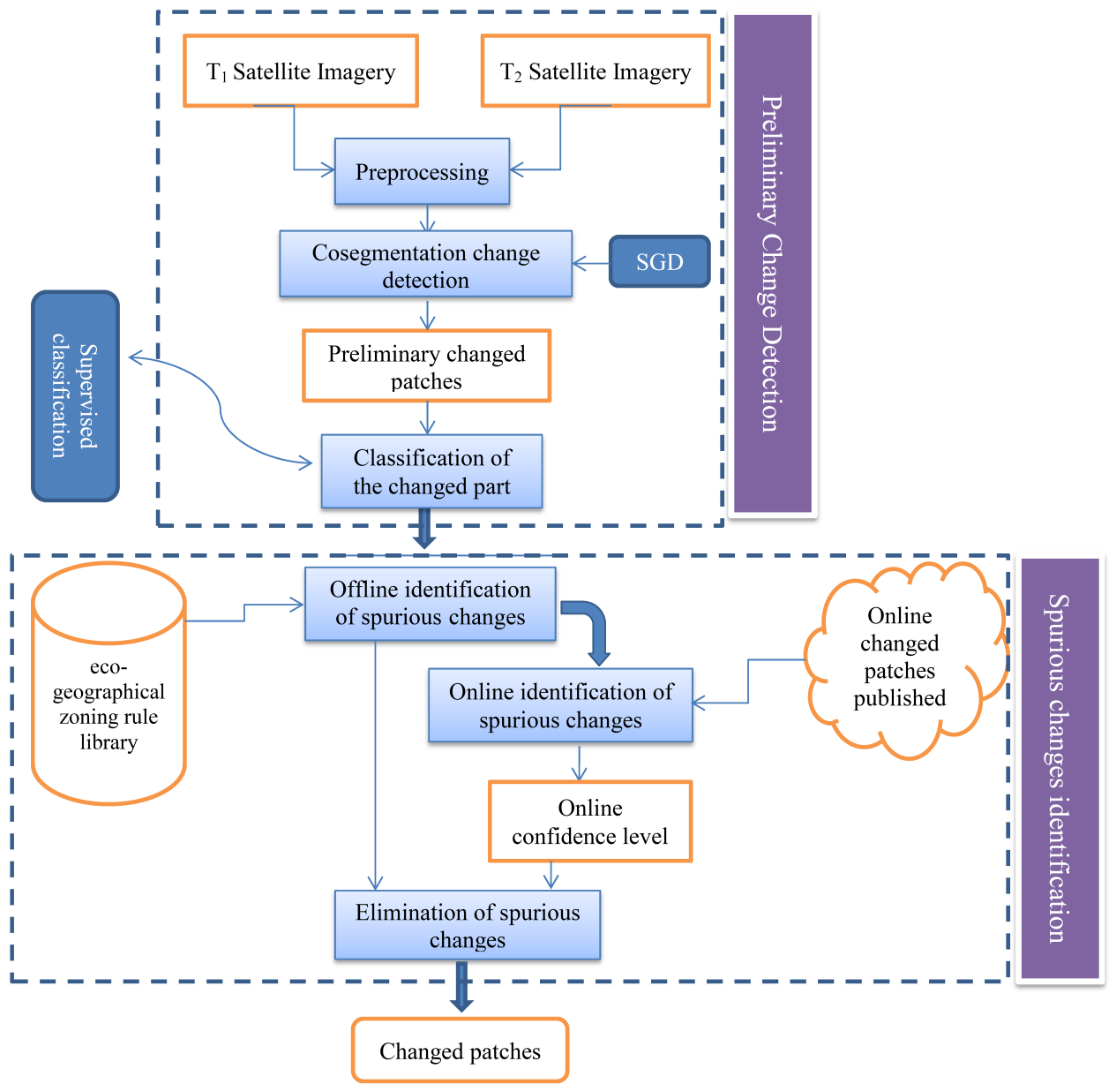
2. Method
2.1. Method Overview
2.2. Image Preprocessing and Change Detection
2.2.1. Preprocessing
- (1)
- Ortho correction: Ortho correction was carried out according to the Rational Polynomial Coefficients (RPC) file contained in the image download file and the corresponding Advanced Spaceborne Thermal Emission and Reflection Radiometer (ASTER) 30 m resolution DEM (Digital Elevation Model) of the area;
- (2)
- Radiometric calibration: The radiometric calibration coefficient of the GF-1 image was used to calibrate the image, and the image acquisition time, sensor type, aerosol mode, and other parameters for Fast Line-of-Sight Atmospheric Analysis of Spectral Hypercubes (FLAASH) atmospheric correction were inputted;
- (3)
- Geometric correction: The GF-1 WFV image has the characteristics of a wide coverage, large field of view, and complex geometric distortion. When using commercial software for image geometric correction, several local areas still appear to have deviations of a few pixels, resulting in an inability to achieve the accurate registration of two-phase images. For local geometric deformations, the conventional method is to use a large number of high-precision, evenly distributed control points to build a local correction model. Therefore, for GF-1 WFV images, the key to achieving a precise geometric correction is the acquisition of a large number of control points with high precision and a uniform distribution. In this study, the method of Shan et al. [34] was adopted. Based on a global mosaic image from the Landsat Thematic Mapper (TM), the hierarchical registration method was based on the Forstner operator and template matching. This method uses numerous high-precision, evenly distributed control points obtained by hierarchical matching to construct the Delaunay triangulation, which effectively solves the problem of geometric precision correction of GF-1 WFV images. The steps include GF-1 WFV image feature point extraction, hierarchical automatic image matching, control point homogenization, and triangulation correction. The registration error is less than 2 pixels.
2.2.2. Super Pixel Cosegmentation Change Detection
2.2.3. Change Patch Classification
2.2.4. Two-Phase Overlay Analysis
2.3. Eco-Geographical Zoning Rule Base
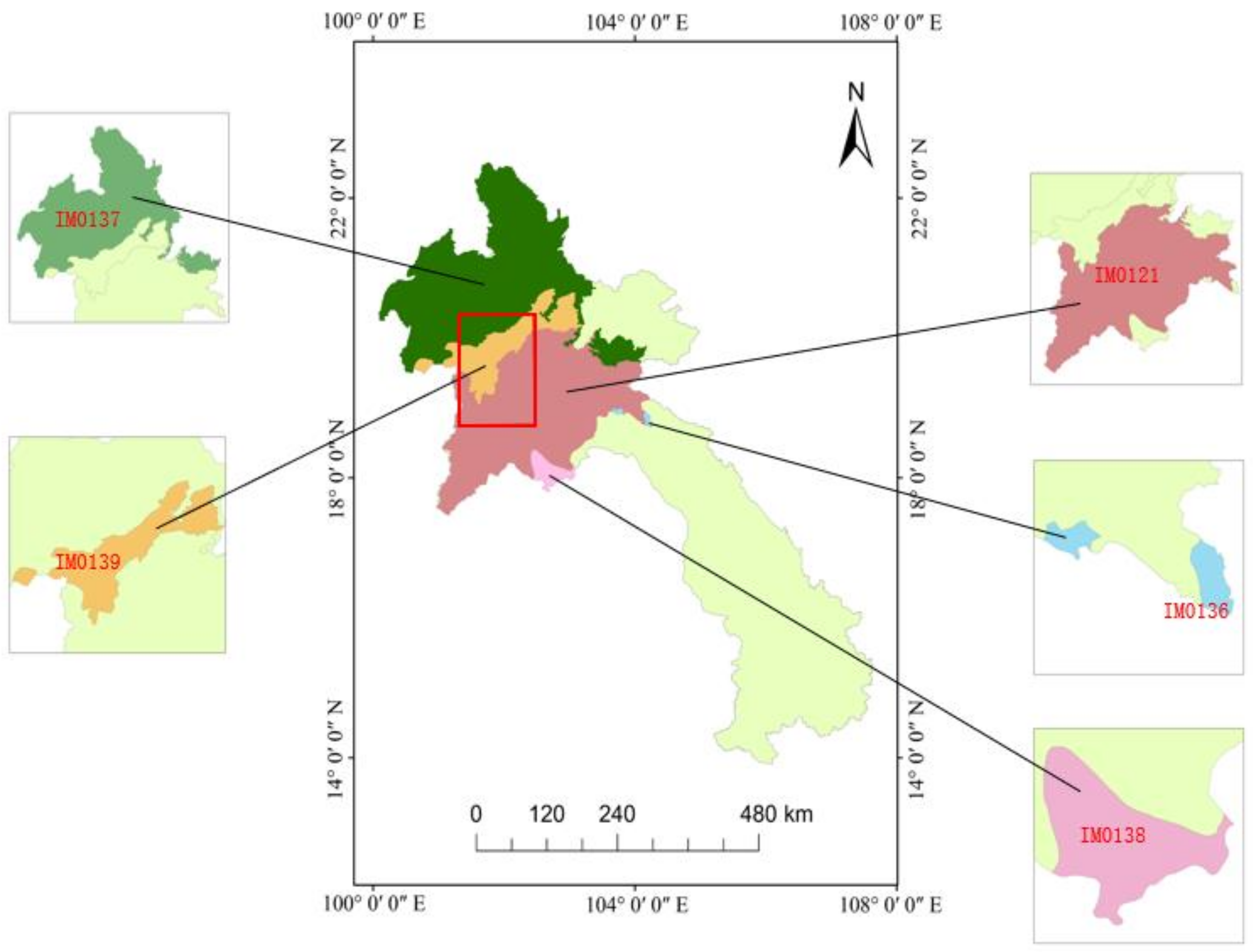
2.3.1. Eco-Geographical Zoning
2.3.2. Eco-Geographical Zoning Rule Base
Framework of Eco-Geographical Zoning Rule Base
- (1)
- Each eco-geographical zone is divided according to certain geographical attributes, and the information of different land types can be collected based on these different geographical attributes (such as elevation, slope, precipitation, and NDVI);
- (2)
- Different land cover types in each eco-geographical zone follow certain rules, and these rules can be extracted from the geographical attribute information collected on various categories.
Prior Knowledge Collection
2.4. Online Crowdsourced Spurious Change Tagging
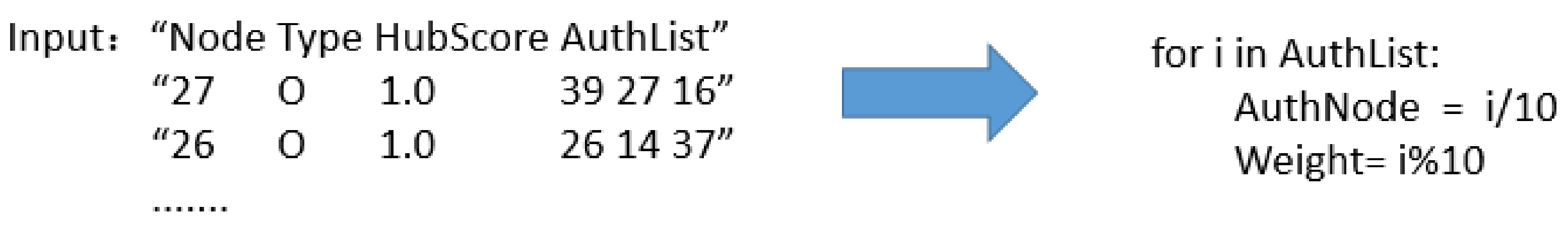
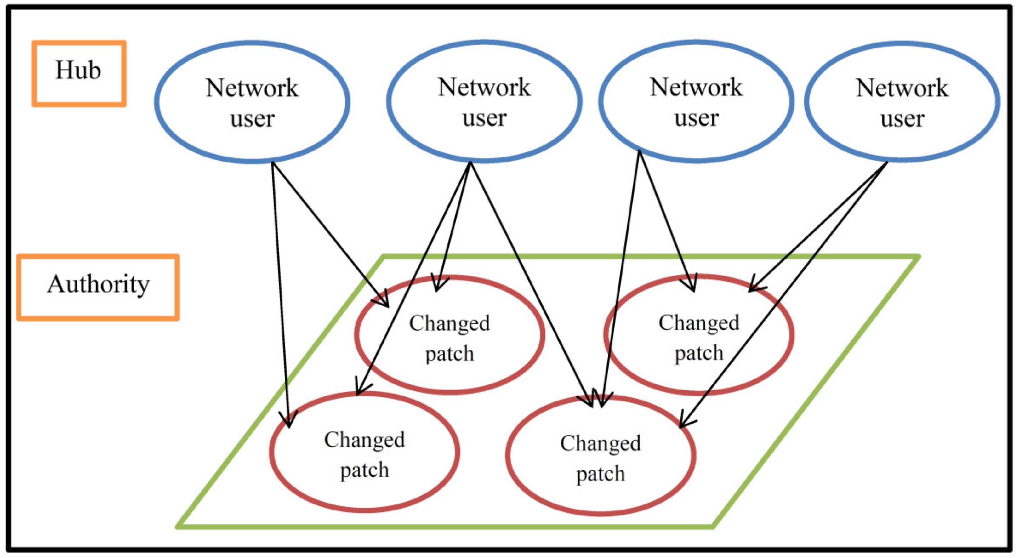
2.4.1. HITS Crowdsourced Data Mining
- (1)
- Calculate the authority value of the node, that is:
- (2)
- Normalize by:
- (3)
- The hub value of the node is calculated:
- (4)
- Normalize by:
- (1)
- is node ’s authority value:
- (2)
- After the standardization of , the following results are obtained:
- (3)
- is the hub value of node n:
- (4)
- After the standardization of , the following results are obtained:
2.4.2. Design of Online Crowdsourcing Spurious Change Detection Platform
- (1)
- Design and implementation of user-input collection module for crowdsourcing network:
- (2)
- Design and implementation of the spurious change detection module:
2.4.3. Screening Changed Patches for Online Crowdsourced Publishing
3. Data
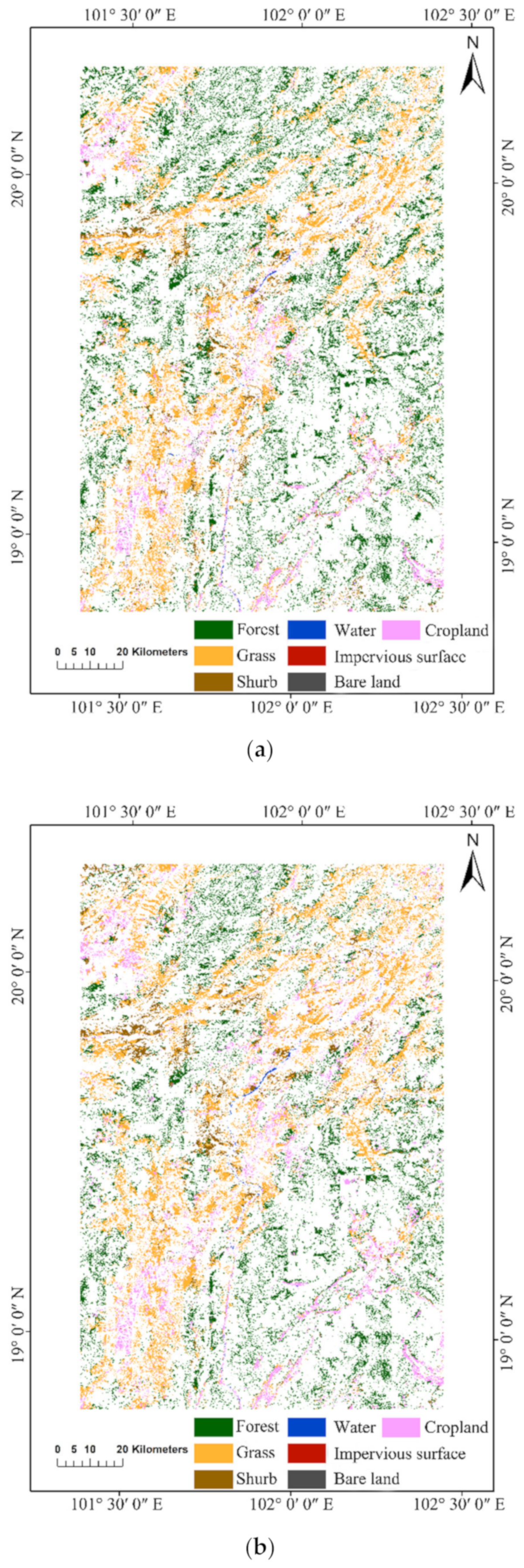
3.1. Study Area
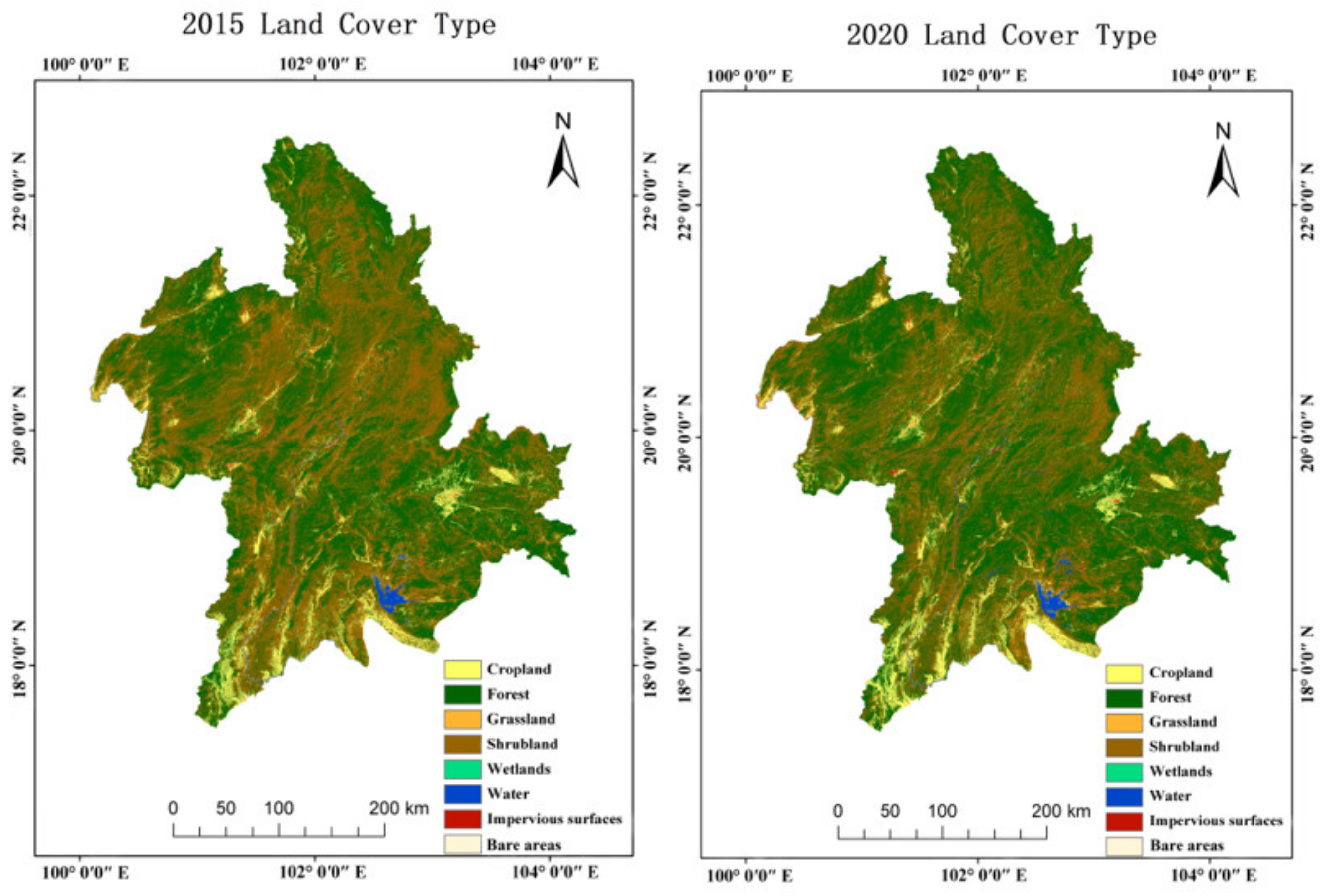
3.2. 2015 and 2020 GLC_FCS30 Products
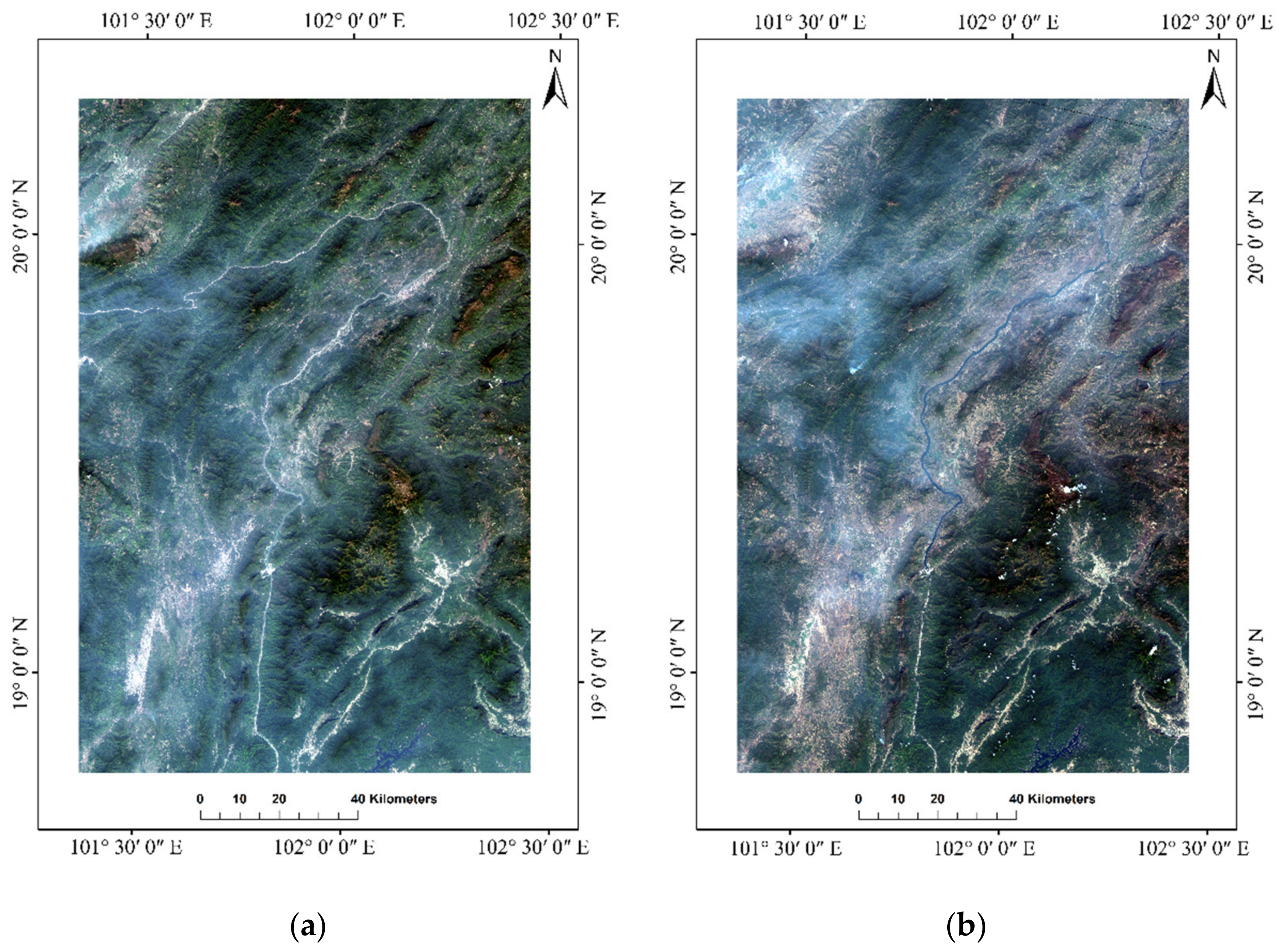
3.3. GF-1 WFV Image
4. Results
4.1. Change Detection
4.2. Result of Classification
4.3. Eco-Geographical Zoning Rule Base Spurious Change Detection Results
4.4. Crowdsourcing Online Spurious Change Tagging and Data Mining
4.5. Accuracy Assessment
5. Discussions
6. Conclusions
Author Contributions
Funding
Institutional Review Board Statement
Informed Consent Statement
Data Availability Statement
Conflicts of Interest
References
- Zhu, L.; Jia, T.; Shi, R. Global Surface Covering Product Update and Integration; Science Press: Beijing, China, 2020. (In Chinese) [Google Scholar]
- Chen, J.; Chen, J.; Liao, A. Remote Sensing Mapping of Global Land Cover; Science Press: Beijing, China, 2016. (In Chinese) [Google Scholar]
- Zhu, L.; Sun, Y.; Shi, R.M.; La, Y.X.; Peng, S. Exploiting Cosegmentation and Geo-Eco Zoning for Land Cover Product Updating. Photogramm. Eng. Remote Sens. 2019, 85, 597–611. [Google Scholar] [CrossRef]
- Zhang, L.; Wu, C. Current situation and Prospect of multi temporal remote sensing image change detection. J. Surv. Mapp. 2017, 46, 1447–1459. [Google Scholar]
- Chen, J.; Lu, M.; Chen, X.; Chen, J.; Chen, L. A spectral gradient difference based approach for land cover change detection. ISPRS J. Photogramm. Remote Sens. 2013, 85, 1–12. [Google Scholar] [CrossRef]
- Hu, Y.; Dong, Y. An automatic approach for land-change detection and land updates based on integrated NDVI timing analysis and the CVAPS method with GEE support. ISPRS J. Photogramm. Remote Sens. 2018, 146, 347–359. [Google Scholar] [CrossRef]
- Li, W.; Zhang, C.; Willig, M.R.; Dey, D.K.; Wang, G.; You, L. Bayesian Markov Chain Random Field Cosimulation for Improving Land Cover Classification Accuracy. Math. Geosci. 2015, 47, 123–148. [Google Scholar] [CrossRef]
- Giri, C.P. Remote Sensing of Land Use and Land Cover: Principles and Applications; CRC Press: Boca Raton, FL, USA, 2012. [Google Scholar]
- Mora, B.; Tsendbazar, N.E.; Herold, M.; Arino, O. Global Land Cover Mapping: Current Status and Future Trends; Springer Press: Dordrecht, The Netherlands, 2014. [Google Scholar]
- Chen, J.; Chen, J.; Liao, A.; Cao, X.; Chen, L.; Chen, X.; He, C.; Han, G.; Peng, S.; Lu, M.; et al. Global land cover mapping at 30 m resolution: A POK-based operational approach. ISPRS J. Photogramm. Remote Sens. 2015, 103, 7–27. [Google Scholar] [CrossRef] [Green Version]
- Liu, T.; Chen, X.; Dong, Q.; Cao, X.; Chen, J. Application of deep learning in product classification accuracy optimization of globeland30-2010. Remote Sens. Technol. Appl. 2019, 34, 3–11. (In Chinese) [Google Scholar]
- You, Y.; Cao, J.; Zhou, W. A Survey of Change Detection Methods Based on Remote Sensing Images for Multi-Source and Multi-Objective Scenarios. Remote Sens. 2020, 12, 2460. [Google Scholar] [CrossRef]
- Sood, V.; Gusain, H.S.; Gupta, S.; Singh, S. Topographically derived subpixel-based change detection for monitoring changes over rugged terrain Himalayas using AWiFS data. J. Mt. Sci. 2021, 18, 126–140. [Google Scholar] [CrossRef]
- Zhou, J.; Yu, B.; Qin, J. Multi-Level Spatial Analysis for Change Detection of Urban Vegetation at Individual Tree Scale. Remote Sens. 2014, 6, 9086–9103. [Google Scholar] [CrossRef] [Green Version]
- Lu, M.; Chen, J.; Tang, H.; Rao, Y.; Yang, P.; Wu, W. Land cover change detection by integrating object-based data blending model of Landsat and MODIS. Remote Sens. Environ. 2016, 184, 374–386. [Google Scholar] [CrossRef]
- Wang, L.; Luo, Y.; Zhang, X.; Ma, Q.; Kari, H.; Jia, L. Research progress on Application of remote sensing technology in forest pest monitoring. World For. Res. 2008, 21, 37–43. [Google Scholar]
- Yan, D. Extraction of Inland Surface Water with Different Turbidity Based on Landsat Series Remote Sensing Images. Master’s Thesis, Northwestern University, Xi’an, China, 2004. (In Chinese). [Google Scholar]
- Lv, Z.Y.; Liu, T.F.; Zhang, P.; Benediktsson, J.A.; Lei, T.; Zhang, X. Novel Adaptive Histogram Trend Similarity Approach for Land Cover Change Detection by Using Bitemporal Very-High-Resolution Remote Sensing Images. IEEE Trans. Geosci. Remote Sens. 2019, 57, 9554–9574. [Google Scholar] [CrossRef]
- Liu, B.; Chen, J.; Chen, J.; Zhang, W. Land Cover Change Detection Using Multiple Shape Parameters of Spectral and NDVI Curves. Remote Sens. 2018, 10, 1251. [Google Scholar] [CrossRef] [Green Version]
- European Space Agency. CCI-LC Product User Guide; UCL-Geomatics: Louvain-la-Neuve, Belgium, 2017. [Google Scholar]
- Herbertson, A.J. The Major Natural Regions: An Essay in Systematic Geography. Geogr. J. 1905, 25, 300–310. [Google Scholar] [CrossRef]
- Carver, S.; Evans, A.; Kingston, R.; Turton, I. Public participation, GIS, and cyberdemocracy: Evaluating on-line spatial decision support systems. Environ. Plan. B Plan. Des. 2001, 28, 907–921. [Google Scholar] [CrossRef] [Green Version]
- Hudson-Smith, A.; Batty, M.; Crooks, A.; Milton, R. Mapping for the Masses: Accessing web 2.0 through crowdsourcing. Soc. Sci. Comput. Rev. 2009, 27, 524–538. [Google Scholar] [CrossRef]
- Li, D.; Qian, X. On data management of spontaneous geographic information. J. Wuhan Univ. 2010, 35, 379–383. (In Chinese) [Google Scholar]
- Goodchild, M.F.; Glennon, J.A. Crowdsourcing geographic information for disaster response: A research frontier. Int. J. Digit. Earth 2010, 3, 231–241. [Google Scholar] [CrossRef]
- Jia, T.; Yu, X.; Shi, W.; Liu, X.; Li, X.; Xu, Y. Detecting the regional delineation from a network of social media user interactions with spatial constraint: A case study of Shenzhen, China. Phys. A Stat. Mech. Appl. 2019, 531, 121719. [Google Scholar] [CrossRef]
- Haklay, M. Citizen Science and Volunteered Geographic Information: Overview and Typology of Participation; Springer: Boston, MA, USA, 2013. [Google Scholar] [CrossRef]
- Li, D. Looking forward to geospatial informatics in the era of big data. J. Surv. Mapp. 2016, 45, 379–384. [Google Scholar]
- Clark, M.L.; Mitchell, A.T. Virtual Interpretation of Earth Web-Interface Tool (VIEW-IT) for Collecting Land-Use/Land-Cover Reference Data. Remote Sens. 2011, 3, 601–620. [Google Scholar] [CrossRef] [Green Version]
- See, L.; Dmitry, S.; Myroslava, L.; Ian, M.; Steffen, F.; Alexis, C.; Christoph, P.; Christian, S.; Zhao, Y.Y.; Victor, M. Building a hybrid land cover map with crowdsourcing and geographically weighted regression—ScienceDirect. ISPRS J. Photogramm. Remote Sens. 2015, 103, 48–56. [Google Scholar] [CrossRef] [Green Version]
- Schepaschenko, D.; See, L.; Lesiv, M.; McCallum, I.; Fritz, S.; Salk, C.; Moltchanova, E.; Perger, C.; Shchepashchenko, M.; Shvidenko, A.; et al. Development of a global hybrid forest mask through the synergy of remote sensing, crowdsourcing and FAO statistics. Remote Sens. Environ. 2015, 162, 208–220. [Google Scholar] [CrossRef]
- Xing, H.; Meng, Y.; Hou, D.; Xu, H.; Liu, J. A Land-Cover Classification Method Using Point of Interest. Geomat. Inf. Sci. Wuhan Univ. 2019, 44, 758–764. [Google Scholar]
- Fan, W.; Wu, C.; Jin, W. Improving Impervious Surface Estimation by Using Remote Sensed Imagery Combined With Open Street Map Points-of-Interest (POI) Data. IEEE J. Sel. Top. Appl. Earth Obs. Remote Sens. 2019, 12, 4265–4274. [Google Scholar] [CrossRef]
- Shan, X.J.; Tang, P.; Hu, C.M.; Tang, L.; Zheng, K. Automatic geometric precise correction technology and system based on hierarchical image matching for HJ-1A/B CCD images. J. Remote Sens. 2014, 18, 254–266. [Google Scholar]
- Rother, C.; Minka, T.; Blake, A.; Kolmogorov, V. Cosegmentation of Image Pairs by Histogram Matching—Incorporating a Global Constraint into MRFs. In Proceedings of the 2006 IEEE Computer Society Conference on Computer Vision and Pattern Recognition (CVPR’06), New York, NY, USA, 17–22 June 2006. [Google Scholar]
- Zhu, L.; Zhang, J.; Sun, Y. Remote Sensing Image Change Detection Using Superpixel Cosegmentation. Information 2021, 12, 94. [Google Scholar] [CrossRef]
- Olson, D.M.; Dinerstein, E.; Wikramanayake, E.D.; Burgess, N.D.; Powell, G.V.; Underwood, E.C.; D’amico, J.A.; Itoua, I.; Strand, H.E.; Morrison, J.C.; et al. Terrestrial Ecoregions of the World: A New Map of Life on Earth. BioScience 2001, 51, 933–938. [Google Scholar] [CrossRef]
- Jon, M.K. Authoritative sources in a hyperlinked environment. J. ACM 1999, 46, 604–632. [Google Scholar]
- Zhang, X.; Liu, L.; Chen, X.; Gao, Y.; Xie, S.; Mi, J. GLC_FCS30: Global land-cover product with fine classification system at 30 m using time-series Landsat imagery. Earth Syst. Sci. Data 2021, 13, 2753–2776. [Google Scholar] [CrossRef]
- Benedek, C.; Szirányi, T. Change Detection in Optical Aerial Images by a Multi-Layer Conditional Mixed Markov Model. IEEE Trans. Geosci. Remote Sens. 2009, 47, 3416–3430. [Google Scholar] [CrossRef] [Green Version]


| Multispectral Cameras | Band Number | Wave Range (μm) | Spatial Resolution (m) | Width (km) | Sway Ability | Revisit Period (Days) |
|---|---|---|---|---|---|---|
| 6 | 0.45–0.52 | 16 | 800 (four-camera combination) | ±35° | 2 | |
| 7 | 0.52–0.59 | |||||
| 8 | 0.63–0.69 | |||||
| 9 | 0.77–0.89 |
| Code | Land Cover Class | Definition |
|---|---|---|
| 010 | Cultivated land | Refers to land used for cultivating crops. Paddy fields, irrigated upland, rainfed upland, vegetable land, cultivated pastures, and greenhouse land are included in this category. |
| 020 | Forests | Refers to land covered with trees, the top density of which occupies over 30%. Deciduous broadleaf forests, evergreen broadleaf forests, deciduous coniferous forests, evergreen coniferous forests, mixed forest and sparse woodlands, the top density of which covers 10–30%, are included in this category. |
| 030 | Shrublands | Refers to land covered with shrubs areas with a cover density over 30%. Mountain shrubs, deciduous and evergreen shrubs, and desert jungles in desert areas with a cover density over 10% are included in this category. |
| 040 | Grasslands | Refers to land covered by herbaceous vegetation. This includes all kinds of grasslands with more than 10% grass coverage, including shrub grasslands dominated by grazing and sparse forest grasslands with less than 10% forest coverage. |
| 050 | Wetlands | Refers to the junctions of land and water areas, which are constantly covered by biogas or hygrophyte plants and shallow water or wet soils. Inland marshes, lake marshes, river floodplain wetlands, forest/shrub wetlands, peat bogs, mangroves, salt marshes, etc., are included in this category. |
| 060 | Water bodies | Refers to liquid water-covered regions in land areas. Rivers, lakes, reservoirs, pit ponds, etc., are included in this category. |
| 070 | Artificial surfaces | Refers to surfaces formed by human-made activities. All kinds of habitation in urban and rural areas, industrial and mining areas, transportation facilities, etc., are included in this category, whereas interior contiguous green land and water bodies are not included. |
| 080 | Bare land | Refers to naturally covered land with a vegetation cover density lower than 10%. Deserts, sand, gravel ground, bare rocks, saline and alkaline land, etc., are included in this category. |
| 090 | Permanent snow and ice | Refers to land covered by permanent snow, glaciers, and icecaps. |
| 100 | Tundra | Refers to land covered by lichen, moss, hardy perennial herbs and shrubs in cold and high mountain areas. Shrub tundra, grass tundra, wet tundra, alpine tundra, barren tundra, etc., are included in this category. |
| Phase 2 | Cropland | Forests | Grass | Shrubs | Wetlands | Water | Sum | |
|---|---|---|---|---|---|---|---|---|
| Phase 1 | ||||||||
| Cropland | N11 | N12 | N13 | N14 | N15 | N16 | ||
| Forests | N21 | N22 | N23 | N24 | N25 | N26 | ||
| Grass | N31 | N32 | N33 | N34 | N35 | N36 | ||
| Shrubs | N41 | N42 | N43 | N44 | N45 | N46 | ||
| Wetlands | N51 | N52 | N53 | N54 | N55 | N56 | ||
| Water | N61 | N62 | N63 | N64 | N65 | N66 | ||
| Sum | ||||||||
| Land Cover | Cropland | Forests | Grass | Shrubs | Wetlands | Water | Sum |
|---|---|---|---|---|---|---|---|
| Cropland | P11 | P12 | P13 | P14 | P15 | P16 | 1 |
| Forests | P21 | P22 | P23 | P24 | P25 | P26 | 1 |
| Grass | P31 | P32 | P33 | P34 | P35 | P36 | 1 |
| Shrubs | P41 | P42 | P43 | P44 | P45 | P46 | 1 |
| Wetlands | P51 | P52 | P53 | P54 | P55 | P56 | 1 |
| Water | P61 | P62 | P63 | P64 | P65 | P66 | 1 |
| Sum | 1 | 1 | 1 | 1 | 1 | 1 |
| Time | 2015 | 2020 | |||
|---|---|---|---|---|---|
| Land Cover | Pixel Count | Proportion | Pixel Count | Proportion | |
| Cropland | 1,369,323 | 5.70% | 1,468,986 | 6.12% | |
| Forests | 10,515,595 | 43.79% | 12,025,140 | 50.12% | |
| Grass | 15,723 | 0.07% | 10,602 | 0.04% | |
| Shrubs | 11,927,722 | 49.67% | 10,182,737 | 42.44% | |
| Wetlands | 11,560 | 0.05% | 3129 | 0.01% | |
| Water | 119,395 | 0.49% | 163,235 | 0.68% | |
| Impervious surfaces | 55,088 | 0.23% | 140,651 | 0.59% | |
| IM0121 | ||||||||
| Land Cover | Cropland | Forest | Grass | Shrub | Wetland | Water | Artificial | |
| Cropland | 0.655662 | 0.138724 | 0.000083 | 0.172982 | 0.000358 | 0.011288 | 0.020905 | |
| Forest | 0.025709 | 0.797330 | 0.000019 | 0.174539 | 0.000116 | 0.001765 | 0.000522 | |
| Grass | 0.518326 | 0.292829 | 0.001112 | 0.037833 | 0.006076 | 0.128777 | 0.015047 | |
| Shrub | 0.061172 | 0.273834 | 0.000016 | 0.662740 | 0.000148 | 0.000636 | 0.001454 | |
| Wetland | 0.528367 | 0.172955 | 0.000632 | 0.153999 | 0.057118 | 0.066415 | 0.020514 | |
| Water | 0.068448 | 0.006729 | 0.000153 | 0.003885 | 0.001945 | 0.914736 | 0.004104 | |
| Artificial | 0.297608 | 0.013116 | 0.000000 | 0.014344 | 0.000054 | 0.007900 | 0.666979 | |
| IM0137 | ||||||||
| Land Cover | Cropland | Forest | Grass | Shrub | Wetland | Water | Artificial | Bare Land |
| Cropland | 0.501647 | 0.178256 | 0.005283 | 0.261301 | 0.000155 | 0.005802 | 0.047551 | 0.000006 |
| Forest | 0.008681 | 0.829920 | 0.001236 | 0.159641 | 0.000025 | 0.000226 | 0.000271 | 0.000000 |
| Grass | 0.160823 | 0.580679 | 0.059788 | 0.121092 | 0.000208 | 0.034025 | 0.043385 | 0.000000 |
| Shrub | 0.037345 | 0.281683 | 0.001239 | 0.678366 | 0.000019 | 0.000279 | 0.001068 | 0.000000 |
| Wetland | 0.445588 | 0.208367 | 0.001345 | 0.137880 | 0.003228 | 0.015268 | 0.188324 | 0.000000 |
| Water | 0.112686 | 0.069924 | 0.032684 | 0.036265 | 0.004447 | 0.729387 | 0.014606 | 0.000000 |
| Artificial | 0.190790 | 0.005327 | 0.005062 | 0.007981 | 0.000038 | 0.001232 | 0.789494 | 0.000076 |
| IM0139 | ||||||||
| Land Cover | Cropland | Forest | Grass | Shrub | Wetland | Water | Artificial | |
| Cropland | 0.489749 | 0.203831 | 0.002754 | 0.211230 | 0.000668 | 0.026297 | 0.065472 | |
| Forest | 0.013997 | 0.783616 | 0.000702 | 0.199963 | 0.000053 | 0.000365 | 0.001304 | |
| Grass | 0.252498 | 0.222519 | 0.022801 | 0.054469 | 0.005630 | 0.281070 | 0.161013 | |
| Shrub | 0.038376 | 0.240848 | 0.000739 | 0.717184 | 0.000066 | 0.000657 | 0.002129 | |
| Wetland | 0.323329 | 0.269231 | 0.000899 | 0.188893 | 0.061467 | 0.087527 | 0.068656 | |
| Water | 0.050101 | 0.018540 | 0.005219 | 0.005432 | 0.001748 | 0.904035 | 0.014924 | |
| Artificial | 0.189507 | 0.021239 | 0.000378 | 0.012762 | 0.000113 | 0.012064 | 0.763937 | |
| Ecological Divisions | Rule (A→B) | Confidence Level |
|---|---|---|
| IM01 | Water–forest | 0.8 |
| Artificial surface–forest | 0.9 | |
| Bare land–forest | 0.7 | |
| Cropland– forest | 0.8 |
| Eco-Geographical Zone | Source of Rules | Types of Land Cover Transformation | Number of Potential Spurious Changed Patches |
|---|---|---|---|
| IM01 | From an interpreter | Water–forest | 11 |
| Artificial surface–forest | 4 | ||
| Bare land–forest | 252 | ||
| Cropland–forest | 2056 | ||
| Changed patches with the same type of land cover before and after transformation | Cropland–cropland | 12,511 | |
| Forest–forest | 33,609 | ||
| Shrub–shrub | 23,464 | ||
| Grass–grass | 8682 | ||
| Water–water | 707 | ||
| Artificial surface–artificial surface | 764 | ||
| Bare land–bare land | 211 | ||
| IM0121 | Statistics from land cover products—low-probability events | Cropland–grass | 960 |
| Forest–grass | 3634 | ||
| Shrub–grass | 1679 | ||
| Artificial surface–grass | 9 | ||
| IM0137 | Cropland–bare land | 3 | |
| Forest–bare land | 81 | ||
| Grass–bare land | 31 | ||
| Shrub–bare land | 29 | ||
| Water–bare land | 1 | ||
| Sum | 88,698 | ||
| Change Patch Serial Number | Authority Value |
|---|---|
| 13317 | 1 |
| 14779 | 1 |
| 13643 | 1 |
| 3456 | 1 |
| 9166 | 1.4142 |
| 14713 | 1 |
| 7041 | 1 |
| 14882 | 1 |
| 667 | 1 |
| 7020 | 1.4108 |
| 8077 | 1 |
| 1325 | 1 |
| 3517 | 1.4142 |
| 3877 | 1 |
| 7988 | 1 |
| 204 | 1 |
| 956 | 1 |
| 1 | 1 |
| 13310 | 1 |
| 3706 | 1.4 |
| 3436 | 1.022 |
| 12540 | 1 |
| T2\T1 | Changed | Unchanged | Sum |
|---|---|---|---|
| Changed | 113 | 195 | 308 |
| Unchanged | 0 | 278 | 278 |
| Sum | 113 | 473 | 586 |
| Overall Accuracy | 66.72% | ||
| KIA | 0.3548 |
| T2\T1 | Changed | Unchanged | Sum |
|---|---|---|---|
| Changed | 99 | 41 | 140 |
| Unchanged | 14 | 432 | 446 |
| Sum | 113 | 473 | 586 |
| Overall Accuracy | 90.61% | ||
| KIA | 0.7236 |
Publisher’s Note: MDPI stays neutral with regard to jurisdictional claims in published maps and institutional affiliations. |
© 2021 by the authors. Licensee MDPI, Basel, Switzerland. This article is an open access article distributed under the terms and conditions of the Creative Commons Attribution (CC BY) license (https://creativecommons.org/licenses/by/4.0/).
Share and Cite
Zhu, L.; Gao, D.; Jia, T.; Zhang, J. Using Eco-Geographical Zoning Data and Crowdsourcing to Improve the Detection of Spurious Land Cover Changes. Remote Sens. 2021, 13, 3244. https://doi.org/10.3390/rs13163244
Zhu L, Gao D, Jia T, Zhang J. Using Eco-Geographical Zoning Data and Crowdsourcing to Improve the Detection of Spurious Land Cover Changes. Remote Sensing. 2021; 13(16):3244. https://doi.org/10.3390/rs13163244
Chicago/Turabian StyleZhu, Ling, Dejun Gao, Tao Jia, and Jingyi Zhang. 2021. "Using Eco-Geographical Zoning Data and Crowdsourcing to Improve the Detection of Spurious Land Cover Changes" Remote Sensing 13, no. 16: 3244. https://doi.org/10.3390/rs13163244
APA StyleZhu, L., Gao, D., Jia, T., & Zhang, J. (2021). Using Eco-Geographical Zoning Data and Crowdsourcing to Improve the Detection of Spurious Land Cover Changes. Remote Sensing, 13(16), 3244. https://doi.org/10.3390/rs13163244