
Individual Tree Detection in Urban ALS Point Clouds with 3D Convolutional Networks


Abstract
:1. Introduction
2. Related Work
2.1. Individual Tree Detection in (Urban) Forests
2.2. MLS and Other Data Sources
2.3. Deep Learning for Individual Tree Detection
2.4. Three-Dimensional Deep Learning
2.5. Ground Truth Data
3. Materials and Methods
3.1. Methodology
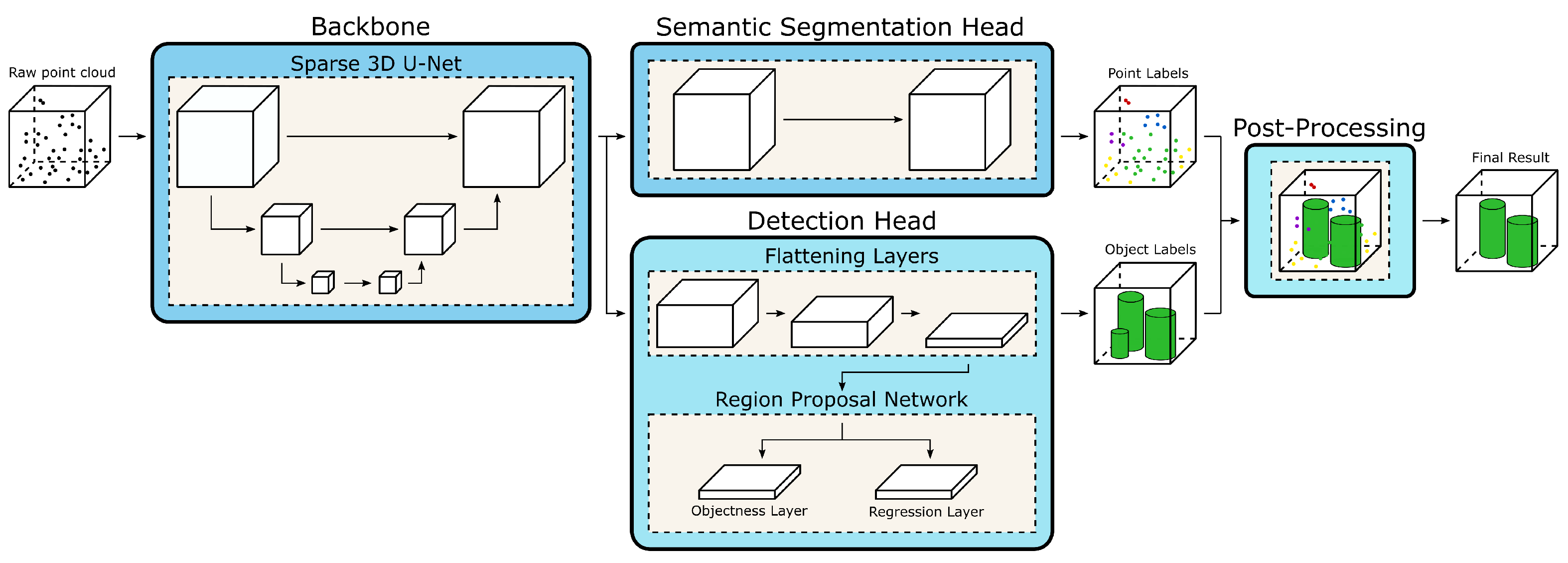
3.1.1. Architecture
3.1.2. Training
3.1.3. Inference
3.1.4. Region Growing
3.2. Data
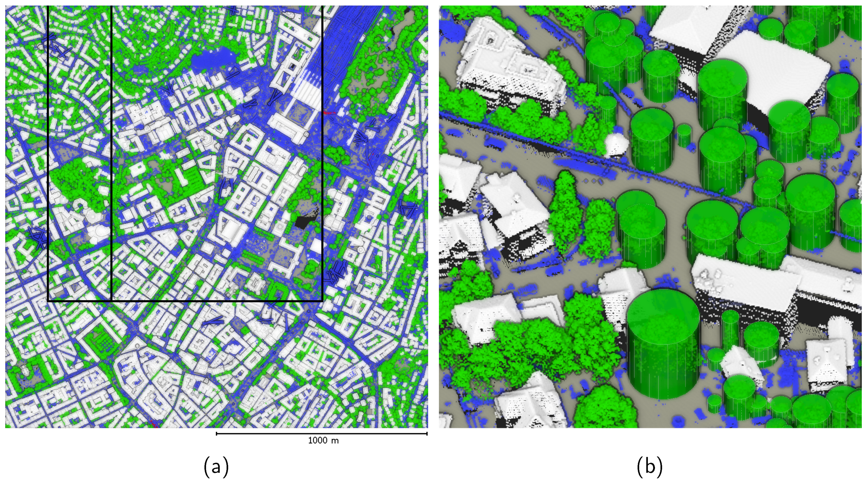
3.2.1. Study Area
3.2.2. Ground Truth Generation
3.3. Baselines
3.3.1. nDSM Segmentation
3.3.2. Two-Dimensional Object Detection Networks
4. Results
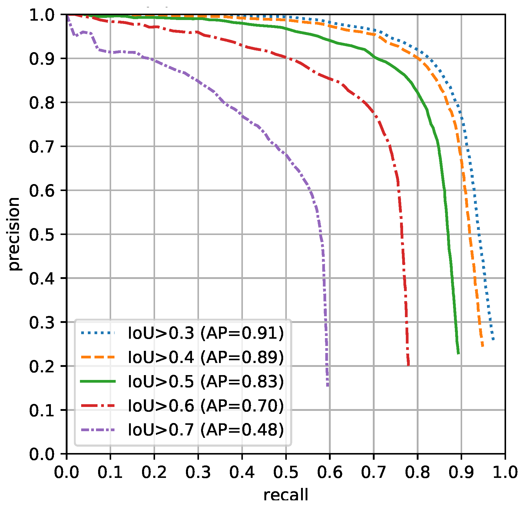
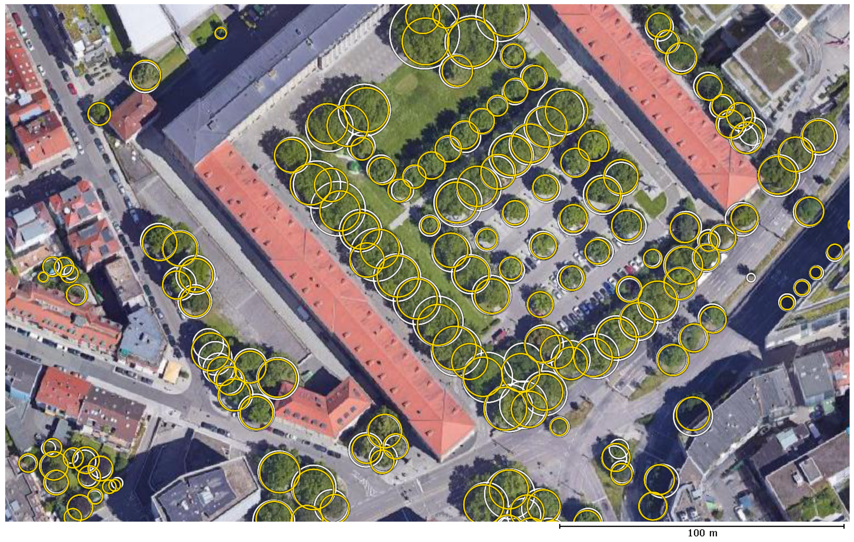
4.1. Individual Tree Detection
4.2. Stem Precision and Recall
4.3. Tree Canopy Cover
4.4. Ablations and Things That Did Not Work
4.4.1. Pre-Training
4.4.2. Weighted Shape Regression and Loss Function
4.4.3. Data Augmentation
4.4.4. Shape Regression
4.4.5. RGB Input Features
4.4.6. Three-Dimensional vs. Two-Dimensional Backbone
5. Discussion
6. Conclusions
Author Contributions
Funding
Acknowledgments
Conflicts of Interest
References
- Nowak, D.J.; Crane, D.E.; Stevens, J.C. Air pollution removal by urban trees and shrubs in the United States. Urban For. Urban Green. 2006, 4, 115–123. [Google Scholar] [CrossRef]
- Weng, Q.; Lu, D.; Schubring, J. Estimation of land surface temperature–vegetation abundance relationship for urban heat island studies. Remote Sens. Environ. 2004, 89, 467–483. [Google Scholar] [CrossRef]
- Chen, X.L.; Zhao, H.M.; Li, P.X.; Yin, Z.Y. Remote sensing image-based analysis of the relationship between urban heat island and land use/cover changes. Remote Sens. Environ. 2006, 104, 133–146. [Google Scholar] [CrossRef]
- Kurn, D.M.; Bretz, S.E.; Huang, B.; Akbari, H. The Potential for Reducing Urban Air Temperatures and Energy Consumption through Vegetative Cooling; Technical report; Lawrence Berkeley Laboratory: Berkeley, CA, USA, 1994. [CrossRef] [Green Version]
- Huang, Y.J.; Akbari, H.; Taha, H. The wind-shielding and shading effects of trees on residential heating and cooling requirements. In Proceedings of the ASHRAE Winter Conference, Atlanta, GA, USA, 11–14 February 1990; pp. 11–14. [Google Scholar]
- McPherson, E.G.; Simpson, J.R. Potential energy savings in buildings by an urban tree planting programme in California. Urban For. Urban Green. 2003, 2, 73–86. [Google Scholar] [CrossRef]
- Pesola, L.; Cheng, X.; Sanesi, G.; Colangelo, G.; Elia, M.; Lafortezza, R. Linking above-ground biomass and biodiversity to stand development in urban forest areas: A case study in Northern Italy. Landsc. Urban Plan. 2017, 157, 90–97. [Google Scholar] [CrossRef]
- Nielsen, A.B.; Östberg, J.; Delshammar, T. Review of urban tree inventory methods used to collect data at single-tree level. Arboric. Urban For. 2014, 40, 96–111. [Google Scholar] [CrossRef]
- Bardekjian, A.; Kenney, A.R.M. Trends in Canada’s Urban Forests. In Trees Canada—Arbres Canada and Canadian Urban Forest Network—Réseau Canadien de la Floret Urbaine. 2016. Available online: https://treecanada.ca/wp-content/uploads/2017/10/Article-1-EN-CUFN-Trends-in-Canada%E2%80%99s-Urban-Forests.pdf (accessed on 9 February 2021).
- Hauer, R.J.; Peterson, W.D. Municipal Tree Care and Management in the United States: A 2014 Urban & Community Forestry Census of Tree Activities; Special Publication 16-1; College of Natural Resources, University of Wisconsin—Stevens Point: Madison, WI, USA, 2016. [Google Scholar]
- Östberg, J.; Wiström, B.; Randrup, T.B. The state and use of municipal tree inventories in Swedish municipalities—Results from a national survey. Urban Ecosyst. 2018, 21, 467–477. [Google Scholar] [CrossRef] [Green Version]
- McPherson, E.G. Structure and sustainability of Sacramento’s urban forest. J. Arboric. 1998, 24, 174–190. [Google Scholar] [CrossRef]
- Cameron, R.W.; Blanuša, T.; Taylor, J.E.; Salisbury, A.; Halstead, A.J.; Henricot, B.; Thompson, K. The domestic garden—Its contribution to urban green infrastructure. Urban For. Urban Green. 2012, 11, 129–137. [Google Scholar] [CrossRef]
- Kelly, M. Urban trees and the green infrastructure agenda. In Trees, People and the Built Environment, Proceedings of the Urban Trees Research Conference, 13–14 April 2011; Johnston, M., Percival, G., Eds.; Forestry Commission: Macon, GA, USA, 2012; pp. 166–180. [Google Scholar]
- Li, X.; Chen, W.Y.; Sanesi, G.; Lafortezza, R. Remote Sensing in Urban Forestry: Recent Applications and Future Directions. Remote Sens. 2019, 11, 1144. [Google Scholar] [CrossRef] [Green Version]
- Casalegno, S.; Anderson, K.; Hancock, S.; Gaston, K.J. Improving models of urban greenspace: From vegetation surface cover to volumetric survey, using waveform laser scanning. Methods Ecol. Evol. 2017, 8, 1443–1452. [Google Scholar] [CrossRef] [Green Version]
- Strîmbu, V.F.; Strîmbu, B.M. A graph-based segmentation algorithm for tree crown extraction using airborne LiDAR data. ISPRS J. Photogramm. Remote Sens. 2015, 104, 30–43. [Google Scholar] [CrossRef] [Green Version]
- Kattenborn, T.; Leitloff, J.; Schiefer, F.; Hinz, S. Review on Convolutional Neural Networks (CNN) in vegetation remote sensing. ISPRS J. Photogramm. Remote Sens. 2021, 173, 24–49. [Google Scholar] [CrossRef]
- Schmohl, S.; Kölle, M.; Frolow, R.; Soergel, U. Towards Urban Tree Recognition in Airborne Point Clouds with Deep 3D Single-Shot Detectors. In Pattern Recognition. ICPR International Workshops and Challenges; Del Bimbo, A., Cucchiara, R., Sclaroff, S., Farinella, G.M., Mei, T., Bertini, M., Escalante, H.J., Vezzani, R., Eds.; Springer International Publishing: Cham, Switzerland, 2021; pp. 521–535. [Google Scholar]
- Kaartinen, H.; Hyyppä, J.; Yu, X.; Vastaranta, M.; Hyyppä, H.; Kukko, A.; Holopainen, M.; Heipke, C.; Hirschmugl, M.; Morsdorf, F.; et al. An International Comparison of Individual Tree Detection and Extraction Using Airborne Laser Scanning. Remote Sens. 2012, 4, 950–974. [Google Scholar] [CrossRef] [Green Version]
- Jakubowski, M.K.; Li, W.; Guo, Q.; Kelly, M. Delineating Individual Trees from Lidar Data: A Comparison of Vector- and Raster-based Segmentation Approaches. Remote Sens. 2013, 5, 4163–4186. [Google Scholar] [CrossRef] [Green Version]
- Eysn, L.; Hollaus, M.; Lindberg, E.; Berger, F.; Monnet, J.M.; Dalponte, M.; Kobal, M.; Pellegrini, M.; Lingua, E.; Mongus, D.; et al. A benchmark of lidar-based single tree detection methods using heterogeneous forest data from the alpine space. Forests 2015, 6, 1721–1747. [Google Scholar] [CrossRef] [Green Version]
- Wang, Y.; Hyyppä, J.; Liang, X.; Kaartinen, H.; Yu, X.; Lindberg, E.; Holmgren, J.; Qin, Y.; Mallet, C.; Ferraz, A.; et al. International Benchmarking of the Individual Tree Detection Methods for Modeling 3-D Canopy Structure for Silviculture and Forest Ecology Using Airborne Laser Scanning. IEEE Trans. Geosci. Remote Sens. 2016, 54, 5011–5027. [Google Scholar] [CrossRef] [Green Version]
- Hyyppä, J.; Kelle, O.; Lehikoinen, M.; Inkinen, M. A segmentation-based method to retrieve stem volume estimates from 3-D tree height models produced by laser scanners. IEEE Trans. Geosci. Remote Sens. 2001, 39, 969–975. [Google Scholar] [CrossRef]
- Hirschmugl, M.; Ofner, M.; Raggam, J.; Schardt, M. Single tree detection in very high resolution remote sensing data. Remote Sens. Environ. 2007, 110, 533–544. [Google Scholar] [CrossRef]
- Dalponte, M.; Coomes, D.A. Tree-centric mapping of forest carbon density from airborne laser scanning and hyperspectral data. Methods Ecol. Evol. 2016, 7, 1236–1245. [Google Scholar] [CrossRef] [Green Version]
- Pyysalo, U.; Hyyppä, H. Reconstructing Tree Crowns from Laser Scanner Data for Feature Extraction. Int. Arch. Photogramm. Remote Sens. 2002, 34, 218–221. [Google Scholar]
- Koch, B.; Heyder, U.; Weinacker, H. Detection of Individual Tree Crowns in Airborne Lidar Data. Photogramm. Eng. Remote Sens. 2006, 72, 357–363. [Google Scholar] [CrossRef] [Green Version]
- Zhao, K.; Popescu, S. Hierarchical Watershed Segmentation of Canopy Height Model for Multi-Scale Forest Inventory. ISPRS Workshop Laser Scanning 2007, 3, 436–441. [Google Scholar]
- Persson, A.; Holmgren, J.; Soderman, U. Detecting and Measuring Individual Trees Using an Airborne Laser Scanner. Photogramm. Eng. Remote Sens. 2002, 68, 925–932. [Google Scholar]
- Reitberger, J.; Heurich, M.; Krzystek, P.; Stilla, U. Single tree detection in forest areas with high-density LIDAR data. Int. Arch. Photogramm. Remote Sens. Spat. Inf. Sci. 2007, 36, 139–144. [Google Scholar]
- Li, W.; Guo, Q.; Jakubowski, M.K.; Kelly, M. A New Method for Segmenting Individual Trees from the Lidar Point Cloud. Photogramm. Eng. Remote Sens. 2012, 78, 75–84. [Google Scholar] [CrossRef] [Green Version]
- Lu, X.; Guo, Q.; Li, W.; Flanagan, J. A bottom-up approach to segment individual deciduous trees using leaf-off lidar point cloud data. ISPRS J. Photogramm. Remote Sens. 2014, 94, 1–12. [Google Scholar] [CrossRef]
- Ferraz, A.; Bretar, F.; Jacquemoud, S.; Gonçalves, G.; Pereira, L.; Tomé, M.; Soares, P. 3-D mapping of a multi-layered Mediterranean forest using ALS data. Remote Sens. Environ. 2012, 121, 210–223. [Google Scholar] [CrossRef]
- Dai, W.; Yang, B.; Dong, Z.; Shaker, A. A new method for 3D individual tree extraction using multispectral airborne LiDAR point clouds. ISPRS J. Photogramm. Remote Sens. 2018, 144, 400–411. [Google Scholar] [CrossRef]
- Xiao, W.; Zaforemska, A.; Smigaj, M.; Wang, Y.; Gaulton, R. Mean Shift Segmentation Assessment for Individual Forest Tree Delineation from Airborne Lidar Data. Remote Sens. 2019, 11, 1263. [Google Scholar] [CrossRef] [Green Version]
- Pollock, R.J. Model-based approach to automatically locating tree crowns in high spatial resolution images. In Image and Signal Processing for Remote Sensing; Desachy, J., Ed.; International Society for Optics and Photonics, SPIE: Bellingham, WA, USA, 1994; Volume 2315, pp. 526–537. [Google Scholar] [CrossRef]
- Tittmann, P.; Shafii, S.; Hartsough, B.R.; Hamann, B. Tree Detection and Delineation from LiDAR point clouds using RANSAC. Proceedings of SilviLaser, 11th International Conference on LiDAR Applications for Assessing Forest Ecosystems, Hobart, Australia, 16–20 October 2011. [Google Scholar]
- Lindberg, E.; Eysn, L.; Hollaus, M.; Holmgren, J.; Pfeifer, N. Delineation of Tree Crowns and Tree Species Classification From Full-Waveform Airborne Laser Scanning Data Using 3-D Ellipsoidal Clustering. IEEE J. Sel. Top. Appl. Earth Obs. Remote Sens. 2014, 7, 3174–3181. [Google Scholar] [CrossRef] [Green Version]
- Hadas, E.; Kölle, M.; Karpina, M.; Borkowski, A. Identification of Peach Tree Trunks from Laser Scanning Data obtained with small Unmanned Aerial System. ISPRS Ann. Photogramm. Remote Sens. Spat. Inf. Sci. 2020, 2, 735–740. [Google Scholar] [CrossRef]
- Reitberger, J.; Schnörr, C.; Krzystek, P.; Stilla, U. 3D segmentation of single trees exploiting full waveform LIDAR data. ISPRS J. Photogramm. Remote Sens. 2009, 64, 561–574. [Google Scholar] [CrossRef]
- Wolf, B.M.; Heipke, C. Automatic extraction and delineation of single trees from remote sensing data. Mach. Vis. Appl. 2007, 18, 317–330. [Google Scholar] [CrossRef]
- Iovan, C.; Boldo, D.; Cord, M. Detection, Characterization, and Modeling Vegetation in Urban Areas From High-Resolution Aerial Imagery. IEEE J. Sel. Top. Appl. Earth Obs. Remote Sens. 2008, 1, 206–213. [Google Scholar] [CrossRef]
- Yang, L.; Wu, X.; Praun, E.; Ma, X. Tree Detection from Aerial Imagery. In GIS ’09, Proceedings of the 17th ACM SIGSPATIAL International Conference on Advances in Geographic Information Systems, Seattle, WA, USA, 4–6 November 2009; ACM: New York, NY, USA, 2009; pp. 131–137. [Google Scholar] [CrossRef] [Green Version]
- Zhang, C.; Zhou, Y.; Qiu, F. Individual Tree Segmentation from LiDAR Point Clouds for Urban Forest Inventory. Remote Sens. 2015, 7, 7892–7913. [Google Scholar] [CrossRef] [Green Version]
- Bulatov, D.; Wayand, I.; Schilling, H. Automatic Tree-Crown Detection in Challenging Scenarios. ISPRS Int. Arch. Photogramm. Remote Sens. Spat. Inf. Sci. 2016, 41, 575–582. [Google Scholar] [CrossRef] [Green Version]
- Liew, S.C.; Huang, X.; Lin, E.S.; Shi, C.; Yee, A.T.K.; Tandon, A. Integration of Tree Database Derived from Satellite Imagery and LiDAR Point Cloud Data. ISPRS Int. Arch. Photogramm. Remote Sens. Spat. Inf. Sci. 2018, XLII-4/W10, 105–111. [Google Scholar] [CrossRef] [Green Version]
- Man, Q.; Dong, P.; Yang, X.; Wu, Q.; Han, R. Automatic Extraction of Grasses and Individual Trees in Urban Areas Based on Airborne Hyperspectral and LiDAR Data. Remote Sens. 2020, 12, 2725. [Google Scholar] [CrossRef]
- Persson, A. Extraction of Individual Trees Using Laser Radar Data; Technical Report; Swedish Defence Research Agency: Stockholm, Sweden, 2001. [Google Scholar]
- Reitberger, J. 3D Segmentierung von Einzelbäumen und Baumartenklasifikation aus Daten Flugzeuggetragener Full Waveform Laserscanner. Ph.D. Thesis, Fakultät für Bauingenieur-und Vermessungswesen der Technischen Universität München, Munich, Germany, 2010. [Google Scholar]
- Höfle, B.; Hollaus, M.; Hagenauer, J. Urban vegetation detection using radiometrically calibrated small-footprint full-waveform airborne LiDAR data. ISPRS J. Photogramm. Remote Sens. 2012, 67, 134–147. [Google Scholar] [CrossRef]
- Weinmann, M.; Weinmann, M.; Mallet, C.; Brédif, M. A Classification-Segmentation Framework for the Detection of Individual Trees in Dense MMS Point Cloud Data Acquired in Urban Areas. Remote Sens. 2017, 9, 277. [Google Scholar] [CrossRef] [Green Version]
- Wu, B.; Yu, B.; Yue, W.; Shu, S.; Tan, W.; Hu, C.; Huang, Y.; Wu, J.; Liu, H. A voxel-based method for automated identification and morphological parameters estimation of individual street trees from mobile laser scanning data. Remote Sens. 2013, 5, 584–611. [Google Scholar] [CrossRef] [Green Version]
- Gorte, B.; Oude Elberink, S.; Sirmacek, B.; Wang, J. IQPC 2015 Track: Tree Separation and Classification in Mobile Mapping LiDAR Data. ISPRS Int. Arch. Photogramm. Remote Sens. Spat. Inf. Sci. 2015, 40, 607–612. [Google Scholar] [CrossRef] [Green Version]
- Lindenbergh, R.C.; Berthold, D.; Sirmacek, B.; Herrero-Huerta, M.; Wang, J.; Ebersbach, D. Automated large scale parameter extraction of road-side trees sampled by a laser mobile mapping system. ISPRS Int. Arch. Photogramm. Remote Sens. Spat. Inf. Sci. 2015, 40, 589–594. [Google Scholar] [CrossRef] [Green Version]
- Li, L.; Li, D.; Zhu, H.; Li, Y. A dual growing method for the automatic extraction of individual trees from mobile laser scanning data. ISPRS J. Photogramm. Remote Sens. 2016, 120, 37–52. [Google Scholar] [CrossRef]
- Monnier, F.; Vallet, B.; Soheilian, B. Trees Detection from Laser Point Clouds Acquired in Dense Urban Areas by a Mobile Mapping System. ISPRS Ann. Photogramm. Remote Sens. Spat. Inf. Sci. 2012, I-3, 245–250. [Google Scholar] [CrossRef] [Green Version]
- Xu, S.; Xu, S.; Ye, N.; Zhu, F. Automatic extraction of street trees’ nonphotosynthetic components from MLS data. Int. J. Appl. Earth Obs. Geoinf. 2018, 69, 64–77. [Google Scholar] [CrossRef]
- Wu, J.; Yao, W.; Polewski, P. Mapping Individual Tree Species and Vitality along Urban Road Corridors with LiDAR and Imaging Sensors: Point Density versus View Perspective. Remote Sens. 2018, 10, 1403. [Google Scholar] [CrossRef] [Green Version]
- Xu, Y.; Sun, Z.; Hoegner, L.; Stilla, U.; Yao, W. Instance Segmentation of Trees in Urban Areas from MLS Point Clouds Using Supervoxel Contexts and Graph-Based Optimization. In Proceedings of the 2018 10th IAPR Workshop on Pattern Recognition in Remote Sensing (PRRS), Beijing, China, 19–20 August 2018; pp. 1–5. [Google Scholar] [CrossRef]
- Hirt, P.R.; Xu, Y.; Hoegner, L.; Stilla, U. Change Detection of Urban Trees in MLS Point Clouds Using Occupancy Grids. PFG–J. Photogramm. Remote Sens. Geoinf. Sci. 2021, 89, 301–318. [Google Scholar] [CrossRef]
- Xie, Y.; Bao, H.; Shekhar, S.; Knight, J. A Timber Framework for Mining Urban Tree Inventories Using Remote Sensing Datasets. In Proceedings of the 2018 IEEE International Conference on Data Mining (ICDM), Singapore, 17–20 November 2018; pp. 1344–1349. [Google Scholar] [CrossRef]
- Li, W.; Fu, H.; Yu, L.; Cracknell, A. Deep Learning Based Oil Palm Tree Detection and Counting for High-Resolution Remote Sensing Images. Remote Sens. 2017, 9, 22. [Google Scholar] [CrossRef] [Green Version]
- Freudenberg, M.; Nölke, N.; Agostini, A.; Urban, K.; Wörgötter, F.; Kleinn, C. Large Scale Palm Tree Detection in High Resolution Satellite Images Using U-Net. Remote Sens. 2019, 11, 312. [Google Scholar] [CrossRef] [Green Version]
- Liu, W.; Anguelov, D.; Erhan, D.; Szegedy, C.; Reed, S.E.; Fu, C.; Berg, A.C. SSD: Single Shot MultiBox Detector (v5). arXiv 2016, arXiv:1512.02325v5. [Google Scholar]
- Ren, S.; He, K.; Girshick, R.; Sun, J. Faster R-CNN: Towards Real-Time Object Detection with Region Proposal Networks. IEEE Trans. Pattern Anal. Mach. Intell. 2017, 39, 1137–1149. [Google Scholar] [CrossRef] [Green Version]
- Redmon, J.; Farhadi, A. YOLO9000: Better, Faster, Stronger. In Proceedings of the 2017 IEEE Conference on Computer Vision and Pattern Recognition (CVPR), Honolulu, HI, USA, 21–26 July 2017; pp. 6517–6525. [Google Scholar] [CrossRef] [Green Version]
- Lin, T.; Goyal, P.; Girshick, R.; He, K.; Dollár, P. Available online: https://openaccess.thecvf.com/content_ICCV_2017/papers/Lin_Focal_Loss_for_ICCV_2017_paper.pdf (accessed on 9 February 2022).
- Weinstein, B.G.; Marconi, S.; Bohlman, S.; Zare, A.; White, E. Individual Tree-Crown Detection in RGB Imagery Using Semi-Supervised Deep Learning Neural Networks. Remote Sens. 2019, 11, 1309. [Google Scholar] [CrossRef] [Green Version]
- Weinstein, B.G.; Marconi, S.; Bohlman, S.A.; Zare, A.; White, E.P. Cross-site learning in deep learning RGB tree crown detection. Ecol. Inform. 2020, 56, 101061. [Google Scholar] [CrossRef]
- Culman, M.; Delalieux, S.; Van Tricht, K. Individual Palm Tree Detection Using Deep Learning on RGB Imagery to Support Tree Inventory. Remote Sens. 2020, 12, 3476. [Google Scholar] [CrossRef]
- Windrim, L.; Bryson, M. Detection, Segmentation, and Model Fitting of Individual Tree Stems from Airborne Laser Scanning of Forests Using Deep Learning. Remote Sens. 2020, 12, 1469. [Google Scholar] [CrossRef]
- Pleșoianu, A.I.; Stupariu, M.S.; Șandric, I.; Pătru-Stupariu, I.; Drăguț, L. Individual Tree-Crown Detection and Species Classification in Very High-Resolution Remote Sensing Imagery Using a Deep Learning Ensemble Model. Remote Sens. 2020, 12, 2426. [Google Scholar] [CrossRef]
- Branson, S.; Wegner, J.D.; Hall, D.; Lang, N.; Schindler, K.; Perona, P. From Google Maps to a fine-grained catalog of street trees. ISPRS J. Photogramm. Remote Sens. 2018, 135, 13–30. [Google Scholar] [CrossRef] [Green Version]
- Lumnitz, S.; Devisscher, T.; Mayaud, J.R.; Radic, V.; Coops, N.C.; Griess, V.C. Mapping trees along urban street networks with deep learning and street-level imagery. ISPRS J. Photogramm. Remote Sens. 2021, 175, 144–157. [Google Scholar] [CrossRef]
- Qi, C.R.; Yi, L.; Su, H.; Guibas, L.J. PointNet++: Deep Hierarchical Feature Learning on Point Sets in a Metric Space. In Advances in Neural Information Processing Systems 30; Guyon, I., Luxburg, U.V., Bengio, S., Wallach, H., Fergus, R., Vishwanathan, S., Garnett, R., Eds.; Curran Associates, Inc.: Iguassu Falls, Brazil, 2017; pp. 5105–5114. [Google Scholar]
- Graham, B.; van der Maaten, L. Submanifold Sparse Convolutional Networks. arXiv 2017, arXiv:1706.01307. [Google Scholar]
- Yan, Y.; Mao, Y.; Li, B. SECOND: Sparsely Embedded Convolutional Detection. Sensors 2018, 18, 3337. [Google Scholar] [CrossRef] [PubMed] [Green Version]
- Choy, C.; Park, J.; Koltun, V. Fully Convolutional Geometric Features. In Proceedings of the 2019 IEEE/CVF International Conference on Computer Vision (ICCV), Seoul, Korea, 2019; pp. 8957–8965. [Google Scholar] [CrossRef]
- Li, Y.; Bu, R.; Sun, M.; Wu, W.; Di, X.; Chen, B. PointCNN: Convolution On X-Transformed Points. In Advances in Neural Information Processing Systems 31; Bengio, S., Wallach, H., Larochelle, H., Grauman, K., Cesa-Bianchi, N., Garnett, R., Eds.; Curran Associates, Inc.: Iguassu Falls, Brazil, 2018; pp. 820–830. [Google Scholar]
- Thomas, H.; Qi, C.R.; Deschaud, J.E.; Marcotegui, B.; Goulette, F.; Guibas, L. KPConv: Flexible and Deformable Convolution for Point Clouds. In Proceedings of the 2019 IEEE/CVF International Conference on Computer Vision (ICCV), Seoul, Korea, 27–28 October 2019; pp. 6410–6419. [Google Scholar] [CrossRef] [Green Version]
- Schmohl, S.; Soergel, U. Submanifold Sparse Convolutional Networks for Semantic Segmentation of Large-Scale ALS Point Clouds. ISPRS Ann. Photogramm. Remote Sens. Spat. Inf. Sci. 2019, 4, 77–84. [Google Scholar] [CrossRef] [Green Version]
- Winiwarter, L.; Mandlburger, G.; Schmohl, S.; Pfeifer, N. Classification of ALS Point Clouds Using End-to-End Deep Learning. PFG—J. Photogramm. Remote Sens. Geoinf. Sci. 2019, 87, 75–90. [Google Scholar] [CrossRef]
- Varney, N.; Asari, V.K.; Graehling, Q. Available online: https://openaccess.thecvf.com/content_CVPRW_2020/papers/w11/Varney_DALES_A_Large-Scale_Aerial_LiDAR_Data_Set_for_Semantic_Segmentation_CVPRW_2020_paper.pdf (accessed on 9 February 2022).
- Lin, Y.; Vosselman, G.; Cao, Y.; Yang, M.Y. Active and incremental learning for semantic ALS point cloud segmentation. ISPRS J. Photogramm. Remote Sens. 2020, 169, 73–92. [Google Scholar] [CrossRef]
- Li, N.; Kaehler, O.; Pfeifer, N. A Comparison of Deep Learning Methods for Airborne LiDAR Point Clouds Classification. IEEE J. Sel. Top. Appl. Earth Obs. Remote Sens. 2021, 14, 6467–6486. [Google Scholar] [CrossRef]
- Geiger, A.; Lenz, P.; Urtasun, R. Are we ready for Autonomous Driving? The KITTI Vision Benchmark Suite. In Proceedings of the Conference on Computer Vision and Pattern Recognition (CVPR), Providence, RI, USA, 16–21 June 2012; pp. 3354–3361. [Google Scholar] [CrossRef]
- Caesar, H.; Bankiti, V.; Lang, A.H.; Vora, S.; Liong, V.E.; Xu, Q.; Krishnan, A.; Pan, Y.; Baldan, G.; Beijbom, O. Available online: https://openaccess.thecvf.com/content_CVPR_2020/papers/Caesar_nuScenes_A_Multimodal_Dataset_for_Autonomous_Driving_CVPR_2020_paper.pdf (accessed on 9 February 2022).
- Song, S.; Lichtenberg, S.P.; Xiao, J. SUN RGB-D: A RGB-D scene understanding benchmark suite. In Proceedings of the 2015 IEEE Conference on Computer Vision and Pattern Recognition (CVPR), Boston, MA, USA, 7–12 June 2015; pp. 567–576. [Google Scholar] [CrossRef]
- Chen, X.; Ma, H.; Wan, J.; Li, B.; Xia, T. Multi-view 3D Object Detection Network for Autonomous Driving. In Proceedings of the 2017 IEEE Conference on Computer Vision and Pattern Recognition (CVPR), Honolulu, HI, USA, 21–26 July 2017; pp. 6526–6534. [Google Scholar] [CrossRef] [Green Version]
- Ku, J.; Mozifian, M.; Lee, J.; Harakeh, A.; Waslander, S.L. Joint 3D Proposal Generation and Object Detection from View Aggregation. In Proceedings of the 2018 IEEE/RSJ International Conference on Intelligent Robots and Systems (IROS), Madrid, Spain, 1–5 October 2018; pp. 1–8. [Google Scholar] [CrossRef] [Green Version]
- Simon, M.; Milz, S.; Amende, K.; Gross, H.M. Complex-YOLO: An Euler-Region-Proposal for Real-Time 3D Object Detection on Point Clouds. In Proceedings of the Computer Vision—ECCV 2018 Workshops; Lecture Notes in Computer Science; Leal-Taixé, L., Roth, S., Eds.; Springer International Publishing: Cham, Switzerland, 2019; Volume 11129, pp. 197–209. [Google Scholar] [CrossRef]
- Lang, A.H.; Vora, S.; Caesar, H.; Zhou, L.; Yang, J.; Beijbom, O. PointPillars: Fast Encoders for Object Detection From Point Clouds. In Proceedings of the 2019 IEEE/CVF Conference on Computer Vision and Pattern Recognition (CVPR), Long Beach, CA, USA, 15–20 June 2019; pp. 12689–12697. [Google Scholar] [CrossRef] [Green Version]
- Li, B. 3D fully convolutional network for vehicle detection in point cloud. In Proceedings of the 2017 IEEE/RSJ International Conference on Intelligent Robots and Systems (IROS), Vancouver, BC, Canada, 24–28 September 2017; pp. 1513–1518. [Google Scholar] [CrossRef] [Green Version]
- Zhou, Y.; Tuzel, O. VoxelNet: End-to-End Learning for Point Cloud Based 3D Object Detection. In Proceedings of the 2018 IEEE/CVF Conference on Computer Vision and Pattern Recognition, Salt Lake City, UT, USA, 18–23 June 2018; pp. 4490–4499. [Google Scholar] [CrossRef] [Green Version]
- Hu, P.; Held, D.; Ramanan, D. Learning to Optimally Segment Point Clouds. IEEE Robot. Autom. Lett. 2020, 5, 875–882. [Google Scholar] [CrossRef] [Green Version]
- Qi, C.R.; Litany, O.; He, K.; Guibas, L. Deep Hough Voting for 3D Object Detection in Point Clouds. In Proceedings of the 2019 IEEE/CVF International Conference on Computer Vision (ICCV), Seoul, Korea, 27–28 October 2019; pp. 9276–9285. [Google Scholar] [CrossRef] [Green Version]
- Shi, S.; Wang, X.; Li, H. PointRCNN: 3D Object Proposal Generation and Detection From Point Cloud. In Proceedings of the 2019 IEEE/CVF Conference on Computer Vision and Pattern Recognition (CVPR), Long Beach, CA, USA, 15–20 June 2019; pp. 770–779. [Google Scholar] [CrossRef] [Green Version]
- Yang, Z.; Sun, Y.; Liu, S.; Shen, X.; Jia, J. STD: Sparse-to-Dense 3D Object Detector for Point Cloud. In Proceedings of the 2019 IEEE/CVF International Conference on Computer Vision (ICCV), Seoul, Korea, 27 October–2 November 2019; pp. 1951–1960. [Google Scholar] [CrossRef] [Green Version]
- Ren, M.; Pokrovsky, A.; Yang, B.; Urtasun, R. SBNet: Sparse Blocks Network for Fast Inference. In Proceedings of the 2018 IEEE/CVF Conference on Computer Vision and Pattern Recognition, Salt Lake City, UT, USA, 18–23 June 2018; pp. 8711–8720. [Google Scholar] [CrossRef] [Green Version]
- Shi, S.; Wang, Z.; Wang, X.; Li, H. From Points to Parts: 3D Object Detection from Point Cloud with Part-aware and Part-aggregation Network. arXiv 2019, arXiv:1907.03670. [Google Scholar] [CrossRef] [Green Version]
- Zhu, B.; Jiang, Z.; Zhou, X.; Li, Z.; Yu, G. Class-balanced Grouping and Sampling for Point Cloud 3D Object Detection. arXiv 2019, arXiv:1908.09492. [Google Scholar]
- Wang, D.Z.; Posner, I. Voting for Voting in Online Point Cloud Object Detection. In Proceedings of the Robotics: Science and Systems, Rome, Italy, 13–17 July 2015. [Google Scholar] [CrossRef]
- Graham, B.; Engelcke, M.; van der Maaten, L. 3D Semantic Segmentation with Submanifold Sparse Convolutional Networks. In Proceedings of the 2018 IEEE Conference on Computer Vision and Pattern Recognition (CVPR), Salt Lake City, UT, USA, 18–23 June 2018; pp. 9224–9232. [Google Scholar]
- Ronneberger, O.; Fischer, P.; Brox, T. U-Net: Convolutional Networks for Biomedical Image Segmentation. In Medical Image Computing and Computer-Assisted Intervention (MICCAI); LNCS; Springer: Berlin/Heidelberg, Germany, 2015; Volume 9351, pp. 234–241. [Google Scholar] [CrossRef] [Green Version]
- Bennett, S. openTrees.org [WWW Document]. 2021. Available online: http://opentrees.org (accessed on 13 August 2021).
- Weinstein, B.G.; Graves, S.J.; Marconi, S.; Singh, A.; Zare, A.; Stewart, D.; Bohlman, S.A.; White, E.P. A benchmark dataset for canopy crown detection and delineation in co-registered airborne RGB, LiDAR and hyperspectral imagery from the National Ecological Observation Network. PLOS Comput. Biol. 2021, 17, e1009180. [Google Scholar] [CrossRef]
- Ioffe, S.; Szegedy, C. Batch Normalization: Accelerating Deep Network Training by Reducing Internal Covariate Shift. In Proceedings of the 32nd International Conference on Machine Learning, Lille, France, 7–9 July 2015; Bach, F., Blei, D., Eds.; PMLR: Lille, France, 2015; Volume 37, pp. 448–456. [Google Scholar]
- Girshick, R. Fast R-CNN. In Proceedings of the 2015 IEEE International Conference on Computer Vision (ICCV), Santiago, Chile, 7–13 December 2015; pp. 1440–1448. [Google Scholar] [CrossRef]
- Forschungsgesellschaft Landschaftsentwicklung Landschaftsbau e. V. (FLL). Baumkontrollrichtlinie—Richtlinien für Baumkontrollen zur Überprüfung der Verkehrssicherheit, 3rd ed.; Forschungsgesellschaft Landschaftsentwicklung Landschaftsbau e. V. (FLL): Bonn, Germany, 2020. [Google Scholar]
- Walter, V.; Kölle, M.; Yin, Y. Evaluation and Optimisation of Crowd-based Collection of Trees from 3D Point Clouds. ISPRS Ann. Photogramm. Remote Sens. Spat. Inf. Sci. 2020, 5, 49–56. [Google Scholar] [CrossRef]
- Meyer, F. Topographic distance and watershed lines. Signal Process. 1994, 38, 113–125. [Google Scholar] [CrossRef]
- Zevenbergen, L.W.; Thorne, C.R. Quantitative analysis of land surface topography. Earth Surf. Process. Landforms 1987, 12, 47–56. [Google Scholar] [CrossRef]
- Roussel, J.R.; Auty, D.; Coops, N.C.; Tompalski, P.; Goodbody, T.R.; Meador, A.S.; Bourdon, J.F.; de Boissieu, F.; Achim, A. lidR: An R package for analysis of Airborne Laser Scanning (ALS) data. Remote Sens. Environ. 2020, 251, 112061. [Google Scholar] [CrossRef]
- He, K.; Zhang, X.; Ren, S.; Sun, J. Deep Residual Learning for Image Recognition. In Proceedings of the 2016 IEEE Conference on Computer Vision and Pattern Recognition (CVPR), Las Vegas, NV, USA, June 2016; pp. 770–778. [Google Scholar] [CrossRef] [Green Version]
- Deng, J.; Dong, W.; Socher, R.; Li, L.; Li, K.; Fei-Fei, L. ImageNet: A large-scale hierarchical image database. In Proceedings of the 2009 IEEE Conference on Computer Vision and Pattern Recognition, Miami, FL, USA, 20–25 June 2009; pp. 248–255. [Google Scholar] [CrossRef] [Green Version]
- Lin, T.Y.; Dollár, P.; Girshick, R.; He, K.; Hariharan, B.; Belongie, S. Feature Pyramid Networks for Object Detection. In Proceedings of the 2017 IEEE Conference on Computer Vision and Pattern Recognition (CVPR), Honolulu, HI, USA, 21–26 July 2017; pp. 936–944. [Google Scholar] [CrossRef] [Green Version]
- Kölle, M.; Laupheimer, D.; Schmohl, S.; Haala, N.; Rottensteiner, F.; Wegner, J.D.; Ledoux, H. The Hessigheim 3D (H3D) benchmark on semantic segmentation of high-resolution 3D point clouds and textured meshes from UAV LiDAR and Multi-View-Stereo. ISPRS Open J. Photogramm. Remote Sens. 2021, 1, 100001. [Google Scholar] [CrossRef]
- Lian, Y.; Feng, T.; Zhou, J.; Jia, M.; Li, A.; Wu, Z.; Jiao, L.; Brown, M.; Hager, G.; Yokoya, N.; et al. Large-Scale Semantic 3-D Reconstruction: Outcome of the 2019 IEEE GRSS Data Fusion Contest—Part B. IEEE J. Sel. Top. Appl. Earth Obs. Remote Sens. 2021, 14, 1158–1170. [Google Scholar] [CrossRef]


| mAP | AP@.3 | AP@.4 | AP@.5 | AP@.6 | AP@.7 | |
|---|---|---|---|---|---|---|
| YOLOv2 | 66.0 | 87.7 | 82.5 | 72.9 | 55.2 | 31.3 |
| Faster-RCNN | 72.3 | 86.6 | 84.7 | 79.3 | 66.6 | 43.7 |
| SCN-OD | 76.0 | 91.0 | 88.8 | 82.9 | 70.0 | 47.5 |
| P/R@.3 | P/R@.4 | P/R@.5 | P/R@.6 | P/R@.7 | |
|---|---|---|---|---|---|
| A | 79.6/66.0 | 73.6/61.0 | 63.0/52.2 | 50.5/41.9 | 34.6/28.7 |
| A-BM | 83.7/65.3 | 77.2/60.2 | 65.9/51.5 | 52.6/41.1 | 35.9/28.0 |
| A-TM | 85.8/65.0 | 79.8/60.4 | 69.5/52.6 | 57.4/43.5 | 42.2/31.9 |
| B | 54.8/70.1 | 50.0/63.9 | 42.3/54.1 | 32.2/41.2 | 21.5/27.5 |
| YOLOv2 | 82.0 | 79.1 | 73.3 | 61.1 | 42.7 |
| Faster-RCNN | 84.3 | 83.0 | 79.2 | 70.1 | 53.4 |
| SCN-OD | 85.3 | 84.2 | 80.6 | 72.5 | 56.2 |
| SCN-OD-RG | 87.2/85.1 | 85.9/83.8 | 82.3/80.3 | 74.1/72.3 | 58.2/56.8 |
| Dist < Tree Radius | Dist < | |||
|---|---|---|---|---|
| AP | P/R | AP | P/R | |
| A | - | 83.2/68.8 | - | 76.6/63.5 |
| A-BM | - | 87.3/68.0 | - | 80.3/62.7 |
| A-TM | - | 89.5/67.9 | - | 83.4/63.2 |
| B | - | 56.4/73.2 | - | 51.4/65.7 |
| YOLOv2 | 89.5 | 82.8 | 86.3 | 80.8 |
| Faster-RCNN | 87.3 | 84.7 | 85.5 | 83.5 |
| SCN-OD | 92.0 | 85.7 | 89.8 | 84.5 |
| SCN-OD-RG | - | 87.7/85.4 | - | 86.4/84.3 |
| Tree | Non-Tree | ||||||
|---|---|---|---|---|---|---|---|
| Prec. | Recall | F1 | Prec. | Recall | F1 | OA | |
| A | 86.2 | 84.2 | 85.2 | 97.5 | 97.8 | 97.7 | 95.9 |
| A-BM | 87.9 | 82.5 | 85.0 | 97.2 | 98.2 | 97.7 | 96.0 |
| A-TM | 96.4 | 80.8 | 87.9 | 97.0 | 99.5 | 98.3 | 96.9 |
| B | 80.7 | 88.7 | 84.5 | 98.2 | 96.6 | 97.4 | 95.5 |
| 2D U-Net | 90.1 | 98.7 | 94.2 | 99.8 | 98.3 | 99.0 | 98.3 |
| 3D RF | 95.2 | 95.5 | 95.2 | 99.3 | 99.3 | 99.3 | 98.8 |
| SCN-SemSeg | 95.8 | 98.7 | 97.2 | 99.8 | 99.3 | 99.5 | 99.2 |
| YOLOv2 | 94.0 | 89.3 | 91.6 | 98.3 | 99.1 | 98.7 | 97.7 |
| Faster-RCNN | 94.9 | 89.5 | 92.1 | 98.3 | 99.2 | 98.8 | 97.9 |
| SCN-OD | 95.7 | 87.9 | 91.6 | 98.1 | 99.4 | 98.7 | 97.8 |
| SCN-OD-RG | 96.3 | 88.2 | 92.1 | 98.1 | 99.5 | 98.8 | 97.9 |
| Circular shape regression | √ | √ | √ | √ | √ | √ | √ | √ | √ | √ | |
| RGB input features | √ | √ | √ | √ | √ | √ | √ | √ | √ | √ | |
| 3D backbone | √ | √ | √ | √ | √ | √ | √ | √ | √ | ||
| Weighted shape regression | √ | √ | √ | √ | √ | √ | √ | √ | √ | ||
| Improved data augmentation | √ | √ | √ | √ | √ | √ | √ | √ | |||
| No height regression | √ | √ | √ | √ | √ | √ | |||||
| Pre-trained | √ | √ | √ | √ | √ | ||||||
| mAP | 55.8 | 63.7 | 67.1 | 72.8 | 75.5 | 75.6 | 74.5 | 76.0 | 75.3 | 70.6 | 70.8 |
Publisher’s Note: MDPI stays neutral with regard to jurisdictional claims in published maps and institutional affiliations. |
© 2022 by the authors. Licensee MDPI, Basel, Switzerland. This article is an open access article distributed under the terms and conditions of the Creative Commons Attribution (CC BY) license (https://creativecommons.org/licenses/by/4.0/).
Share and Cite
Schmohl, S.; Narváez Vallejo, A.; Soergel, U. Individual Tree Detection in Urban ALS Point Clouds with 3D Convolutional Networks. Remote Sens. 2022, 14, 1317. https://doi.org/10.3390/rs14061317
Schmohl S, Narváez Vallejo A, Soergel U. Individual Tree Detection in Urban ALS Point Clouds with 3D Convolutional Networks. Remote Sensing. 2022; 14(6):1317. https://doi.org/10.3390/rs14061317
Chicago/Turabian StyleSchmohl, Stefan, Alejandra Narváez Vallejo, and Uwe Soergel. 2022. "Individual Tree Detection in Urban ALS Point Clouds with 3D Convolutional Networks" Remote Sensing 14, no. 6: 1317. https://doi.org/10.3390/rs14061317
APA StyleSchmohl, S., Narváez Vallejo, A., & Soergel, U. (2022). Individual Tree Detection in Urban ALS Point Clouds with 3D Convolutional Networks. Remote Sensing, 14(6), 1317. https://doi.org/10.3390/rs14061317