Article

AFE-RCNN: Adaptive Feature Enhancement RCNN for 3D Object Detection

1
Guangxi Key Laboratory of Intelligent Control and Maintenance of Power Equipment, School of Electrical Engineering, Guangxi University, Nanning 530004, China
2
Guangxi Key Laboratory of Manufacturing System & Advanced Manufacturing Technology, Guangxi University, Nanning 530004, China
3
Key Laboratory of Advanced Manufacturing Technology, Ministry of Education, Guiyang 550025, China
*
Author to whom correspondence should be addressed.
These authors contributed equally to this work.
Remote Sens. 2022, 14(5), 1176; https://doi.org/10.3390/rs14051176
Submission received: 5 January 2022 / Revised: 23 February 2022 / Accepted: 25 February 2022 / Published: 27 February 2022
(This article belongs to the Special Issue Advances in Deep Learning Based 3D Scene Understanding from LiDAR)

Abstract

:
The point clouds scanned by lidar are generally sparse, which can result in fewer sampling points of objects. To perform precise and effective 3D object detection, it is necessary to improve the feature representation ability to extract more feature information of the object points. Therefore, we propose an adaptive feature enhanced 3D object detection network based on point clouds (AFE-RCNN). AFE-RCNN is a point-voxel integrated network. We first voxelize the raw point clouds and obtain the voxel features through the 3D voxel convolutional neural network. Then, the 3D feature vectors are projected to the 2D bird’s eye view (BEV), and the relationship between the features in both spatial dimension and channel dimension is learned by the proposed residual of dual attention proposal generation module. The high-quality 3D box proposals are generated based on the BEV features and anchor-based approach. Next, we sample key points from raw point clouds to summarize the information of the voxel features, and obtain the key point features by the multi-scale feature extraction module based on adaptive feature adjustment. The neighboring contextual information is integrated into each key point through this module, and the robustness of feature processing is also guaranteed. Lastly, we aggregate the features of the BEV, voxels, and point clouds as the key point features that are used for proposal refinement. In addition, to ensure the correlation among the vertices of the bounding box, we propose a refinement loss function module with vertex associativity. Our AFE-RCNN exhibits comparable performance on the KITTI dataset and Waymo open dataset to state-of-the-art methods. On the KITTI 3D detection benchmark, for the moderate difficulty level of the car and the cyclist classes, the 3D detection mean average precisions of AFE-RCNN can reach 81.53% and 67.50%, respectively.

1. Introduction

In recent years, with the rapid development of intelligent driving technology, it is necessary to improve the performance of 3D object detection, as 3D object detection is a key technology of intelligent driving. At present, the popular 3D detection datasets are the KITTI dataset [1] and the Waymo open dataset [2]. There are mainly two types of 3D object detection method based on point clouds, i.e., point-based method and voxel-based method. The point-based method uses the multi-layer perceptron (MLP) [3] and sets abstraction to process raw point clouds. This kind of method usually has high detection precision, such as in refs. [4,5,6,7,8,9,10]. However, using the same MLP to process all points cannot express the relevancy of the spatial-variant well. Voxel-based methods generally convert the unstructured point clouds into a 3D voxel or a 2D bird’s eye view grid, such as in refs. [11,12,13,14,15,16]. After voxelization, the 3D voxel or 2D bird’s eye view grid can be processed by convolutional neural networks. Compared with MLP, the convolution operation has stronger spatial-variant processing capability. However, the voxelization operation will lose structure information.
To combine the advantages of point-based methods and voxel-based methods, Shaoshuai Sh et al. proposed PV-RCNN [17] for 3D object detection. In the voxel-based branch, PV-RCNN can efficiently generate high-quality 3D box proposals. The point-based branch effectively preserves the location information of the input data by processing the raw point clouds directly. The PV-RCNN can achieve the precise fine-grained box refinement by fusing the features of bird’s eye view (BEV), raw point clouds, and voxel. Figure 1 shows the schematic diagram of these three features; the spatially sparse convolution is composed of sparse convolution [10] and submanifold convolution [18]. The submanifold convolution is an efficient convolution operation for sparse data, which can greatly reduce the convolution computation when processing sparse data. The structure of the sparse convolution is located in the lower part of the figure. The boxes with colors in the sparse convolution part represent voxels with points; the white boxes represent the voxels without points. For the sparse convolution, a matrix is firstly constructed by the convolution kernel and the index of input features. Secondly, a general matrix multiplication-based algorithm (GEMM) is used for the matrix computation. Finally, the spatial positions of the output features are recovered. More details can be obtained from ref. [10]. As shown in Table 1, the feature fusion method can improve the 3D detection performance.
However, like refs. [11,19,20], PV-RCNN processes the BEV features with the traditional convolutional neural network (CNN) in part of the region proposal network (RPN). To generate the high-quality proposals, more consideration is needed on the correlation of features in the channel branch and the spatial branch. Like refs. [4,7], Pointnet [21] or Pointnet++ [22] are used to process the raw point clouds in PV-RCNN, which cannot efficiently aggregate neighboring contextual information. Furthermore, like refs. [7,10], the smooth-L1 loss is used for box regression in PV-RCNN, which ignores the correlation among the vertices of the bounding box. In order to solve the above problems, we improve the PV-RCNN from the aspects of point cloud feature extraction, the RPN, and the loss function of the box proposal regression.
The main contributions are as follows:
  • We design a residual of dual attention proposal generation module, i.e., RDA module. This module learns the correlation of features in both channel branch and spatial branch, while reducing the loss of the information transmission process. The RDA module leads to the higher quality box proposals and enhances the features of BEV. The enhanced features are beneficial to the box proposal refinement.
  • We design a multi-scale feature extraction module based on feature adaptive adjustment, i.e., MSAA. The proposed module uses the multi-scale feature extraction method to enhance the robustness of sparse point cloud features. Meanwhile, to fully mine the neighboring contextual information among all points, we introduce a feature adaptive adjustment method to make the key points better describe the local neighborhood region.
  • We design a loss function module based on vertex associativity, i.e., VA module. This module constructs a regression loss function based on the projection of the 3D detection box into the BEV coordinate system and the DIoU loss.

2. Related Work

Point cloud feature extraction methods: Pointnet [21] adopts 3D spatial transform net (STN) and Maxpooling to solve the disorder and rotation of point clouds. However, Pointnet simply joins point sets to obtain the global features and the features of individual points. After that, Pointnet++ [22] is proposed, which extends Pointnet with the farthest sampling layer and grouping layer to increase the information contained in each point. While the max pooling operation of Pointnet is followed in the feature extraction of ref. [21], it still cannot effectively aggregate the information in the local region. To obtain a richer semantic representation of each point, Wang Yue et al. proposed DGCNN [23] to construct a local neighborhood through EdgeConv. Although EdgeConv considers the distance between point coordinates and neighboring points, it ignores the vector direction between neighboring points. As a result, part of the local geometric information is lost. In order to process the contextual information of point clouds better, Li Yangyan et al. proposed PointCNN [24], which processes the order of features through the “X”-transformation matrix, so that the convolution operator can be used to process the disordered point clouds. Unlike ref. [24], Hengshuang Zhao et al. focused on the interaction between points in each local neighborhood, and proposed the Pointweb [25] to extract contextual features from local neighborhoods in the point clouds. Pointweb makes the points more descriptive of local regions, which is due to fully mining the contextual information among all points. For more robustness in processing sparse point clouds, we combine the multi-scale approach with the method in Pointweb.
Attention mechanism in convolutional neural networks: A large number of studies have shown that the attention mechanism is beneficial to improve the performance of a CNN. Hu Jie et al. [26] proposed a channel attention network, i.e., SENet. This attention module is composed of three parts, i.e., squeeze, excitation, and scale. Based on SENet, Sanghyun Woo et al. [27] proposed CBAM (convolutional block attention module); performance is further improved by increasing spatial attention. Moreover, a residual attention network [28] can obtain abundant key features through residual attention learning. FuJun et al. [29] proposed a double attention network, i.e., DANet, to capture the global feature dependency in the spatial and channel dimensions, which can improve segmentation results by modeling the contextual dependencies of local features. However, DANet is computationally intensive when modeling both the spatial and channel dimensions. HuajunLiu et al. [30] proposed a polarized self-attention mechanism, i.e., PSA. The PSA block uses a unique filtering approach to control the complexity of the model while maintaining a high resolution in both the spatial and channel dimensions. Generally, directly inserting the attention module into the network may not work well and can even lead to performance degradation, which may be caused by some important features being weakened, gradient disappearance, or over-fitting. To solve these problems, some tricks or methods can be used to improve the attention module. For example, the residuals can be used to correct the output of the attention block, which allows rich, simple information to propagate directly to deeper layers and ensures the integrity of the information during the transmission, e.g., ref. [31].
The loss function for object detection: Fast R-CNN [32] uses a smooth-L1 loss function to regress the coordinate values, but this loss function ignores the correlation among coordinates. IoU Loss [33] regards the location information as a whole to train the network, which considers the correlation among the vertices of the detection box. However, IoU Loss cannot optimize the two non-overlapping boxes, and cannot reflect the distance between two boxes. In order to solve the above problems, Hamid Rezatofighi et al. [34] proposed Generalized IoU Loss, i.e., GIoU. GIoU can be used as a distance measurement directly and can handle the case of non-overlapping boxes well. However, the convergence speed of GIoU is slow. To improve the convergence speed and regression accuracy, Zheng Zhaohui et al. [35] proposed Distance IoU Loss, i.e., DIoU for box regression, which takes three geometric factors into account, i.e., the overlap region, centroid distance, and aspect ratio. However, DIoU Loss is usually used for the calculation for a 2D bounding box, which is not effectively introduced into 3D object detection.

3. AFE-RCNN for Point Cloud Object Detection

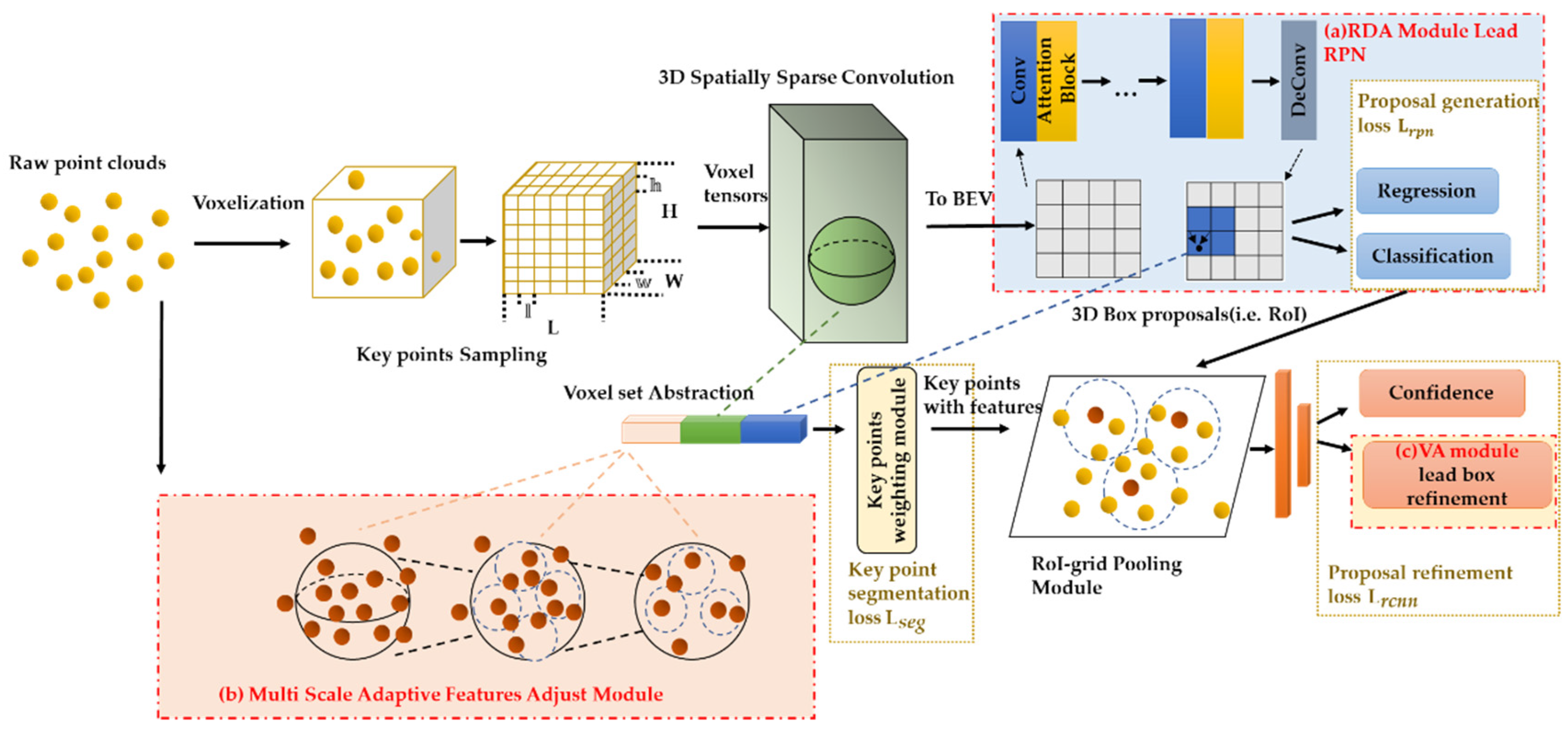
The overall architecture of our AFE-RCNN is shown in Figure 2. We propose three novel modules, i.e., (a) the residual of dual attention proposal generation module (RDA module) (Figure 2a); (b) multi-scale adaptive feature extraction module based on point clouds (MSAA) (Figure 2b); (c) refinement loss function module with vertex associativity (VA module) (
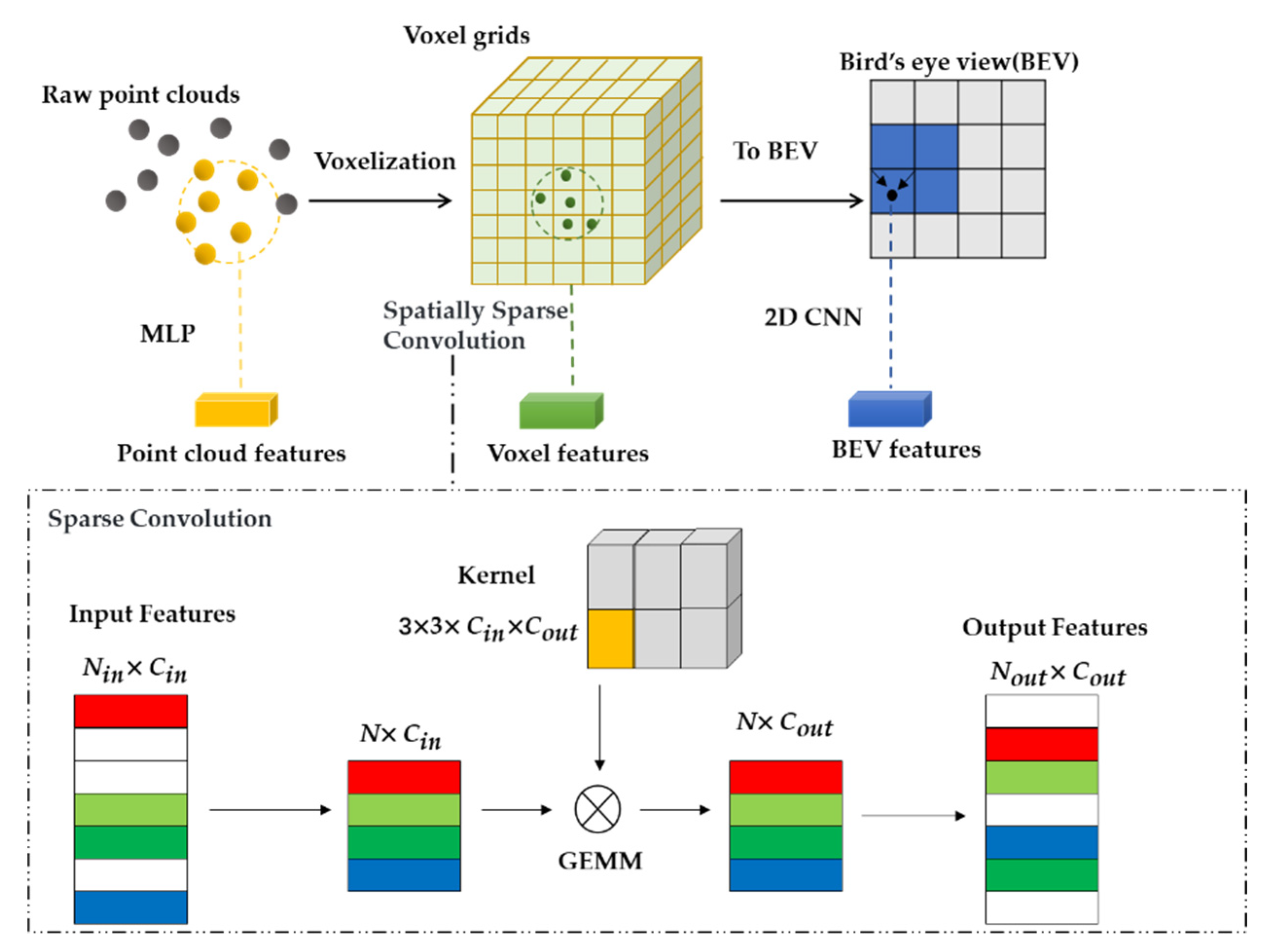
Figure 2c). In our AFE-RCNN, the input point clouds are processed by two branches; that is, a voxel-based branch and a point-based branch. In the voxel-based branch, we first voxelize the raw point clouds. Referring to ref. [17], we divide the raw point clouds into small voxel grids of the same scale in x,y,z directions. Then, we use the average of the features of all points inside the non-empty voxel as the features of the voxel. Secondly, we obtain the voxel features through a 3D spatially sparse convolutional network [10]. Next, we project the point clouds to the 2D BEV coordinate by eight times downsampling (i.e., stack the Z-axis features together to generate the 2D BEV feature maps), and obtain the 2D BEV features through the RDA module. Finally, the RPN generates box proposals based on the anchor box approach and BEV features. In the point-based branch, to summarize the information of the scene, we sample the key points through farthest point sampling (FPS), then the features of key points are obtained by MSAA. Next, as the rich features are beneficial to the box proposal refinement, the features of BEV, raw point clouds, and voxels are fused to build the key point features. To make the foreground points contribute more to refinement, the weights of the key points are adjusted by the weighting module (see ref. [17]). At last, the box proposal refinement is completed based on the key point features and the key point-to-grid RoI feature abstraction (see ref. [17]); the grid point is the center point of the voxel grid. We guarantee the correlation among the vertices of the box to optimize the box proposal regression by the advantages of the VA module. Details of the main operations are given in the subsections.

3.1. The Residual of Dual Attention Proposal Generation Module

Our AFE-RCNN firstly divides the raw point clouds into the several uniform scales of voxel grids, and then obtains the 3D voxel features through a 3D spatially sparse convolutional network. Secondly, the proposed network projects the information of 3D features to the 2D BEV coordinate. The network of the BEV feature extraction in ref. [17] consists of the traditional 2D CNN, which usually processes all features equivalently and cannot reflect the variability requirements in object detection tasks. Moreover, the extracted feature map only aggregates the spatial and channel information in the local receptive field, which will lead to a lack of relevance of global information.
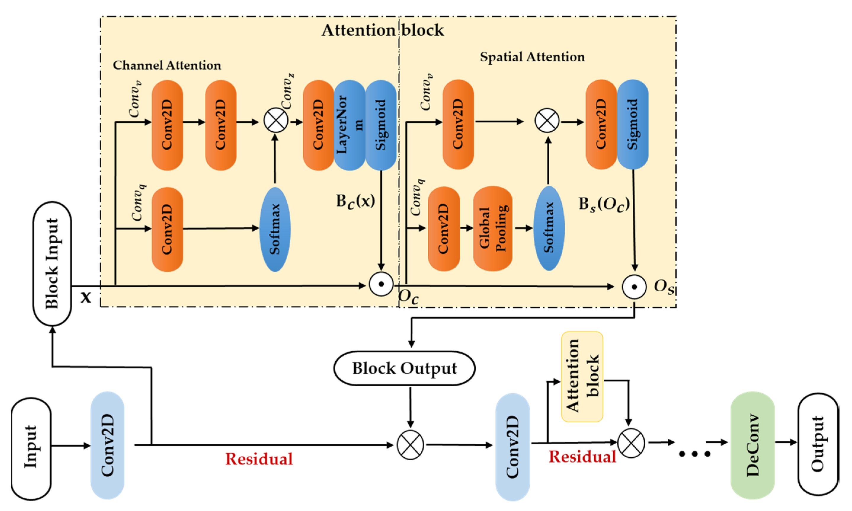
To solve the above problems, we propose the residual of dual attention proposal generation module (RDA module). Inspired by the polarized self-attention block [30], we construct the attention block by the residual connection to ensure the integrity of information transmission for feature processing, which can process both the spatial and channel dimensions of features with very little calculation increase. The diagram of the proposed RDA module is shown in Figure 3. The input of the module is used to mainly control the direction of information processing, avoiding the situation in which background points are overly focused. The proposed module can strengthen the correlation between object features in the spatial domain and global feature channel, which can fully excavate semantic information in both spatial dimension and channel dimension.
We first assume that the input features X are independent; the channel attention branch B c ( X ) R C × 1 × 1 is defined as Equation (1).
B c ( X ) = F S G [ C o n v z ( ( τ 1 ( C o n v v ( X ) ) × F S M ( τ 2 ( C o n v q ( X ) ) ) ]
where C n v q ,   C o n v v , and C o n v z are all 1 × 1 convolutional layers, τ 1 and τ 2 are two vector transformation symbols, × presents matrix dot product operation, F S G ( ) is a sigmoid operator, and F S M ( ) is a SoftMax operator. The output of channel attention branch is:
O c = B c ( X ) c X R C × H × W
where c is the channel multiplication operator.
Here, the spatial attention branch B s ( X ) R 1 × H × W is defined as Equation (3):
B s ( X ) = F S G [ τ 3 ( F S M ( τ 1 ( F G P ( C o n v q ( X ) ) ) ) × τ 2 ( C o n v v ( X ) ) ) ]
where τ 1 , τ 2 , and τ 3 are vector transformation symbols; F G P ( ) is a global pooling operator. The output of the spatial attention branch is shown as Equation (4). s is the spatial multiplication operator.
O s = B s ( O c ) s O c
The output of one residual block O r is:
O r = X +   ε O s
where ε is the weighting factor of the attention module. Here, the range of ε is 0~1; the best performance can be achieved when ε = 0 . 1 . After a lot of experiments, we found that the average running times before and after adding the RDA module to the RPN stage are ~0.0060 s and ~0.0071 s run on the same processor, respectively, which is a difference of milliseconds. The use of the attention network did not result in a significant decrease in the efficiency of our proposed network.

3.2. Multi-Scale Feature Extraction Module Based on Adaptive Feature Adjustment

In ref. [17], a certain number of points are sampled as the key points. That sampling approach may cause poor robustness features in the sparse region of the point clouds. To solve this problem, we propose a multi-scale feature extraction module based on adaptive feature adjustment (MSAA) as shown in Figure 4. Firstly, we sample 2048 points through FPS to summarize the information of the scene. This is followed by two times 4-fold downsampling and points grouping; the sampling layers with different scales that containing 512 and 128 points are obtained, respectively. Inspired by ref. [25], to extract richer feature information, we process the features for each grouping layer based on adaptive feature adjustment (AFA). The interaction between points can be found through the AFA, which can also integrate the neighboring contextual information into the features of each point. Moreover, the multi-scale point clouds can be constructed by different sampling and grouping layers. Thus, the features of all sampling layers are interpolated to the same feature shape and concatenated together, which can construct multi-scale features of the key points.
In the point cloud feature extraction for each sampling layer, first, the features of each point (Figure 4a) in the region Q consist of the feature set F , which can be expressed as F = { F 1 ,   F 2 ,…,   F n }. In order to focus on the correlation between each point pair, we connect the points in region Q into a local network, which can learn the interactions between all point pairs. We get the difference map F d i f ( i ) (Figure 4b) at the same time. And then, F d i f ( i ) learns the amount of impact among point features through the impact function to get the impact map β i  Figure 4c, this is so that the points in region Q can merge the neighboring contextual information, and the features of each point have better local neighborhood representation ability. The adjusted feature F i is defined as Equation (6).
F i = F i + F i m o d , F i m o d = f m o d u a l ( F i , F )
where F i is one of the features in the feature set F . F i m o d represents the amount of impact, which is affected by each feature in F on F i . F i m o d is obtained by adaptive learning of the feature modulator in the feature set F . The learning process of the feature modulator f m o d u a l is defined as Equation (7), where · means product operation.
f m o d u a l ( F i , F ) = j = 1 n f i m p a c t ( F i , F j )   f r e l a t i o n ( F i , F j )  
The learning process of the feature modulator is mainly involved in two functions; one is the amount of impact of F j on F i , which is represented by the function f i m p a c t . The other is the relation function f r e l a t i o n . The impact function f i m p a c t is calculated by the MLP operation. The function f i m p a c t is defined as Equation (8):
f i m p a c t ( F i , F j ) = MLP ( f r e l a t i o n ( F i , F j ) )
In the relation function f r e l a t i o n , the amount of impact is calculated by the difference between the two feature vectors F i and F j in feature set F . Specifically, when i = j , the amount of impact on F i is the feature F i itself. f r e l a t i o n is defined as Equation (9):
f r e l a t i o n ( F i , F j ) = { F i F j , i j F i , i = j  
For each feature in the local region Q, the total output of the learned feature is shown as Equation (10). Hence, F i incorporates contextual information from the entire region through the above densely connected local network of points.
F i =   β i ( i ) · F i + j = 1 , j i N β j ( i ) · ( F j   F i ) β j ( i ) = { f i m p a c t ( F i , F j ) ,   i j f i m p a c t ( F i , F j ) + 1 ,   i = j  
In different sampling layers, we firstly use interpolation to upsample the point clouds to the same number, and then concatenate these feature vectors as multi-scale features for key points. The interpolation process can be expressed as:
F j l a y ^ = j = 1 K ω j ( p i l a y ) F j l a y j = 1 K ω j ( p i l a y )
ω j ( p i ) = { 1 | | p i l a y p j l a y | | 2 , p j l a y P l a y ( p i l a y ) 0 ,   o t h e r
where p i l a y is one of the points in the sampling point set P l a y . F j l a y is the feature of p i l a y ; F j l a y ^ is the feature obtained by interpolation. We calculate the distance weight ω j between p i l a y and p j l a y through the K-nearest neighbors. As shown in Equation (12), the further away from p i l a y , the smaller the contribution on p i l a y . Here, K = 3.
In the point sampling and grouping stage, the feature set of the (k + 1)-th layer is ( k + 1 ) l a y , which is represented by Equation (10). To make the features of the (k + 1)-th layer consistent with the features of the previous layer in the point dimension, ( k + 1 ) l a y is processed by interpolation to obtain ( k + 1 ) l a y ^ . Finally, the previous layer F ( k ) l a y is obtained by concatenating ( k ) l a y and ( k + 1 ) l a y ^ . The feature set of the k-th layer is:
F ( k ) l a y = ( k + 1 ) l a y + ( k + 1 ) l a y ^ , k = 1 , 2 F ( k ) l a y = ( k ) l a y , k = 3
In addition, to provide rich feature information for box proposal refinement, we convert the BEV features obtained in Section 3.1 to key point features by bilinear interpolation, then the set abstraction operation in ref. [22] is used to fuse the features of voxels into key points. After the above operation, the features of BEV, raw point clouds, and voxels are fused as the key point features. Finally, we sample m grid points in each box proposal. Here, m = 216. For each grid point, we aggregate the features of neighboring key points to it to help the box proposal refinement.

3.3. Refinement Loss Function Module with Vertex Associativity

The refinement network is mainly used to learn the center point, size, and direction of the detection box. Two MLP layers are used to construct the refinement network, which finally performs the two tasks of confidence prediction and box regression. Generally, for the box regression loss, the vertices are usually regarded as independent of each other. However, the vertices of the bounding box are related to each other to a certain extent. The intersection over union (IoU) [33] is used to evaluate the effectiveness of the detection boxes. For different detection boxes, there may be a situation where the smooth-L1 loss is similar but the IoU varies greatly. In order to solve this problem, we propose the refinement loss function module with vertex associativity (VA module), as shown in Equation (14). The VA module trains the bounding box as a whole and solves the problem in which the anchor cannot be regressed when the prediction box does not intersect with the ground truth box.
L r e g ( x p r e ,   x g t ) = L s m o o t h _ L 1 ( x p r e ,   x g t ) + L c o r n e r + α L D I o U
The weight coefficient α of L D I o U is referred to the dataset and experiment. According to the statistics of multiple experiments, a better result can be achieved when the α value is in the range 0.1~1. The best performance can be achieved when α = 0.3. L s m o o t h _ L 1 and L c o r n e r are shown as Equations (15) and (16). c o r n p r e is the predicted corner; c o r n g t is the ground truth corner.
L s m o o t h _ L 1 ( x p r e ,   x g t ) = { 0.5 ( x p r e     x g t ) 2   i f   | x p r e x g t | < 1 | x p r e     x g t |     0.5 o t h e r w i s e
L c o r n e r = m e a n ( L s m o o t h _ L 1 ( c o r n p r e , c o r n g t ) )
Here, the normalized distance between the center points of the prediction box and the ground truth box is directly minimized to achieve rapid convergence. We choose the height value of the 3D bounding box within a certain angular range on the lidar coordinate. The height values are then normalized as a partial value for the length and width of the bounding box. We project the 3D bounding box to the 2D BEV coordinate through the above approach, so that the DIoU can be calculated by the 2D BEV information. LDIoU is shown as Equation (17) [35]:
L D I o U = L I o U + ρ 2 ( b , b g t ) c 2
where b represents the center point of the prediction box; b g t is the center point of the ground truth box. ρ ( ) represents the function of the Euclidean distance between two center points. c represents the diagonal distance of the smallest rectangle that can cover the predicted box and the ground truth box at the same time.
For the confidence prediction, the IoU between the ground truth boxes and the box proposals are used as the optimization object.
L I o U = u k log ( u k ˜ )     ( 1     u k )   log ( 1   u k ˜ )
Here, u k is the confidence of the optimization object for the k-th box proposals. u k ˜ is the predicted score.

3.4. Training Losses

Our AFE-RCNN is trained end-to-end. According to Figure 2, the training losses L t r a i n consist of the region proposal loss L r p n , the segmentation loss L s e g , and the refinement loss L r c n n .
1
The proposal generation network performs the classification and regression of anchor boxes based on the BEV features. The region proposal loss L r p n is:
L r p n = L c l s + L s m o o t h _ L 1 ( ϑ ˜ g e n , ϑ g e n )
Among them, the anchor box regression is calculated through L s m o o t h _ L 1 . ϑ ˜ g e n is the predicted residual for the anchor box; ϑ g e n is the regression target for the anchor box. ϑ ˜ g e n ,   ϑ g e n represents the position parameters (x, y, z, h, l, w) and pose parameters ( θ ) of the 3D bounding box. L c l s is the anchor classification loss as shown in Equation (20).
L c l s = { β ( 1 X ~ ) g log ( X ~ ) ,   X = 1 ( 1 β ) X ~ g log ( 1 X ~ ) ,   X = 0
Among them, X   { 0 , 1 } is the ground truth label; X ~ is the predicted input. β is the balance factor; g is the focusing parameter that is used to adjust the sample weights. Here, we set β = 0.25, g = 2.0.
2
The key point segmentation loss L s e g   is used to filter the foreground, where the calculation method is the same as the classification loss L c l s .
3
The refinement network performs the confidence prediction and regression of the box proposals based on the rich feature information of key points. L I o U is used for confidence prediction, while L r e g in Section 3.3 is used for box regression. The proposal refinement loss L r c n n is:
L r c n n = L I o U + L r e g ( ϑ ~ r e f , ϑ r e f )
Among them, ϑ ~ r e f is the predicted box residual; ϑ r e f is the proposal regression object. ϑ ~ r e f , ϑ r e f represent the position parameters and pose parameters of the bounding box.
The training loss L t r a i n   can now be expressed as the Equation (22):
L t r a i n = L r p n + L s e g   +   L r c n n

4. Experiments and Results

In the experimental part, we first test AFE-RCNN on the KITTI dataset and compare it with the state-of-art methods, then we conduct ablation experiments to verify the effectiveness of each part for the proposed AFE-RCNN. In addition, we also conduct experiments on the Waymo dataset to prove the robustness of AFE-RCNN.

4.1. Dataset and Implementation Details

KITTI dataset: The KITTI dataset is widely used in the evaluation of 3D object detection networks. The annotation file of KITTI contains 15 items, which indicate target category, truncation rate, occlusion level, observation angle (−π~π), 2D bounding box coordinates, height, width, and length of the 3D bounding box, 3D coordinates of the object position in camera coordinates, and the rotation angle relative to the y axis. The detection task is divided into three difficulty levels, i.e., easy, moderate, and hard. The objects in the easy level are fully visible, while their minimum bounding box height is 40 pixels and maximum cutoff is 15%. The objects in the moderate level are partially occluded, while their minimum bounding box height is 25 pixels and maximum cutoff is 30%. The objects in the hard level are difficult to observe, while their minimum bounding box height is 25 pixels and maximum cutoff is 50%. We compared AFE-RCNN with the state-of-the-art methods on the online test server, and conducted ablation experiments on the validation set. For voxelization, we set the point cloud range as (0, 70.4) m in the X axis, (−40, 40) m in the Y axis, and (−3, 1) m in the Z axis. We also set the size of voxel grids as (0.05, 0.05, 0.1) m.
The training and test sets contain 7481 training samples and 7518 test samples, respectively. In the evaluation of the test set, we randomly divided 80% of the training set for training and the remaining 20% for validation. In the ablation experiment, we randomly divided the training data into 3712 training split and 3769 validation split.
According to ref. [36] and the KITTI official metrics, we set the IoU threshold for the car class as 0.7 and for the cyclist class as 0.5. The mAP | 40 and the average orientation similarity ( AOS | 40 ) calculated from 40 recall positions were used as the evaluation indicators for the test sets and the validation sets. The mAP was calculated on the set of recall R n = { 1 / n , 2 / n , , 1 } as Equation (23):
mAP | R = 1 | R | r R ρ i n t e r p ( r )
where Θ o b j represents the target box, Θ d e t represents the detected box, ρ i n t e r p ( r ) = max r : r r ρ ( r ) . ρ ( r ) represents the precision calculated at the recall position r .
The AOS is calculated as Equation (24):
AOS = 1 | R | r R max r : r r s ( r )
where s ( r ) represents the orientation similarity rate calculated at the recall position r .
Waymo open dataset: The Waymo dataset is a large-scale 3D detection dataset. The training set has 798 sequences while the validation set has 202 sequences. The objects in the Waymo dataset are divided into two difficulty levels; level one comprises objects containing at least five points, and level two comprises objects containing at least one point or objects directly marked as level two. For voxelization, we set the point cloud range as (−75.2, 75.2) m for the X and the Y axes, and (−2, 4) m for the Z axis. We set the size of voxel grids as (0.1, 0.1, 0.15) m.
We used 200 sequences for training and in total 202 sequences for validation. The mAP and the mean average precision weighted by heading (mAPH) [2] are two official evaluation indicators, which were used to evaluate the performance of our AFE-RCNN in vehicle (IoU thresh = 0.7) and cyclist (IoU thresh = 0.5) detection.
Implementation details: Our AFE-RCNN is optimized by the ADAM optimizer. On the KITTI dataset, we trained our network with the batch size 6 and initial learning rate 0.01 for 80 epochs on 3 RTX 2080 GPUs. On the Waymo dataset, we trained our network with the batch size 4 and initial learning rate 0.01 for 30 epochs on 2 RTX 2080 GPUs.

4.2. Evaluation on the KITTI Online Test Server

We evaluated the test set based on the KITTI official test server and compared the performance of AFE-RCNN with the state-of-the-art methods. The results are shown in Table 2 and Table 3.
According to the official information from the KITTI benchmark, we mainly compared the performance of AFE-RCNN with the state-of-the-art methods on moderate-difficulty mAP | 40 as of 5 January 2022. The following conclusions can be observed from Table 2 and Table 3 and Figure 5. Note that refs. [9,37] do not list the performance of orientation. These papers are not focused on the 3D object orientation evaluation, which mainly provides the mAP | 40 of cars. To ensure the fairness of the comparisons, the comparison algorithms used in Table 2 and Table 3 are different according to the results provided in the corresponding references.
For the performance of 3D detection, our AFE-RCNN has 3 evaluation indicators (total 6 indicators) ranked Top 1 of all comparison algorithms as shown in Table 2. Besides, from the results shown in Table 2, we can make the following observations.
(1) Our AFE-RCNN outperforms the voxel-based methods on moderate and hard difficulty levels of the car and all difficulty levels of the cyclist. For cars, our network improves at least 1.25% on the moderate-difficulty mAP | 40 than the compared voxel-based methods. For cyclists, our network improves at least 3.98% on the moderate-difficulty mAP | 40 than the compared voxel-based methods. (2) Our AFE-RCNN outperforms the point-based methods on moderate and hard difficulty levels of cars and all difficulty levels of cyclists. For cars, our network improves at least 1.41% on the moderate-difficulty mAP | 40 than the compared point-based methods. For cyclists, our network improves at least 3.40% on the moderate-difficulty mAP | 40 than the compared point-based methods. (3) Compared with the method combining point clouds and voxels, our AFE-RCNN reaches 81.53% on the moderate-difficulty level mAP | 40 for cars, which is comparable to the 81.55% of mAP | 40 in ref. [38]. In all the difficulty levels for cyclists, our AFE-RCNN outperforms the compared algorithms.
For the performance of orientation estimation, our AFE-RCNN has 5 evaluation indicators ranked Top 3 of all comparison algorithms. As shown in Table 3, 3 indicators of our AFE-RCNN ranked first, and 2 indicators of our AFE-RCNN ranked second. From the results listed in Table 3, it is easily to draw the conclusions below.
(1) Our AFE-RCNN outperforms the voxel-based methods in 5 evaluation indicators. For cars, our network improves at least 0.86% on the moderate-difficulty AOS | 40 than the compared voxel-based methods. For cyclists, our network improves at least 1.66% on the moderate-difficulty AOS | 40 than the compared voxel-based methods. (2) Our AFE-RCNN outperforms the point-based methods in 5 evaluation indicators. For cars, our network improves at least 0.41% on the moderate-difficulty AOS | 40 than the compared point-based methods. For cyclists, our network improves at least 6.37% on the moderate-difficulty AOS | 40 than the compared point-based methods. (3) Compared with the method combining point clouds and voxels, our AFE-RCNN outperforms the compared algorithms in 3 evaluation indicators. For cars, our network improves at least 0.22% on the hard-difficulty AOS | 40 than the compared combining methods. For cyclists, our network improves at least 2.46% on the easy-difficulty AOS | 40 than the compared combining methods.

4.3. Ablation Experiments Based on KITTI Validation Set

To evaluate the individual components of our method, we conducted ablation experiments. As AFE-RCNN is proposed based on PV-RCNN, we regarded PV-RCNN as the baseline from which to compare the performance of each module. The ablation experiment results are shown in Table 4. Note that we used the same metric as the ablation experiment in PV-RCNN, i.e., the mAP | 40 was calculated with 40 recall positions. The experiments show that each component of AFE-RCNN has a performance gain on the original model.
Effect of RDA module: The RDA module learns the relevance of features in both channel and spatial dimensions, and assigns weights to features to suppress background points by filtering high-value features. This module improves the precision of subsequent processing. As shown in Table 4, Ours1 outperforms PV-RCNN with 0.08%, 0.46%, and 0.12% of mAP | 40 gains at each difficulty level for cars. For cyclists, Ours1 can also outperform PV-RCNN with 1.49%, 1.77%, and 1.52% of mAP | 40 gains at each difficulty level, which proves that the RDA module can achieve obvious improvements.
Effect of MSAA: We performed three levels of feature extraction on the raw point clouds. The MSAA ensures the robustness of sampling in sparse regions of the point cloud by multi-scale grouping and sampling and finds the interaction between points in a local region base on the adaptive feature adjustment method. According to Table 4, Ours2 outperforms Ours1 with 0.09%, 0.23%, and 0.31% of mAP | 40 gains at each difficulty level for cars, and Ours2 can also outperform Ours1 with 0.62%, 2.86%, and 2.67% of mAP | 40 gains at each difficulty level for cyclists. Besides, compared with PV-RCNN, the 3D detection mAP | 40 of Ours2 at each difficulty level of the car has improved by 0.17%, 0.69%, and 0.43%, respectively. At the same time, the 3D detection mAP | 40 of Ours2 at each difficulty level of the cyclist has improved by 2.11%, 4.63%, and 4.19%, respectively. We note that the gain brought by the MSAA module is the most obvious, especially for cyclists. The possible reasons can be summarized in the following two aspects. Firstly, directly processing the raw point clouds can effectively reduce the information loss. Secondly, benefiting from the multi-scale network structure and the method of adaptive feature adjustment, the points in the local region can better aggregate the regional contextual information.
Effect of VA module: To avoid the problem in which the correlation among the vertices of the bounding box is ignored, we optimized the loss function based on DIoU Loss. Experiments show that the AFE-RCNN has a certain improvement when compared with Ours2; the 3D detection mAP | 40 of AFE-RCNN at each difficulty level of the car has improved by 0.08%, 0.26%, and 0.17%, respectively. At the same time, the 3D detection mAP | 40 of AFE-RCNN at each difficulty level of the cyclist has improved by 0.33%, 0.38%, and 0.43%.
Compared with PV-RCNN: According to Table 4, our AFE-RCNN has 10 evaluation indicators (total 12 indicators) better than the PV-RCNN. For the 3D detection mAP | 40 , AFE-RCNN outperforms PV-RCNN with 0.25%, 0.95%, and 0.60% of mAP | 40 gains at each difficulty level for cars, and AFE-RCNN has improved by 2.44%, 5.01%, and 4.62% for cyclists than PV-RCNN. For the orientation estimation, AFE-RCNN outperforms PV-RCNN with 0.03% and 1.94% of AOS | 40 gains at moderate and hard difficulty levels for cars, and outperforms PV-RCNN with 2.13% and 3.13% of AOS | 40 gains at moderate and hard difficulty levels for cyclists.
In addition, we conducted experiments to analyze the attention mechanisms. As shown in Table 5, we found that the performance of our method becomes worse after directly adding the dual attention block (DA block). For cyclists in the moderate level, the mAP | 40 of baseline with the DA block is decreased by 0.27% compared to the baseline. However, when we used the residual module to connect the dual attention block (RDA block), the baseline with RDA block has 1.77% mAP | 40 gains for the moderate level of cyclists. Compared to adding the DA block directly, the performance of adding the RDA block can be significantly improved, which can prove the residual connection is effective for the attention module.
From the results in Table 2, Table 3 and Table 4, we observe that the performance for cyclists has a significant improvement. As these objects are small and may have fewer sampling points, the limited number of points makes it hard to provide sufficient semantic information. We fully excavated the relevance and contextual semantic information among the key points to make the feature information in the cyclist class more representative. However, there is little improvement for the performance of the easy difficulty level, which means that our method has a limited effect with enough object points.

4.4. Evaluation on the KITTI Validation Set

For most related papers that have conducted experiments on the KITTI validation set, they only provide the mAP | 11 (calculated with 11 recall positions) of 3D detection for cars. We followed this metric [45] and compare our AFE-RCNN with the state-of-the-art methods in Table 6.
Our AFE-RCNN has 2 evaluation indicators (total 3 indicators) ranked Top 3 for all comparison algorithms. Considering the number of indicators ranked Top 3, our method has a certain advantage. Our method does not outperform in all indicators, which may be related to the different divisions of the training and validation sets. When compared with the baseline method, our AFE-RCNN outperforms the PV-RCNN at all difficulty levels. The 3D detection mAP | 11 has improved by 0.27%, 0.30%, and 0.48%, respectively.

4.5. Qualitative Analysis on the KITTI Dataset

We compared the visualization results of AFE-RCNN with PV-RCNN. To further demonstrate the advantages of our method, we compared PointRCNN [7] as well. As shown in Figure 6, the red boxes represent the prediction boxes, while the green and yellow represent the ground truth boxes for car and cyclist, respectively. It can be seen that PointRCNN has missing detection in the cyclist class, whereas the PV-RCNN and our AFE-RCNN have more comprehensive detection. This is because the method of PointRCNN obtains less feature information and lacks correlation as it simply processes the raw point clouds only. Our AFE-RCNN uses the feature enhancement method to extract the features of the raw point clouds and BEV. These two features are then fused with voxel features for key point features. The rich feature information leads to a better detection performance. Furthermore, the prediction boxes of AFE-RCNN are closer to the ground truth than PV-RCNN and PointRCNN.

4.6. Validation on the Waymo Open Dataset

We used our AFE-RCNN on the Waymo dataset to illustrate the effectiveness of AFE-RCNN, and the results are shown in Table 7. We validated two classes of objects, i.e., vehicle and cyclist, and compared the results of two official evaluation indicators, i.e., mAP and mAPH [2]. According to Table 7, we can make the following conclusions.
Comparison with the state-of-the-art methods. For the vehicle, our AFE-RCNN has a relatively outstanding performance. The AFE-RCNN outperforms the compared algorithms with at least 5.14% and 4.52% mAPH gains on two 3D object detection difficulty levels. For the cyclist, the performance of our AFE-RCNN is worse than Centerpoint [47]. However, the performance of AFE-RCNN is obviously better than the other compared methods. Since our AFE-RCNN uses the anchor-based method to generate the detection boxes, when the object is tilted to a certain angle, the anchor-based method cannot coordinate this angle well, which results in a large error. The Centerpoint [47] uses a center-based method that takes advantage of the rotational invariance of the point clouds to solve this problem.
Compared with PV-RCNN. For the vehicle, the performance of our AFE-RCNN has small improvements over the PV-RCNN. However, for the cyclist, our AFE-RCNN outperforms the compared algorithms with 2.85% and 2.40% mAPH gains on two 3D object detection difficulty levels. This proves that our proposed method for the improvement of PV-RCNN is effective.

4.7. Efficiency and Robustness Analysis of the Proposed Algorithm

To verify the efficiency of the proposed algorithm, the running times of our algorithm on the validation sets of the KITTI and Waymo open datasets are shown in Table 8. Compared to the baseline, the running time of our algorithm has a millisecond increase. However, according to the Table 2, Table 7 and Table 8, the proposed AFE-RCNN can obtain better detection accuracy with a small increase in time, which can achieve promising performance in both accuracy and efficiency for the 3D object detection task.
To analyze the class number of the objects’ impact on the efficiency and precision of our algorithm, we conducted experiments for multiple objects on the validation set of KITTI. The results are shown in Table 9. Taking the car category as an example, the mAP | 40 values in three groups of experiments are 85.33%, 85.29%, and 85.31%. The class number of the objects has a very small impact on the performance ( mAP | 40 ) of our AFE-RCNN. Meanwhile, the running time of our AFE-RCNN for different class numbers of object detection has only a slight effect (<0.001 s). The results demonstrate that our algorithm maintains a good efficiency and robustness when performing multiple object detection.
In addition, to further verify the robustness of the proposed algorithm, we conducted the experiments for pedestrian detection on the validation set of KITTI. As shown in Table 10, our AFE-RCNN outperforms the baseline on all the difficulty levels. Taking the performance on the moderate difficulty level as an example, our AFE-RCNN outperforms the baseline with 5.18% mAP | 40 gains and 4.11% AOS | 40 gains. The results prove that our AFE-RCNN is robust and can achieve good performance in small object detection.

5. Conclusions

We have proposed a 3D object detection method known as AFE-RCNN. Firstly, to generate high-quality proposal frames, we focused on the relationship between features in both channel dimension and spatial dimension through the RDA module. Secondly, we used multi-scale sampling and adaptive methods to robustly obtain fine local information on key points. Finally, based on the rich feature information on the key points, we completed the proposal refinement through the VA module, which guarantees correlation among the vertices of the box proposals. When compared with the state-of-the-art methods, AFE-RCNN can achieve a comparable performance; especially the cyclist class with a relatively small size has a significant improvement. However, to satisfy the requirements of time-sensitivity in object detection tasks, we need to study a lightweight method that can improve the detection precision while also ensuring computational efficiency. In the future, we will try to combine point clouds with 2D image information and replace the excessive detail processing of point clouds by a lightweight image feature extraction method. The gain from lightweight image processing to replace the much-detailed processing of point clouds only is a potential research direction.

Author Contributions

H.H., Y.L. and F.S. developed the AFE-ECNN algorithm. Y.L. assisted in the development of a complete set of 3D object detection algorithms. H.H. and R.Q. completed the visualization of results and wrote the source code and the manuscript. F.S. and H.H. helped with the data analysis and experimental analysis. P.L. and Y.L. helped with the paper writing and analysis of the results. All authors have read and agreed to the published version of the manuscript.

Funding

This work was supported by the Guangxi Key Laboratory of Manufacturing System & Advanced Manufacturing Technology (Grant No.20-065-40S005), the Key Laboratory of Advanced Manufacturing technology, Ministry of Education (Grant No. GZUAMT2021KF04), and the National Natural Science Foundation of China (Grant No. 61720106009). The authors gratefully acknowledge language help from the other members in the Guangxi Key Laboratory of Manufacturing System & Advanced Manufacturing Technology. And the APC was funded by F.S. and Y.L.

Data Availability Statement

The data presented in this study are openly available in [1,2].

Acknowledgments

The authors thanks Jianchuan Qin, Xiuning Liu and Qipeng Pu for helping with the draft writing and checking.

Conflicts of Interest

The authors declare no conflict of interest.

References

  1. Geiger, A.; Lenz, P.; Stiller, C.; Urtasun, R. Vision meets robotics: The KITTI dataset. Int. J. Robot. Res. 2013, 32, 1231–1237. [Google Scholar] [CrossRef] [Green Version]
  2. Sun, P.; Kretzschmar, H.; Dotiwalla, X.; Chouard, A.; Patnaik, V.; Tsui, P.; Guo, J.; Zhou, Y.; Chai, Y.; Caine, B.; et al. Scalability in Perception for Autonomous Driving: Waymo Open Dataset. In Proceedings of the IEEE Conference on Computer Vision and Pattern Recognition (CVPR), Seattle, WA, USA, 13–19 June 2020; pp. 2443–2451. [Google Scholar]
  3. Hornik, K. Approximation capabilities of multilayer feedforward networks. Neural Netw. 1991, 4, 251–257. [Google Scholar] [CrossRef]
  4. Wang, Q.; Chen, J.; Deng, J.; Zhang, X. 3D-CenterNet: 3D object detection network for point clouds with center estimation pri-ority. Pattern Recognit. 2021, 115, 107884. [Google Scholar] [CrossRef]
  5. Wang, L.; Zhao, D.; Wu, T.; Fu, H.; Wang, Z.; Xiao, L.; Xu, X.; Dai, B. Drosophila-inspired 3D moving object detection based on point clouds. Inf. Sci. 2020, 534, 154–171. [Google Scholar] [CrossRef]
  6. Li, X.; Guivant, J.; Khan, S. Real-time 3D object proposal generation and classification using limited processing resources. Robot. Auton. Syst. 2020, 130, 103557. [Google Scholar] [CrossRef]
  7. Shi, S.; Wang, X.; Li, H. Pointrcnn: 3d Object Proposal Generation and Detection From Point Cloud. In Proceedings of the IEEE Conference on Computer Vision and Pattern Recognition, Long Beach, CA, USA, 15–20 June 2019; pp. 770–779. [Google Scholar]
  8. Shi, W.; Rajkumar, R. Point-GNN: Graph Neural Network for 3D Object Detection in a Point Cloud. In Proceedings of the 2020 IEEE/CVF Conference on Computer Vision and Pattern Recognition (CVPR), Seattle, WA, USA, 13–19 June 2020; pp. 1708–1716. [Google Scholar]
  9. Yang, Z.; Sun, Y.; Liu, S.; Jia, J. 3DSSD: Point-Based 3D Single Stage Object Detector. In Proceedings of the 2020 IEEE/CVF Conference on Computer Vision and Pattern Recognition (CVPR), Seattle, WA, USA, 13–19 June 2020; pp. 11037–11045. [Google Scholar]
  10. Yan, Y.; Mao, Y.X.; Li, B. SECOND: Sparsely Embedded Convolutional Detection. Sensors 2018, 18, 3337. [Google Scholar] [CrossRef] [PubMed] [Green Version]
  11. Shi, S.; Wang, Z.; Shi, J.; Wang, X.; Li, H. From Points to Parts: 3D Object Detection from Point Cloud with Part-aware and Part-aggregation Network. IEEE Trans. Pattern Anal. Mach. Intell. 2020, 43, 2647–2664. [Google Scholar] [CrossRef] [PubMed] [Green Version]
  12. Ye, Y.; Chen, H.; Zhang, C.; Hao, X.; Zhang, Z. Sarpnet: Shape attention regional proposal network for lidar-based 3d object detection. Neurocomputing 2020, 379, 53–63. [Google Scholar] [CrossRef]
  13. Wang, L.; Fan, X.; Chen, J.; Cheng, J.; Tan, J.; Ma, X. 3D object detection based on sparse convolution neural network and feature fusion for autonomous driving in smart cities. Sustain. Cities Soc. 2020, 54, 102002. [Google Scholar] [CrossRef]
  14. Zheng, W.; Tang, W.; Chen, S.; Jiang, L.; Fu, C.W. CIA-SSD: Confident IoU-Aware Single-Stage Object Detector from Point Cloud. arXiv 2020, arXiv:2012.03015. [Google Scholar]
  15. Lang, A.H.; Vora, S.; Caesar, H.; Zhou, L.; Yang, J.; Beijbom, O. PointPillars: Fast Encoders for Object Detection from Point Clouds. In Proceedings of the 2019 IEEE/CVF Conference on Computer Vision and Pattern Recognition (CVPR), Long Beach, CA, USA, 18–20 June 2019; pp. 12697–12705. [Google Scholar]
  16. Du, L.; Ye, X.; Tan, X.; Feng, J.; Xu, Z.; Ding, E.; Wen, S. Associate-3Ddet: Perceptual-to-conceptual association for 3D point cloud object detection. In Proceedings of the 2020 IEEE/CVF Conference on Computer Vision and Pattern Recognition (CVPR), Seattle, WA, USA, 13–19 June 2020; pp. 13326–13335. [Google Scholar]
  17. Shi, S.; Guo, C.; Jiang, L.; Wang, Z.; Shi, J.; Wang, X.; Li, H. PV-RCNN: Point-Voxel Feature Set Abstraction for 3D Object Detection. In Proceedings of the 2020 IEEE/CVF Conference on Computer Vision and Pattern Recognition (CVPR), Seattle, WA, USA, 13–19 June 2020; pp. 10526–10535. [Google Scholar]
  18. Graham, B.; Maaten, L. Submanifold sparse convolutional networks. arXiv 2017, arXiv:1706.01307. [Google Scholar]
  19. Yang, B.; Liang, M.; Urtasun, R. Hdnet: Exploiting hd maps for 3d object detection. Conference on Robot Learning. PMLR 2018, 87, 146–155. [Google Scholar]
  20. Chen, X.; Ma, H.; Wan, J.; Li, B.; Xia, T. Multi-view 3D Object Detection Network for Autonomous Driving. In Proceedings of the IEEE Conference on Computer Vision and Pattern Recognition, Honolulu, HI, USA, 21–26 July 2017; pp. 1907–1915. [Google Scholar]
  21. Qi, C.R.; Su, H.; Mo, K.; Guibas, L.J. Pointnet: Deep learning on point sets for 3d classification and segmentation. In Proceedings of the IEEE Conference on Computer Vision and Pattern Recognition, Honolulu, HI, USA, 21–26 July 2017; pp. 652–660. [Google Scholar]
  22. Charles, R.Q.; Li, Y.; Hao, S.; Guibas, L.J. Pointnet++: Deep hierarchical feature learning on point sets in a metric space. Adv. Neural Inf. Process. Syst. 2017, 30, 5099–5108. [Google Scholar]
  23. Wang, Y.; Sun, Y.; Liu, Z.; Sarma, S.E.; Bronstein, M.M.; Solomon, J. Dynamic Graph CNN for Learning on Point Clouds. ACM Trans. Graph. 2019, 38, 1–12. [Google Scholar] [CrossRef] [Green Version]
  24. Li, Y.; Bu, R.; Sun, M.; Wu, W.; Di, X.; Chen, B. Pointcnn: Convolution on x-transformed points. Adv. Neural Inf. Process. Syst. 2018, 31, 820–830. [Google Scholar]
  25. Zhao, H.; Jiang, L.; Fu, C.-W.; Jia, J. PointWeb: Enhancing Local Neighborhood Features for Point Cloud Processing. In Proceedings of the 2019 IEEE/CVF Conference on Computer Vision and Pattern Recognition (CVPR), Long Beach, CA, USA, 18–20 June 2019; pp. 5560–5568. [Google Scholar]
  26. Hu, J.; Shen, L.; Sun, G. Squeeze-and-Excitation Networks. In Proceedings of the IEEE Conference on Computer Vision and Pattern Recognition, Salt Lake City, UT, USA, 18–23 June 2018; pp. 7132–7141. [Google Scholar]
  27. Woo, S.; Park, J.; Lee, J.; Kweon, I.S. CBAM: Convolutional Block Attention Module. In Proceedings of the European Conference on Computer Vision, Munich, Germany, 8–14 September 2018. [Google Scholar]
  28. Wang, F.; Jiang, M.; Qian, C.; Yang, S.; Li, C.; Zhang, H.; Wang, X.; Tang, X. Residual Attention Network for Image Classification. In Proceedings of the IEEE Conference on Computer Vision and Pattern Recognition, Honolulu, HI, USA, 21–26 July 2017; pp. 3156–3164. [Google Scholar]
  29. Fu, J.; Liu, J.; Tian, H.; Li, Y.; Bao, Y.; Fang, Z.; Lu, H. Dual Attention Network for Scene Segmentation. In Proceedings of the 2019 IEEE/CVF Conference on Computer Vision and Pattern Recognition (CVPR), Long Beach, CA, USA, 15–20 June 2019; pp. 3146–3154. [Google Scholar]
  30. Liu, H.; Liu, F.; Fan, X.; Huang, D. Polarized Self-Attention: Towards High-quality Pixel-wise Regression. arXiv 2021, arXiv:2107.00782. [Google Scholar]
  31. Zhang, Y.; Li, K.; Li, K.; Wang, L.; Zhong, B.; Fu, Y. Image super-resolution using very deep residual channel attention networks. In Proceedings of the European Conference on Computer Vision, Munich, Germany, 8–14 September 2018; pp. 286–301. [Google Scholar]
  32. Girshick, R. Fast R-CNN. In Proceedings of the IEEE International Conference on Computer Vision, Santiago, Chile, 13–16 December 2015; pp. 1440–1448. [Google Scholar]
  33. Yu, J.; Jiang, Y.; Wang, Z.; Cao, Z.; Huang, T. Unitbox: An advanced object detection network. In Proceedings of the 24th ACM international conference on Multimedia, New York, NY, USA, 15–19 October 2016; pp. 516–520. [Google Scholar]
  34. Rezatofighi, H.; Tsoi, N.; Gwak, J.; Sadeghian, A.; Reid, I.; Savarese, S. Generalized Intersection Over union: A metric and a Loss for Bounding Box Regression. In Proceedings of the IEEE Conference on Computer Vision and Pattern Recognition, Long Beach, CA, USA, 18–20 June 2019; pp. 658–666. [Google Scholar]
  35. Zheng, Z.; Wang, P.; Liu, W.; Li, J.; Ye, R.; Ren, D. Distance-IoU loss: Faster and better learning for bounding box regression. In Proceedings of the AAAI Conference on Artificial Intelligence, New York, NY, USA, 7–12 February 2020; Volume 34, pp. 12993–13000. [Google Scholar]
  36. Simonelli, A.; Bulo, S.R.; Porzi, L.; Lopez-Antequera, M.; Kontschieder, P. Disentangling Monocular 3D Object Detection. In Proceedings of the 2019 IEEE/CVF International Conference on Computer Vision (ICCV), Seoul, Korea, 27 October 2019; pp. 1991–1999. [Google Scholar]
  37. Zhang, H.; Yang, D.; Yurtsever, E.; Redmill, K.A.; Ozguner, O. Faraway-Frustum: Dealing with Lidar Sparsity for 3D Object Detection using Fusion. In Proceedings of the IEEE International Intelligent Transportation Systems Conference, Indianapolis, IN, USA, 19–22 September 2021; pp. 2646–2652. [Google Scholar]
  38. Deng, J.; Zhou, W.; Zhang, Y.; Li, H. From Multi-View to Hollow-3D: Hallucinated Hollow-3D R-CNN for 3D Object Detection. IEEE Trans. Circuits Syst. Video Technol. 2021, 31, 4722–4734. [Google Scholar] [CrossRef]
  39. Gustafsson, F.K.; Danelljan, M.; Schon, T.B. Accurate 3D Object Detection using Energy-Based Models. In Proceedings of the IEEE Conference on Computer Vision and Pattern Recognition, Nashville, TN, USA, 19–25 June 2021; pp. 2855–2864. [Google Scholar]
  40. Huang, T.; Liu, Z.; Chen, X.; Bai, X. EPNet: Enhancing Point Features with Image Semantics for 3D Object Detection. In Proceedings of the European Conference on Computer Vision, Glasgow, UK, 23–28 August 2020; pp. 35–52. [Google Scholar]
  41. Li, J.; Dai, H.; Shao, L.; Ding, Y. Anchor-free 3D Single Stage Detector with Mask-Guided Attention for Point Cloud. In Proceedings of the 29th ACM International Conference on Multimedia, Chengdu, China, 20–24 October 2021; pp. 553–562. [Google Scholar]
  42. Liu, Z.; Zhao, X.; Huang, T.; Hu, R.; Zhou, Y.; Bai, X. TANet: Robust 3D Object Detection from Point Clouds with Triple Attention. In Proceedings of the AAAI Conference on Artificial Intelligence, New York, NY, USA, 7–12 February 2020; Volume 34, pp. 11677–11684. [Google Scholar]
  43. He, C.; Zeng, H.; Huang, J.; Hua, X.-S.; Zhang, L. Structure Aware Single-Stage 3D Object Detection from Point Cloud. In Proceedings of the 2020 IEEE/CVF Conference on Computer Vision and Pattern Recognition (CVPR), Seattle, WA, USA, 13–19 June 2020; pp. 11873–11882. [Google Scholar]
  44. Xu, Q.; Zhou, Y.; Wang, W.; Qi, C.R. Spg: Unsupervised domain adaptation for 3d object detection via semantic point generation. In Proceedings of the IEEE International Conference on Computer Vision, Virtual. 21–25 June 2021; pp. 15446–15456. [Google Scholar]
  45. He, Y.; Xia, G.; Luo, Y.; Su, L.; Zhang, Z.; Li, W.; Wang, P. DVFENet: Dual-branch voxel feature extraction network for 3D object detection. Neurocomputing 2021, 459, 201–211. [Google Scholar] [CrossRef]
  46. Zheng, W.; Tang, W.; Jiang, L.; Fu, C.-W. SE-SSD: Self-Ensembling Single-Stage Object Detector from Point Cloud. In Proceedings of the 2021 IEEE/CVF Conference on Computer Vision and Pattern Recognition, Nashville, TN, USA, 20–25 June 2021; pp. 14494–14503. [Google Scholar]
  47. Yin, T.; Zhou, X.; Krahenbuhl, P. Center-based 3D Object Detection and Tracking. In Proceedings of the IEEE Conference on Computer Vision and Pattern Recognition, Nashville, TN, USA, 20–25 June 2021; pp. 11784–11793. [Google Scholar]
Figure 1. Diagrams of raw point clouds, voxels, and bird’s eye view. N i n is the number of input features; N o u t is the number of output features. N is the number of gathered features in non-empty voxels. GEMM represents the general matrix multiplication-based algorithm [10].
Remotesensing 14 01176 g001
Figure 2. The architecture of AFE-RCNN. (a) The residual of dual attention proposal generation module. (b) Multi-scale adaptive feature extraction module based on point clouds. (c) Refinement loss function module with vertex associativity.
Remotesensing 14 01176 g002
Figure 3. The architecture of the RDA module. The symbol ⊗ represents element addition, and the symbol ⊙ represents element multiplication. The drawing of this figure is inspired by ref. [30]. Conv2D represents a 2D convolution operation, Deconv represents a deconvolution operation. Layernorm represents normalization of the channel dimensions. The other symbols are described in this section.
Remotesensing 14 01176 g003
Figure 4. The architecture of MSAA. In local region Q with N points, (a) is the feature map F i , and the size of it is C   ×   N . C is the number of channels in each point features. (b) Difference map F d i f ( i ) . For each F i , the difference of point features between each point pair is F d i f ( i ) = [ F 1 F i , , F i , , F N F i ] . (c) Impact map β i . F d i f ( i ) learns the amount of impact among point features through MLP to get the impact map. (d) Adjusted feature map F i , it is the final adjustment vector.
Remotesensing 14 01176 g004
Figure 5. The RP curves of 3D detection for cars (thresh = 0.7) and cyclists (thresh = 0.5). (a) 3D detection for cars, (b) 3D detection for cyclists.
Remotesensing 14 01176 g005
Figure 6. Visualization results of 3D object detection. (ad) are 4 difference scenes. The first block shows the results of PointRCNN, the second block shows the results of PV-RCNN, and the third block shows the results of our AFE-RCNN. The ground truth box is green, the predicted box of the car is red, and the predicted box of the cyclist is yellow. The circled part is the region to focus on for comparison.
Remotesensing 14 01176 g006
Table 1. The ablation experiments on the features of raw point clouds, voxel, and BEV. Note that the results in this table are provided in rows 4–6 of Table 8 in ref. [17]. The mAP | 40 calculated from 40 recall positions is used as the evaluation metric. Here is the example of the 3D detection mAP | 40 for the car class with moderate-level difficulty. Note that the experiment is based on the KITTI dataset.
Voxel FeaturesBEV FeaturesRaw Point Cloud Features Moderate   mAP | 40
84.54
84.69
84.72
Table 2. The performance of 3D detection on the KITTI online test server; the mAP | 40 is calculated with 40 recall positions. Note that the red, green, and blue represent the results of ranking first, second, and third, respectively.
MethodModalityCar-3D Detection ( mAP | 40 )   Cyclist-3D Detection ( mAP | 40 )
EasyModerateHardEasyModerateHard
EBM3DOD [39] (CVPR Workshops 2021)Point91.0580.1272.78---
Faraway-Frustum [37] (IEEE ITSC 2021)87.4579.0576.1477.3662.0055.40
3DSSD [9] (CVPR 2020 Oral)88.3679.5774.5582.4864.1056.90
Point-GNN [8] (CVPR 2020)88.3379.4772.2978.6063.4857.08
EPNet [40] (ECCV 2020)89.8179.2874.59---
PointRCNN [7] (CVPR 2019)86.9675.6470.7074.9658.8252.53
CIA-SSD [14] (AAAI 2021)Voxel89.5980.2872.8778.6961.5955.30
MGAF-3DSSD [41] (ACMMM 2021)88.1679.6872.3980.6463.4355.15
Part-A2 [11] (TPAMI 2020)87.8178.4973.5179.1763.5256.93
TANet [42] (AAAI 2020)84.3975.9468.8275.7059.4452.53
Associate-3Ddet [16] (CVPR 2020)85.9977.4070.53---
PointPillars [15] (CVPR 2019)82.5874.3168.9977.1058.6551.92
SA-SSD [43] (CVPR 2020)Point-Voxel combination88.7579.7974.16---
SPG [44] (ICCV 2021)90.5082.1378.90---
DVFENet [45] (Neurocomputing 2021)86.2079.1874.5879.1763.5256.93
H^23D R-CNN [38] (TCSVT2021)90.4381.5577.2278.6762.7455.78
SE-SSD [46] (CVPR 2021)91.4982.5477.15---
PV-RCNN [17] (CVPR2020)90.2581.4376.8278.6063.7157.65
AFE-RCNN(Ours)88.4181.5377.0382.7867.5061.18
Table 3. The performance of orientation estimation on the KITTI online test server. Note that the red, green, and blue represent the results of ranking first, second, and third, respectively.
MethodModalityCar-Orientation ( AOS | 40 ) Cyclist-Orientation ( AOS | 40 )
EasyModerateHardEasyModerateHard
EBM3DOD [39] (CVPR Workshops 2021)Point96.3992.8887.58---
Point-GNN [8] (CVPR 2020)88.3379.4772.29---
EPNet [40] (ECCV 2020)96.1394.2289.68---
PointRCNN [7] (CVPR 2019)95.9091.7786.9285.9472.8165.84
CIA-SSD [14] (AAAI 2021)Voxel96.6593.3485.76---
TANet [42] (AAAI 2020)93.5290.1184.6181.1566.3760.10
MGAF-3DSSD [41] (ACMMM 2021)94.4593.7786.2586.2870.1662.99
Part-A2 [11] (TPAMI 2020)95.0091.7388.8688.7077.5270.41
Associate-3Ddet [16] (CVPR 2020)0.521.201.38---
PointPillars [15] (CVPR 2019)93.8490.7087.4783.9768.5561.71
SA-SSD [43] (CVPR 2020)Point-Voxel combination39.4038.3037.07---
SPG [44] (ICCV 2021)40.0238.7338.52---
H^23D R-CNN [38] (TCSVT2021)96.1393.0390.3385.0972.2065.25
DVFENet [45] (Neurocomputing 2021)95.3394.4491.5585.4873.4366.87
SE-SSD [46] (CVPR 2021)96.5595.1790.00---
PV-RCNN [17] (CVPR2020)98.1594.5791.8586.4379.7072.96
AFE-RCNN(Ours)95.8494.6392.0788.8979.1873.65
Table 4. Ablation experiment results. The evaluation result of the car class on the KITTI validation set. The results of PV-RCNN were obtained based on official pre-trained models.
MethodProposed Modules3D Detection (mAP|40)
RDAMSAAVAEasyModerateHard
CarCyclistCarCyclistCarCyclist
PV-RCNN Baseline 92.1089.1084.3670.3882.4866.17
OursOurs1 92.1890.5984.8272.1582.6067.69
Ours2 92.2791.2185.0575.0182.9170.36
AFE-RCNN92.3591.5485.3175.3983.0870.79
RDAMSAAVAOrientation Estimation (AOS|40)
PV-RCNN Baseline 98.2597.0494.2682.1192.0777.88
AFE-RCNN98.1894.5094.2984.2494.0181.01
Table 5. Comparison results for the attention blocks. The evaluation results for the car and cyclist on the KITTI validation set. The results of PV-RCNN were obtained based on official pre-trained models.
Method 3 D   Detection   ( mAP | 40 )
EasyModerateHard
CarCyclistCarCyclistCarCyclist
PV-RCNN Baseline92.1089.1084.3670.3882.4866.17
+DA block91.1788.3482.9870.2182.5565.13
+RDA block92.1890.5984.8272.1582.6067.69
Table 6. 3D detection results on the KITTI validation set. The mAP | 11 is calculated with 11 recall positions. Note that the red, green, and blue represent the results of ranking first, second, and third, respectively.
IOU Thresh
Car = 0.7
3 D   Detection   ( mAP | 11 )
Car
EasyModerateHard
PointRCNN [7] (CVPR 2019)88.8878.6377.38
3DSSD [9] (CVPR 2020 Oral)89.7179.4578.67
SA-SSD [43] (CVPR 2020)90.1579.9178.78
Part-A2 [11] (TPAMI 2020)89.4779.4778.54
CIA-SSD [14] (AAAI 2021)90.0479.8178.80
TANet [42] (AAAI 2020)87.5276.6473.86
DVFENet [45] (Neurocomputing 2021)89.8179.5278.35
H^23D R-CNN [38] (TCSVT2021)89.6385.2079.08
SE-SSD [46] (CVPR 2021)90.2186.2579.22
PV-RCNN [17] (CVPR 2020)89.3483.6978.70
AFE-RCNN(Ours)89.6183.9979.18
Table 7. Experimental results for Waymo validation set. The mean average precision (mAP) and the mean average precision weighted by heading (mAPH) [2] are two official evaluation indicators.
MethodVehicle (LEVEL 1)Vehicle (LEVEL 2)Cyclist (LEVEL 1)Cyclist (LEVEL 2)
mAPmAPHmAPmAPHmAPmAPHmAPmAPH
Centerpoint [47] (CVPR 2021)65.9865.4057.9857.4763.0561.6860.7259.39
PointPillars [15] (CVPR 2019)65.0664.2957.1156.4149.9543.4748.0541.82
SECOND [10] (Sensors 2018)65.8365.1257.8057.1747.4438.6845.6537.21
PV-RCNN [17] (CVPR 2020)71.2370.5362.5861.9658.8740.2956.3639.11
AFE-RCNN (Ours)71.2370.5462.6261.9959.6943.1457.4441.51
Table 8. The running times of the algorithms on the validation sets of KITTI and Waymo open datasets.
MethodRunning Time (s)
KITTIWaymo Open Dataset
PV-RCNN Baseline0.02860.1033
AFE-RCNN (Ours) 0.0345 0.1102
Table 9. Experimental results of multiple object detection on the validation set of KITTI.
Class Number of the Objects Moderate   mAP | 40 Running Time (s)
1 classCar 0.0279
85.33
2 classesCarCyclist 0.0286
85.2975.39
3 classesCarCyclistPedestrian0.0289
85.3175.3959.67
Table 10. Experimental results of pedestrian object detection on the validation set of KITTI.
MethodPedestrian
EasyModerateHard
mAP|40AOS|40mAP|40AOS|40mAP|40AOS|40
PV-RCNN Baseline62.7167.8254.4962.1749.8858.07
AFE-RCNN66.1971.9459.6766.2854.9763.02
Publisher’s Note: MDPI stays neutral with regard to jurisdictional claims in published maps and institutional affiliations.

