
The VIIRS Day/Night Band: A Flicker Meter in Space?

 ,
,  ,
,  ,
,  ,
,  ,
,  ,
,  ,
,  ,
,
Abstract
:1. Introduction
2. Materials and Methods
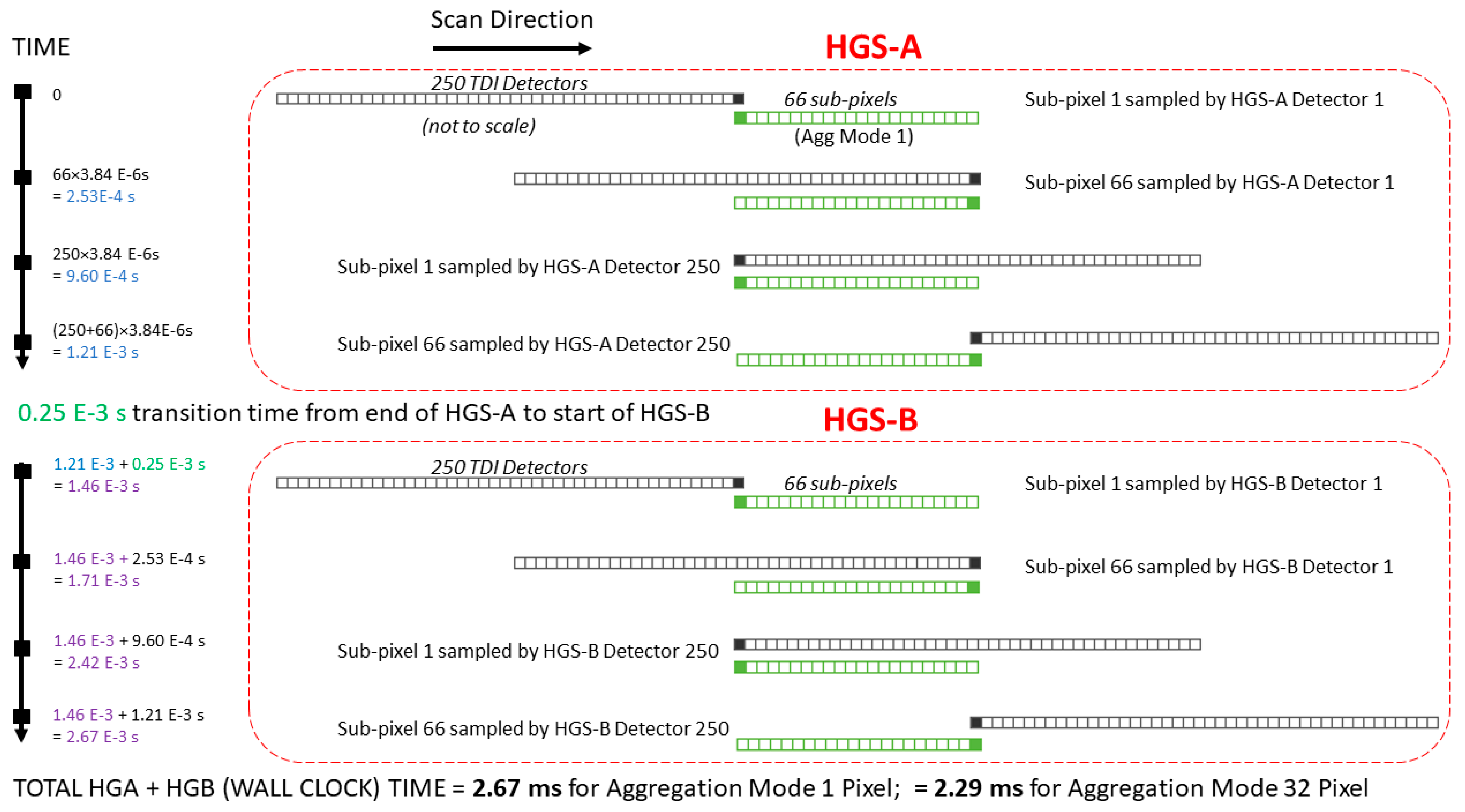
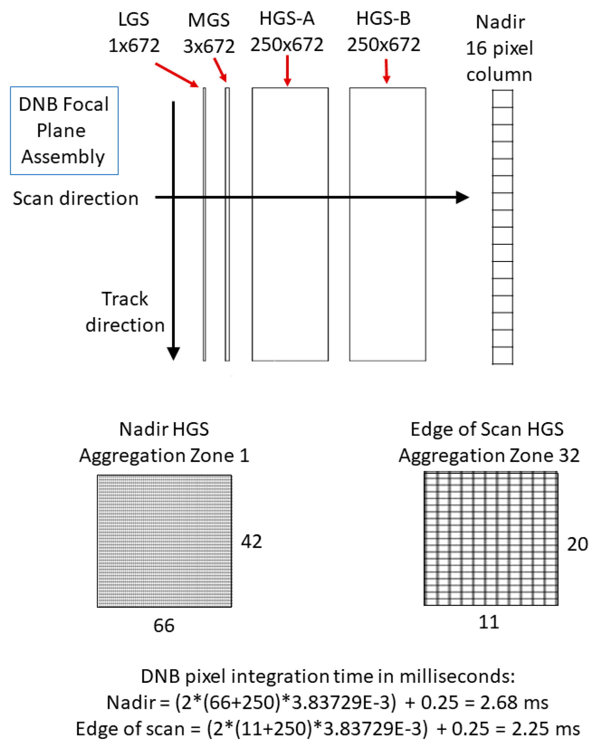
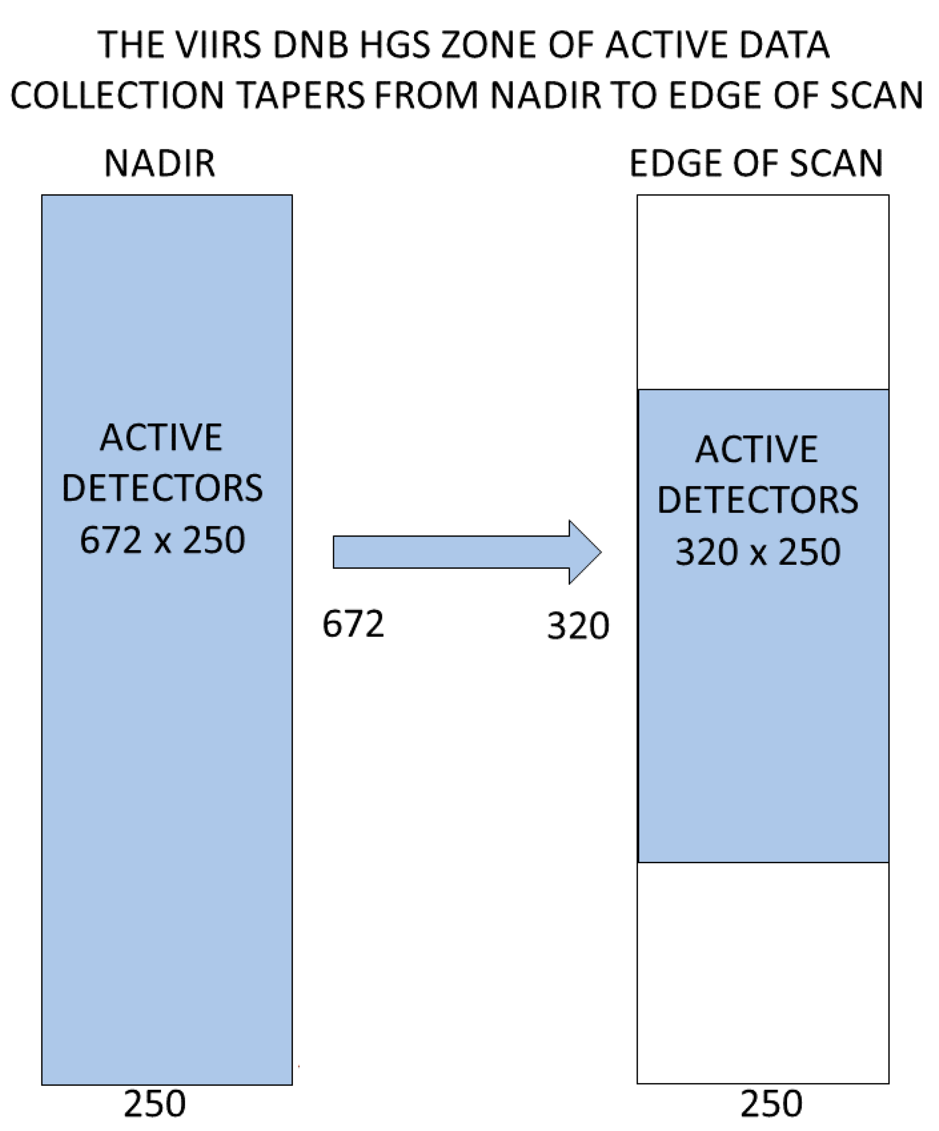
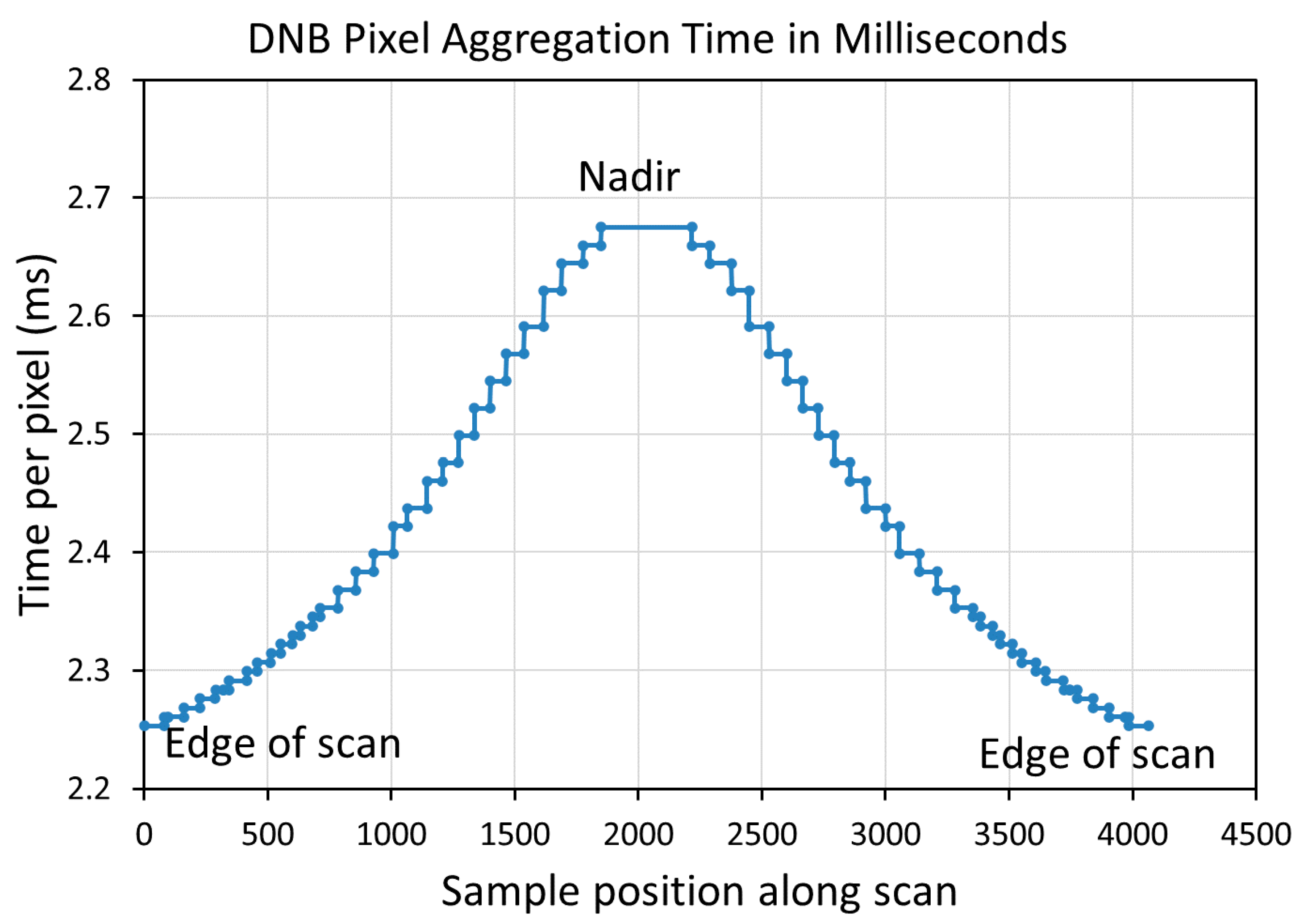
2.1. Calculation of DNB Pixel Dwell Times for High Gain Stage Data
2.2. Collection of High-Speed Camera Data of Individual Luminaires
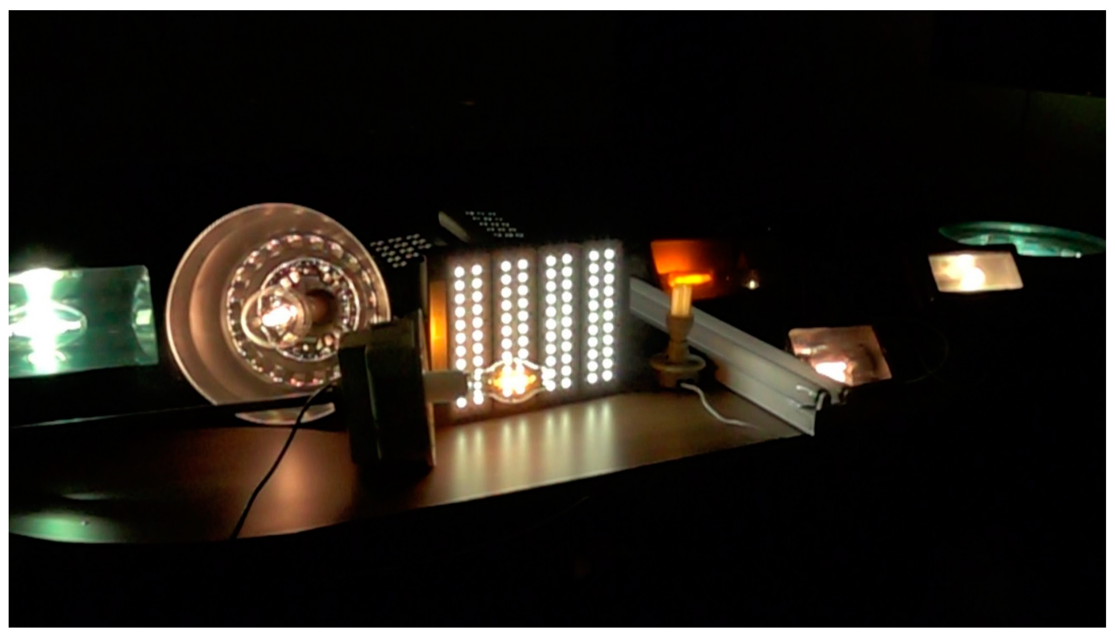
2.3. Collection of Flicker Data for Mixtures of Lights
2.4. Processing of the High-Speed Camera Data
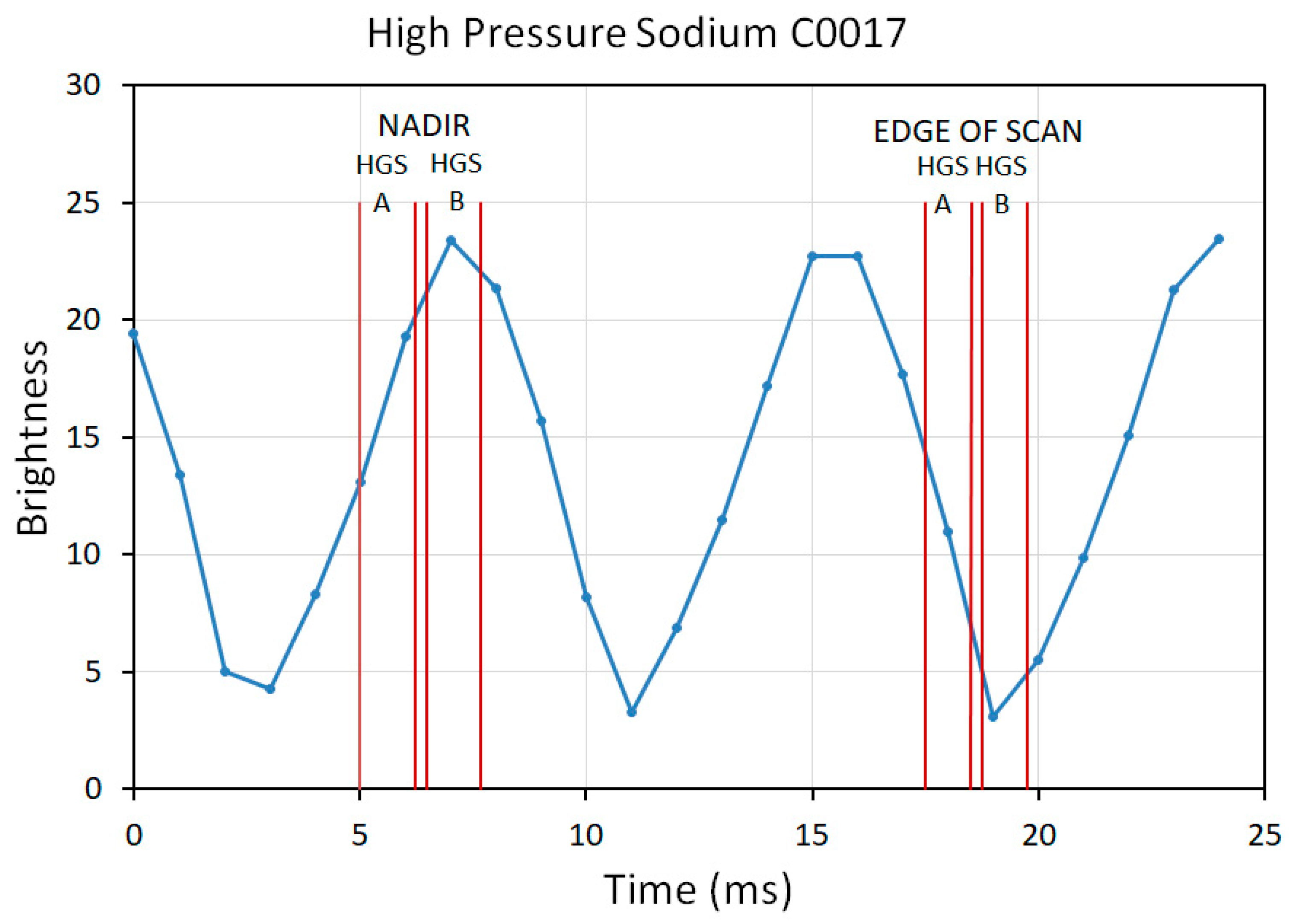
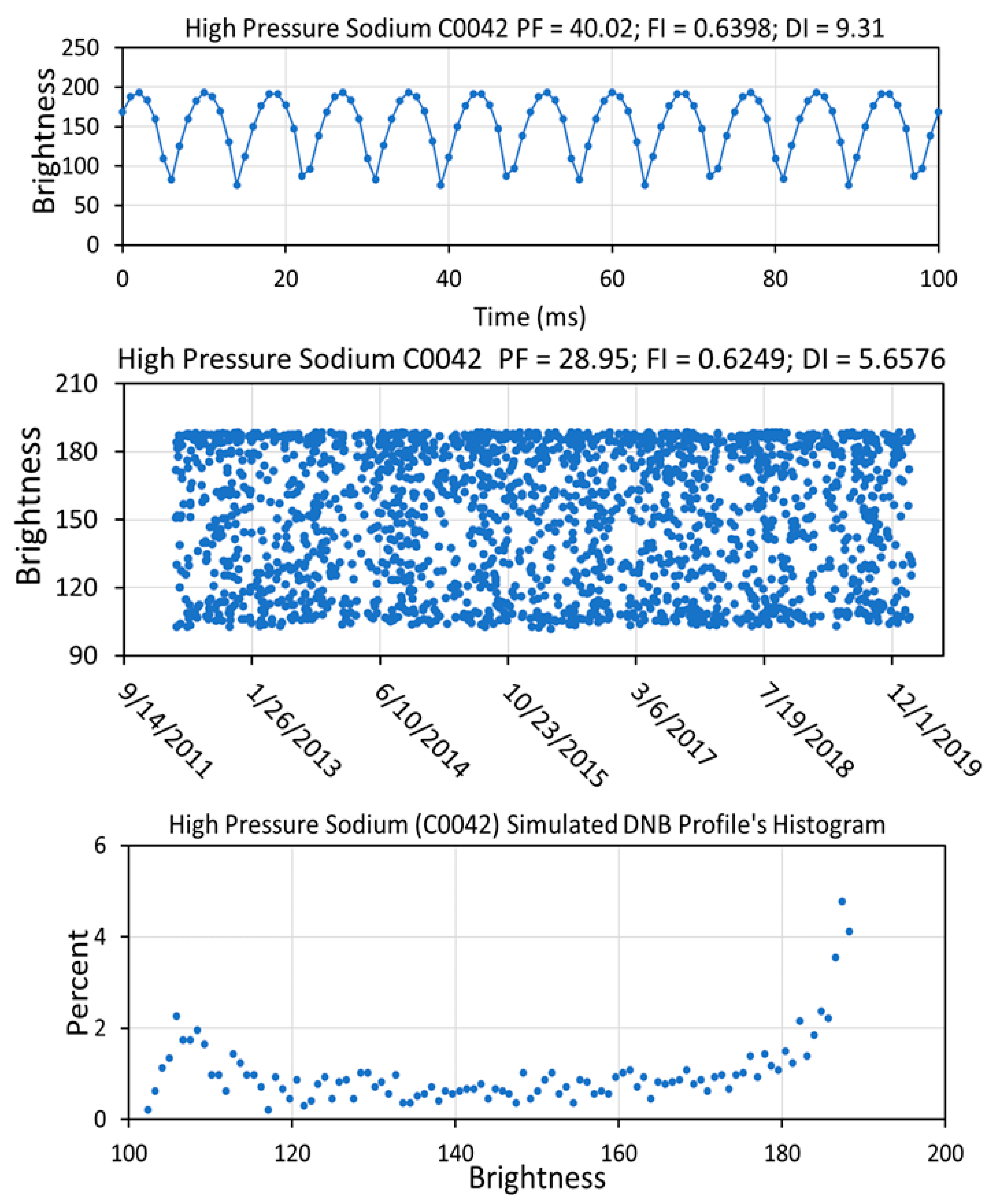
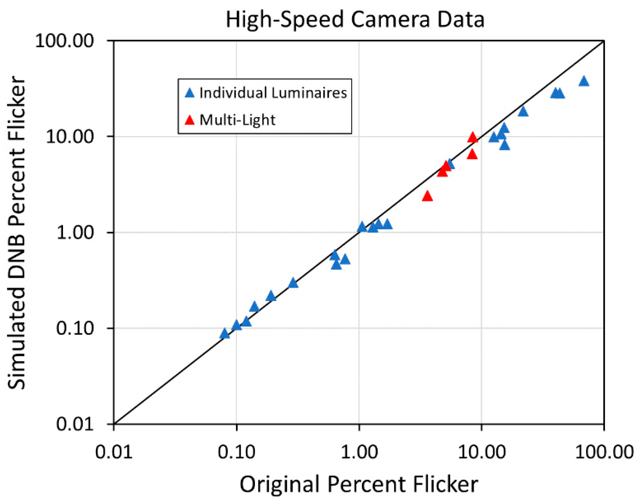
2.5. Simulation of DNB Temporal Profiles from the High-Speed Camera Data
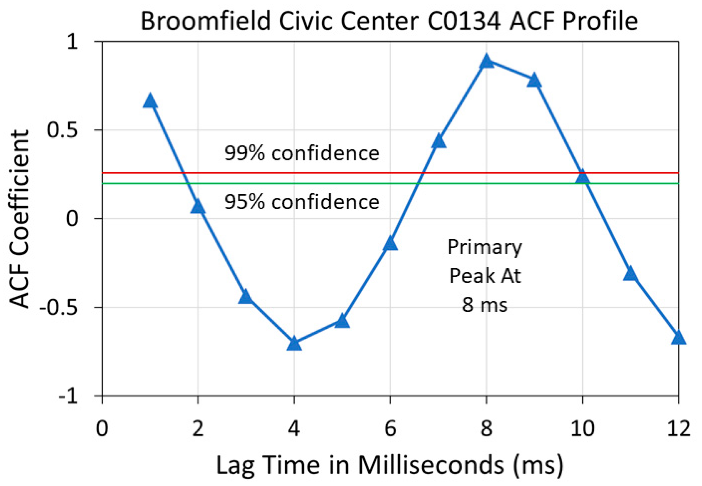
2.6. Examination of VIIRS DNB Temporal Profiles for Flicker Effects
3. Results
3.1. Re-Calculation of DNB Pixel Collection Times for HGS
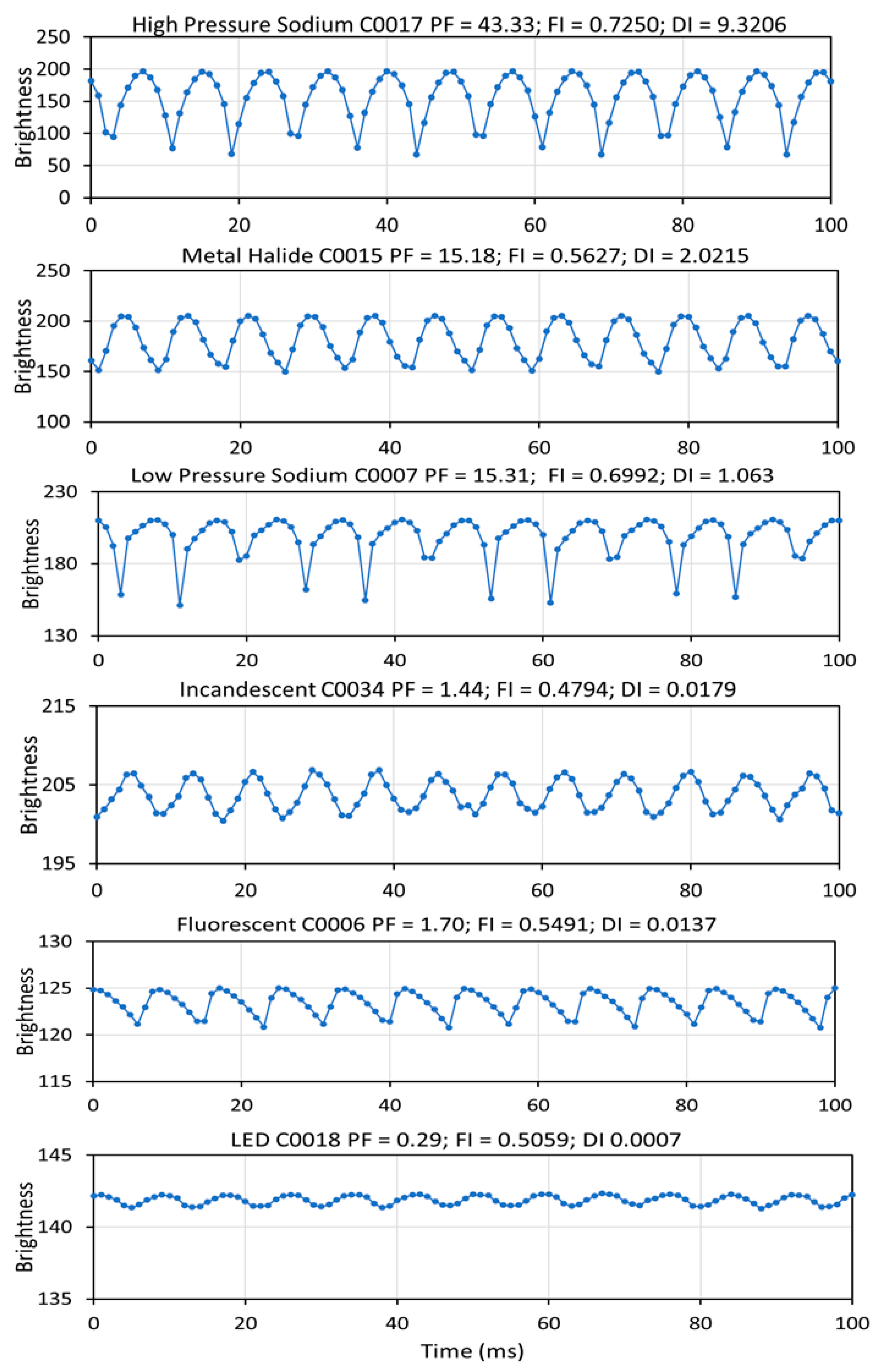
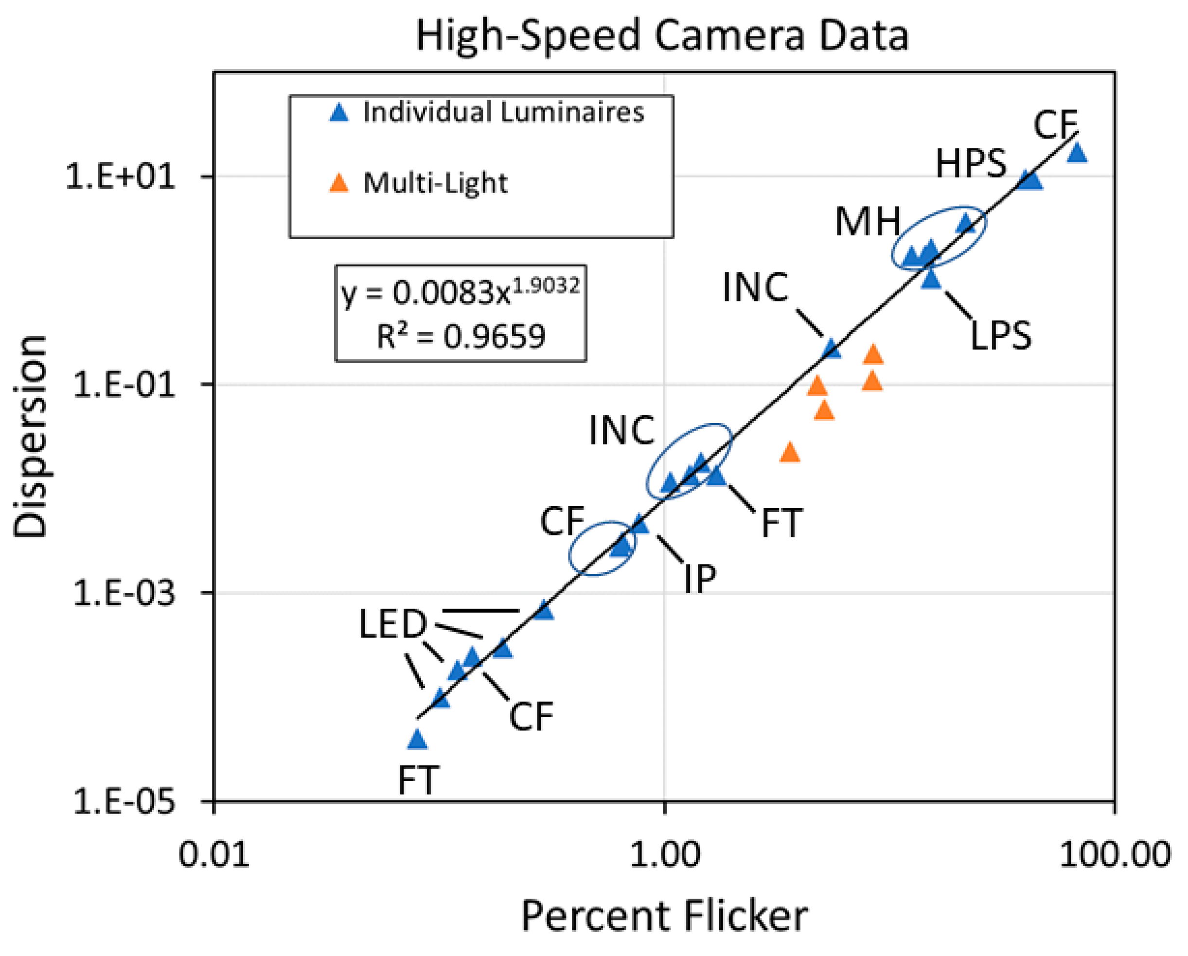
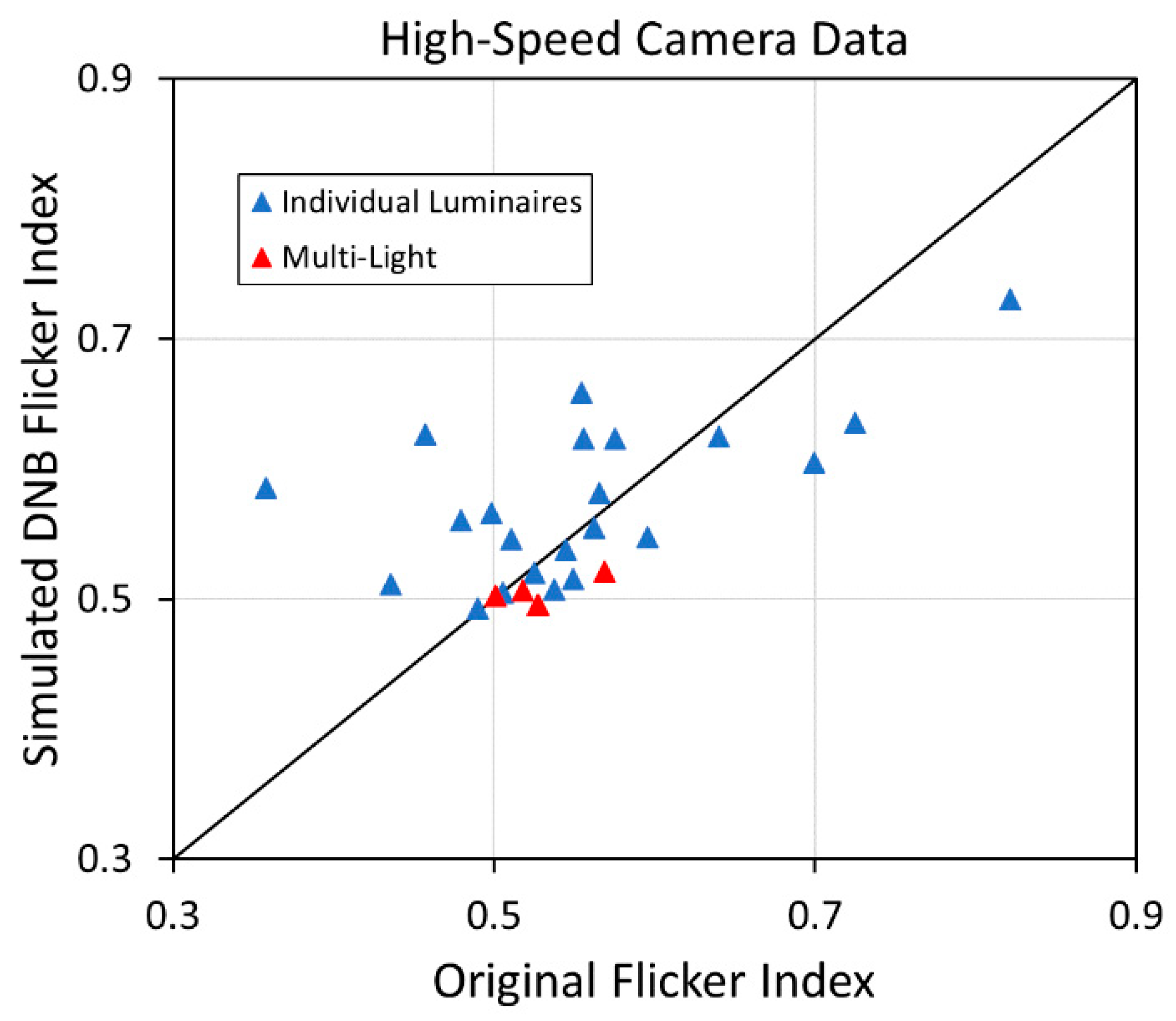
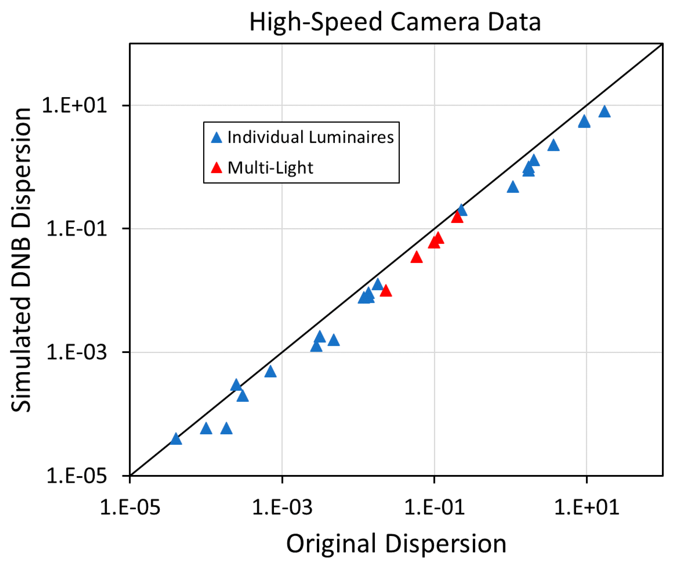
3.2. Results from High-Speed Camera Temporal Profiles for Individual Sources
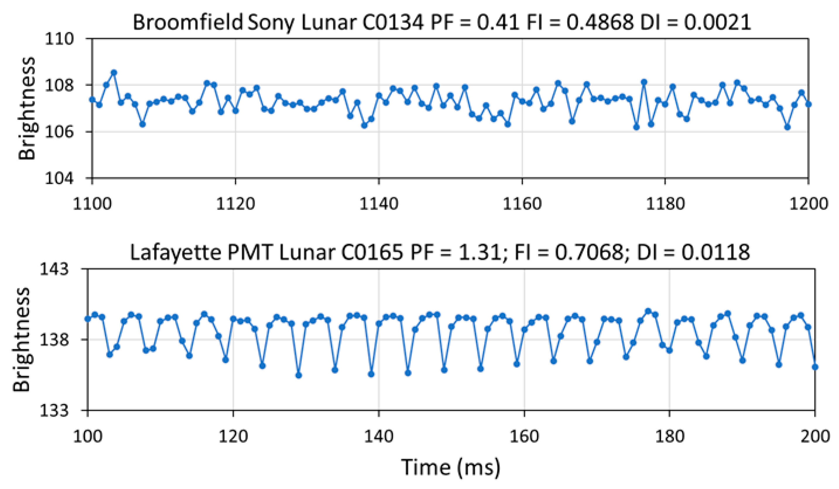
3.3. Results from Lunar Views
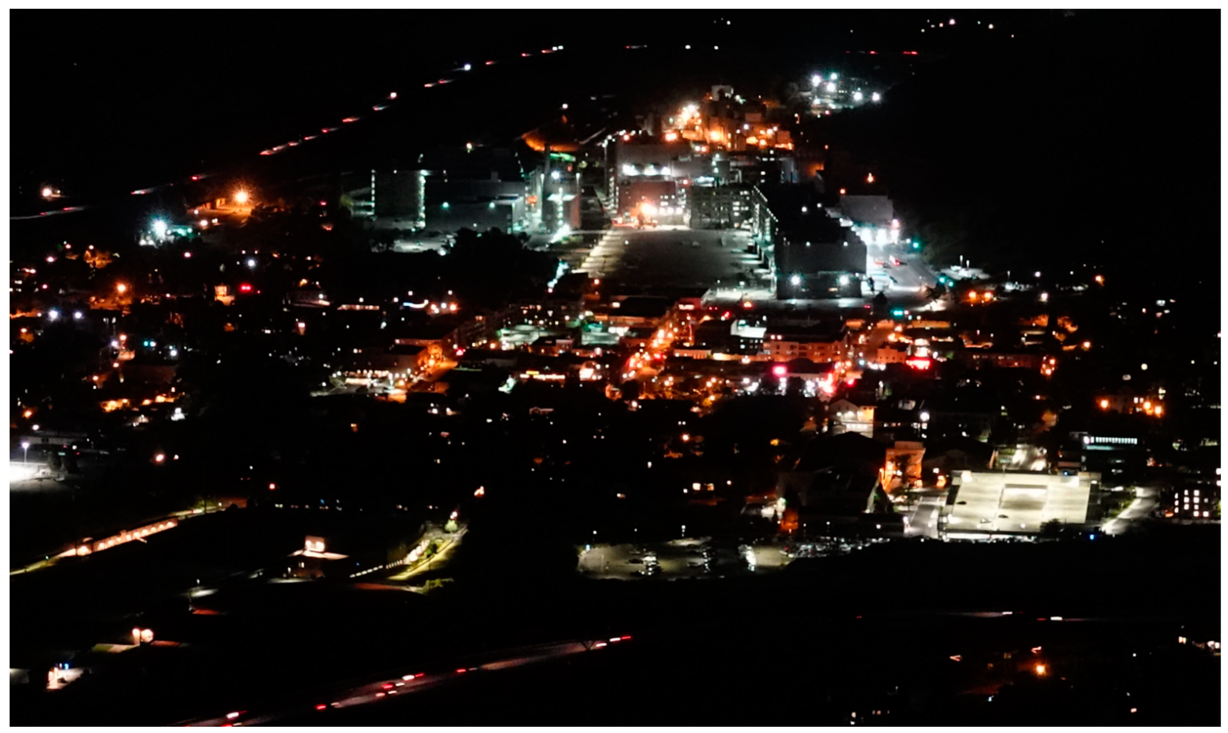
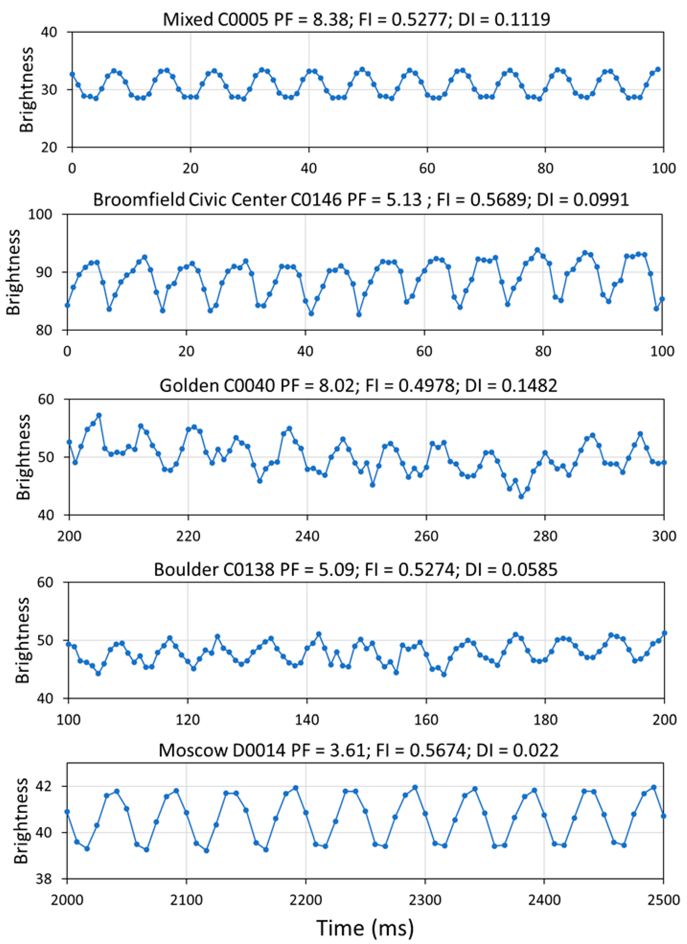
3.4. Results from High-Speed Camera Temporal Profiles for Multi-Light Collections
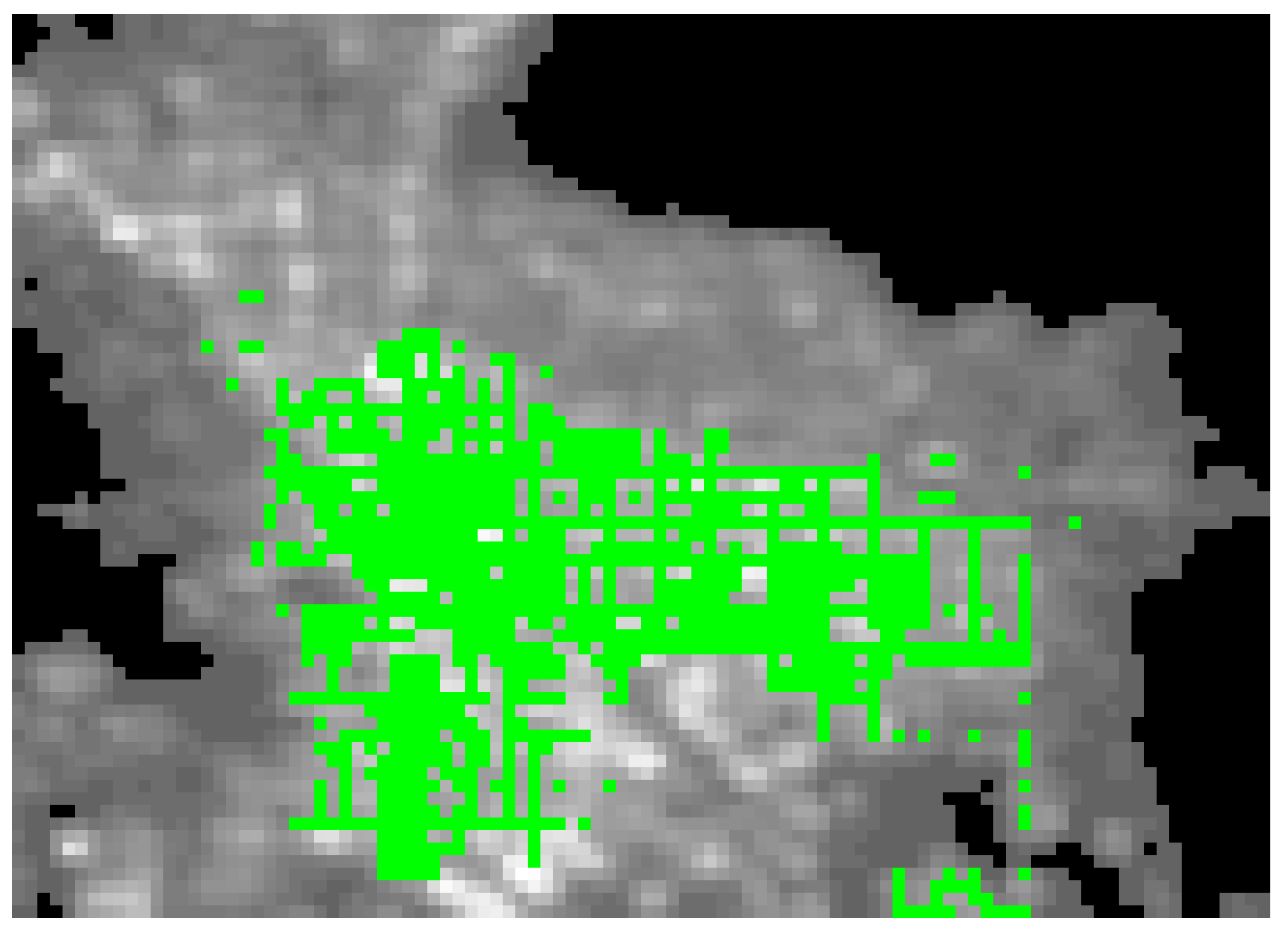
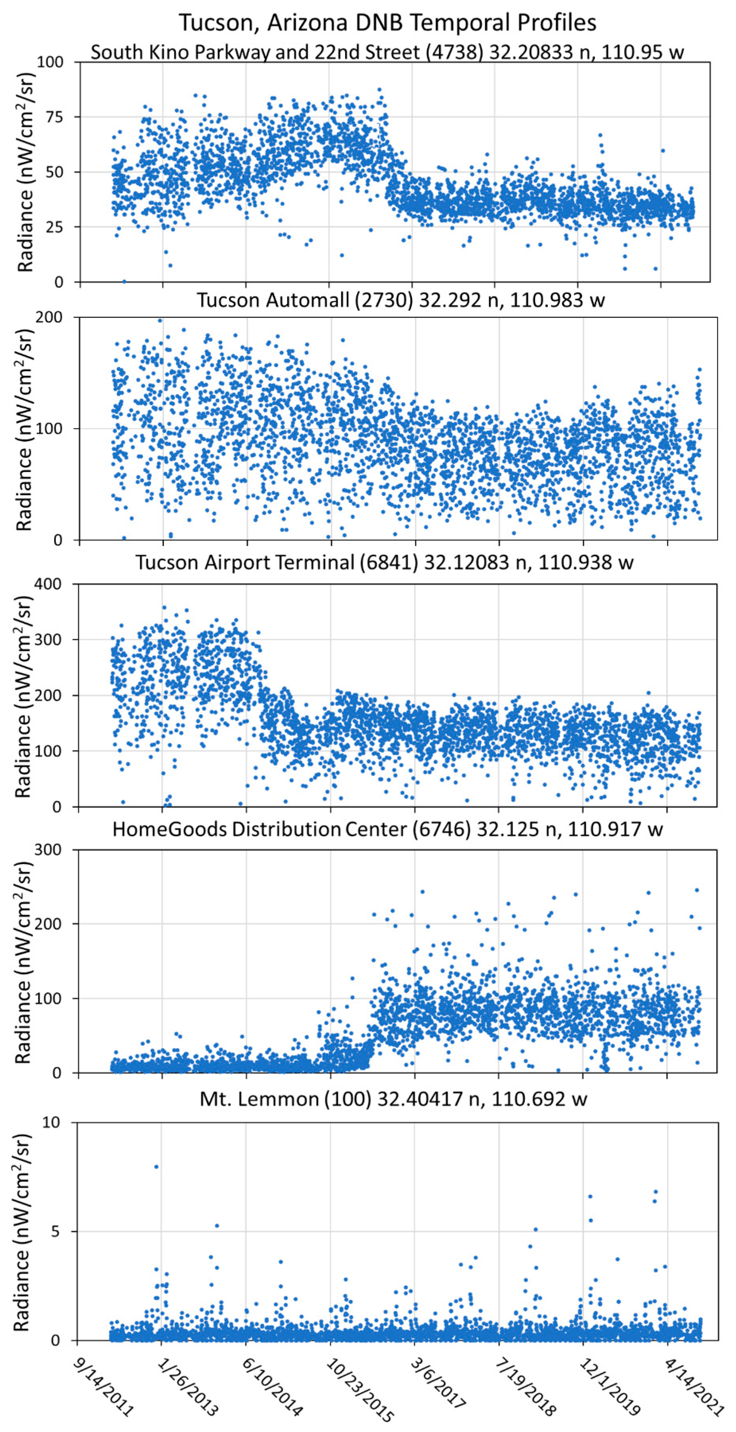
3.5. Examination of DNB Temporal Profiles of Tucson, Arizona
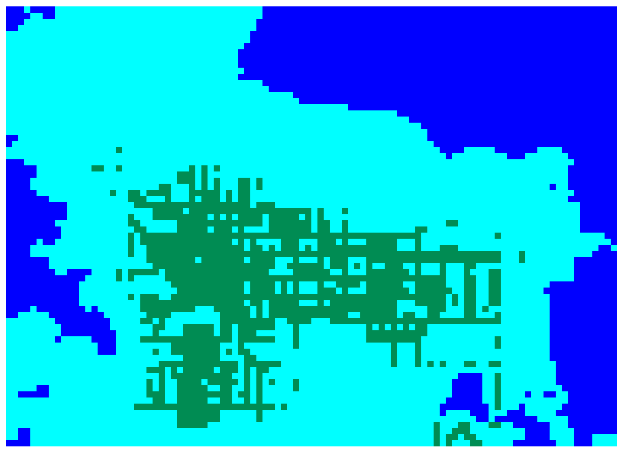
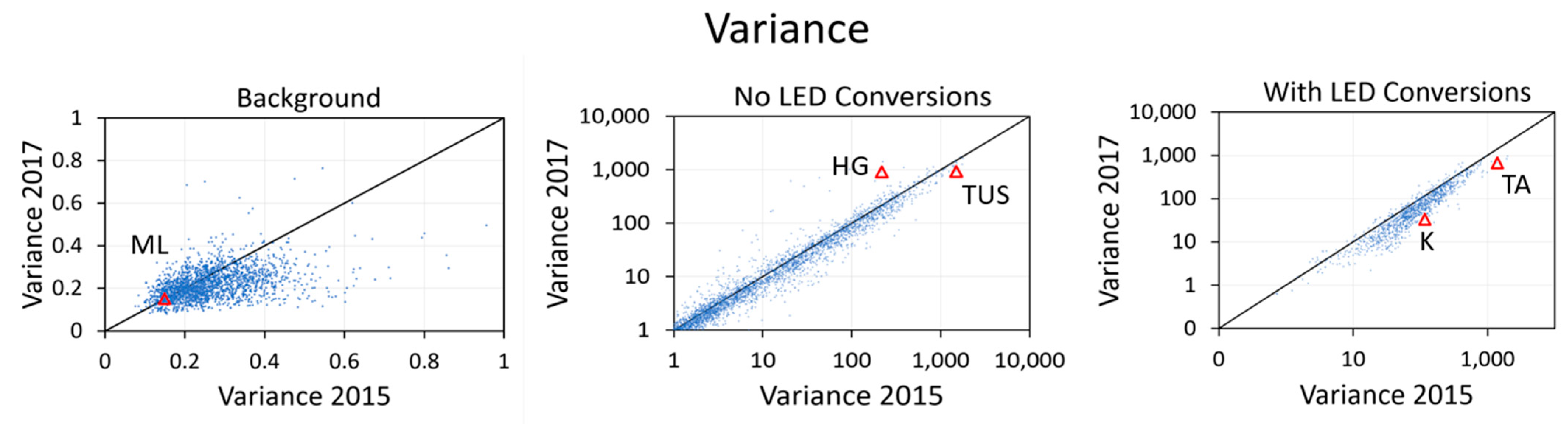
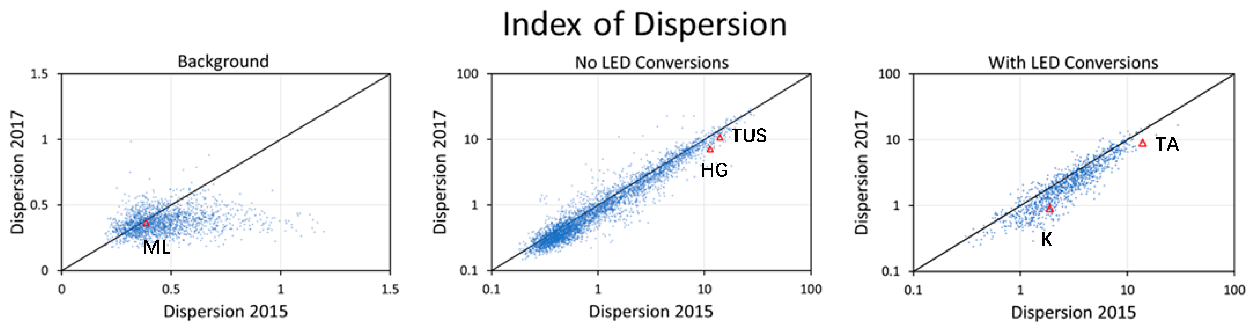
3.6. Examination of Annual Mean, Variance, and Dispersion across Tucson
4. Discussion
5. Conclusions
Author Contributions
Funding
Data Availability Statement
Acknowledgments
Conflicts of Interest
References
- Mirra, C. Flicker Measurement and Evaluation; Union Internationale d’Electrothermie, Group de Travail Perturbations: Paris, France, 1986. [Google Scholar]
- Fan, Y.H.; Wu, C.J.; Fan, C.C.; Chih, K.W.; Liao, L.D. A Novel Time Based Current Compensator for LED Back Light Modules. Key Eng. Mater. 2007, 364–366, 377–382. [Google Scholar] [CrossRef]
- Bartley, S.H. The neural determination of critical flicker frequency. J. Exp. Psychol. 1937, 21, 678. [Google Scholar] [CrossRef]
- Wilkins, A.; Veitch, J.; Lehman, B. LED lighting flicker and potential health concerns: IEEE standard PAR1789 update. In Proceedings of the 2010 IEEE Energy Conversion Congress and Exposition, ECCE, Atlanta, GA, USA, 12–16 September 2010; pp. 171–178. [Google Scholar] [CrossRef]
- Wilkins, A.J. Health and efficiency in lighting practice. Energy 1993, 18, 123–129. [Google Scholar] [CrossRef]
- Price, L.L.A. Can the Adverse Health Effects of Flicker from LEDs and Other Artificial Lighting Be Prevented? LEUKOS 2017, 13, 191–200. [Google Scholar] [CrossRef]
- Davis, J.; Hsieh, Y.-H.; Lee, H.-C. Humans perceive flicker artifacts at 500 Hz. Sci. Rep. 2015, 5, 7861. [Google Scholar] [CrossRef] [Green Version]
- IEEE Recommended Practices for Modulating Current in High-Brightness LEDs for Mitigating Health Risks to Viewers. IEEE-SA Standards Board, 26 March 2015. Available online: http://www.bio-licht.org/02_resources/info_ieee_2015_standards-1789.pdf (accessed on 5 March 2022).
- Takahashi, T.; Tsukahara, Y.; Nomura, M.; Matsuko, H. Pokemon Seizures. Neurol. J. Southeast Asia 1999, 4, 1–11. Available online: http://www.neurology-asia.org/articles/19991_001.pdf (accessed on 5 March 2022).
- Inger, R.; Bennie, J.; Davies, T.W.; Gaston, K.J. Potential biological and ecological effects of flickering artificial light. PLoS ONE 2014, 9, e98631. [Google Scholar] [CrossRef] [Green Version]
- Schakel, M.; Banerjee, K.; Bergen, T.; Blattner, P.; Bouroussis, C.; Dekker, P.; Klej, A.; Li, C.; Ootake, H.; Reiners, T.; et al. Guidance on the Measurement of Temporal Light Modulation of Light Sources and Lighting Systems; Technical Note 12; International Commission on Illumination: Vienna, Austria, 2021. [Google Scholar] [CrossRef]
- Baker, N.; Joint Polar Satellite System (JPSS); Visible Infrared Imaging Radiometer Suite (VIIRS); Sensor Data Records (SDR); Algorithm Theoretical Basis Document (ATBD). Goddard Space Flight Centre, Greenbelt Maryland, Ground Project Code, 474,474-00053. 22 April 2011. Available online: https://www.star.nesdis.noaa.gov/jpss/documents/ATBD/D0001-M01-S01-004_JPSS_ATBD_VIIRS-Geolocation_A.pdf (accessed on 7 March 2022).
- Elvidge, C.D.; Keith, D.M.; Tuttle, B.T.; Baugh, K.E. Spectral identification of lighting type and character. Sensors 2010, 10, 3961–3988. [Google Scholar] [CrossRef]
- Box, G.E.P.; Jenkins, G.M.; Reinsel, G.C. Autocorrelation Function and Spectrum of Stationary Processes. In Time Series Analysis; Wiley Online Library: Hoboken, NJ, USA, 2008; ISBN 9781118619193. [Google Scholar]
- Elvidge, C.D.; Hsu, F.-C.; Zhizhin, M.; Ghosh, T.; Taneja, J.; Bazilian, M. Indicators of electric power instability from satellite observed nighttime lights. Remote Sens. 2020, 12, 3194. [Google Scholar] [CrossRef]
- Hsu, F.; Zhizhin, M.; Ghosh, T.; Elvidge, C.; Taneja, J. The Annual Cycling of Nighttime Lights in India. Remote Sens. 2021, 13, 1199. [Google Scholar] [CrossRef]
- Ord, J.K.; Getis, A. Testing for local spatial autocorrelation in the presence of global autocorrelation. J. Reg. Sci. 2001, 41, 411–432. [Google Scholar] [CrossRef]
- The Illuminating Engineering Society of North America. The Lighting Handbook: Reference and Application, 10th ed.; IESNA: New York, NY, USA, 2011; 1328p. [Google Scholar]
- Selby, B. The index of dispersion as a test statistic. Biometrika 1965, 52, 627–629. [Google Scholar] [CrossRef]
- Kopp, T.J.; Thomas, W.; Heidinger, A.K.; Botambekov, D.; Frey, R.A.; Hutchison, K.D.; Iisager, B.D.; Brueske, K.; Reed, B. The VIIRS Cloud Mask: Progress in the First Year of S-NPP toward a Common Cloud Detection Scheme. J. Geophys. Res. Atmos. 2014, 119, 2441–2456. [Google Scholar] [CrossRef]
- Barentine, J.C.; Walker, C.E.; Kocifaj, M.; Kundracik, F.; Juan, A.; Kanemoto, J.; Monrad, C.K. Skyglow changes over Tucson, Arizona, resulting from a municipal LED street lighting conversion. J. Quant. Spectrosc. Radiat. Transf. 2018, 212, 10–23. [Google Scholar] [CrossRef] [Green Version]
- Barentine, J.C.; Kundracik, F.; Kocifaj, M.; Sanders, J.C.; Esquerdo, G.A.; Dalton, A.M.; Foott, B.; Grauer, A.; Tucker, S.; Kyba, C.C.M. Recovering the city street lighting fraction from skyglow measurements in a large-scale municipal dimming experiment. J. Quant. Spectrosc. Radiat. Transf. 2020, 253, 107120. [Google Scholar] [CrossRef]
- Kyba, C.C.M.; Ruby, A.; Kuechly, H.U.; Kinzey, B.; Miller, N.; Sanders, J.; Barentine, J.; Kleinodt, R.; Espey, B. Direct measurement of the contribution of street lighting to satellite observations of nighttime light emissions from urban areas. Light. Res. Technol. 2021, 53, 189–211. [Google Scholar] [CrossRef]
- Dick, R. Chapter 6—Harmonic Oscillators and Coherent States. In Advanced Quantum Mechanics; Springer: Berlin/Heidelberg, Germany, 2012. [Google Scholar]
- City of Tucson. HomeGoods Distribution Center Holds Grand Opening. 16 October 2016. Available online: https://www.tucsonaz.gov/ward-5/news/homegoods-distribution-center-holds-grand-opening (accessed on 28 November 2021).
- Dazhong, S.H.Z. Constant Current Driver for Semiconductor Lighting. Res. Prog. SSE Solid State Electron. 2006, 2. [Google Scholar]
- Wang, Z.; Román, M.O.; Kalb, V.L.; Miller, S.D.; Zhang, J.; Shrestha, R.M. Quantifying uncertainties in nighttime light retrievals from Suomi-NPP and NOAA-20 VIIRS Day/Night Band data. Remote Sens. Environ. 2021, 263, 112557. [Google Scholar] [CrossRef]
- Ryan, R.E.; Pagnutti, M.; Burch, K.; Leigh, L.; Ruggles, T.; Cao, C.; Aaron, D.; Blonski, S.; Helder, D. The Terra Vega active light source: A first step in a new approach to perform nighttime absolute radiometric calibrations and early results calibrating the VIIRS DNB. Remote Sens. 2019, 11, 710. [Google Scholar] [CrossRef] [Green Version]
- Cao, C.; Bai, Y. Quantitative analysis of VIIRS DNB nightlight point source for light power estimation and stability monitoring. Remote Sens. 2014, 6, 11915–11935. [Google Scholar] [CrossRef] [Green Version]
- Elvidge, C.D.; Baugh, K.; Zhizhin, M.; Hsu, F.C.; Ghosh, T. VIIRS night-time lights. Int. J. Remote Sens. 2017, 38, 5860–5879. [Google Scholar] [CrossRef]
- Elvidge, C.D.; Zhizhin, M.; Ghosh, T.; Hsu, F.-C.; Taneja, J. Annual time series of global VIIRS nighttime lights derived from monthly averages: 2012 to 2019. Remote Sens. 2021, 13, 922. [Google Scholar] [CrossRef]
- Weinold, M. A long overdue end to flicker: The 2020 EU lighting efficiency regulations. Camb. J. Sci. Policy 2020, 1, e0628620899. [Google Scholar]
- Bullough, J.D. The blue-light hazard: A review. J. Illum. Eng. Soc. 2000, 29, 6–14. [Google Scholar] [CrossRef]
- Bullough, J.D.; Bierman, A.; Rea, M.S. Evaluating the blue-light hazard from solid state lighting. Int. J. Occup. Saf. Ergon. 2019, 25, 311–320. [Google Scholar] [CrossRef]


| Luminaire Type | Designation | Sample | Manufacturer | Model | Wattage |
|---|---|---|---|---|---|
| Metal Halide | Ceramic Metal Halide | C0009 | Sylvania | MetalARC Mp 100/U/MED | 100 |
| Metal Halide | C0012 | EMCO Lighting | ERA20-3H SO-89193 | 175 | |
| Metal Halide | C0015 | Philips | MP400/BU/PS Kr85 | 400 | |
| Metal Halide RAB | C0016 | RAB | RAB LMH250PS | 250 | |
| High Pressure Sodium | HPS | C0017 | Sylvania | LU150/55/ECO | 175 |
| HPS | C0041 | General Electric | Lucalox | 100 | |
| Low Pressure Sodium | LPS | C0007 | Osram | N068 80X Great Britain | 18 |
| Fluorescent | 4 foot tube pair | C0006 | Philips | Alto F40T/C50 Sumpreme | 40 |
| Fluorescent ceiling | C0035 | Philips | Alto-II F32T8/Tl841 800 series | 32 | |
| Compact Fluorescent | C0028 | BFLG | 13 | 13 | |
| Compact Fluorescent | C0031 | Greenlight | 13W/ELS-M/1 | 13 | |
| Compact Fluorescent | C0032 | TCP | ESN11 | 11 | |
| Incandescent | Incandescent | C0014 | |||
| Incandescent | C0027 | Sylvania | Capsylite FL-tugsten-halogen | 45 | |
| Incandescent | C0034 | Soft White | 60 | ||
| LED | LED | C0018 | PLT Solutions | PLT-11557 | 300 |
| LED 4000 K | C0020 | LeoTEK | Beta | 100 | |
| LED 3000 K | C0022 | LeoTEK | Beta | 100 | |
| LED | C0026 | Lithonia | DSXPG | 51 | |
| iphone | C0036 | Apple | iPhone Xr MT472LL/A | ? |
| Aggregation Mode from Nadir | Number of Sub-pixels per Pixel | Number of Pixels per Mode | Time per Pixel (s) HGS-A | Time on HGS A-B Gap (s) | Time per Pixel (s) HGS-B | Total Time per DNB Pixel (s) | |
|---|---|---|---|---|---|---|---|
| Track Direction | Scan Direction | ||||||
| 1 | 42 | 66 | 184 | 1.21E-03 | 2.50E-04 | 1.21E-03 | 2.68E-03 |
| 2 | 42 | 64 | 72 | 1.20E-03 | 2.50E-04 | 1.20E-03 | 2.66E-03 |
| 3 | 41 | 62 | 88 | 1.20E-03 | 2.50E-04 | 1.20E-03 | 2.64E-03 |
| 4 | 40 | 59 | 72 | 1.19E-03 | 2.50E-04 | 1.19E-03 | 2.62E-03 |
| 5 | 39 | 55 | 80 | 1.17E-03 | 2.50E-04 | 1.17E-03 | 2.59E-03 |
| 6 | 38 | 52 | 72 | 1.16E-03 | 2.50E-04 | 1.16E-03 | 2.57E-03 |
| 7 | 37 | 49 | 64 | 1.15E-03 | 2.50E-04 | 1.15E-03 | 2.54E-03 |
| 8 | 36 | 46 | 64 | 1.14E-03 | 2.50E-04 | 1.14E-03 | 2.52E-03 |
| 9 | 35 | 43 | 64 | 1.12E-03 | 2.50E-04 | 1.12E-03 | 2.50E-03 |
| 10 | 34 | 40 | 64 | 1.11E-03 | 2.50E-04 | 1.11E-03 | 2.48E-03 |
| 11 | 33 | 38 | 64 | 1.11E-03 | 2.50E-04 | 1.11E-03 | 2.46E-03 |
| 12 | 32 | 35 | 80 | 1.09E-03 | 2.50E-04 | 1.09E-03 | 2.44E-03 |
| 13 | 31 | 33 | 56 | 1.09E-03 | 2.50E-04 | 1.09E-03 | 2.42E-03 |
| 14 | 30 | 30 | 80 | 1.07E-03 | 2.50E-04 | 1.07E-03 | 2.40E-03 |
| 15 | 29 | 28 | 72 | 1.07E-03 | 2.50E-04 | 1.07E-03 | 2.38E-03 |
| 16 | 28 | 26 | 72 | 1.06E-03 | 2.50E-04 | 1.06E-03 | 2.37E-03 |
| 17 | 27 | 24 | 72 | 1.05E-03 | 2.50E-04 | 1.05E-03 | 2.35E-03 |
| 18 | 27 | 23 | 32 | 1.05E-03 | 2.50E-04 | 1.05E-03 | 2.35E-03 |
| 19 | 26 | 22 | 48 | 1.04E-03 | 2.50E-04 | 1.04E-03 | 2.34E-03 |
| 20 | 26 | 21 | 32 | 1.04E-03 | 2.50E-04 | 1.04E-03 | 2.33E-03 |
| 21 | 25 | 20 | 48 | 1.04E-03 | 2.50E-04 | 1.04E-03 | 2.32E-03 |
| 22 | 25 | 19 | 40 | 1.03E-03 | 2.50E-04 | 1.03E-03 | 2.31E-03 |
| 23 | 24 | 18 | 56 | 1.03E-03 | 2.50E-04 | 1.03E-03 | 2.31E-03 |
| 24 | 24 | 17 | 40 | 1.02E-03 | 2.50E-04 | 1.02E-03 | 2.30E-03 |
| 25 | 23 | 16 | 72 | 1.02E-03 | 2.50E-04 | 1.02E-03 | 2.29E-03 |
| 26 | 23 | 15 | 24 | 1.02E-03 | 2.50E-04 | 1.02E-03 | 2.28E-03 |
| 27 | 22 | 15 | 32 | 1.02E-03 | 2.50E-04 | 1.02E-03 | 2.28E-03 |
| 28 | 22 | 14 | 64 | 1.01E-03 | 2.50E-04 | 1.01E-03 | 2.28E-03 |
| 29 | 21 | 13 | 64 | 1.01E-03 | 2.50E-04 | 1.01E-03 | 2.27E-03 |
| 30 | 21 | 12 | 64 | 1.01E-03 | 2.50E-04 | 1.01E-03 | 2.26E-03 |
| 31 | 20 | 12 | 16 | 1.01E-03 | 2.50E-04 | 1.01E-03 | 2.26E-03 |
| 32 | 20 | 11 | 80 | 1.00E-03 | 2.50E-04 | 1.00E-03 | 2.25E-03 |
| Total | 2032 | 7.71E-02 | |||||
| Luminaires | Number | % Flicker | Flicker Index | Dispersion | Flicker Hz | SDNB % Flicker | SDNB Flicker Index | SDNB Dispersion |
|---|---|---|---|---|---|---|---|---|
| Compact Fluorescent | C0028 | 68.12 | 0.8216 | 17.1248 | 120 | 38.59 | 0.7303 | 8.0688 |
| High Pressure Sodium | C0017 | 43.33 | 0.7250 | 9.3200 | 120 | 28.69 | 0.6356 | 5.4270 |
| High Pressure Sodium | C0042 | 40.02 | 0.6398 | 9.3078 | 120 | 28.95 | 0.6249 | 5.6576 |
| Metal halide | C0012 | 21.71 | 0.5656 | 3.6492 | 120 | 18.49 | 0.5816 | 2.3106 |
| Low Pressure Sodium | C0007 | 15.31 | 0.6992 | 1.0630 | 120 | 8.25 | 0.6051 | 0.4863 |
| Metal Halide | C0015 | 15.18 | 0.5627 | 2.0215 | 120 | 12.40 | 0.5550 | 1.3042 |
| Ceramic metal Halide | C0009 | 14.40 | 0.5754 | 1.7200 | 120 | 10.73 | 0.6237 | 1.0180 |
| Metal Halide RAB | C0016 | 12.51 | 0.5956 | 1.7166 | 120 | 9.96 | 0.5474 | 0.8887 |
| Incandescent | C0027 | 5.47 | 0.5108 | 0.2264 | 60 | 5.26 | 0.5464 | 0.2031 |
| Fluorescent | C0006 | 1.70 | 0.5491 | 0.0137 | 120 | 1.23 | 0.5152 | 0.0080 |
| Incandescent | C0034 | 1.44 | 0.4794 | 0.0179 | 120 | 1.23 | 0.5604 | 0.0128 |
| Incandescent dual | C0033 | 1.30 | 0.4986 | 0.0135 | 120 | 1.14 | 0.5661 | 0.0093 |
| Incandescent | C0014 | 1.06 | 0.5379 | 0.0118 | 120 | 1.16 | 0.5075 | 0.0077 |
| iphone flashlight | C0036 | 0.77 | 0.4574 | 0.0047 | 0 | 0.53 | 0.6268 | 0.0016 |
| Compact Fluorescent | C0031 | 0.65 | 0.5561 | 0.0031 | 120 | 0.47 | 0.6230 | 0.0018 |
| Compact Fluorescent | C0032 | 0.63 | 0.3580 | 0.0028 | 120 | 0.59 | 0.5852 | 0.0013 |
| LED | C0018 | 0.29 | 0.5059 | 0.0007 | 120 | 0.30 | 0.5049 | 0.0005 |
| LED 4000 K | C0020 | 0.19 | 0.4897 | 0.0003 | 120 | 0.22 | 0.4930 | 0.0002 |
| Compact Fluorescent | C0011 | 0.14 | 0.5450 | 0.0003 | 120 | 0.17 | 0.5378 | 0.0003 |
| LED | C0026 | 0.12 | 0.5250 | 0.0002 | 120 | 0.12 | 0.5201 | 0.0001 |
| LED 3000 K | C0022 | 0.10 | 0.4360 | 0.0001 | 120 | 0.11 | 0.5117 | 0.0001 |
| Fluorescent Ceiling | C0035 | 0.08 | 0.5547 | 0.00004 | 120 | 0.09 | 0.6592 | 0.00004 |
| Observed Scene | Number | % Flicker | Flicker Index | Dispersion | Flicker Hz | DNB % Flicker | DNB Flicker Index | DNB Dispersion |
|---|---|---|---|---|---|---|---|---|
| Table Multilights | C0005 | 8.38 | 0.5277 | 0.1119 | 120 | 6.67 | 0.4953 | 0.072 |
| Golden Panorama | C0040 | 8.43 | 0.5178 | 0.1972 | 120 | 9.92 | 0.5069 | 0.1581 |
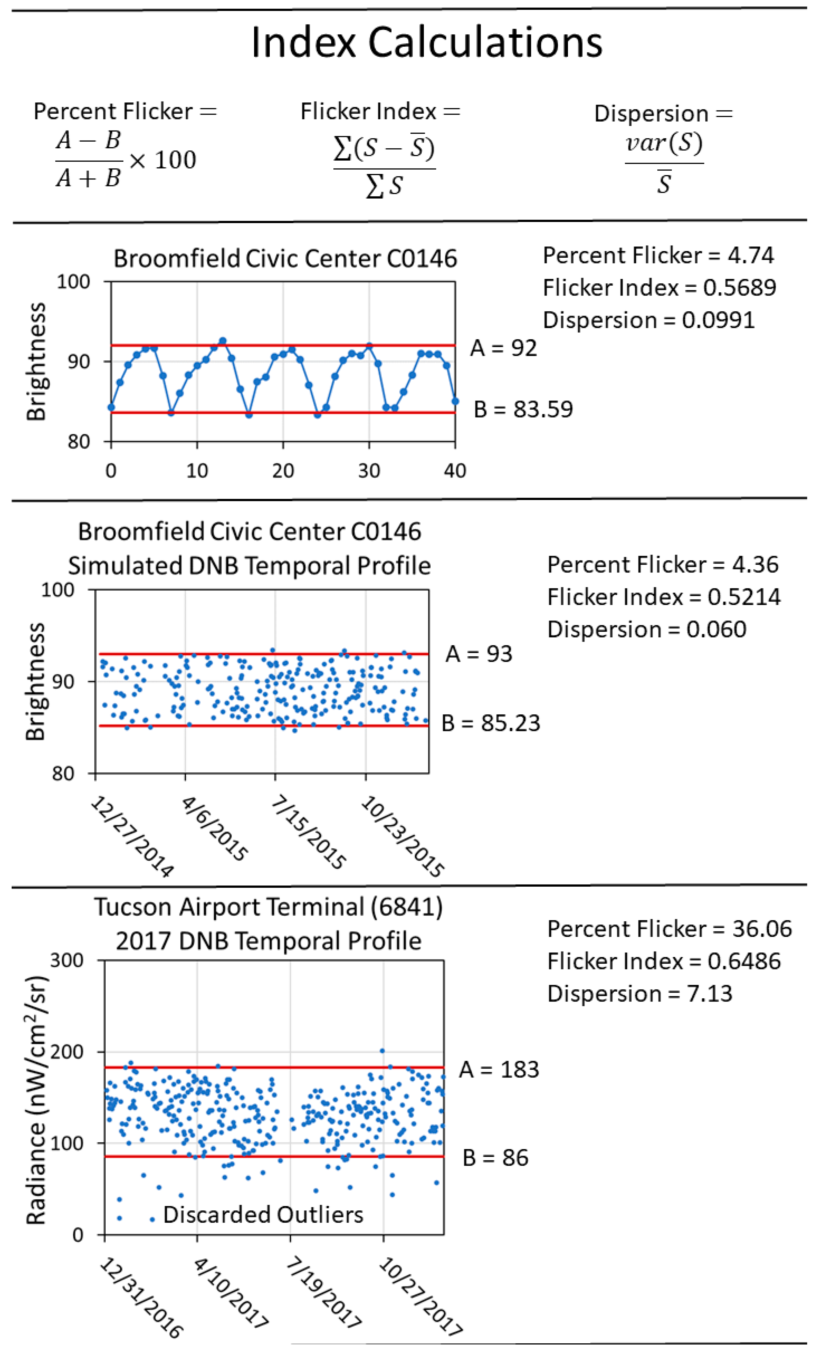
| Broomfield Civic Center | C0146 | 4.79 | 0.5689 | 0.0991 | 120 | 4.36 | 0.5214 | 0.06 |
| Boulder Panorama | C0138 | 5.09 | 0.5274 | 0.0585 | 120 | 4.99 | 0.4956 | 0.0349 |
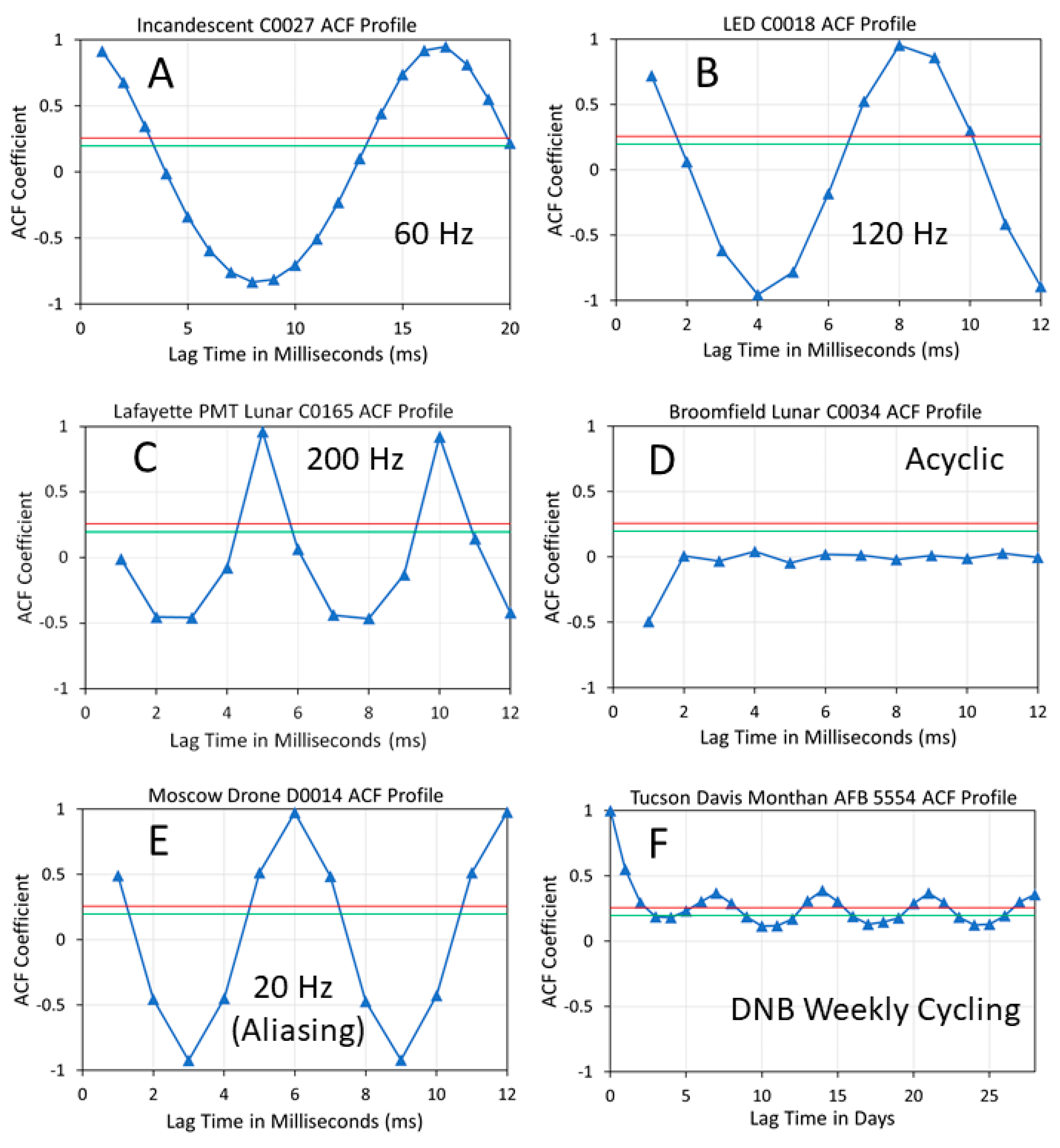
| Moscow Drone | D0014 | 3.61 | 0.5008 | 0.0228 | 100 | 2.45 | 0.5026 | 0.0101 |
| Location | Cell Number | Reference Year | Ref. % Flicker | Ref. Flicker Index | Ref. Dispersion | 2017 % Flicker | 2017 Flicker Index | 2017 Dispersion | LED Conversions |
|---|---|---|---|---|---|---|---|---|---|
| S. Kino Parkway and 22nd | 4738 | 2015 | 21.21 | 0.5797 | 1.88 | 23.29 | 0.5148 | 0.91 | 61 |
| Automall | 2730 | 2015 | 63.77 | 0.677 | 13.92 | 59.09 | 0.6725 | 9.01 | 29 |
| HomeGoods Distribution Center | 6746 | 2014 | 99.99 | 0.6175 | 4.15 | 41.63 | 0.5644 | 10.87 | 0 |
| Airport terminal | 6841 | 2013 | 22.59 | 0.657 | 15.17 | 36.06 | 0.6457 | 7.13 | 0 |
| Mt. Lemmon | 100 | 2015 | 99.97 | 0.6426 | 0.422 | 99.96 | 0.6554 | 0.404 | 0 |
Publisher’s Note: MDPI stays neutral with regard to jurisdictional claims in published maps and institutional affiliations. |
© 2022 by the authors. Licensee MDPI, Basel, Switzerland. This article is an open access article distributed under the terms and conditions of the Creative Commons Attribution (CC BY) license (https://creativecommons.org/licenses/by/4.0/).
Share and Cite
Elvidge, C.D.; Zhizhin, M.; Keith, D.; Miller, S.D.; Hsu, F.C.; Ghosh, T.; Anderson, S.J.; Monrad, C.K.; Bazilian, M.; Taneja, J.; et al. The VIIRS Day/Night Band: A Flicker Meter in Space? Remote Sens. 2022, 14, 1316. https://doi.org/10.3390/rs14061316
Elvidge CD, Zhizhin M, Keith D, Miller SD, Hsu FC, Ghosh T, Anderson SJ, Monrad CK, Bazilian M, Taneja J, et al. The VIIRS Day/Night Band: A Flicker Meter in Space? Remote Sensing. 2022; 14(6):1316. https://doi.org/10.3390/rs14061316
Chicago/Turabian StyleElvidge, Christopher D., Mikhail Zhizhin, David Keith, Steven D. Miller, Feng Chi Hsu, Tilottama Ghosh, Sharolyn J. Anderson, Christian K. Monrad, Morgan Bazilian, Jay Taneja, and et al. 2022. "The VIIRS Day/Night Band: A Flicker Meter in Space?" Remote Sensing 14, no. 6: 1316. https://doi.org/10.3390/rs14061316
APA StyleElvidge, C. D., Zhizhin, M., Keith, D., Miller, S. D., Hsu, F. C., Ghosh, T., Anderson, S. J., Monrad, C. K., Bazilian, M., Taneja, J., Sutton, P. C., Barentine, J., Kowalik, W. S., Kyba, C. C. M., Pack, D. W., & Hammerling, D. (2022). The VIIRS Day/Night Band: A Flicker Meter in Space? Remote Sensing, 14(6), 1316. https://doi.org/10.3390/rs14061316