Random Forest Classification of Land Use, Land-Use Change and Forestry (LULUCF) Using Sentinel-2 Data—A Case Study of Czechia

Abstract

Land use, land-use change and forestry (LULUCF) is a greenhouse gas inventory sector that evaluates greenhouse gas changes in the atmosphere from land use and land-use change. This study focuses on the development of a Sentinel-2 data classification according to the LULUCF requirements on the cloud-based platform Google Earth Engine (GEE). The methods are tested in selected larger territorial regions (two Czech NUTS 2 units) using data collected in 2018. The Random Forest method was used for classification. In terms of classification accuracy, a combination of these parameters was tested: The Number of Trees (NT), the Variables per Split (VPS) and the Bag Fraction (BF). A total of 450 combinations of different parameters were tested. The highest accuracy classification with an overall accuracy = 89.1% and Cohen’s Kappa = 0.84 had the following combination: NT = 150, VPS = 3 and BF = 0.1. For classification purposes, a mosaic was created using the median method. The resulting mosaic consisted of all Sentinel-2 bands in 10 and 20 m spatial resolution. Altitude values derived from SRTM and NDVI variance values were also included in the classification. These added bands were the most significant in terms of Gini importance.

1. Introduction

The land cover/land-use change (LCLUC) program is one of the most important sources of information on the development of global environmental change. LCLUC forms the primary source of data for numerous mathematical models that seek to define future development scenarios in many areas of the environment, including climate change [1,2]. The UN Secretariat on Climate Change and the adopted Paris Agreements under the United States Framework Convention on Climate Change (UNFCCC) have declared the LCLUCs monitoring to be highly relevant, as LCLUCs have a significant impact on climate change and the global carbon cycle. For these purposes, the binding regulation is provided for the inventory and reporting of relevant land use classes, so-called LULUCF—land use, land-use change and forestry (see Decision 529/2013/EU, European Commission 2013). LULUCF information is collected and reported on an international scale and is one of the main input data sources for climate change modeling and GHG (greenhouse gas) emission estimates within the IPCC (Intergovernmental Panel on Climate Change).

The development of international agreements on climate and climate policy has been shaping the role of LULUCF. Researchers are increasingly developing sophisticated research strategies to represent the global dimension of land use and assess its impact on climate mitigation [3]. Full LULUCF integration fits well with ongoing international efforts to integrate forests and other aspects into the climate policy framework, e.g., the context of REDD+ (Reduced Emissions from Deforestation and Forest Degradation) [4,5,6]. Standardized methods and accurate and harmonized LULUCF data are a key factor in accounting and evaluating the changes over a long period and modeling climate change with predictive scenarios [7,8]. Earth observation (EO) is an effective and promising tool for monitoring LCLUC [9,10]. The wide use of satellite data is currently possible mainly due to the creation of freely available archives of satellite images from different missions (e.g., Landsat and the Copernicus program). The Copernicus program has brought new possibilities to EO. ESA is launching new satellite missions called Sentinels specifically for the operational needs of the Copernicus program. The Sentinel-2 multispectral optical dataset is now available with the aim to provide data with better resolutions (spatial, temporal and spectral) than traditional data, such as Landsat images. Sentinel-2 data have been available since 2015. The images are received via two parallel missions 2A and 2B and, in the case of the overlapping scenes, the temporal resolution is less than five days [11].

EO has a prospective potential in monitoring LULUCF. In particular, medium-resolution images, such as the 30 m Landsat resolution and Sentinel-2 (i.e., 10 m) resolution, seem to be a suitable source of data for LULUCF [12]. Based on these opportunities, the EU and other international institutions are looking for new LULUCF strategies. The use of large volumes and a wide range of data causes significant difficulties related to the compatibility and harmonization of input data [13,14]. Within LULUCF, the status and development of the area of the following classes are inventoried and reported: Forest Land, Cropland, Grassland, Wetlands, Settlements and Other Land. The definition and harmonization of LCLUC inputs according to defined LULUCF classes are one of the most important tasks within international LULUCF reporting [15].

In the LCLUC classification process, machine learning methods, such as Random Forest (RF), are currently mainly used and developed. Random Forest was firstly described by [16]. This method is widely used in multitemporal LCLUC classification. For example, it was applied in [17,18]. Its essence is the creation of decision trees, where each tree individually evaluates the class to which each individual pixel belongs. The classification of a pixel into a class is assigned within the tree based on input parameters [19,20,21].

LULUCF reporting in Czechia has been exclusively based on the cadastral land use information of the Czech Office for Surveying, Mapping and Cadaster (COSMC; www.cuzk.cz, accessed on 3 September 2021). The Czech land-use representation and the land-use change identification system use COSMC data. COSMC provides the annually updated areas for all land-use categories. In addition, data obtained from the Forest Management Institute (FMI) on forests (harvest, increment, felling, etc.) are used in the LULUCF categories involving forest land. However, according to many studies, e.g., [22,23], cadastral data are not able to reflect all changes in time that occur in the landscape and do not report them fully by the LULUCF classification nomenclature. Thus, the current LULUCF reporting has several weaknesses that affect the quality of the collected data. Moreover, there is no database derived from EO data to meet the LULUCF criteria (annual update, classification nomenclature, minimum mapping unit, etc.). Therefore, this study focuses on the development of an RF-based classification method that allows the classification of Sentinel-2 data according to LULUCF requirements. Multispectral satellite data from the Sentinel-2 mission are used due to their high spatial and temporal resolution. The methodological procedures are developed and implemented on the freely accessible Google Earth Engine (GEE) cloud platform. The methodology and results of the study are in accordance with the LULUCF reporting process and are tested for selected larger territorial units in Czechia using data collected by Sentinel-2 in 2018. From the research point of view, the most important task is to find the most suitable combination of Random Forest classifier input parameters to achieve the highest classification accuracy (Number of Trees, Variables per Split and Bag Fraction). The LULUCF classification is based on a multitemporal approach, which uses several images in the observed vegetation season. The Stratified Random Sampling method [24] is used to evaluate the accuracy of the classification.

This study has the following subresearch objectives:

• Development and testing of methods of mosaicking, accurate clouds detection and unmasking for Sentinel-2 data in the GEE.
• Creation of the LULUCF classification nomenclature for Czechia with a detailed semantic description and maximum compatibility with LULUCF.
• Based on Sentinel-2 data testing RF classification algorithms for LULUCF classification with the classification accuracy of at least 85% (Kappa index value above 0.75) in larger territorial units of Czechia, specifically, two NUTS 2 (NUTS are Nomenclature of Territorial Units for Statistics used in European Union).
• Accuracy evaluation for individual LULUCF categories: Forest Land, Cropland, Grassland, Wetlands, Settlements and Other Land.
• Discussion on the methodology used, data and achieved results with regard to the needs of LULUCF reporting.
• Ultimately, presenting the created methods and outputs in a freely accessible research platform—GEE.

Research questions:

• Is it possible to classify large area units with an overall accuracy of more than 85% on an annual basis using machine learning classification algorithms and high spatial and temporal resolution satellite data (Sentinel-2)?
• For which of the LULUCF categories a higher accuracy of Sentinel-2 data classification could be achieved and which categories appear to be problematic?
• What methods of cloud mosaic and cloud detection/unmasking are most suitable for data processing in the GEE cloud environment?

2. Materials and Methods

2.1. Area of Interest

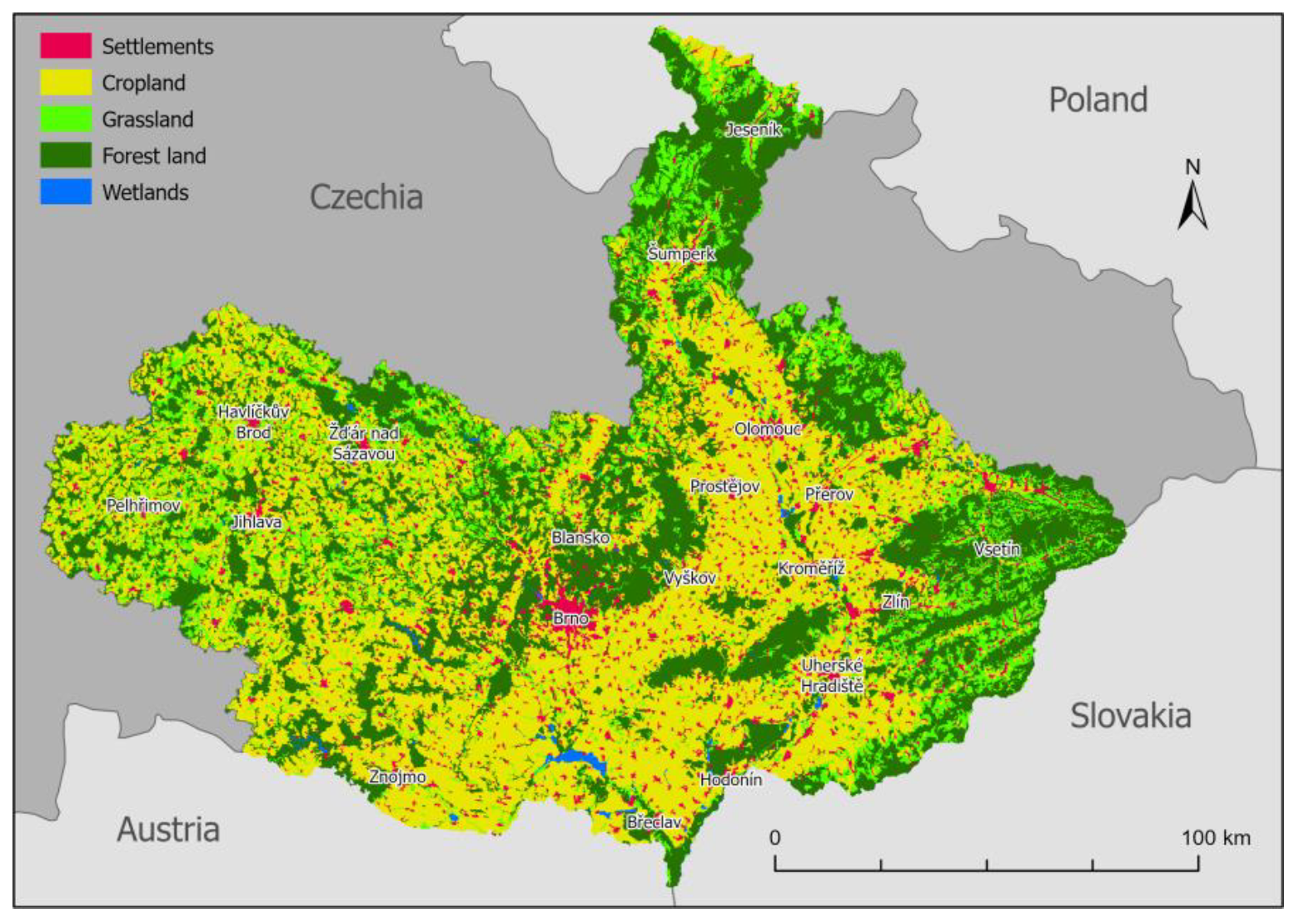
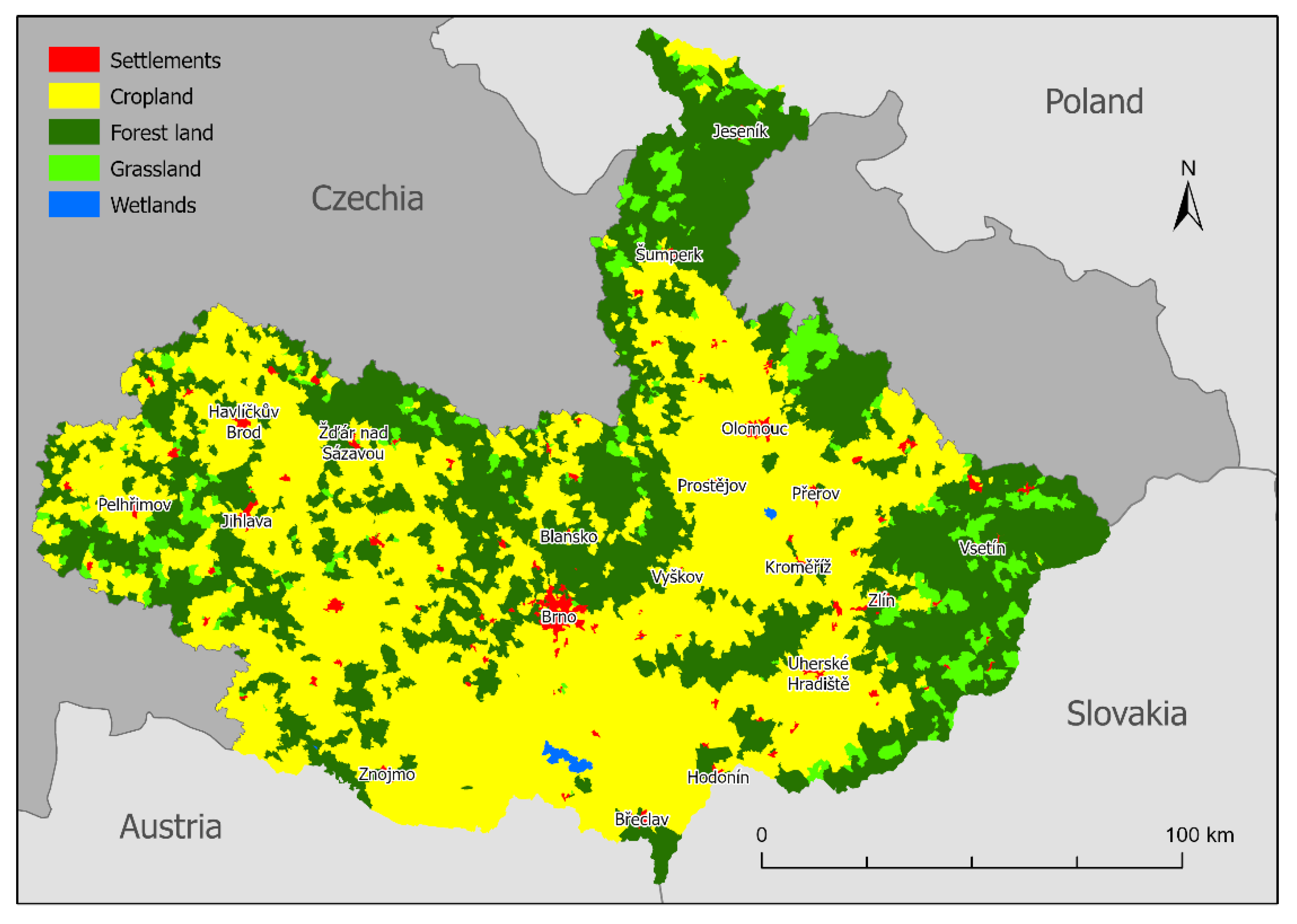
Two NUTS 2 regions were analyzed for the purposes of this study, namely, Jihovýchod (CZ06) and Střední Morava (CZ07), as shown in Figure 1. The region of interest selection was guided by the criteria of a project, “Developing supports for monitoring and reporting of GHG emissions and removals from land use, land use change and forestry”, from which this study originates (https://www.copernicus-user-uptake.eu/user-uptake/details/developing-support-for-monitoring-and-reporting-of-ghg-emissions-and-removals-from-land-use-land-use-change-and-forestry-73, accessed on 22 September 2021). The total area of the region is up to 23,217 km². The region is very heterogeneous: the lowest point is at the confluence of rivers Morava and Dyje at an elevation of 150 m a. s. l., the highest point is the mountain of Praděd, reaching 1492 m a. s. l. The longest river is Morava, which forms the axis of the region and flows from north to south. The majority of the land is used for agriculture and vineyards in the lowlands in the southern parts. From south to west, east and north, the elevation of the area gradually increases. Forests begin to dominate with increasing altitude. Deciduous forests are found at lower altitudes (at the confluence of Morava and Dyje, Chřiby and Moravský kras) and coniferous forests predominate at higher altitudes (Beskydy, Jeseníky and Vysočina), which are often formed by monocultures of Norway spruce (Picea abies). The biggest cities of the area of interest are Brno (381,346 inhabitants), Olomouc (100,663 inhabitants), Zlín (74,935 inhabitants) and Jihlava (51,216 inhabitants).

2.2. Data

Freely available Sentinel-2 multispectral images from the joint ESA/European Commission Copernicus Mission were used for compositing and classification. The images were acquired in the late spring and early summer periods of 2018 and preprocessed through the Sen2Cor algorithm [11,25]. Therefore, the atmospherically corrected data (L2A) from both Sentinel-2A and Sentinel-2B satellites were used for this research. These data are provided in 10 m spatial resolution (B2 Blue, B3 Green, B4 Red, B8 NIR bands) and 20 m spatial resolution (B5–B7 and B8A Vegetation red edge and B11-B12 SWIR bands) [11,25]. Bands with a resolution of 20 m were resampled to a higher resolution of 10 m using the nearest neighbor method. Sentinel-2 images have a 12-bit radiometric resolution but are provided in a 16-bit radiometric resolution [11], specifically through unsigned integers [19] with values ranging from 0 to 65,535. Classifications were performed in GEE using JavaScript language, where the preprocessed Sentinel-2 Multispectral Instrument Level-2A dataset is available [25,26].

The digital elevation SRTM (The Shuttle Radar Topography Mission) radar data were used for classification. The dataset is provided within the GEE platform with approximately 30 m spatial resolution as an SRTM V3 (void-filled) product. The SRTM band was used as one of the input bands for the classification process.

The Copernicus CLC (Corine Land Cover) 2018 database provided within the GEE platform and the ZM 10 map data (“Základní mapa ČR v měřítku 1:10,000”, Basic map of the Czech Republic at a scale of 1:10,000; WMS from ČÚZK) and LPIS for years 2018 (“Veřejný registr půd”, Public land register available from eAGRI; in shapefile format) were used for the creation of training and validation datasets. Historical orthophotos from 2017, 2018 and 2019 (WMS from ČÚZK) and historical imageries in Google Earth Pro software were used to verify training polygons and validation points. Google Earth Pro software provides imagery with very high spatial resolution—Maxar satellite imagery with up to 0.3 m spatial resolution (from 2015 to 2021) and CNES/Airbus with up to 0.5 m spatial resolution (from 2015 to 2021), users can examine these data using the internal Time Machine plugin.

2.3. Legend

The first basic methodological step was the creation of the classification nomenclature. The classification nomenclature follows the LULUCF regulations [15], which distinguish and report the status and development of areas of the following classes: Forest Land, Cropland, Grassland, Wetlands, Settlements and Other Land. Within the area of interest, the following classes were defined:

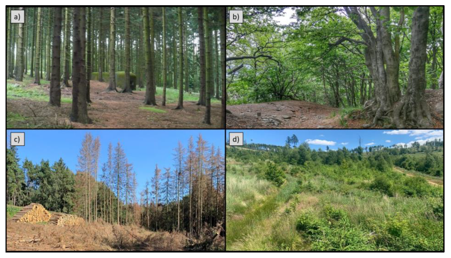
Forest Land–vegetation can be considered a forest if it covers an area of at least 0.5 ha [27] and includes woodlands and clearcut localities where there is no forest present, but is expected to grow within the next few decades.

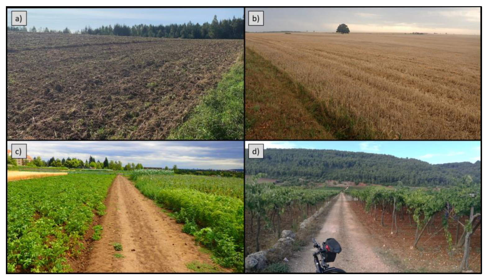
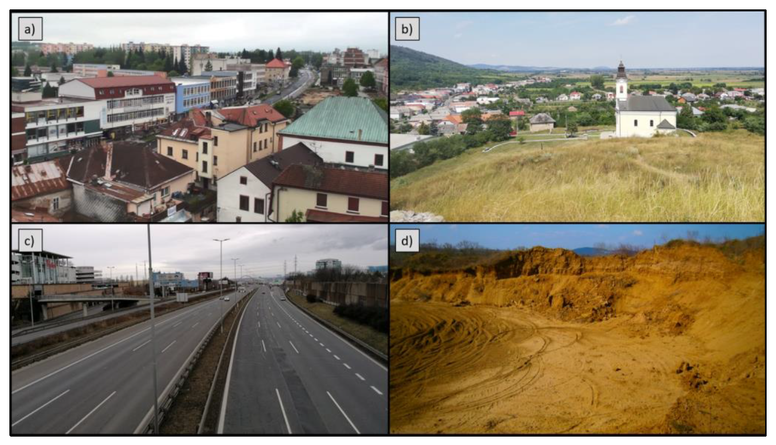
Cropland includes agricultural land and permanent crops, including vineyards, hop fields, gardens and orchards.

Grassland includes both natural and managed grasslands (pastures and meadows).

Settlements in addition to built-up areas also include roads, urban greenery, gardens near houses, landfills and active quarries.

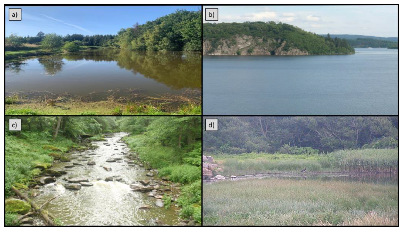
Wetlands include marshlands, bodies of water and watercourses.

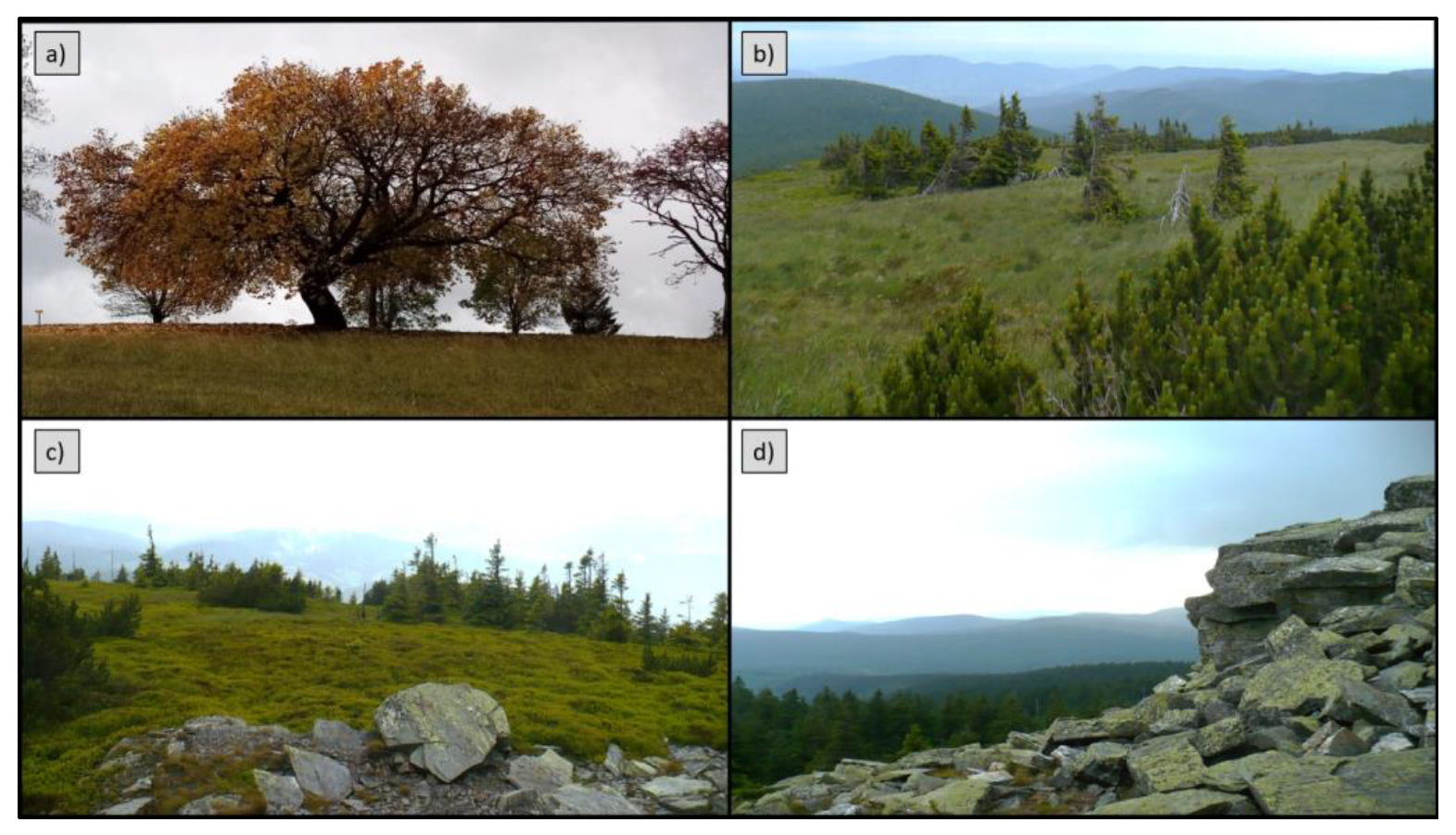
Other land mainly includes rocks, subalpine stands of dwarf Norway spruces (Picea abies) and nonnative shrub mountain pines (Pinus mugo) in the higher parts of the Czech mountains, as well as woodland/trees outside forest (ToF), such as groves and alleys, which cannot be considered as a forest according to the LULUCF regulations.

In the initial stage of classification, the Woodland class was created instead of the Forest Land class to highlight all the forested areas. Due to differences between LULUCF classes Forest Land and Other Land, the Woodland class was later divided according to the LULUCF regulations into Forest Land (polygons equal to or greater than 0.5 ha), and the remaining polygons (areas of less than 0.5 ha) were added to the results of the Other Land class during the post-classification process.

Detailed information on LULUCF classes, including their content description, is given in Appendix A.

2.4. Methods

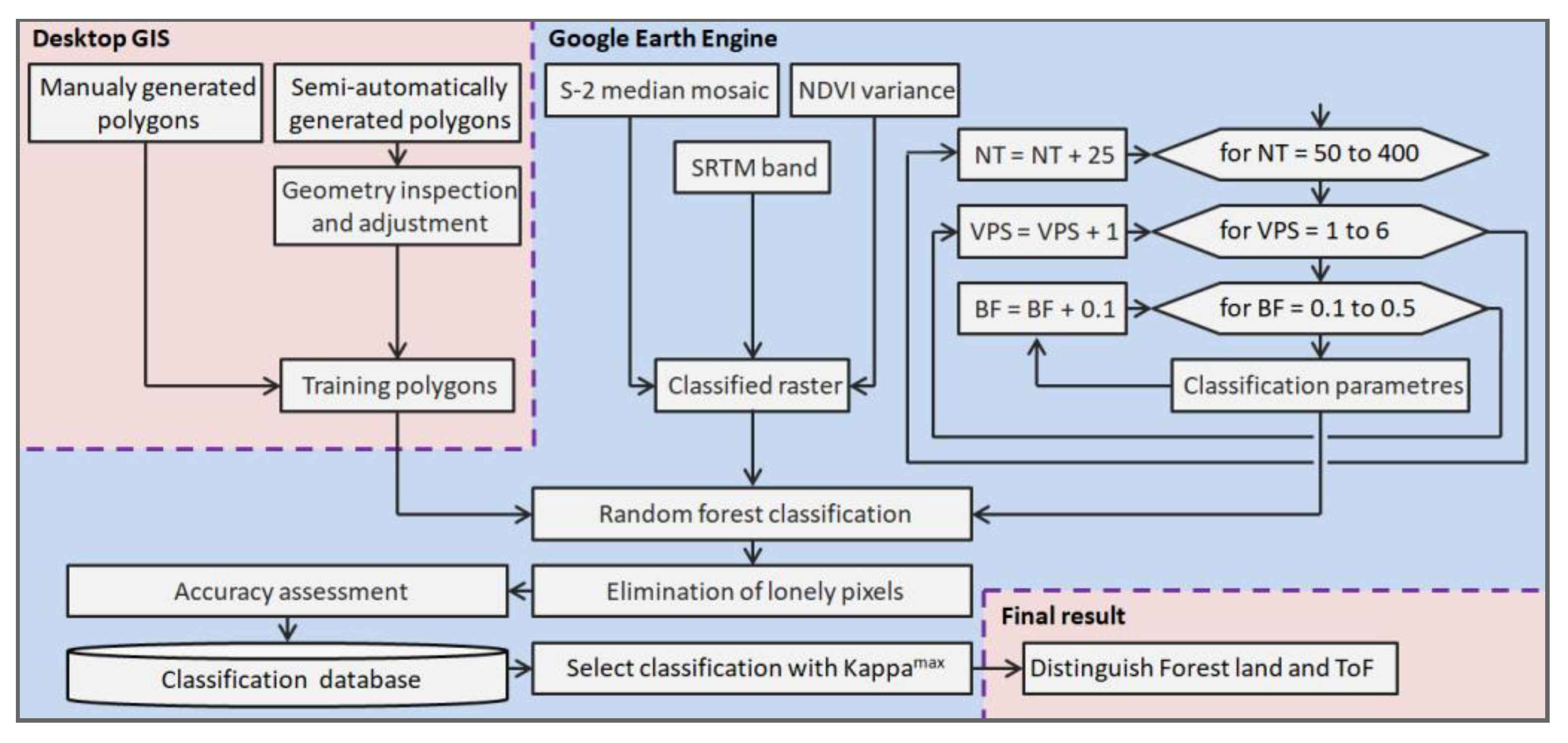
The complete methodological procedure of data processing is shown in Figure 2, which defines the procedures of preprocessing, mosaicking and classification, as well as methods for assessing accuracy and post-classification steps. The following parts describe the individual steps in more detail.

2.4.1. Cloud Masking and Mosaicking

Due to the size of the area of interest, a decision was made to create a mosaic for classification purposes. The mosaic was created by using the full potential of Sentinel-2 data, i.e., using images taken from both Sentinel-2A and Sentinel-2B. All images for mosaic creation were taken in the period from May to the end of July with a total cloud cover below 75% in the whole scene. This period was used mainly because there are only the last remnants of snow cover in the peak parts of the area of interest, and the main vegetation season takes place in the selected months. At the same time, it was the period in which there seemed to be the lowest cloud cover throughout the year 2018. This set of selected images was used in a further step—cloud masking.

For the cloud masking of Sentinel-2 data in GEE, the Sentinel-2: Cloud Probability dataset (so-called s2cloudless) was used [28]. It is constituted of a single band with 20 m spatial resolution that represents the probability of cloudiness (0–100%) for each pixel of all Sentinel-2 tiles in the entire archive. The selection of this approach was inspired by [29], who compared different Landsat 8 and Sentinel-2 cloud masking approaches, and the s2cloudless dataset significantly outperformed other methods. 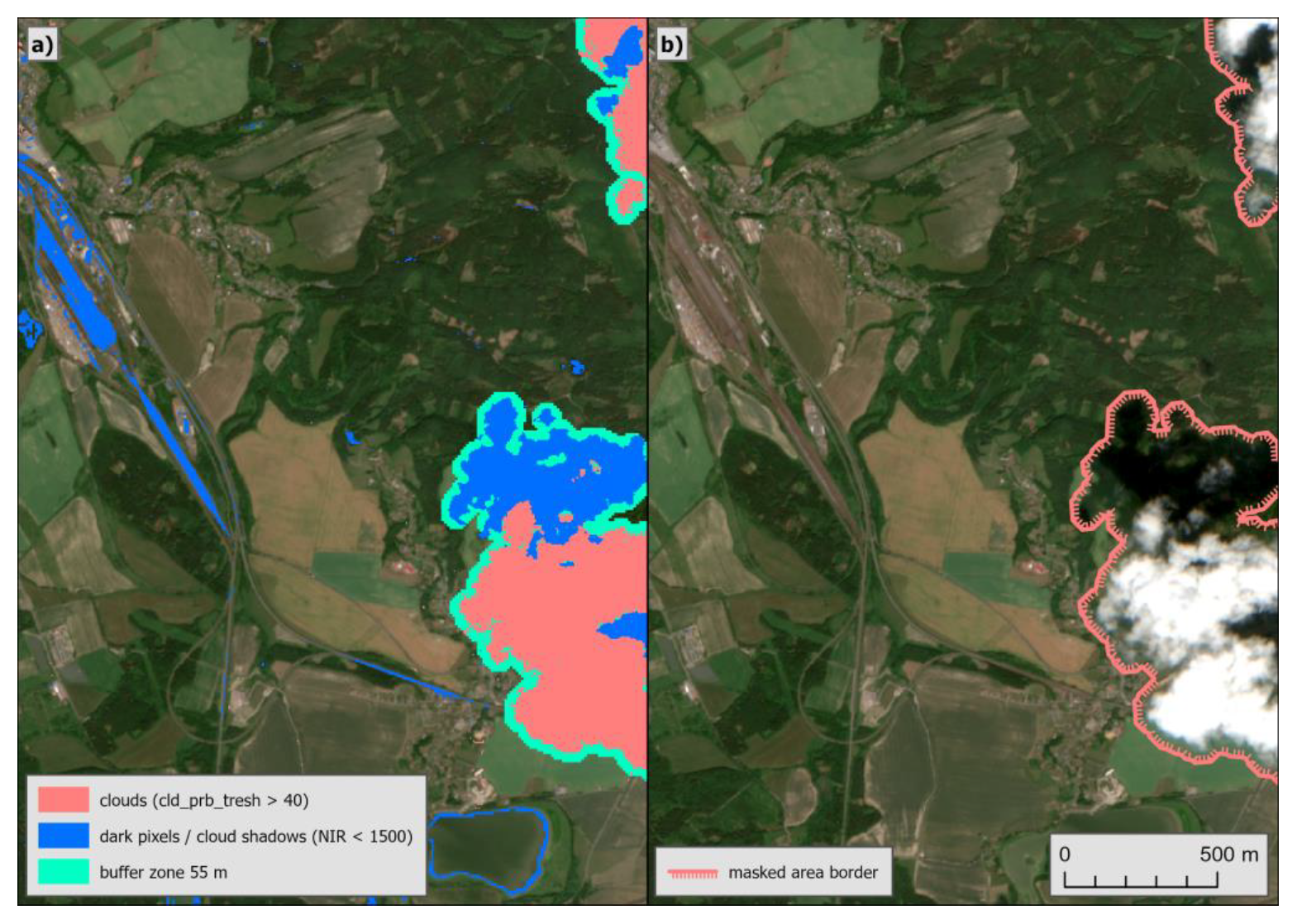Cloud shadow was detected using an algorithm developed in GEE [30], which is based on cloud projection intersection (defined by the solar azimuth angle obtained in each Sentinel-2 tile metadata) with low-reflectance near-infrared pixels. The next parameter to detect low-reflectance near-infrared pixels as the cloud shadow is a distance from the cloud. After testing and visual inspection, the following parameters were chosen for the used algorithm: cld_prb_thresh (cloud probability, where higher values were considered as clouds) = 40%, nir_drk_thresh (reflectance in the NIR band, where lower values were considered as cloud shadows) = 0.15 and cld_prj_dist (maximum allowed distance in km to search for cloud shadows from cloud edges) = 1 km; erosion 2 pixels (resolution 20 m/pixel) and dilation 5.5 pixels (buffer 3.5 pixels) were applied for the elimination of small features and gaps in clouds and shadows.

Figure 3 illustrates the process of cloud masking. Figure 3a shows the initial step of masked shadows, clouds and the created buffer. Figure 3b shows the final masked area applied to all the parameters. It is evident that not all pixels that are initially identified as clouds or cloud shadow (dark pixels) in Figure 3a were included in the final cloud mask. The final mask does not include objects that were eliminated by erosion, as well as dark pixels that are not within a defined distance and angle from the detected cloud.

At the next step, a median mosaic was created—inspired by [31,32]. All available images with lower than 75% cloud cover were selected. All S-2 bands with a resolution of 10/20 m and the NDVI index (calculated from bands B4 and B8) were used. Only pixels that were identified as cloud free were included in the median calculation. The 75% cloud cover threshold was chosen to avoid data gaps mainly in mountainous areas, where it was difficult to detect pixels not infected by clouds or cloud shadows. If high cloud cover is documented in the metadata of a scene, some areas may not be covered by clouds. This higher threshold made it possible to work with a larger number of images, which resulted in a cloud-free mosaic. The median approach was chosen because it is not as affected by outliers as the average value. 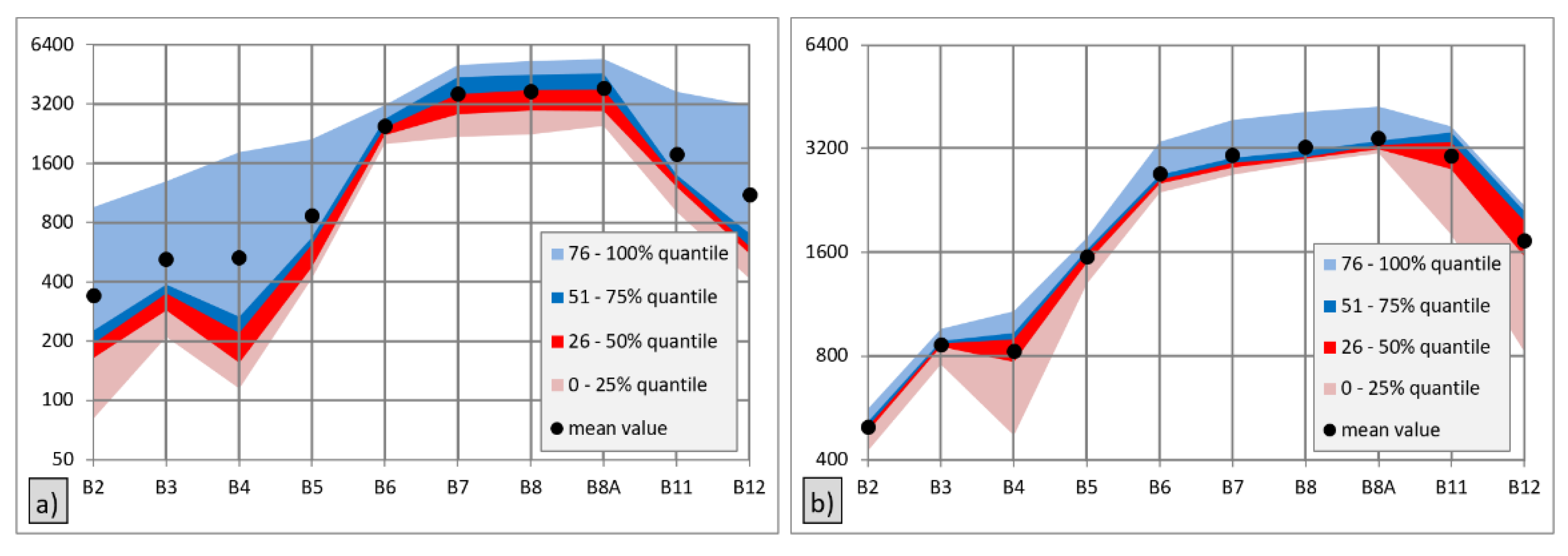Figure 4 shows a graph comparing the quantile value ranges and the average values calculated from the available unmasked values (May to July) for the selected training polygons (ID 331—Cropland; ID 488—Grassland). The mean values of surface reflectance of training polygon 331 in 6 bands of 10 were higher than 75% of the values from which these means were calculated. This was caused by outliers.

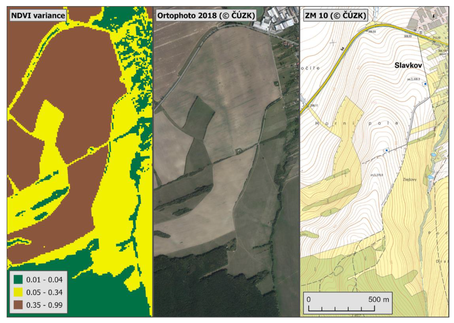
The mosaic also includes a band representing the variance of the NDVI values in the period from May to October. This band helps to distinguish relatively invariant surfaces such as buildings (small variance) from surfaces dynamically changing during the season, e.g., arable land, which refers to high variance of the NDVI value.

Figure 5 represents the variance of NDVI in the sample selected area. The map displayed on the left side of the image divides these values into three intervals. Forests and buildings have the lowest variance (see aerial image and ZM 10 in the middle and right map fields), and grasslands have a higher variance (visualized in yellow on ZM 10). Arable land shows the highest NDVI variance.

Another band added to the resulting mosaic was SRTM DEM containing altitude data with a spatial resolution of 30 m. The SRTM band was used together with Landsat 8 multispectral satellite data in [31]. These data were important for distinguishing similar surfaces in terms of land cover, but different land use approaches for LULUCF purposes. Examples are stone and paved surfaces, where it is necessary to distinguish blockfields (Other Land) from paved areas within the Settlements class. The resulting mosaic has a spatial resolution of 10 m. All input data with a resolution lower than 10 m (S-2 bands with a resolution of 20 m and SRTM with a resolution of 30 m) were resampled using the Nearest Neighbor method.

The significance of the bands for classification was recorded using Gini importance for the 4 parameter combinations in Appendix C. As can be seen in Appendix C, the importance of SRTM elevation and NDVI variance is the most significant, whereas the B8 band is of the least importance.

2.4.2. LULUCF Classification

The Random Forest (RF) method was selected, tested and used for classification. This method has been successfully used in the classification of multitemporal satellite data, e.g., [18,31]. Compared to other classification algorithms (CART, SVM, kNN and MLC), this method achieved the best results in many studies [17,32,33,34]. It is a method of controlled nonparametric classification using machine learning. Its essence is the creation of decision trees, where each tree individually evaluates to which class each individual pixel belongs; see [16,34]. The basic parameter is the Number of Trees (NT). Other adjustable classification parameters are the Variables per Split (VPS), Bag Fraction (BF), Max Nodes and Min Leaf Population.

2.4.3. Training Polygons

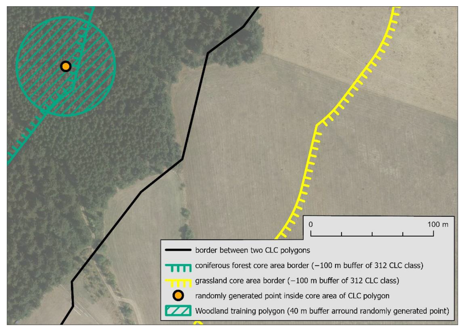
An important aspect of the resulting classification accuracy is the training data. The training polygons for this study were created by two methods. The first method is the semi-automatic creation of training polygons within the CORINE Land Cover 2018 (CLC 2018) vector layer. The second method was the manual creation of the additional training polygons.

From the CLC 2018 polygon database, the core areas of the training polygons were created using the Buffer function with the following parameter: −100 m. Inside these areas, training polygons of a circle shape with a diameter of 80 m were randomly generated. This can be seen in Figure 6, where one of these training polygons is visualized. These polygons/circles were generated with 2500 m minimal distance.

For some evaluated classes/surfaces, no training polygons were used in the procedure above. It is given by both geometric and thematic characters. For example, in the case of watercourses, this is due to the fact that no polygon in this class has a core area of 100 m inwards. Only one polygon was generated for the other land class, which, however, did not include some important elements of this class, e.g., no training polygon was created on the territory of a photovoltaic power plant. Therefore, 7 training polygons were manually created for the Other Land class, 5 of them were located in rubble fields in the Hrubý Jeseník mountains; in one case, they were rocks in the Suché skály nature reserve, and in another case, they were scrub mountain pines in the alpine vegetation zone of Hrubý Jeseník. Polygons for specific areas of mountain meadows in the Beskydy mountains were collected manually. Training polygons for peatbogs and reeds were added to the Wetlands category. Due to the high heterogeneity of the Cropland class, some polygons were added to cover some specific types of land cover. It was found during preliminary classification testing that some areas within the Cropland class were misclassified as other classes. As a result, some additional training polygons were manually added at these localities. 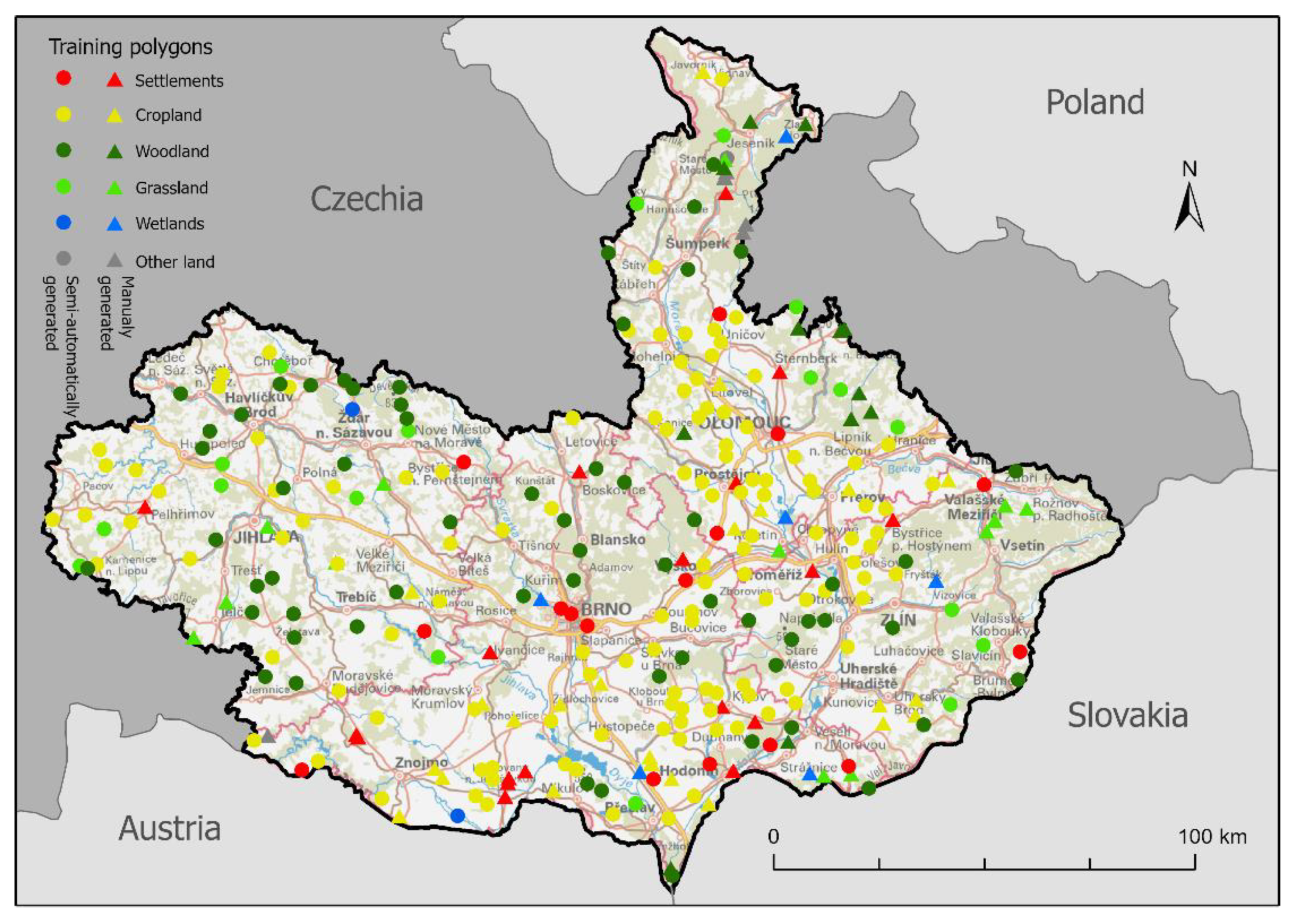Polygons that were deforested due to droughts and bark-beetle disturbances (Ips typographus) and are currently in the initial stages of forest growth were also created. Cropland and Grassland polygons were also manually added to better differentiate these surfaces. A total of 299 training polygons were created; their distribution within the area of interest can be seen in Figure 7. The number and structure of manually added training polygons are shown in

Table 1. Amount of training polygons for individual training classes.

Class LULUCF	Semi-Automatically Created Polygons	Manually Created Polygons	Total
Settlements	16	18	34
Cropland	122	24	146
Woodland	60	12	72
Grassland	18	13	31
Wetlands	2	6	8
Other land	1	7	8
Total sum	219	80	299

.

A conversion table of CLC to LULUCF classes was created to systematically determine the LULUCF class. The individual training polygons determined from CLC belong to the LULUCF class, which was decided based on this conversion table, as presented in Appendix B.

All created training polygons from the CLC were verified using an orthophoto to check if their declared land cover matched the LULUCF class. This verification was performed using orthophotos from ČÚZK available for the area of interest. Most of the images of the area were captured in 2018, and only the western parts of the area were missing images from the same year; therefore, images from 2017 and 2019 were used. If the land cover of the checked training polygon did not change in aerial photographs in this time interval (2017–2019), there was no reason to consider the class incorrectly assigned. If the specified orthophoto land cover did not match the declared CLC land cover, the training polygon was deleted or manually adjusted to be within the declared land cover. Therefore, emphasis was placed on the polygon lying in its entirety in one class without interfering with other classes. The affiliation of training polygons to the Grassland class was checked using LPIS data and ZM 10 maps from ČÚZK. This detailed inspection was carried out due to the difficult to distinguish Cropland and Grassland classes using orthophotos.

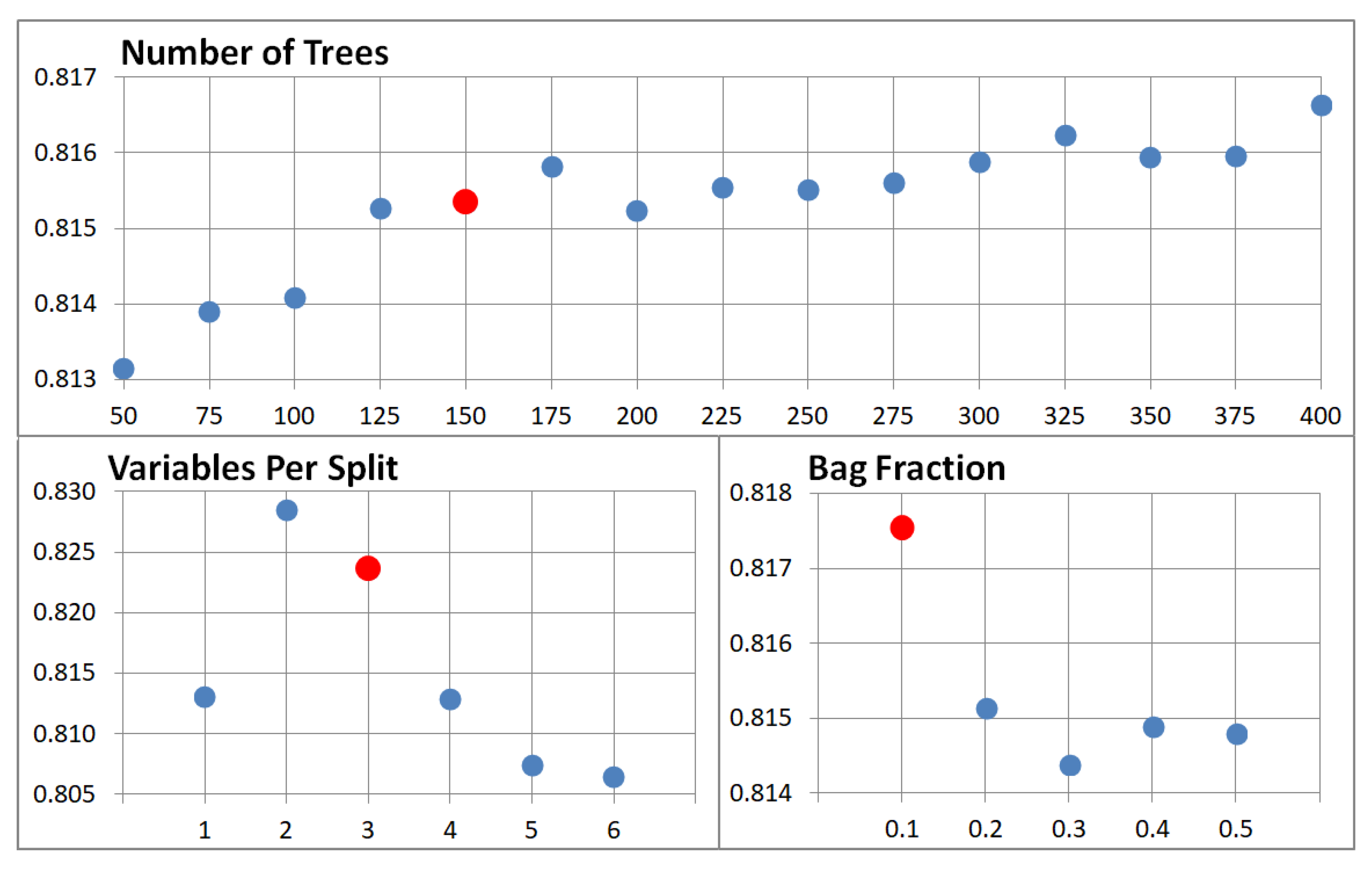
2.4.4. Parameters of Classification

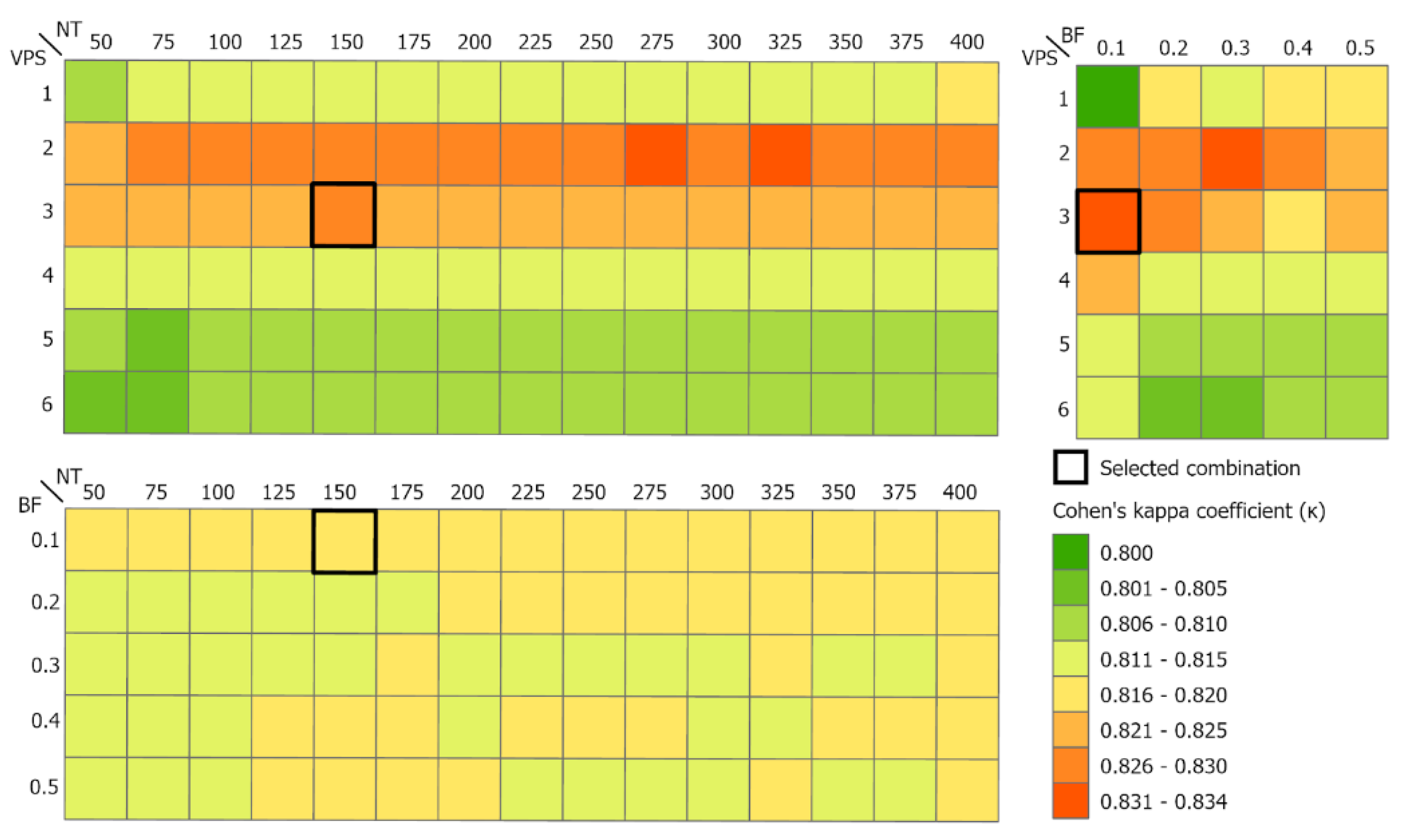
In the classification process, the most important task was to define a combination of parameter settings that would deliver the highest accuracy. The Number of Trees parameter was tested from 50 to 400 at 25-tree intervals, the Variable per Split parameter was tested from 1 to 6 at 1-variable interval and the Bag Fraction parameter was tested from 0.1 to 0.5 at 0.1-fraction intervals. The other Max Nodes parameters were left with the default value ‘NULL’, that is, without limits, as well as the default value of 1 for the min Leaf Population. A total of 450 combinations of the parameters Number of Trees, Variables per Split and Bag Fraction were generated and evaluated.

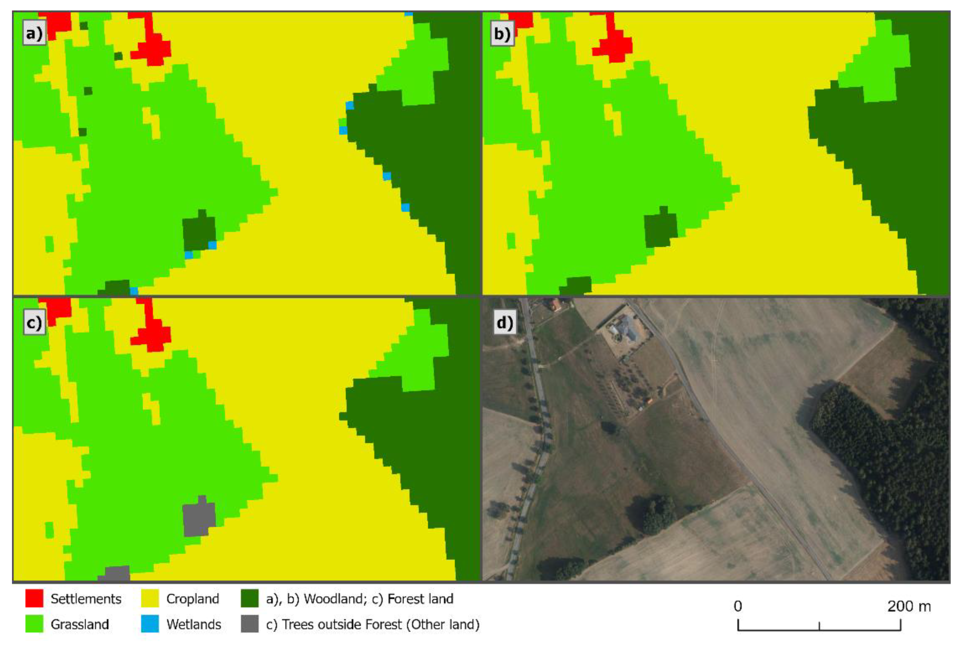
Per-pixel classification often brings a ‘salt-and-pepper’ effect. This effect was eliminated by filtering and replacing isolated pixels with neighboring values. At this step, the areas represented by one pixel were eliminated and replaced by the majority value of the pixels in the 3 × 3 kernel window filtering. The point of this step is documented in Figure 8a,b. The main complication is the pixels on the borders between two classes, or in the case of tree growth, trees can cast shadows into their immediate surroundings, which are mostly incorrectly classified as Wetlands. These lonely pixels were filtered. The minimum mapping unit of the classification is 2 pixels, i.e., 200 m².

2.4.5. Accuracy Assessment

The validation points were created in the ESRI ArcGIS Pro software, where the Create Accuracy Assessment Points tool (Spatial Analyst) was used. A total of 2235 points were created (in WGS 84/UTM zone 33N EPSG: 32633 coordinate system), and the Stratified Sampling method based on preliminary classification testing was used for the accuracy assessment and random creation of control points [24]. The affiliation of control points to the LULUCF class was performed in the same way as in the case of training polygons; see Section 2.4.3. Due to the low number of control points generated randomly for the Other Land, 31 points in this category were manually created. For effective validation, an innovative algorithm was created in the cloud-based platform GEE. The control points were uploaded to GEE, where the Classifier package was used to validate the classifications. Specifically, the classifier.confusionMatrix() function was used for confusion matrices and the errorMatrix() function for overall accuracy [35] and the ConfusionMatrix.kappa() function for the Kappa index by [36]. The Kappa index value (Cohen’s Kappa) was calculated for each combination of input parameters. The combinations of input parameters that achieved the highest Kappa index value were selected, and validation matrices and overall accuracy were subsequently generated for them. The combinations of parameters with the highest accuracy were selected as the most suitable for classification.

2.4.6. Post-Processing Classification

According to the definitions of LULUCF, tree growth with an area of less than 0.5 ha cannot be considered as a forest, but as trees outside forest (ToF). For this reason, all Woodland growths with an area of less than 5000 m² (less than 50 pixels) were converted to the Other Land class. Figure 8b the state before the division of the Woodland class into Forest Land and ToF and in Figure 8c the state after the division. Based on this step, the minimum mapping unit for Forest Land differed from the other categories and was 5000 m² (0.5 ha).

3. Results

3.1. Influence of Parameter Selection on the Resulting Accuracy of Classification

One of the main goals of the study was to develop an RF-based classification method that allows the classification of Sentinel-2 data in GEE according to the LULUCF requirements. In terms of classification, the most important task was to find the most suitable combination of RF classifier input parameters that will lead to the highest accuracy of the LULUCF classification. The evaluated parameters were Number of Trees, Variables per Split and Max Nodes. For this purpose, an innovative script was developed in the GEE environment, which can evaluate hundreds of combinations of input parameters in a short time and use the overall accuracy and Kappa index to select the combination with the highest accuracy achieved.

From the achieved results of individual combinations (Appendix E), it was seen that the highest value of the Kappa index (κ) was achieved in the case of a combination of the settings of the parameters NT: 150, VPS: 3 and BF: 0.1 with the value κ = 0.8383. At the same time, this setting of the examined parameters achieved the highest overall accuracy of all combinations, with a value of 89.01%. The results of κ and the overall accuracy for the individual parameter combinations are given in Appendix E.

Upon closer inspection of the settings and relevance of individual parameters, the average values of κ (calculated from testing control points) for individual values of input parameters are documented in Figure 9. In the case of the NT parameter, each average value was calculated from a total of 30 κ values (6 combinations of the VPS parameter and 5 combinations of the Bag Fraction parameter), the Variables per Split parameter was calculated from 75 values and the Bag Fraction was evaluated from 90 κ values. The parameters values used for the final (most accurate) classification are highlighted in red. If we look at the values obtained from individual parameters, then the average value κ of the NT parameter had an ascending character, together with the number of trees, and the highest value of κ was reached at the maximum number of trees (400). However, the increase in the value of κ from 150 was no longer as significant. The value of 150 trees was evaluated as the most suitable in combination with other parameters. For the VPS parameters, the highest average value of κ was reached at the parameter value of 2. A comparatively lower average value was obtained by the value of parameter 3, which was selected for the combination of the final classification. This parameter also had the largest range of the minimum and maximum average values of κ, which may indicate that this parameter has a significant effect on the resulting combination for the most accurate classification. For the Bag Fraction parameter, the highest average value of κ matched the finally selected value of 0.1. Other BF parameter settings evaluated had lower κ values.

Figure 10 describes in detail the average values of κ for the pair of evaluated parameters. The average values of the combination of VPS and NT (VPS/NT) were calculated from 5 values of κ, the combinations of BF and NT (BF/NT) were calculated from 6 values of κ and the combinations of VPS and BF (VPS/BF) were calculated from 15 values.

When evaluating a VPS/NT combination, the VPS parameter values are expressed in rows and NT in columns. The highest values of κ were reached by the combination NT = 275 and VPS = 2 (NT = 150, VPS = 2 are the values used in the final combination of three parameters for classification). The values of κ did not change much in the rows, unlike the evaluated NT parameters in the columns. Therefore, the average value of κ is more affected by the VPS parameter than the number of trees (especially obvious when setting the number of trees above 50). The high relevance of the VPS parameter is also evidenced by the evaluation of the VPS/BF parameter combination; in this case, the VPS influence appears even stronger. The combination with the highest value of κ (BF = 1, VPS = 3) was the same, which was selected as the most suitable in the combination of all three parameters. When comparing these two parameters, the largest difference between the maximum and minimum average values of κ was evident. On the contrary, the smallest differences in the variability of κ values could be seen by comparing combinations of BF/NT parameters. The values of κ were found in the relatively narrow range of 0.811–0.820. BF = 0.1 and NT = 150 are the values contained in the resulting combination of three parameters.

3.2. Accuracy Assessment of the Classification

In addition to the calculation of κ, the values of overall accuracy (OA) and validation matrices were calculated for a detailed evaluation of the accuracy of the classification. The validation matrix for the resulting combination of classification parameters (NT: 150, VPS: 3 and BF: 0.1) is documented in

Table 2. Validation matrix of the final classification.

	Settlements	Cropland	Woodland	Grassland	Wetlands	Other Land	User Accuracy
Settlements	107	26	10	18	1	0	66.05%
Cropland	8	882	6	26	1	0	95.56%
Woodland	1	11	728	32	0	0	94.30%
Grassland	1	54	23	243	1	0	75.47%
Wetlands	0	5	1	1	17	0	70.83%
Other Land	16	1	0	1	0	14	43.75%
Producer Accuracy	80.45%	90.09%	94.79%	75.70%	85.00%	100.00%	Overall accuracy 89.01%

. The overall accuracy reached 89.01%, and Cohen’s Kappa was 0.8383 for this combination. When a closer inspection of the producer accuracy and user accuracy values was performed, Settlements were most often misclassified as the Cropland class. On the contrary, the Other Land class was most often misclassified as Settlements. More validation points of Settlements were classified as another class than validation points of other classes classified as Settlements. It follows that the Settlements class should have a slightly undervalued classified area. Cropland was most often misclassified as Grassland and, conversely, Grassland was most often misclassified as Cropland. Changing the Grassland class to the Cropland class with an amount of 54 points was the most common change in the classification and accounted for about one-fifth of all errors (2.24% of all validation points). The Cropland class appeared to be slightly overvalued (especially at the expense of Grassland). The Woodland class was most often misclassified as Grassland and vice versa. This could be caused by grass-like clearings that formed in the forests after the trees were logged. This type of forest could be observed within the area of interest due to bark beetle calamities and droughts consequences. The Wetlands control points were most often misclassified as the Cropland class. The main cause of this phenomenon could be seen in the location of control points in places where there are swamps, reeds and peat bogs, i.e., wetlands with a more substantial representation of the vegetation component. When comparing user accuracy and producer accuracy, the Wetlands class appeared to be slightly underestimated. The Other Land class seemed to be clearly underestimated, as less than half of the points belonging to this class were correctly classified (confusion mainly with Settlements). On the other hand, no control point from any other class was classified as Other Land.

The LULUCF classification was performed in the area of interest with a heterogeneous character both from a physical–geographical and socio-economic point of view. The heterogeneous character of the area was determined by the diverse representation of individual LULUCF classes. From the results documented in

Table 3. Areas and representations of individual LULUCF classes according to the final classification.

Class	Area	Percentage
Settlements	1059.8 km2	4.56%
Cropland	9936.4 km2	42.80%
Forest Land	8259.6 km2	35.58%
Grassland	3560.7 km2	15.34%
Wetlands	178.6 km2	0.77%
Other Land	222.1 km2	0.96%

and Figure 11, it is clear that the Cropland class had the highest area in 2018 with more than 42% of the total area. Grassland class occupied over 15%. The total area of agricultural land, i.e., Cropland and Grassland, accounted for 58%. Around 36% of the area of interest was classified as Forest Land, which is close to the average forest area in the Czech Republic (34%). The Settlements area was close to 5%. The remaining two categories did not exceed 1%, the Wetlands class occupied 0.77% and the Other Land occupied 0.96% of the area.

Figure 10 shows the spatial distribution of the classes examined. Large areas of the Cropland class occur in the most fertile areas south of Brno and in the vicinity of Olomouc. Forest growth occurs mainly in less fertile mountain regions on the eastern and northern edges of the area of interest, also in highland areas around Brno (Drahanská vrchovina and Chřiby). The Grassland class dominates in less favored areas for agriculture (LFA) in mountain and foothill areas, especially in the Beskydy, Hrubý Jeseník and Nízký Jeseník. The heterogeneous composition of the land cover can be seen in the hills in the western part called Vysočina (around the towns of Jihlava, Pelhřimov, Havlíčkův Brod and Žďár nad Sázavou). It is the most heterogeneous area within the area of interest. Significant water surfaces are located around Novomlýnské reservoirs and near Tovačov, where there are large anthropogenic lakes created after sand mining.

In addition to the LULUCF class map for the entire evaluated area, scale-detailed maps of 3 selected areas are provided in Appendix D. The first area documents LULUCF between the Pilská reservoir and the village of Polnička. The local landscape is a composite of individual monitored classes. To the south of the village Polnička there is a quarry, which was successfully classified as Settlements according to the LULUCF nomenclature. In the middle row, the documented area has been strongly anthropogenically affected. There is a D1 highway with widely developed road infrastructure and large construction complexes. Both surfaces were well classified as Settlements. The sparsely built-up areas of the villages of Pávov and Nový Pávov (in the west) were also well classified. The bottom row shows the area inside the Libavá military district, which has been severely affected by droughts and bark beetle disturbances. In the case of this area, certain weaknesses of the classification algorithm were documented, where some pixels without vegetation were incorrectly classified as Settlements. On the other hand, most of the affected forest area was successfully classified as Forest Land.

4. Discussion

The main aim of this study was to develop an RF-based classification method that allows the classification of Sentinel-2 data according to LULUCF requirements. Multispectral satellite data from the Sentinel-2 mission were used for their advanced spatial and temporal resolution. Methodological procedures were developed and implemented in the freely accessible cloud platform GEE. The methodology was tested, and the results were validated for a larger region (two NUTS 2 units with a total area of 23,217 km²) in Czechia using data collected in 2018. A motivation of this study was to prove a high relevance and perspective of EO data from the Copernicus program for LULUCF reporting. LULUCF reporting in Czechia has been exclusively based on cadastral land use information, which has several weaknesses that affect the quality of the collected data [22,23]. The compatibility of the cadaster land use with defined LULUCF classes is also problematic. For example, the Other Land class in the cadastral register includes highly diverse surfaces that should be divided into individual LULUCF classes.

From the research point of view, the most important task was to test the Random Forest classifier for the purpose of LULUCF classification. Although LULUCF classes often include very different surfaces in terms of spectral reflectance, the positive finding is that the use of an RF classifier did not require these surfaces to be classified as separate classes and subsequently aggregated. Thus, quite different surfaces within one LULUCF class entered the classification, such as orchards and arable land as the Cropland class, or built-up areas and roads as the Settlements class. The Random Forest classifier was able to correctly classify these surfaces with relatively high accuracy. However, the basic condition was the quality of training. A semi-automatic method was developed for the creation of training polygons using the CLC 2018 database to provide high-quality training of the monitored classes. However, for minority classes and specific surfaces (approximately less than 2% of the total area), this method was not able to fully ensure a sufficient number of training polygons. For such classes, it was necessary to create training polygons manually.

A relevant research aspect was to test and find the most suitable combination of Random Forest classifier input parameters (Number of Trees, Variables per Split and Bag Fraction) to achieve the highest classification accuracy. For this purpose, an algorithm was created in GEE, which allows a large number of combinations of input parameters to be tested and then the one that achieves the highest accuracy to be selected. From the achieved results of individual combinations accuracy, the highest value of the Kappa index and the overall accuracy were achieved in the case of the use of the following combination of parameters NT: 150, VPS: 3 and BF: 0.1 with the value κ: 0.8383 and the overall accuracy of 89.01%. Comparing the obtained results, where GEE was used for RF classifier implementation, in [31,37,38], the number of trees 100 and other parameter values were used as the default in GEE (VPS is default defined as the square root of the number of bands of an image; BF is 0.5). Such a setting would lead to the result κ: 0.8206 and OA: 87.87% in this study. The RF classifier was also used to map Cropland in Southeast Asia using GEE [39], where the method defined a value of 300 as the most appropriate NT and left the default value for other attributes. If this setting was used in this work, the result would be κ: 0.82 and OA: 87.79%.

The LULUCF classification used in this study is based on a multitemporal approach that uses several images during the observed vegetation season. Due to the large extent of the area of interest and multitemporal approach, it was decided to create a mosaic for classification purposes. The mosaic was created using the full potential of Sentinel-2 data; all images taken in the period from May to the end of July with a total cloud cover below 75% were used to create the mosaic. The Sentinel-2: Cloud Probability dataset (so-called s2cloudless) was used for the cloud masking of Sentinel-2 data in GEE [29]). However, according to the results of experiments within this study, masking clouds shadows remain a complicated and poorly elaborated task in the s2cloudless dataset. For this reason, another algorithm in GEE was used [30]. Shadows are defined by cloud projection intersection with low-reflectance near-infrared (NIR) pixels. The median method was chosen to create the resulting mosaic. For each pixel, a median of the cloudless values was determined as the final value. This method was proven to be suitable for such a large area with very heterogeneous conditions prevalent throughout the year. In the case of the median, it is advantageous to eliminate the influence of the resulting mosaic by outliers caused by noise or due to imperfections of cloud correction. This method allows the elimination of time-limited/exceptional surface conditions. For example, rapeseed (Brassica napus) has a highly different reflectance during the full flowering period compared to before or after flowering. This flowering phenological phase negatively influences the classification of the broadly defined LULUCF class Cropland. The choice of suitable tiling methods was also tested by [32], who evaluated the effect of using the tiling method on the resulting overall accuracy value. The mosaic created by averaging the available surface reflectance values was classified by 88% accuracy and the median mosaic had an accuracy of less than 86%. However, it should be noted that it dealt with the classification of three less large areas (25 km²) in Calabria (southern Italy) with lower heterogeneity and minimal cloud cover in the summer months. Another study [38] created a classified mosaic for each Landsat 8 and 7 spectral band as the 75th percentile of six values representing the average reflectance over each of six two-month periods (January–February, March–April, …) during a year. In [40], a classified mosaic was created using a minimum value for each month to ensure that the resulting values were not affected by clouds. This approach does not seem to be the best solution after the experiences in this study, because the recorded minimum values were often hit by a cloud shadow.

In addition to the selection of the specific mosaicking method, the decision on the length of the time interval from which images will be used remains an important research question. In this work, the interval of 3 months from May to the end of July was used. Based on the testing, this interval was chosen because it was a period that covers significant vegetation/phenological phases and from which it was possible to create a mosaic based on relevant values for the entire area of interest. The selection of time period is also dependent on weather conditions, especially cloudiness, which could be various for different years. For this reason, it is not possible to recommend a standard optimal time period. The 3-month median mosaic was also used in [41] to map cropland using the Random Forest in China. The mosaic was created together with images from Landsat 8 and 7. In [39], cropland in Southeast Asia was analyzed using a time interval of 4 months for the mosaic.

The input of altitude values from DEM (SRTM) in the classification proved to be highly useful. According to the calculated Gini importance, it was the most important band in the classification (Appendix C). This band also reached the highest significance in the case of the study [31], which classified the territory of Mongolia using Landsat 8 and SRTM data. Another significant input was the calculated NDVI variance band for the period from May to October. The choice of this input information was inspired by several previous works, e.g., in [38], arable land mapping (corresponding to the Cropland class) was performed using Random Forest. When classifying, he used the standard deviation of NDVI from the observed three years. In terms of Gini importance determination, the standard deviation of NDVI achieved the fifth highest relevance from the twelve compared. The elevation, slope, range of NDVI and minimum of NDVI had higher relevancy in [38]. In the case of this work, the NDVI variance band was second in terms of importance.

From the point of view of the data used, the Sentinel-2 data appear to be a promising data source for LULUCF purposes. This is evidenced by several studies that have successfully used Sentinel-2 data to classify similar LULUCF classes [12]. This study confirmed the high relevance of modern classification methods based on machine learning (specifically RF) and the high perspective in the use of cloud-based technologies. The GEE environment is undergoing dynamic development due to its free availability for noncommercial use and its wide range of data and useful algorithms.

Considering the shortcomings of the data and methods used in this work with regard to the LULUCF regulations, an important aspect is the use of satellite data, which reflect land cover classification rather than information on land use. However, the LULUCF methodology is based more on a land use approach. From this point of view, the following research steps should focus on the possibilities of combining satellite data (Sentinel-2, Planet.com) and cadastral data with the maximum use of the advantages of these data sources for the purposes of accurate and time-compatible reporting. The LULUCF classification method, which would be based on standardized data (Copernicus data), could deliver comparable (harmonized) LULUCF results for use in the IPCC and could be applicable in many countries around the world. To evaluate the accuracy and applicability of the proposed method, it is necessary in the future to focus on the evaluation of LULUCF changes over several years. Classification inaccuracies may be more noticeable in change detection between two time periods. Moreover, it would be useful to use alternative methods for accuracy assessment, e.g., Mapcurves GOF for categorical variables. The created algorithm is placed and open in Github to be freely used and developed: https://github.com/hawk919/LULUCF-GEE-classification/blob/main/CODE.

5. Conclusions

LULUCF is a greenhouse gas inventory sector that reports the extent of and changes in the following classes: Settlements, Cropland, Forest Land, Wetlands and Other Land. Due to the international scope, different methodologies with different data are used. LULUCF data from Czechia are reported based on cadastral data, which have limited abilities to detect land-use changes [22,23]. On the other hand, EO data and methods have been significantly developed in recent periods, especially due to important programs and missions, i.e., Copernicus or Landsat. For this reason, the main aim of this study was to use and test the Sentinel-2 data for the purpose of LULUCF in the two selected NUTS 2 regions in Czechia in 2018. The methodological workflow was implemented in the freely accessible platform GEE. From the research point of view, the most important task was to find the most suitable combination of Random Forest classifier input parameters (Number of Trees, Variables per Split and Bag Fraction) to achieve the highest classification accuracy. The classification with the highest accuracy (the overall accuracy of 89.1% and Cohen’s Kappa of 0.84) was achieved with the following combination of parameters: NT = 150, VPS = 3 and BF = 0.1. It was proven that the parameter VPS was of the greatest importance for the accuracy of the classification. To select and evaluate the relevance of parameters, an innovative algorithm was developed in GEE, which enabled the simultaneous execution and evaluation of 450 classifications at once. This innovation is probably the biggest benefit of this work, because this method allows the users to operatively evaluate and select suitable classification parameters for the area of interest in a short time.

Due to the large extent of the area of interest and multitemporal (multiple images) approach, it was decided to create a mosaic for classification purposes. The mosaic was created to exploit the full potential of Sentinel-2 data. For this reason, all images taken in the period from May to the end of July with cloud cover lower than 75% were used. The median method was chosen to create the resulting mosaic. This method was proven to be suitable for such a large area with very heterogeneous conditions prevalent during the year. Moreover, altitude values derived from SRTM and NDVI were added in the mosaic and used in the classification. The input of altitude values was highly useful, and according to the calculated Gini importance, it was the most important band in the classification (similar to the study [31]). The NDVI variance values were the second most significant in terms of Gini importance.

Another goal was to create a LULUCF classification nomenclature for Czechia with a detailed semantic description and maximum compatibility with LULUCF. To ensure compatibility with the LULUCF approach, the Woodland class was originally created and subsequently divided into Forest Land (areas greater than 0.5 ha) and Other Land (trees outside the forest area of less than 0.5 ha). The results of the classification show that the most dominant LULUCF classes within the area of interest in 2018 were Cropland and Woodland/Forest Land. The highest classification accuracy of over 90% was achieved for the classes Cropland and Woodland. In terms of user accuracy, the Settlements (66.05%) and the Other Land (43.75%) were the most problematic classes.

The developed method is based on the classification of Sentinel-2 data using the Random Forest classifier in the cloud-based platform GEE. This approach seems to be very promising for the systematic implementation of EO data in LULUCF. The Sentinel-2 data from Copernicus programme appear to be a relevant data source for LULUCF purposes. The following research steps should focus on the possibilities of combining satellite data (Sentinel-2) and cadastral data with the maximum exploitation of the advantages of individual data sources for the purposes of time-compatible LULUCF reporting. For this reason, it is necessary to focus on the evaluation and validation of LULUCF within a longer period and assess the accuracy of the changes. The cloud-based classification method, which would be using the standardized data (Copernicus data) and would be applicable in many countries around the world, could bring significant progress in the use of EO data in LULUCF. A closer dialogue between stakeholders/end-users and EO experts is the next important step for that goal.